Optimal Time–Jerk Trajectory Planning for Manipulators Based on a Constrained Multi-Objective Dream Optimization Algorithm

Abstract

A multi-objective optimal trajectory planning method is proposed for manipulators in this paper to enhance motion efficiency and to reduce component wear while ensuring motion smoothness. The trajectory is initially interpolated in the joint space by using quintic non-uniform B-splines with virtual points, achieving the C⁴ continuity of joint motion and satisfying dynamic, kinematic, geometric, synchronization, and boundary constraints. The interpolation reformulates the trajectory planning problem into an optimization problem, where the time intervals between desired adjacent waypoints serve as variables. Travelling time and the integral of the squared jerk along the entire trajectories comprise the multi-objective functions. A constrained multi-objective dream optimization algorithm is designed to solve the time–jerk optimal trajectory planning problem and generate Pareto solutions for optimized trajectories. Simulations conducted on 6-DOF manipulators validate the effectiveness and superiority of the proposed method in comparison with existing typical trajectory planning methods.

1. Introduction

Offline multi-point smooth trajectory planning is a critical core technology in robotics, directly determining the operational efficiency and task quality of manipulators [1]. A multi-point trajectory refers to the functional relationship between each joint’s kinematic variables and time during the manipulator’s sequential movement to two or more desired waypoints. Most manipulation tasks involve multi-point trajectories, such as deburring [2], harvesting [3], and milling operations [4]. The trajectory can be mathematically represented as time-dependent functional relationships describing positional, velocity, and acceleration variables.

The research on offline multi-point trajectory planning can be categorized into operational space trajectory planning and joint space trajectory planning based on the spatial domain of the trajectory. Operational space trajectory planning may face challenges such as increased computational complexity due to singularity avoidance, compromised stability and precision of the manipulator, and the necessity of converting operational space trajectories into joint space trajectories via inverse kinematics for motion control implementation [5]. Furthermore, during the planning process, the nonlinear mapping between operational and joint spaces may cause operational space trajectories to violate physical or environmental constraints of the manipulator, resulting in degraded tracking accuracy, reduced operational efficiency, or even irreversible component damage. Therefore, conducting in-depth research on joint space trajectory planning for manipulators carries profound significance.

The construction of appropriate trajectory models for interpolation can balance operational efficiency and mechanical impact minimization, which is a key part of joint trajectory planning for manipulators. Multi-point trajectories are typically constructed using piecewise approaches combined with basic functions due to the variable number of desired waypoints in multi-point joint trajectory planning methods and the fixed requirements regarding waypoint quantity in basic function interpolation. This method creates various spline curves to satisfy the universality of trajectory planning while ensuring trajectory continuity when experiencing velocity, acceleration, or jerk. Based on the types of functions employed in the construction, multi-point joint trajectory models can be categorized into algebraic splines [6,7], trigonometric splines [8], basis function splines [9,10,11,12,13,14,15], and hybrid splines [16,17]. Building on Lin’s work [6], Gasparetto et al. utilized the parabolic characteristics of cubic spline velocity profiles to formulate equations governing maximum velocity, acceleration, and jerk for each joint’s sub-trajectory [7]. This transformation converted the kinematic constraints of cubic spline trajectories from semi-infinite to finite forms. Simon and Isik developed a known constant matrix for quartic trigonometric splines [8]. Based on the types of basic functions, basis function splines can be further categorized into radial basis function splines (RBFS) [9,10], B-splines [11,12,13], and non-uniform rational B-splines (NURBS) [14,15]. Dyllong and Visioli performed a comparative analysis of algebraic cubic splines, cubic and quartic trigonometric splines, and cubic B-splines. The study found that all three types of splines produce trajectories with comparable performance when the sub-trajectory intervals are identical [18]. By introducing two virtual points at the second and penultimate positions, the trajectories generated by quintic NURBS and quintic non-uniform B-splines ensure jerk values are zero at both the initial and final movements, with a jerk-continuous curve. However, quintic non-uniform B-splines do not require weight assignment, reducing the computational complexity. These characteristics make the quintic non-uniform B-spline the main choice for trajectory models. Hybrid splines represent a class of spline functions constructed by combining algebraic splines of varying degrees or with different types of spline functions [19,20]. At present, with the significant advancements in chip computing power and the superior performance of quintic non-uniform B-splines incorporating virtual points, scholarly focus on developing novel hybrid splines has diminished.

The parameter estimation of high-dimensional nonlinear equations under multiple nonlinear constraints in trajectory models constitutes a non-convex optimization problem. Solving this problem to obtain feasible and optimized solutions is another critical part of trajectory planning for manipulators. The optimized trajectory can effectively reduce the manipulator’s operation time and minimize wear on its joint actuators. The nonlinearity and non-convexity of multi-point trajectory models, coupled with the unrestricted number of desired position points and the synchronization requirements across multiple joints, significantly elevate the complexity of optimally solving multi-point joint trajectory problems. With advancements in intelligent algorithms and enhanced computing power, current strategies for optimal multi-point joint trajectory-solving predominantly focus on leveraging intelligent algorithms to explore decision spaces for optimal solutions or solution sets. These include genetic algorithms (GA) [21], particle swarm optimization (PSO) [20], grey wolf optimization (GWO) [22], and cuckoo search (CS) [23]. While each basic intelligent algorithm exhibits distinct strengths, they also possess inherent limitations. Consequently, some researchers have sought to refine these algorithms for improved target joint trajectory acquisition. For instance, Rout et al. introduced a locally adaptive search probability parameter that linearly evolves with iterations, integrating an achievement scalar function to bolster local search capabilities [24]. In addition to enhancing basic intelligent algorithms, some scholars have explored hybridizing different intelligent algorithms to achieve complementary strengths, thereby improving their optimization capabilities to obtain solutions or solution sets closer to the global optimum or Pareto optimal front [25]. Wang et al. integrated the mutation and selection operators of the differential evolution algorithm (DE) into the population initialization stage of the whale optimization algorithm (WOA). Compared to conventional GA, DE, and WOA, this modified WOA demonstrated superior trajectory operational efficiency [26]. Moreover, intelligent algorithms often incorporate various factors and coefficients to construct their search mechanisms. Zhang et al. established an exponential variation formula for the step size factor of the CS, allowing the step size to adaptively decrease as iterations proceeded, while introducing two additional parameters to be tuned [27].

For the increasingly prominent multi-objective optimization problems, two primary methods exist for ranking individuals within a population: the weighted summation approach and the non-dominated sorting technique. Gasparetto et al. implemented a weighted processing approach to simultaneously optimize the manipulator’s operation time and joint impacts [5,7], while Huang et al. alternatively employed non-dominated sorting for these two indicators [12]. Liu and Zhang enhanced the multi-objective particle swarm optimization (MOPSO) framework by incorporating a specified number of average distance metrics to rank individuals stored in the external memory [28]. However, these adopted methodologies primarily focus on the distribution characteristics within the objective space while neglecting diversity preservation in the decision space. Consequently, solutions may exhibit satisfactory dispersion in the objective domain but suffer from crowding in the decision variable space, potentially restricting the practical applicability and scalability of the final decision-making and solution strategies.

Multi-point joint trajectory planning represents a constrained high-dimensional nonlinear optimization problem, necessitating an incorporate effective constraint handling technique. Three prevalent constraint management approaches exist in the current multi-point joint trajectory planning methodologies: penalty function methods [15,27], transformation methods [3], and rule-based methods [29,30]. While penalty function and switching methods frequently appear in the single-objective joint trajectory planning literature, transformation and rule-based approaches are primarily integrated with non-dominated sorting techniques in multi-objective optimization frameworks. However, these conventional methods typically restrict exploration to feasible regions within the decision space, neglecting the exploitation of boundaries between feasible and infeasible domains.

The analysis of the previous articles indicates that most offline multi-objective trajectories were optimized by intelligent algorithms with ranking techniques and constraint handling techniques. However, suboptimal parameter settings in the intelligent algorithms can compromise search performance, leading to trajectories that inadequately approximate the optimal solution [24,25,26]. In addition, the limitations of the ranking techniques underscore the need for balanced consideration of both objective and decision space distributions to ensure comprehensive optimization outcomes [12,28]. Furthermore, when feasible regions are narrow, the limitations of the constraint handling techniques may produce either infeasible joint trajectories or feasible solutions that inadequately approximate the global optimum or Pareto optimal front, highlighting the need for enhanced boundary exploration mechanisms in constraint handling strategies [3,15,29].

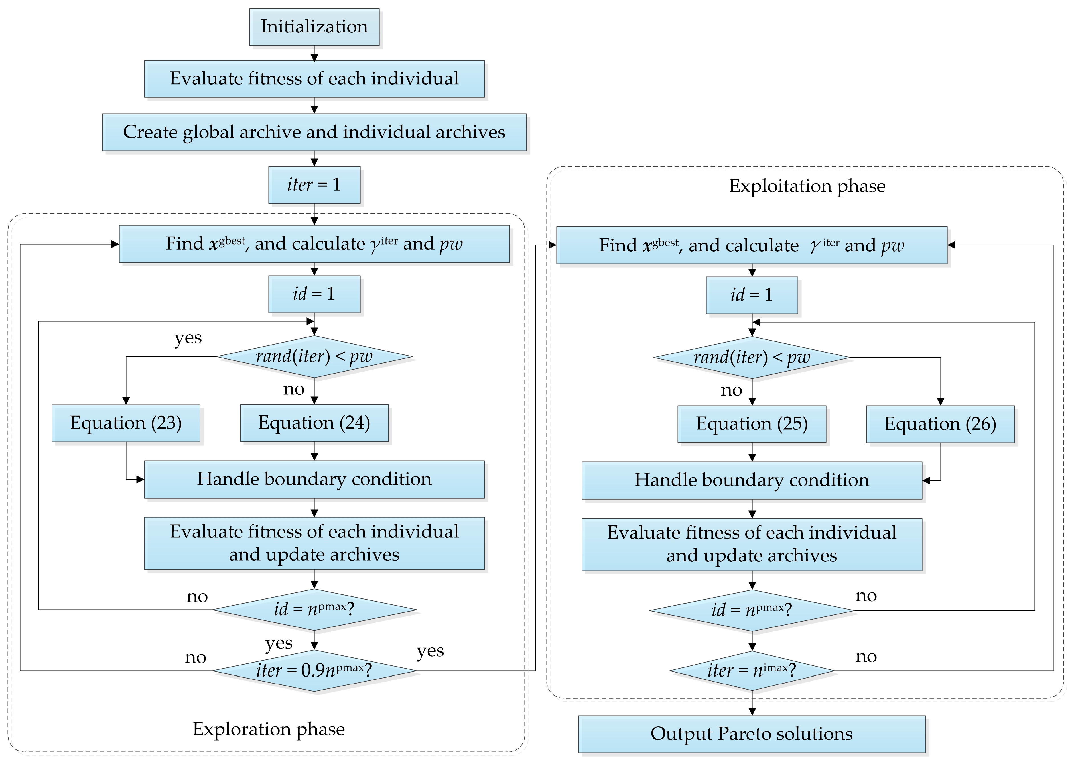
In order to overcome these limits, we propose an offline multi-point trajectory planning technique for manipulators based on quintic non-uniform B-splines and a constrained multi-objective dream optimization algorithm (CMODOA). Quintic non-uniform B-splines with virtual points are utilized for jerk-continuous trajectory, achieving zero values for velocity, acceleration, and jerk at the initial and final motion. CMODOA is a parameter-free algorithm with no specific parameters to be tuned. The proposed algorithm improves and develops the dream optimization algorithm (DOA) via an awakening strategy, an adaptive hyperrectangle, and an adaptive ε-constraint handling method. These enable CMODOA to solve multi-objective optimization problems with various linear and nonlinear constraints. The main contributions of this paper can be summarized as follows:

• The boundary constraints of the optimal problem are transformed into equations for coefficient matrix calculation in the trajectory model based on quintic non-uniform B-splines. Additionally, the normalized knot vector maintains consistency among different joints to satisfy synchronization constraints. The transformation and maintenance significantly reduce the computational complexity during optimization.
• An awakening strategy with a differential mutation is designed to enhance the global search ability of DOA and the diversity of optimization results from DOA. The strategy mimics the phenomenon where people may be awakened by disturbances, leading to interruption of dream continuity. As the sleep duration increases, the probability of being awakened tends to zero.
• An adaptive hyperrectangle is strategically designed to conduct an intensive exploration within the neighbourhood, centred on the dream of the best individual in the global archive. The hyperrectangle serves as a value space for the variables exceeding the boundary condition. The activity coefficient within the hyperrectangle exhibits a nonlinear decay with increasing iterations.
• A constrained non-dominated sorting approach is proposed for the population to explore the relaxed boundary between the feasible solution region and the infeasible solution region. This can enhance optimization algorithms’ ability to conduct an in-depth exploration of the feasible and optimal solutions.

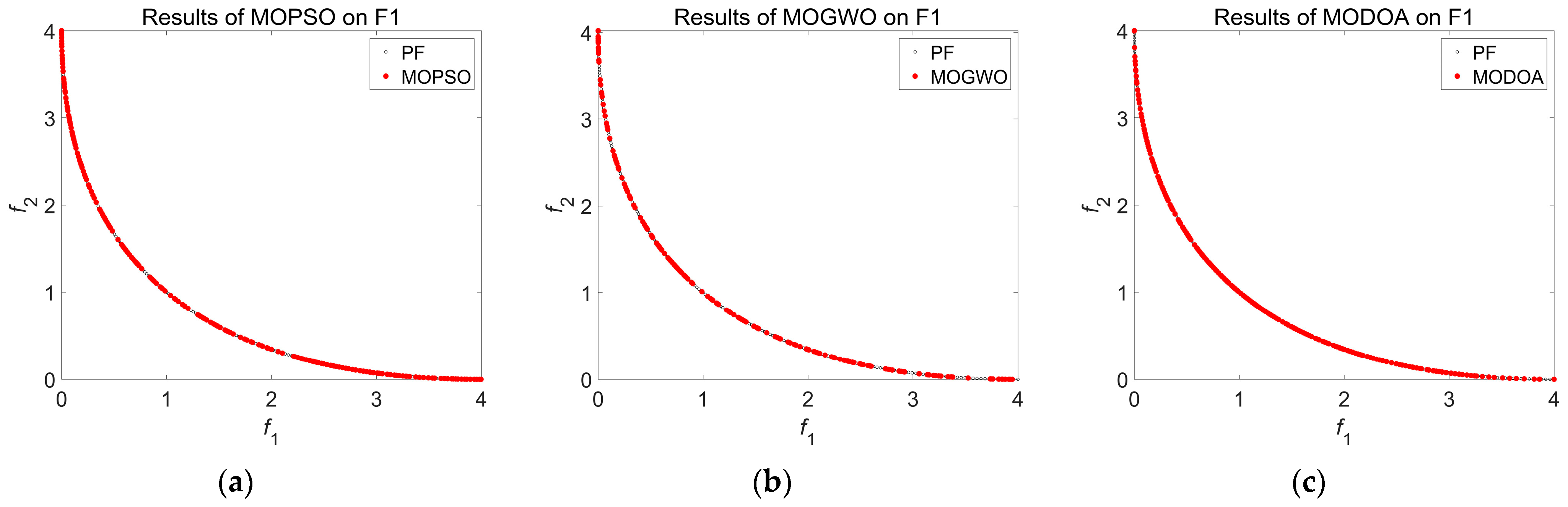
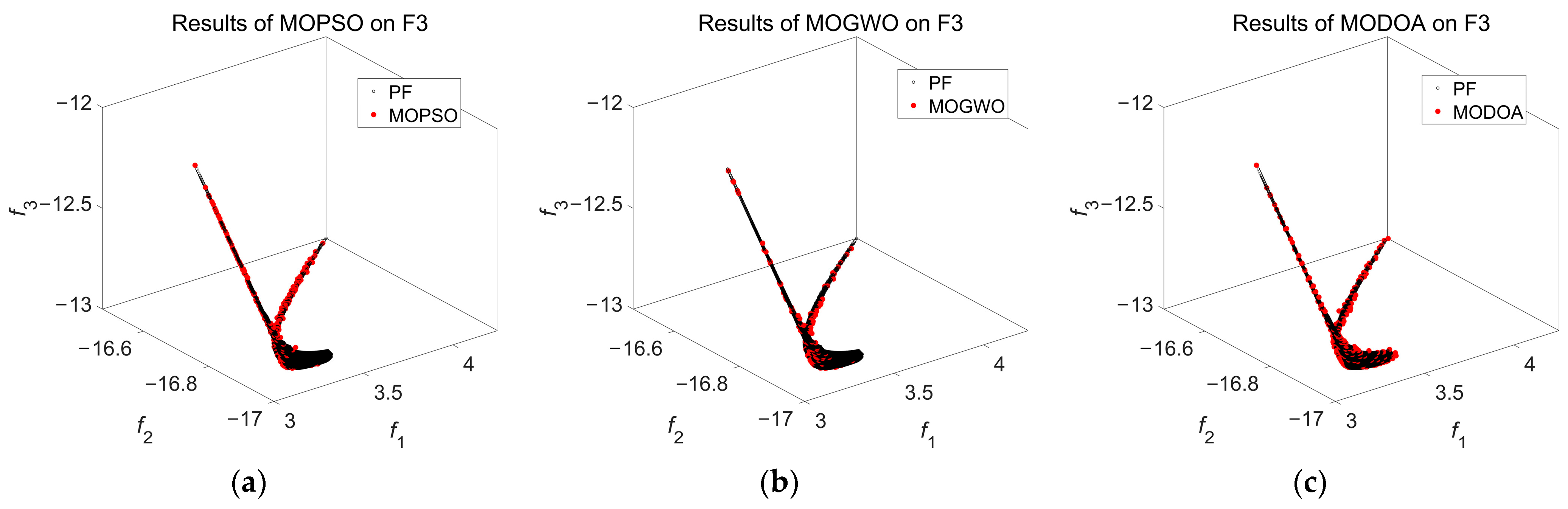
The remaining sections of this article are organized as follows. In Section 2, the problem statement of the time-jerk optimal trajectories is detailed. Section 3 introduces the trajectory model based on quintic non-uniform B-splines with virtual points. In Section 4, the proposed multi-objective optimization algorithm is developed, with two phases. Section 5 presents comparisons with various multi-objective optimization algorithms for test functions, which use different trajectory planning methods for manipulators. Finally, Section 6 concludes this work.

2. Time–Jerk Optimal Problem Statement

The objective of manipulator trajectory optimization is to generate a motion plan that enables the manipulator to transition smoothly from its initial configuration to the final configuration within the operational workspace, while concurrently enhancing system performance through the systematic consideration of various constraints. A minimum-time trajectory can significantly enhance the operational efficiency of a manipulator, enabling rapid response and maximizing task throughput in dynamic environments. However, faster motions may induce significantly stronger jerk loads [1]. Therefore, it is desirable to have sufficiently smooth trajectories to avoid excessive mechanical vibrations. A minimum-jerk trajectory can effectively reduce vibrations and mechanical shocks during manipulator motion, thereby enhancing trajectory tracking precision and overall system stability. The travelling time and the absolute mean jerk are formulated as the two objective functions in this study. The definition of the time-jerk optimization problem is similar to that presented in Ref. [12].

The objective function equations are defined as follows.:

$$\mathrm{Minimum}\mathrm{time}:f_1={\displaystyle \sum _{i=1}^{np-1}\Delta t_i}.$$

(1)

$$\mathrm{Minimum}\mathrm{jerk}:f_2={\displaystyle \sum _{g=1}^{nj}\sqrt{\frac{1}{T}{\displaystyle {\int }_0^T\left(jer{k}_{\mathrm{g}}{\left(t\right)}^2\right)dt}}}.$$

(2)

where Δt_i is the time interval between desired adjacent waypoints, np denotes the number of desired waypoints, jerk_g is the gth joint jerk, T represents the travelling time of an entire manipulator movement, and nj is the number of the utilized manipulator joints. f₁ denotes the travelling time of the manipulator to accomplish a predetermine task, and minimal travelling time implies high motion efficiency. f₂ represents the optimization objective of the absolute mean jerk, indicating the smoothness of the optimized trajectories.

When the kinematic quantities exceed the physical limits of their manipulators, issues like structural damage, control failure, energy surge, intensified vibration, and safety hazards may emerge, significantly compromising system performance and operational safety. Therefore, the optimized trajectory should be subject to the kinematic constraints, defined as follows:

$$\mathrm{Kinematic}\mathrm{constraints}:\left\{\begin{array}{l}\mathrm{velocity}:\left|ve{l}_g(t)\right|\le v{c}_g\\ \mathrm{acceleration}:\left|ac{c}_g(t)\right|\le a{c}_g\\ \mathrm{jerk}:\left|jer{k}_g(t)\right|\le j{c}_g\end{array}\right..$$

(3)

where vel_g and acc_g are the velocity and acceleration of the gth joint, respectively. vc_g, ac_g, and jc_g are the constraints of velocity, acceleration, and jerk for the gth joint, respectively.

The optimized trajectory should also adhere to geometric constraints, ensuring collision-free motion within feasible workspaces and enhancing the reliability of motion planning. The imposed geometric constraints on the joint positions are described as follows:

$$\mathrm{Geometric}\mathrm{constraints}:ang{l}_g^{\min }\le ang{l}_g(t)\le ang{l}_g^{\max }.$$

(4)

where angl_g is the gth joint angle; $ang{l}_g^{\min }$ and $ang{l}_g^{\max }$ are the minimum and maximum of the gth joint angle.

Multi-point joint trajectory planning requires synchronization across all joints. Each joint must start from the initial desired waypoint at the same time, and then sequentially and simultaneously reach every desired waypoint before terminating concurrently at the final desired waypoints. The synchronization constraints are described as follows:

$$\mathrm{Synchronization}\mathrm{constraints}:ang{l}_g({\displaystyle \sum _{m=0}^i\Delta t_i})=p_{g,i},g=1,2,\cdots ,nj,i=0,1,\dots ,np.$$

(5)

where p_g,i is the ith desired waypoint of the gth joint.

In order to prevent abrupt changes and enhance trajectory smoothness and system stability at both the initial and final movements, we suppose that the values of velocity, acceleration, and jerk of all joints at the initial and final movements are zero. The boundary constraints, including velocity, acceleration, and jerk, are described as follows:

$$\mathrm{Boundary}\mathrm{constraints}:\left\{\begin{array}{l}\mathrm{velocity}:ve{l}_g(t=0)=0,ve{l}_g(t=T)=0\\ \mathrm{acceleration}:ac{c}_g(t=0)=0,ac{c}_g(t=T)=0\\ \mathrm{jerk}:jer{k}_g(t=0)=0,jer{k}_g(t=T)=0\end{array}\right..$$

(6)

In addition to the above constraints, torque constraint is a core dynamic constraint, determining the robot motion performance and trajectory feasibility, defined as follows:

$$\mathrm{Torque}\mathrm{constraints}:\left|{\tau }_g\right|\le {\tau }_g^{\max },g=1,2,\cdots ,nj.$$

(7)

where τ_g is the torque of the gth joint and ${\tau }_g^{\max }$ is the torque limit of the gth joint.

For a given manipulator task, initial joint trajectories are generated via trajectory model interpolation. Then, the joint trajectories are optimized by solving the time-jerk optimal problem via multi-objective optimization algorithms and constraint handling techniques. We will ultimately obtain a Pareto solution set that is available for user selection.

3. Trajectory Model Based on Quintic Non-Uniform B-Splines with Virtual Points

Quintic non-uniform B-splines utilize their fifth-degree polynomial formulation to achieve C⁴ continuity, enabling the generation of ultra-smooth motion profiles that effectively reduce component wear and mitigate mechanical shocks during trajectory execution. In addition, the local support characteristic ensures that a knot modification only influences localized trajectory segments, enabling extension of trajectory planning methodologies to dynamic mission scenarios. These unique properties establish quintic non-uniform B-splines as the optimal interpolation solution for manipulator trajectory, particularly excelling in scenarios demanding highly efficient and high-precision tasks with kinematic constraint satisfaction.

A quintic non-uniform B-spline function can be expressed mathematically as follows:

$$angl(u)={\displaystyle \sum _{i=0}^{ncp}{q}_i{N}_{i,5}(u)}$$

(8)

where u is the normalized knot vector variable, q_i is the i-th control point, and ncp is the number of control points. N_i,5(u) denotes the ith basis function of the quintic non-uniform B-spline and can be obtained by the Cox-De Boor recursion algorithm, presented as follows:

$$\left\{\begin{array}{l}{N}_{i,0}(u)=\left\{\begin{array}{l}1,\mathrm{if}{u}_i\le u<u_{i+1}\\ 0,\mathrm{others}\end{array}\right.\\ N_{i,k}(u)={\displaystyle \frac{u-u_i}{u_{i+k}-u_i}}{N}_{i,k-1}(u)+{\displaystyle \frac{u_{i+k-1}-u}{u_{i+k-1}-u_{i+1}}}{N}_{i+1,k-1}(u)\\ \mathrm{define}{\displaystyle \frac{0}{0}}=0\end{array}\right..$$

(9)

In order to satisfy the jerk boundary constraint, two virtual points are inserted into the second and penultimate locations of the desired waypoint sequence. Then, Equation (8) is converted to the following:

$$p_i=\left\{\begin{array}{l}angl(u_5)={\displaystyle \sum _{g=0}^5{q}_g{N}_{g,5}(u_5)},i=0\\ angl(u_{i+5})={\displaystyle \sum _{g=i+1}^{i+6}{q}_g{N}_{g,5}(u_{i+6})},i=1,2,\dots ,np-1\\ angl(u_{np+5})={\displaystyle \sum _{g=np+2}^{np+7}{q}_g{N}_{g,5}(u_{np+7})},i=np\end{array}\right..$$

(10)

Furthermore, in order to respect the synchronization constraint, the normalized knot vector u is calculated from the sequence of time intervals Δt_i, given as follows:

$$\mathit{u}=[u_0,u_1,\dots ,u_{np+10}],$$

(11)

where

$$\left\{\begin{array}{l}{u}_0=u_1=\dots =u_5=0\\ u_i=u_{i-1}+|\Delta t_{i-5}|/{\displaystyle \sum _{g=0}^{np-1}|\Delta t_g|,i=6,\dots ,np+4}\\ u_{np+5}=u_{np+6}=\dots =u_{np+10}=1\end{array}\right..$$

(12)

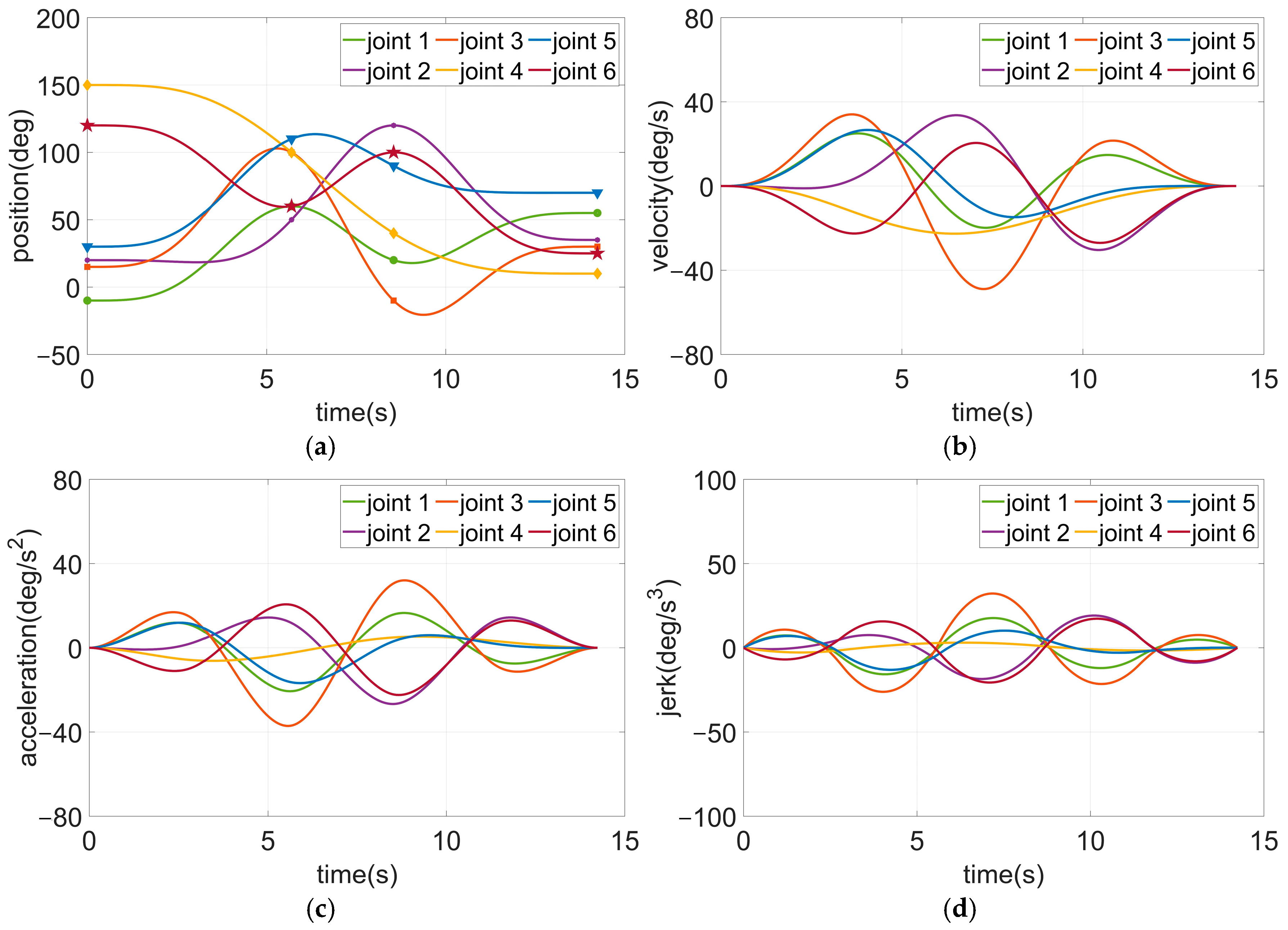
The velocity, acceleration, and jerk are the first-, second-, and third-order derivatives of quintic non-uniform B-spline, respectively:

$$ang{l}^m(u)={\displaystyle \sum _{g=i-5+m}^i{q}_g^m{N}_{g,5-m}(u)},i=0,1,\dots ,np+1$$

(13)

where

$$q_g^m=\left\{\begin{array}{l}{q}_g=,m=0\\ (6-m){\displaystyle \frac{d_g^{m-1}-d_{g-1}^{m-1}}{u_{g+6-m}-u_g}},m=1,2,\dots ,r;g=i-5+m,\dots ,i\end{array}\right.$$

(14)

According to Equations (8) and (9), the boundary constraints can be converted into

$$\left\{\begin{array}{l}vel(t=0)=ang{l}^1(u_5)=q_1^1=0\\ vel(t=T)=ang{l}^1(u_{np+5})=q_{np+4}^1=0\\ acc(t=0)=ang{l}^2(u_5)=q_2^2=0\\ acc(t=T)=ang{l}^2(u_{np+5})=q_{np+4}^2=0\\ jerk(t=0)=ang{l}^3(u_5)=q_3^3=0\\ jerk(t=T)=ang{l}^3(u_{np+5})=q_{np+4}^3=0\end{array}\right..$$

(15)

np + 7 linear equations for control point q can be obtained from Equations (10) and (15):

$$\mathit{q}={\mathit{A}}^{-1}\mathit{B}$$

(16)

where A is a non-singular coefficient matrix determined by Δt_i and can be calculated by Equations (9), (11), and (12).

$$\mathit{A}=\left[\begin{array}{cccccccccc}1& 0& & & & \dots & & & & 0\\ 0& 0& N_{3,5}(u_7)& N_{4,5}(u_7)& N_{5,5}(u_7)& N_{6,5}(u_7)& N_{7,5}(u_7)& 0& \dots & 0\\ ⋮& \ddots & \ddots & \ddots & \ddots & \ddots & \ddots & \ddots & \ddots & ⋮\\ 0& \dots & 0& N_{np+1,5}(u_{np+5})& N_{np+2,5}(u_{np+6})& N_{np+3,5}(u_{np+7})& N_{np+4,5}(u_{np+8})& N_{np+5,5}(u_{np+9})& 0& 0\\ 0& & & & \dots & & & & 0& 1\\ 1& -1& 0& & & \dots & & & & 0\\ 0& & & & \dots & & & 0& -1& 1\\ 0& 1& -1& 0& & & \dots & & & 0\\ 0& & & \dots & & & 0& -1& 1& 0\\ 0& 0& 1& -1& 0& & \dots & & & 0\\ 0& 0& 0& & & 0& -1& 1& 0& 0\end{array}\right]$$

(17)

It can be seen that A is the same for all joints, due to the independence of desired waypoints. B is a coefficient matrix of synchronization constraints and boundary constraints, presented as follows:

$$\mathit{B}={[p_0,p_1,\dots ,p_{np},0,0,0,0,0,0]}^{\mathrm{T}}$$

(18)

After obtaining the control point q through reverse calculation, the initial trajectory can be calculated using Equations (8) and (13). However, the scope of the domain of the trajectory is [0,1], and it is necessary to scale the trajectory to the given travelling time. The scaled trajectory can be calculated by

$$\left\{\begin{array}{c}angl(t)=angl(Tu)=angl(u)\\ vel(t)=vel(Tu)={\displaystyle \frac{1}{T}}vel(u)\\ acc(t)=acc(Tu)={\displaystyle \frac{1}{T^2}}acc(u)\\ jerk(t)=jerk(Tu)={\displaystyle \frac{1}{T^3}}jerk(u)\end{array}\right..$$

(19)

For a specific manipulator task, the multi-point trajectories interpolated by the quintic non-uniform B-splines with virtual points can be immediately calculated to achieve jerk continuity, if Δt_i (i = 1, …, np − 1) is provided.

4. Constrained Multi-Objective Dream Optimization Algorithm

In this section, the proposed constrained multi-objective dream optimization algorithm (CMODOA) is utilized to solve the time-jerk optimal trajectory planning problem of manipulators. CMODOA is primarily composed of a multi-objective dream optimization algorithm and constraint handling techniques.

4.1. Multi-Objective Dream Optimization Algorithm

Dream Optimization Algorithm (DOA) proposed by Lang and Gao in 2025 is a metaheuristic optimization algorithm inspired by human dreams [31]. DOA employs a forgetting-supplementation mechanism to balance exploration and exploitation, together with a dream-sharing strategy and a foundational memory strategy to enhance the ability to escape local optimal solutions. The population from DOA is divided into five groups based on differences in memory capacity, with individuals within each group exhibiting consistent memory, which may weaken population diversity. Moreover, the dream-sharing strategy allows individuals to randomly acquire positional information from others in the forgetting dimension. This strategy enhances the ability to escape local optima, but the global search capability still needs improvement. To further enhance the global search capability of DOA and the diversity of optimization results from DOA, we introduced an awakening strategy and differential mutation to improve the algorithm. In addition, multi-objective DOA (MODOA) was developed based on fast nondominated sorting approach [32] and archive update mechanism to solve multi-objective optimization problems. The flowchart of the proposed MODOA is shown in Figure 1.

4.1.1. Improved Dream Optimization Algorithm

During the initialization phase, the proposed IDOA first generates a random population within the search space as the initial population. The generation for the initial population is as follows:

$${\mathit{x}}_i={\mathit{x}}^{\mathrm{lb}}+\mathit{rand}\times \left({\mathit{x}}^{\mathrm{ub}}-{\mathit{x}}^{\mathrm{lb}}\right),i=1,2,\dots ,n^{\mathrm{pop}}$$

(20)

where n^pop represents the number of individuals, i.e., the population size, x_i denotes the i-th individual in the population, x^lb and x^ub indicate the lower and upper boundaries of the search space, respectively, and rand is a (np − 1) × 1 vector where each dimension is a random number between 0 and 1.

IDOA divides the search process into exploration and exploitation phases. Different individuals may wake up from their sleep due to differences in their physical constitution. An awakening strategy is proposed to describe this mechanism. The probability of waking up is relatively high in the early stages of sleep and decreases nonlinearly as the number of iterations increases. The probability of waking up pw is defined as follows:

$$pw={\displaystyle \frac{1}{5}}\left(1-\cos \left(\pi \left(1-{\gamma }^{\mathrm{iter}}\right)\right)\right)+{\displaystyle \frac{3}{5}}\left(1-{\displaystyle \frac{1}{1+e^{\left(10-20{\gamma }^{\mathrm{iter}}\right)}}}\right)$$

(21)

where γ^iter is the ratio of the current iteration to the maximum iteration.

$${\gamma }^{\mathrm{iter}}={\displaystyle \frac{iter}{n^{\mathrm{imax}}}}$$

(22)

In the exploration phase, iterations range from 0 to 0.9 n^imax, where n^imax is the maximum iteration. After waking up, the continuity of the individual’s dream is weak, and the dream may be influenced by that of the best individual and a random individual. Differential mutation is adopted to update the individual’s dream due to its efficient global search capacity through vector differential perturbation and its applicability for solving high-dimensional nonlinear optimization problems.

$${\mathit{x}}_i^{iter+1}={\mathit{rand}}_1\times ({\mathit{x}}_{\mathrm{gbest}}^{iter}-{\mathit{x}}_i^{iter})+{\mathit{rand}}_2\times ({\mathit{x}}_{\mathrm{rand}}^{iter}-{\mathit{x}}_i^{iter})$$

(23)

where ${\mathit{x}}_i^{iter}$ denotes the i-th individual at the iter-th iteration; ${\mathit{x}}_{\mathrm{gbest}}^{iter}$ and ${\mathit{x}}_{\mathrm{rand}}^{iter}$ are the global best and random individuals at the iter-th iteration, respectively; and rand₁ and rand₂ are different dim-dimensional vectors where each dimension is a random number between 0 and 1. The individual with the maximum density in the global archive is selected as the global best one, and the details of the individual density calculations are shown in Section 4.1.2.

In the absence of waking up, the individual’s dream will perform forgetting and supplementation based on the individual’s historical best dream. The forgetting and supplementation strategy combines global and local search capacities, allowing the individual to forget and self-organize information. The updated formula is as follows:

$${\mathit{x}}_i^{iter+1}={\mathit{x}}_i^{\mathrm{lbest}}+{\displaystyle \frac{1}{2}}\left({\mathit{x}}^{\mathrm{lb}}+\mathit{rand}\times \left({\mathit{x}}^{\mathrm{ub}}-{\mathit{x}}^{\mathrm{lb}}\right)\right)\left(\cos \left(\pi \times {\displaystyle \frac{10iter+n^{\mathrm{imax}}}{10n^{\mathrm{imax}}}}\right)+1\right).$$

(24)

where ${\mathit{x}}_i^{\mathrm{lbest}}$ is the historical best dream of the i-th individual. Similar to the method of finding the global best individual, the individual with the maximum density in the corresponding individual archive is selected as the historical best dream.

In the exploitation phase, iterations range from 0.9 n^imax to n^imax. In contrast to the exploration phase, individuals retain more dream information due to the longer duration of sleep. After waking up, the continuity of the individual’s dream is strong, and the dream may be influenced by the dream of the best individual in the global archive and the historical best dream of the individual.

$${\mathit{x}}_i^{iter+1}={\mathit{x}}_i^{iter}+{\mathit{rand}}_1\times \left({\mathit{x}}_{\mathrm{gbest}}^{iter}-{\mathit{x}}_i^{iter}\right)+{\mathit{rand}}_2\times \left({\mathit{x}}_i^{\mathrm{lbest}}-{\mathit{x}}_i^{iter}\right)$$

(25)

In the absence of waking up, the individual’s dream will move continuously towards the dream of the best individual in the global archive while implementing the forgetting and supplementation strategy.

$${\mathit{x}}_i^{iter+1}={\mathit{x}}_{\mathrm{gbest}}^{iter}+{\displaystyle \frac{1}{2}}\left({\mathit{x}}^{\mathrm{lb}}+\mathit{rand}\times \left({\mathit{x}}^{\mathrm{ub}}-{\mathit{x}}^{\mathrm{lb}}\right)\right)\left(\cos \left(\pi \times {\displaystyle \frac{iter}{n^{\mathrm{imax}}}}\right)+1\right)$$

(26)

Equation (24) shows that individuals conduct exploitation in a smaller domain centred on the dream of the best individual in the global archive and regenerate information while dreaming.

4.1.2. Boundary Condition Handling

Some variable values of the updated individual may exceed the predefined domain. In this case, a boundary condition handling is utilized to ensure that these variables maintain their values within the domain. Although the awakening strategy with differential mutation can increase the global search ability of the DOA, it may reduce the convergence of the algorithm. In order to fully utilize the neighbourhood of the dream of the best individual in the global archive for enhanced convergence, we proposed an adaptive hyperrectangle of the dream of the best individual in the global archive as a value space for these variables, as shown below:

$${\mathit{x}}_i^{iter+1}=\mathit{lg}\times {\mathit{x}}_i^{iter}+\neg \mathit{lg}\times \left({\mathit{x}}_{\mathrm{gbest}}^{iter}+{\mathit{r}}_1\times \underset{\mathrm{adaptive}\mathrm{hyperrectangle}}{\underbrace{{\gamma }^{\mathrm{bc}}\times \min \left\{{\mathit{x}}_{\mathrm{gbest}}^{iter}-{\mathit{x}}^{\mathrm{lb}},{\mathit{x}}^{\mathrm{ub}}-{\mathit{x}}_{\mathrm{gbest}}^{iter}\right\}}}\right).$$

(27)

where lg and ¬lg are (np − 1) × 1 vectors where each dimension is a number of 0 or 1. When the variable value in a dimension of an individual is not within the predefined domain, the value of lg in that dimension is taken as 0. Otherwise, the value is taken as 1. The value assignment of ¬lg is exactly the opposite of lg. r₁ is a (np − 1) × 1 vector where each dimension is a random number of 1 or −1. γ^bc is an activity coefficient of the dream of the best individual in the global archive and nonlinearly decreases as the number of iterations increases.

$${\gamma }^{\mathrm{bc}}=e^{-{\left(3{\gamma }^{\mathrm{iter}}\right)}^2}$$

(28)

The edge length of each side of the hyperrectangle is defined as being twice that of the smaller distances from the variable value of each dimension of the dream of the best individual in the global archive to the upper and lower bounds. Figure 2 shows a schematic diagram of an adaptive hyperrectangle of the dream of the best individual in the global archive. The green solid lines represent the shorter distance from the variable value of each dimension of the dream of the best individual in the global archive to the upper and lower bounds. The pink rectangle is the resulting adaptive hyperrectangle.

4.1.3. Archive Update Mechanism

A global archive is utilized to store the non-dominated Pareto solutions found so far. Before finding non-dominated Pareto solutions during the iteration process, the global archive is an empty set. The storage size of the global archive, denoted as n^armax, needs to be predefined and has a finite value. After each iteration, MODOA may generate new non-dominated Pareto solutions. These new solutions may be dominated by the Pareto solutions in the global archive, or they may dominate some or all of the existing Pareto solutions in the global archive. Furthermore, if the number of non-dominated Pareto solutions found so far exceeds n^armax, it is necessary to perform an updated operation for the individuals in the global archive to maintain the storage size within the predefined limit.

The global archive update mechanism is employed to regulate the newly generated non-dominated Pareto solutions and the existing Pareto solutions in the global archive. This process involves removing the dominated Pareto solutions, thereby forming a new set of non-dominated Pareto solutions, while ensuring that the storage space remains within the predefined limit. The rules for global archive update mechanism are outlined below:

• If all the newly generated non-dominated Pareto solutions are dominated by the Pareto solutions in the global archive, these new solutions are not allowed to be added to the global archive.
• If only some of the newly generated non-dominated Pareto solutions are dominated by the Pareto solutions in the global archive, then the remaining new solutions that are not dominated by the Pareto solutions in the global archive are allowed to be added to the global archive.
• If all or some of the Pareto solutions in the global archive are dominated by the newly generated non-dominated Pareto solutions, then the dominated Pareto solutions are removed from the global archive, and the new non-dominated Pareto solutions are added to the global archive.
• If there is no dominance relationship between the newly generated non-dominated Pareto solutions and the Pareto solutions in the global archive (i.e., they are mutually non-dominating), then the new non-dominated Pareto solutions are added to the global archive.
• When the size of the integrated population exceeds n^armax, individual density calculation is employed to remove the non-dominated Pareto solutions with lower individual densities until the population size is reduced to n^armax. The resulting set of solutions is then stored in the global archive.

In addition to the global archive, each individual also has its own separate archive to store the individual’s historical best dream. The size of this individual archive always remains 1. After each iteration, the updated dream is compared to the historical best dream in its archive. If the density of the updated dream is greater than the historical best dream, then the historical best dream is replaced by the updated dream.

4.1.4. Density Calculation

Static weights neglect the stage-dependent disparity between the structural properties of decision space and the convergence requirements in objective space, thereby diminishing the distribution diversity of the population in either space. Concurrently, they may misguide search directions, impeding algorithms from approximating the true Pareto front and degrading convergence efficiency. In contrast, dynamic weights effectively strike a dynamic balance between the convergence and diversity of solutions, particularly in complex high-dimensional scenarios. Therefore, an individual density calculation method based on dynamic weighting is proposed to enhance the distribution diversity of the population in both the decision space and the objective space, and to filter out individuals with lower density in these spaces, while providing a theoretical basis for selecting the global and historical best dreams. Normalization is introduced to eliminate the influence of different orders of magnitude in the two spaces.

The density of individuals in the decision space D^x(i) can be calculated using several neighbouring individuals along the variable axis, as follows:

$$D^{\mathrm{x}}(i)=\left\{\begin{array}{c}1,\mathrm{if}i=1\mathrm{or}i=n^{\mathrm{pop}}\\ {\displaystyle \prod _{j=1}^{nx}\frac{x_{j,i+1}-x_{j,i-1}}{x_j^{\max }-x_j^{\min }}},\mathrm{others}\end{array}\right.$$

(29)

where nx represents the variable dimension and n^pop represents the number of individuals to be compared.

The density of individuals in the objective space D^f(i) can be calculated using two neighbouring individuals along the non-dominated front, as follows:

$$D^{\mathrm{f}}(i)=\left\{\begin{array}{c}1,\mathrm{if}i=1\mathrm{or}i=n^{\mathrm{pop}}\\ {\displaystyle \prod _{j=1}^{nf}\frac{f_{j,i+1}-f_{j,i-1}}{f_j^{\max }-f_j^{\min }}},\mathrm{others}\end{array}\right.$$

(30)

where nf represents the objective dimension.

During the early iterations, individuals in the population should be distributed as widely as possible in the decision space to enhance the exploration capability of MODOA. In the later iterations, individuals in the population should be distributed as widely as possible in the objective space and be close to the Pareto optimal front to improve the convergence ability of MODOA. Thus, dynamic weights that vary with each iteration are introduced when evaluating individual density. The total density of an individual is equal to the weighted sum of the individual density in the decision and objective spaces, as follows:

$$D(i)=\left(2-{\displaystyle \frac{2}{1+e^{\left(-10{\gamma }^{\mathrm{iter}}\right)}}}\right)\times D^{\mathrm{x}}(i)+\left({\displaystyle \frac{2}{{1+\mathit{e}}^{\left(-10{\gamma }^{\mathrm{iter}}\right)}}}-1\right)\times D^{\mathrm{f}}(i)$$

(31)

The weight of the density of individuals in the decision space decreases as the number of iterations increases, while the weight in the objective space increases accordingly.

4.2. Constraint Handling Techniques

A multi-objective optimization with constraints can be defined as follows:

$$\left\{\begin{array}{c}\min \Phi \left(\mathit{x}\right)=\left({\varphi }_1\left(\mathit{x}\right),{\varphi }_2\left(\mathit{x}\right),\dots ,{\varphi }_l\left(\mathit{x}\right)\right)\\ s.t.{\eta }_g\left(\mathit{x}\right)\le 0,g=1,2,\dots ,m\\ {\psi }_j\left(\mathit{x}\right)=0,j=1,2,\dots ,k\end{array}\right.$$

(32)

where ϕ(x) are objectives, η_i(x) are inequality constraints, ψ_j(x) are equality constraints, and l, m, and k are the number of objectives, inequality constraints, and equality constraints, respectively.

Optimization algorithms may obtain non-feasible solutions for optimization problems with constraints. These solutions do not satisfy the constraints during the optimization process. Constraint handling techniques are employed to address nonlinear or linear constraints in optimization problems, enabling the identification of feasible solutions within the domain of variables. In order to enhance the boundary exploration mechanisms in constraint handling strategies, an adaptive ε-constraint handling method is adopted.

4.2.1. Adaptive ε-Constraint Handling Method

The key idea of this method is to transform infeasible individuals with constraint violation values within an ε-boundary band into relaxed feasible solutions, allowing the population to explore the relaxed boundary between the feasible solution region and the infeasible solution region. This can enhance the optimization algorithms’ ability to conduct an in-depth exploration of the feasible and optimal solutions.

The updated formula of ε is expressed as follows:

$$\epsilon \left({\gamma }^{\mathrm{iter}},{\gamma }^{\mathrm{f}}\right)=\left\{\begin{array}{c}{\displaystyle \frac{1}{1+e^{\left(\frac{1}{1-\min \left({\gamma }^{\mathrm{iter}},{\gamma }^{\mathrm{f}}\right)}-\frac{1}{\min \left({\gamma }^{\mathrm{iter}},{\gamma }^{\mathrm{f}}\right)}\right)}}},iter\le 0.5n^{\mathrm{imax}}\\ {\displaystyle \frac{1}{1+e^{\left(\frac{1}{1-\max \left({\gamma }^{\mathrm{iter}},{\gamma }^{\mathrm{f}}\right)}-\frac{1}{\max \left({\gamma }^{\mathrm{iter}},{\gamma }^{\mathrm{f}}\right)}\right)}}},iter>0.5n^{\mathrm{imax}}\end{array}\right.$$

(33)

where γ^f represents the ratio of feasible solutions to all solutions.

When iter ≤ 0.5 n^imax, the lower value between γ^iter and γ^f is selected to calculate ε, maintaining the exploration of a population in a larger area. This allows the population to be closer to the Pareto frontier, preventing it from becoming trapped in local optima. When iter > 0.5 n^imax, the larger value between γ^iter and γ^f is chosen to generate ε, achieving the convergence of optimization algorithms and preserving the diversity of the Pareto optimal solution set in archives. ε is continuously updated until the iteration reaches the termination condition, and its value changes with γ^iter and γ^f, as illustrated in Figure 3.

After an iteration, individuals in the population are classified into three sets: the feasible solution set S^f, the relaxed solution set S^r, and the infeasible solution set S^if. The selection criteria for the relaxed solution set are jointly determined by ε, the population size, and the constraint violation values of the infeasible solutions within the population. When the constraint violation value of an individual is less than or equal to sc(iter), the individual is classified into the relaxed solution set. sc(iter) is defined as follows:

$$sc\left(iter\right)={\displaystyle \frac{\epsilon \left(iter\right){\displaystyle \sum _{i=1}^{n^{\mathrm{pmax}}}vv\left(i\right)}}{n^{\mathrm{pmax}}}}$$

(34)

where vv(i) represents the constraint violation value of the ith individual, calculated using the following formula:

$$vv\left(i\right)={\displaystyle \sum _{g=1}^m\max \left\{0,\left|{\eta }_g\left({\mathit{x}}_i\right)\right|\right\}}+{\displaystyle \sum _{j=1}^k\left|{\psi }_j\left({\mathit{x}}_i\right)\right|}$$

(35)

The constraint violation value of an individual is also utilized to perform constrained non-dominated sorting.

4.2.2. Constrained Non-Dominated Sorting

In order to further compare the infeasible solutions, a constrained non-dominated sorting approach is proposed in this paper. A solution, x₁, is said to dominate another solution, x₂, when any of the following conditions is met:

• If x₁, x₂ ∈ S^f, x₁ is Pareto-dominated x₂.
• If x₁, x₂ ∈ S^f and they have the same nondomination rank, D(x₁) > D(x₂).
• x₁ ∈ S^f and x₂ ∈ S^r or x₂ ∈S^if.
• If x₁, x₂ ∈ S^r, only compare their finesses. x₁ is Pareto-dominated x₂, or they have the same nondomination rank and D(x₁) ≥ D(x₂).
• x₁ ∈ S^r and x₂ ∈S^if.
• If x₁, x₂ ∈ S^if, vv(x₁) ≤ vv(x₂).

The operation flow of CMODOA is similar to that of MODOA, with differences existing in the following three aspects:

(1)

The dream of the best individual in the global archive is selected according to the constrained non-dominated sorting approach;

(2)

The historical best dream of an individual is also selected according to the constrained non-dominated sorting approach and is added to its individual archive, regardless of whether the individual is an infeasible solution;

(3)

Only feasible solutions can be added to the global archive.

5. Simulation Results and Discussion

In order to validate the effectiveness of the proposed MODOA and trajectory planning based on CMODOA, three classical test functions and two typical multi-point trajectory tasks for 6-DOF manipulators were conducted. All the simulations were run on a personal computer with an operating system of Windows 10 64-bit, a CPU of Intel Core i7-13700 KF, and an RAM of 32.0 GB.

5.1. Performance Verification of MODOA

The details of three classical test functions are shown in

Table 1. Multi-objective benchmark problems.

Problem	Variable Bounds	Objective Functions	Features of PF
F1	x ∈ [−5,5]	$\begin{array}{l}{f}_1(x)=x^2\\ f_2(x)={\left(x-2\right)}^2\end{array}$	Convex
F2	x1 ∈ [−1,1], x2 ∈ [0,2]	$\begin{array}{l}{f}_1(x)=\left|x_1\right|\\ f_2(x)=1-x_1^2+2x_2-\sin {\left(\pi \left|x_1\right|\right)}^2\end{array}$	Concave
F3	x1, x2 ∈ [−4,4]	$\begin{array}{l}{f}_1(x)={\displaystyle \frac{1}{2}}{\left(x_1-2\right)}^2+{\displaystyle \frac{1}{13}}{\left(x_2+1\right)}^2+3\\ f_2(x)={\displaystyle \frac{1}{36}}{\left(x_1+x_2-3\right)}^2+{\displaystyle \frac{1}{8}}{\left(-x_1+x_2+2\right)}^2-17\\ f_3(x)={\displaystyle \frac{1}{175}}{\left(x_1+2x_2-1\right)}^2+{\displaystyle \frac{1}{17}}{\left(-x_1+2x_2\right)}^2-13\end{array}$	Nonconvex, non-concave

. The features of Pareto Frontier (PF) include convex, concave, and none of them. MODOA is compared to multi-objective particle swarm optimization (MOPSO) [33] and multi-objective grey wolf optimizer (MOGWO) [34]. No specific parameters need to be tuned for MODOA. The specific parameter configurations of MOPSO and MOGWO are shown in

Table 2. Specific parameter configurations of MOPSO and MOGWO.

Algorithm	Parameter	Value
MOPSO [33]	Inertia weight	0.4
	Individual confidence factor	1
	Swarm confidence factor	1
	Number of grids in each dimension	30
	Uniform mutation percentage	0.5
MOGWO [34]	Grid inflation parameter	0.1
	Number of grids per each dimension	10
	Leader selection pressure parameter	4
	Extra repository member selection pressure	2

. The general parameters of these algorithms are set as follows: the population size n^pop = 200, the archive size n^armax = 200, and the maximum iteration n^imax = 100. In addition, an ablation study was conducted to verify the individual contributions of MODOA components. On the basis of MODOA, the proposed density calculation was replaced with the crowding distance calculation for MODOA_I, the boundary condition handling method was consistent with that in the original DOA for MODOA_II, and the awakening strategy with differential mutation was replaced with the memory strategy and the dream-sharing strategy in the original DOA for MODOA_III.

For the performance metrics, we utilize generational distance (GD), hypervolume (HV), spacing (SP), spread (SD), and run time (RT) to evaluate the performance of MODOA. GD and SD are used to quantify the convergence of solutions. HV represents the volume covered by the solutions. SP is used to measure the coverage of solutions. RT stands for algorithm runtime. The smaller the values of GD, SP, SD, and RT, and the larger the value of HV, the better the performance of an algorithm.

$$GD={\displaystyle \frac{{\left({\displaystyle \sum _{i=1}^{ns}{d}_i}\right)}^{\frac{1}{l}}}{ns}}$$

(36)

$$HV=\Theta \left(\underset{i=1}{\overset{ns}{\cup }}{\lambda }_i\right)$$

(37)

$$SP=\sqrt{{\displaystyle \frac{1}{ns-1}}{{\displaystyle \sum _{i=1}^{ns}\left(\overline{d}-d_i\right)}}^2}$$

(38)

$$SD={\displaystyle \frac{{\displaystyle \sum _{i=1}^{ns-1}\left|\overline{D}-D_i\right|}}{\left(ns-1\right)\overline{D}}}$$

(39)

where ns denotes the number of obtained Pareto solutions, nf denotes the number of true Pareto solutions, Θ represents the Lebesgue measure, λ_i is the hyper-cube from the ith solution and the corresponding reference point, D_i is the Euclidean distance between adjacent solutions, $\overline{D}$ is the average of D_i, and $\overline{d}$ is the average of all d_i. d_i denotes the minimum Euclidean distance between the ith solution and other solutions, defined as follows:

$$d_i=\underset{j}{\min }\left(\left|f_1({\mathit{x}}_i)-f_1({\mathit{x}}_j)\right|+\left|f_2({\mathit{x}}_i)-f_2({\mathit{x}}_j)\right|+\dots +\left|f_l({\mathit{x}}_i)-f_l({\mathit{x}}_j)\right|\right)$$

(40)

Each algorithm is run 500 times on each test problem and the initial population of the three algorithms remains consistent for each run. The statistical results of these 500 runs are shown in

Table 3. Comparisons of GD, HV, SP, SD, and TR metrics for F1.

Metrics		MOPSO [33]	MOGWO [34]	MODOA	MODOA_I 1	MODOA_II 2	MODOA_III 3
GD	Best	5.96 × 10−3	5.93 × 10−3	5.77 × 10−3	5.94 × 10−3	5.85 × 10−3	5.85 × 10−3
	Worst	6.87 × 10−3	6.80 × 10−3	6.61 × 10−3	6.75 × 10−3	6.67 × 10−3	6.61 × 10−3
	Average	6.36 × 10−3	6.36 × 10−3	6.24 × 10−3	6.34 × 10−3	6.24 × 10−3	6.24 × 10−3
	Median	6.36 × 10−3	6.37 × 10−3	6.24 × 10−3	6.34 × 10−3	6.25 × 10−3	6.24 × 10−3
	STD	1.43 × 10−4	1.35 × 10−4	1.33 × 10−4	1.40 × 10−4	1.39 × 10−4	1.30 × 10−4
HV	Best	3.85	3.87	3.84	3.84	3.84	3.85
	Worst	3.83	3.60	3.84	3.84	3.83	3.83
	Average	3.84	3.76	3.84	3.84	3.84	3.84
	Median	3.84	3.76	3.84	3.84	3.84	3.84
	STD	2.07 × 10−3	4.82 × 10−2	1.01 × 10−3	9.83 × 10−4	1.02 × 10−3	9.48 × 10−4
SP	Best	3.50 × 10−1	7.05 × 10−1	4.07 × 10−1	3.12 × 10−1	4.15 × 10−1	3.87 × 10−1
	Worst	5.08 × 10−1	1.02	5.87 × 10−1	4.97 × 10−1	6.02 × 10−1	5.10 × 10−1
	Average	4.19 × 10−1	8.39 × 10−1	4.82 × 10−1	3.88 × 10−1	4.84 × 10−1	4.41 × 10−1
	Median	4.18 × 10−1	8.33 × 10−1	4.79 × 10−1	3.83 × 10−1	4.80 × 10−1	4.41 × 10−1
	STD	2.51 × 10−2	5.24 × 10−2	3.24 × 10−2	3.17 × 10−2	3.35 × 10−2	2.13 × 10−2
SD	Best	8.35 × 10−3	1.21 × 10−2	1.09 × 10−2	9.59 × 10−3	1.32 × 10−2	1.22 × 10−2
	Worst	2.43 × 10−2	2.59 × 10−2	4.10 × 10−2	1.94 × 10−2	3.79 × 10−2	2.31 × 10−2
	Average	1.16 × 10−2	1.86 × 10−2	2.20 × 10−2	1.22 × 10−2	2.16 × 10−2	1.76 × 10−2
	Median	1.13 × 10−2	1.85 × 10−2	2.12 × 10−2	1.19 × 10−2	2.08 × 10−2	1.76 × 10−2
	STD	1.68 × 10−3	2.05 × 10−3	4.77 × 10−3	1.53 × 10−3	4.38 × 10−3	1.75 × 10−3
RT	Best	2.92	7.50 × 101	1.15	1.13	1.21	9.79 × 10−1
	Worst	7.67	1.81 × 102	3.02	2.97	3.19	2.27
	Average	5.27	1.30 × 102	1.86	1.83	1.96	1.55
	Median	6.74	1.69 × 102	2.25	2.19	2.35	1.85
	STD	1.88	4.67 × 10	5.50 × 10−1	5.41 × 10−1	5.89 × 10−1	4.46 × 10−1
Best/All		10/25	1/25	14/25	/	/	/

¹ Density calculation replaced with crowding distance calculation. ² The boundary condition handling is consistent with that in the original DOA. ³ Awakening strategy with differential mutation replaced with the memory strategy and dream-sharing strategy in the original DOA.

,

Table 4. Comparisons of GD, HV, SP, SD, and TR metrics for F2.

Metrics		MOPSO [33]	MOGWO [34]	MODOA	MODOA_I	MODOA_II	MODOA_III
GD	Best	3.34 × 10−3	3.19 × 10−3	3.96 × 10−3	3.06 × 10−3	4.00 × 10−3	3.70 × 10−3
	Worst	4.62 × 10−3	5.58 × 10−3	5.10 × 10−3	6.69 × 10−3	5.09 × 10−3	1.63 × 10−2
	Average	3.78 × 10−3	3.82 × 10−3	4.52 × 10−3	4.37 × 10−3	4.54 × 10−3	6.83 × 10−3
	Median	3.75 × 10−3	3.79 × 10−3	4.53 × 10−3	4.32 × 10−3	4.54 × 10−3	6.43 × 10−3
	STD	2.18 × 10−4	2.87 × 10−4	2.00 × 10−4	5.23 × 10−4	1.93 × 10−4	2.05 × 10−3
HV	Best	1.06 × 10	1.15× 10	1.07× 10	1.52× 10	1.05× 10	1.85× 10
	Worst	8.77	8.79	9.18	8.22	9.21	5.54
	Average	9.82	9.90	9.86	1.10 × 10	9.86	1.01 × 10
	Median	9.82	9.87	9.87	1.04 × 10	9.84	9.9
	STD	2.36 × 10−1	3.47 × 10−1	2.18 × 10−1	1.55	2.42 × 10−1	1.95
SP	Best	4.70 × 10−1	7.47 × 10−1	7.87 × 10−1	6.42 × 10−1	7.86 × 10−1	7.59 × 10−1
	Worst	9.82 × 10−1	1.18	9.49 × 10−1	1.66	9.38 × 10−1	1.37
	Average	7.37 × 10−1	9.37 × 10−1	8.61 × 10−1	9.92 × 10−1	8.60 × 10−1	1.07
	Median	7.36 × 10−1	9.29 × 10−1	8.62 × 10−1	9.56 × 10−1	8.60 × 10−1	1.07
	STD	1.01 × 10−1	7.75 × 10−2	2.83 × 10−2	2.26 × 10−1	2.92 × 10−2	9.95 × 10−2
SD	Best	4.23 × 10−3	6.57 × 10−3	5.96 × 10−3	5.53 × 10−3	5.56 × 10−3	3.32 × 10−3
	Worst	2.35 × 10−2	2.08 × 10−2	1.69 × 10−2	7.28 × 10−2	1.37 × 10−2	9.26 × 10−2
	Average	9.33 × 10−3	1.06 × 10−2	8.40 × 10−3	1.65 × 10−2	8.70 × 10−3	7.40 × 10−3
	Median	8.45 × 10−3	1.04 × 10−2	8.18 × 10−3	1.40 × 10−2	8.54 × 10−3	7.10 × 10−3
	STD	3.15 × 10−3	2.21 × 10−3	1.23 × 10−3	9.24 × 10−3	1.31 × 10−3	4.18 × 10−3
RT	Best	2.19	5.05× 10	7.36 × 10−1	7.36 × 10−1	7.54 × 10−1	5.82 × 10−1
	Worst	8.31	1.36 × 102	1.68	1.77	1.59	1.33
	Average	5.22	1.03 × 102	1.31	1.28	1.31	1.05
	Median	5.68	1.11 × 102	1.39	1.36	1.38	1.11
	STD	1.26	2.16× 10	2.27 × 10−1	2.20 × 10−1	2.25 × 10−1	1.82 × 10−1
Best/All		7/30	4/30	19/30	/	/	/

and

Table 5. Comparisons of GD, HV, SP, SD, and TR metrics for F3.

Metrics		MOPSO [33]	MOGWO [34]	MODOA	MODOA_I	MODOA_II	MODOA_III
GD	Best	4.46 × 10−3	4.19 × 10−3	4.40 × 10−3	4.03 × 10−3	4.46 × 10−3	5.05 × 10−3
	Worst	1.16 × 10−2	3.48 × 10−2	4.76 × 10−3	9.06 × 10−2	1.11 × 10−2	4.67 × 10−2
	Average	6.36 × 10−3	6.60 × 10−3	4.62 × 10−3	6.12 × 10−3	5.56 × 10−3	1.43 × 10−2
	Median	5.95 × 10−3	6.08 × 10−3	4.62 × 10−3	4.96 × 10−3	4.80 × 10−3	1.08 × 10−2
	STD	1.68 × 10−3	2.47 × 10−3	5.22 × 10−5	5.00 × 10−3	1.39 × 10−3	8.87 × 10−3
HV	Best	7.20 × 10−1	7.20 × 10−1	2.40 × 10−1	7.14 × 10−1	7.20 × 10−1	7.59 × 10
	Worst	2.40 × 10−1	2.32 × 10−1	2.40 × 10−1	5.49 × 10−2	2.37 × 10−1	1.88 × 10−1
	Average	3.91 × 10−1	3.73 × 10−1	2.40 × 10−1	2.94 × 10−1	3.29 × 10−1	9.67 × 10−1
	Median	3.42 × 10−1	3.44 × 10−1	2.40 × 10−1	2.48 × 10−1	2.56 × 10−1	4.97 × 10−1
	STD	1.46 × 10−1	1.21 × 10−1	2.23 × 10−5	1.05 × 10−1	1.34 × 10−1	3.48
SP	Best	2.38 × 10−1	6.45 × 10−1	2.76 × 10−1	5.93 × 10−1	2.68 × 10−1	3.71 × 10−1
	Worst	1.11	1.52	3.96 × 10−1	1.71	1.14	1.86
	Average	5.77 × 10−1	1.00	3.26 × 10−1	9.47 × 10−1	4.91 × 10−1	9.46 × 10−1
	Median	4.97 × 10−1	1.01	3.25 × 10−1	8.71 × 10−1	3.55 × 10−1	9.90 × 10−1
	STD	2.80 × 10−1	1.74 × 10−1	2.15 × 10−2	2.37 × 10−1	2.51 × 10−1	3.06 × 10−1
SD	Best	1.77 × 10−3	3.51 × 10−3	2.02 × 10−3	2.57 × 10−3	1.84 × 10−3	2.32 × 10−3
	Worst	1.32 × 10−1	1.39 × 10−1	4.75 × 10−3	1.37 × 10−1	1.41 × 10−1	2.52
	Average	3.23 × 10−2	2.89 × 10−2	2.88 × 10−3	1.32 × 10−2	2.26 × 10−2	4.61 × 10−2
	Median	1.77 × 10−2	1.47 × 10−2	2.85 × 10−3	5.84 × 10−3	4.57 × 10−3	1.86 × 10−2
	STD	3.49 × 10−2	3.03 × 10−2	3.53 × 10−4	2.10 × 10−2	3.28 × 10−2	1.25 × 10−1
RT	Best	1.56	4.42 × 10	1.01	9.97 × 10−1	6.25 × 10−1	6.62 × 10−1
	Worst	4.53	1.26 × 102	2.60	2.51	1.48	2.14
	Average	3.52	9.46 × 10	1.93	1.90	1.13	1.34
	Median	3.92	1.05 × 102	2.07	2.03	1.22	1.39
	STD	9.37 × 10−1	2.26 × 10	3.97 × 10−1	3.90 × 10−1	2.31 × 10−1	3.04 × 10−1
Best/All		8/30	3/30	19/30	/	/	/

, where STD is the standard deviation used to describe the stability of an algorithm.

The results of Table 3, Table 4 and Table 5 show that the overall time consumption of MODOA is relatively longer than that of MODOA_I, MODOA_II, and MODOA_III, but the difference is small. This may be due to the relatively large amount of code caused by the computational complexity of MODOA. For the convex optimization problem, MODOA outperforms MODOA_II in terms of the convergence and coverage of solutions and calculation time, while MODOA has similar performance in terms of the convergence and coverage of solutions compared to MODOA_I, but a weaker performance than MODOA_III. However, MODOA demonstrates superiority in terms of the convergence and coverage of solutions for both the concave and the nonconvex and non-concave optimization problems compared to MODOA_I, MODOA_II, and MODOA_III. In addition, the stability of MODOA is much higher than that of MODOA_I, MODOA_II, and MODOA_III, regardless of the optimization problem category. Comparative analysis demonstrates that the proposed density calculation, boundary condition handling method, and awakening strategy with differential mutation result in significant performance gains in terms of the convergence and coverage of solutions, especially for the concave and the nonconvex and non-concave optimization problems. These properties enable the proposed MODOA’s application in offline trajectory planning scenarios.

It also can be observed from Table 3, Table 4 and Table 5 that, for the GD metric, MODOA outperforms MOPSO and MOGWO in F1 and F2 problems. Regarding the F3 problem, MODOA exhibits a slightly inferior performance compared to MOPSO and MOGWO in terms of best, worst, average, and median performances, but surpasses them in terms of STD. In contrast to the GD metric, MODOA is able to outperform MOPSO and MOGWO in the F3 problem for the HV metric, with superiority in STD for F1 and F2 problems. As far as SP and SD metrics are concerned, MODOA outperforms MOPSO and MOGWO in F2 and F3 problems. For the RT metric, MODOA indicates its excellent performance in terms of computational efficiency compared to MOPSO and MOGWO. These results demonstrate the superiority of MODOA in terms of the convergence, diversity, and coverage of the obtained Pareto solutions and the computational speed and stability of the optimization algorithm.

The obtained Pareto solution sets from MOPSO, MOGWO, and MODOA for problems F1 to F3 are depicted in Figure 4, Figure 5 and Figure 6, respectively. It can be seen in Figure 4 and Figure 5 that the convergence of the obtained Pareto solution from MODOA is better than that of others for F1 and F2 problems, with a lack of small decomposition in two sides. Furthermore, Figure 5 shows that some solutions from MOPSO and MOGWO are relatively far from the true Pareto optimal front. Figure 6 illustrates that the coverage of the whole true Pareto optimal front from MODOA is broader than that of MOPSO and MOGWO. In addition, Figure 5 and Figure 6 show that the diversity of the obtained Pareto solution from MODOA is better than that of the others in F2 and F3 problems. These results validate the superiority and suitability of MODOA in solving convex, concave, and other optimization problems, theoretically supporting the applicability of MODOA to solve multi-objective trajectory planning problems for manipulators.

5.2. Performance Verification of the Proposed Trajectory Planning Method

The dynamic constraints are commonly excluded in the literature, due to the difficulty of modelling and the high parameter sensitivity of the dynamic models, along with kinematic optimization’s ability to meet the accuracy requirements for specific scenarios. To demonstrate the superiority of the method proposed in this article, two typical multi-point joint movement tasks for manipulators with six joints were employed. The constraints of Task 1 exclude dynamic constraints, while the constraints of Task 2 include torque constraints.

5.2.1. Multi-Point Joint Movement Task with Kinematics Constraints

The desired waypoints and constraints, including the geometry and kinematics of each joint, in Task 1 are listed in

Table 6. Desired waypoints in Task 1.

Waypoints	Joint No. (°)
	1	2	3	4	5	6
1	−10	20	15	150	30	120
2 (Virtual point)	-	-	-	-	-	-
3	60	50	100	100	110	60
4	20	120	−10	40	90	100
5 (Virtual point)	-	-	-	-	-	-
6	55	35	30	10	70	25

and

Table 7. Geometric and kinematic constraints of Task 1.

Constraints	Joint No.
	1	2	3	4	5	6
Angle (°)	180	180	180	180	180	180
Velocity (°/s)	100	95	100	150	130	110
Acceleration (°/s2)	60	60	75	70	90	80
Jerk (°/s3)	60	66	85	70	75	70

, respectively. Similar to MODOA, CMODOA is a parameter-free optimization algorithm. The general parameters of CMODOA were set as follows: population size n^pop = 100; archive size n^armax = 100; and maximum iteration n^imax = 50.

For Pareto solutions in the global archive, it is necessary to evaluate the fitness factors of each individual and their distribution along the PF. The distance error ratio (DER) of the i-th individual was adopted, defined as the change in the Euclidean distance of the individual in the objective function space, as shown below:

$$DER\left(i\right)={\displaystyle \frac{\left(d_i-\overline{d}\right)}{\overline{d}}}$$

(41)

Fuzzy comprehensive evaluation is an effective decision-making technique for multi-objective optimization problems. Fuzzy membership functions are employed as a decision-maker to assess the fitness of Pareto solutions in the global archive from the of travelling time and jerk. The equations for the fuzzy membership degree s and the synthetic membership degree value ssyn are expressed as follows:

$$s_j\left(i\right)={\displaystyle \frac{f_j^{\max }-f_j\left(i\right)}{f_j^{\max }-f_j^{\min }}},j=1,2$$

(42)

$$ssyn\left(i\right)={\displaystyle \frac{s_1\left(i\right)+s_2\left(i\right)}{\max \{{\mathit{s}}_1+{\mathit{s}}_2\}}}$$

(43)

In order to verify the superiority of the proposed constraint handling technique, MODOA with a death penalty was also constructed and utilized for Pareto solutions. The Pareto optimal frontier obtained by CMODOA and MODOA with a death penalty are shown in Figure 7.

Table 8. Comparison results of NSGA-II, MODOA with a death penalty and the proposed CMODOA.

Algorithm	Travelling Time Range (s)	Jerk Range (deg/s3)
NSGA-II [12]	[9.058, 13.96]	[55.55, 188.98]
MODOA with death penalty	[8.784, 13.80]	[61.04, 188.58]
CMODOA	[8.776, 14.24]	[55.03, 187.06]

shows that the travelling time in the Pareto solutions ranges from 8.776 s to 14.24 s for CMODOA and 8.784 s to 13.80 s for MODOA with a death penalty, while the jerk index ranges from 55.03 deg/s³ to 187.06 deg/s³ and 61.04 deg/s³ to 188.58 deg/s³, respectively. These results indicate that Pareto solutions from CMODOA are closer to the true frontier and have a wider distribution compared to MODOA with a death penalty, verifying the proposed constraint handling technique’s better ability to improve algorithm performance.

Figure 8a shows the DER for the obtained PF. It can be observed that some distance values between two adjacent individuals in the Pareto solution set are considerably close to the average distance. Although there are some distances that exceed the average distance, the differences are relatively small. This implies that the Pareto front is well-distributed. According to Equation (40), the synthetical fuzzy membership values for the obtained PF are calculated and illustrated in Figure 8b. The synthetical fuzzy membership value of the 44th solution is 1, implying that this solution provides the best trade-off.

Huang et al. interpolated the trajectories by quintic non-uniform b-splines with virtual points and optimized them by NSGA-II [12]. The travelling time in the Pareto solutions from NSGA-II ranges from 9.058 s to 13.96 s, with the jerk index from 55.55 deg/s³ to 188.98 deg/s³, as shown in Table 8. The jerk index of the minimum-time solution from CMODOA is lower than that of NSGA-II, indicating that the minimum-time solution obtained by CMODOA dominates that of NSGA-II. In addition, the travelling time of the minimum-jerk solution from CMODOA is also lower than that of NSGA-II, indicating that the minimum-jerk solution obtained by CMODOA also dominates that of NSGA-II. These results demonstrate that the Pareto optimal frontier obtained by CMODOA is much closer to the true PF than that of NSGA-II, verifying the superiority of CMODOA in trajectory optimization.

In Simon’s work [8], the travelling time of the optimized trajectory was set at 9.1 s. The Pareto optimal frontiers obtained by Huang’s work and the proposed method were also able to provide a solution with the same travelling time. Furthermore, Gasparetto et al. also employed quintic non-uniform b-splines with virtual points to interpolate the trajectory and adopted sequential quadratic programming (SQP) to optimize the time–jerk optimal trajectory with the travelling time of 9.1 s [5]. The time intervals of the solution with a travelling time of 9.1 s from the proposed method are 0.6434 s, 2.6380 s, 2.6389 s, 2.6793 s, and 0.4997 s, respectively.

Table 9. Maximum kinematic values of all joints from different works with the same travelling time.

Work	Kinematic	Joint No.
		1	2	3	4	5	6
Gasparetto et al. [5]	Velocity (°/s)	37.57	41.96	61.49	28.9	41.53	38.14
	Acceleration (°/s2)	39.07	43.65	65.6	15.87	33.88	39.94
	Jerk (°/s3)	54.94	65.9	78.73	23.02	52.73	65.15
Simon et al. [8]	Velocity (°/s)	39.84	47.67	57.64	28.67	44.29	43
	Acceleration (°/s2)	39.03	46.4	62.05	19.89	35.61	43.73
	Jerk (°/s3)	54.82	59.28	80.84	25.99	49.04	61.47
Huang et al. [12]	Velocity (°/s)	39.27	47.05	62.31	29.15	43.35	41.98
	Acceleration (°/s2)	42.67	53.04	70.52	17.6	35.75	48.19
	Jerk (°/s3)	59	62.28	82.92	26.23	55.4	60.2
Proposed	Velocity (°/s)	37.11	45.29	59.92	27.82	40.90	40.65
	Acceleration (°/s2)	38.49	47.61	64.11	15.54	32.44	43.10
	Jerk (°/s3)	46.84	61.75	68.03	20.55	44.33	59.23

and

Table 10. Mean kinematic values of all joints from different works with the same travelling time.

Work	Kinematic	Joint No.
		1	2	3	4	5	6
Gasparetto et al. [5]	Velocity (°/s)	16.94	70.7	27.45	15.38	15.92	19.47
	Acceleration (°/s2)	19.08	18.15	30.6	6.5	14.92	21.84
	Jerk (°/s3)	26.26	20.69	41.26	6.39	18.18	30.35
Simon et al. [8]	Velocity (°/s)	16.87	22.11	26.41	15.38	16.76	20.24
	Acceleration (°/s2)	19.48	19.99	30.07	6.53	15.02	23.51
	Jerk (°/s3)	27.51	23.97	41.27	9.1	18.07	33.77
Huang et al. [12]	Velocity (°/s)	16.33	21.05	26.33	15.39	15.59	19.78
	Acceleration (°/s2)	19.36	20.74	30.93	6.41	14.61	23.51
	Jerk (°/s3)	27.86	25.33	43.61	7	17.93	33.95
Proposed	Velocity (°/s)	11.47	14.64	18.61	10.71	10.82	13.68
	Acceleration (°/s2)	15.17	15.17	24.12	5.08	10.89	18.29
	Jerk (°/s3)	27.20	23.96	41.61	8.01	16.27	33.63

show the maximum and mean kinematic values of all joints from the proposed method and benchmarks [5,8,12], respectively, with the same travelling time of 9.1 s.

The results in Table 9 suggest that the optimized trajectories respect the kinematic constraints. The results, including the velocity, acceleration, and jerk of the first, fourth, and fifth joints yielded by our work are the lowest compared to those of the benchmark methods [5,8,12]. The maximum jerks of the first, third, fourth, fifth, and sixth joints of the proposed method are lower than the results from Gasparetto’s algorithm by 14.74%, 13.60%, 10.75%, 15.93%, and 9.09%, respectively; the results from Simon’s algorithm, by 14.55%, 15.85%, 20.94%, 9.60%, and 3.64%, respectively; and the results from Huang’s algorithm by 20.61%, 17.96%, 21.67%, 19.98%, and 1.61%, respectively. The maximum accelerations of the first, fourth, and fifth joints of the proposed method are lower than those from Gasparetto’s algorithm by 1.49%, 2.10%, and 4.24%, respectively; the results from Simon’s algorithm by 1.39%, 21.89%, and 8.90%, respectively; and the results from Huang’s algorithm by 9.80%, 11.72%, and 9.25%, respectively. The maximum velocities of the first, fourth, and fifth joints of the proposed method are lower than those from Gasparetto’s algorithm by 1.22%, 3.74%, and 1.52%, respectively; the results from Simon’s algorithm by 6.85%, 2.96%, and 7.66%, respectively; and the results from Huang’s algorithm by 5.50%, 4.56%, and 5.65%, respectively. These results indicate that the proposed method outperformed the algorithms of Gasparetto, Simon, and Huang in terms of maximum kinemetric optimization.

As shown in Table 10, the mean jerk of the first, second, third, fourth, and sixth joints yielded by Gasparetto’s algorithm are lower than those from other algorithms. The results in Table 8 show that the mean kinematic values of the velocity and acceleration of all joints yielded by our work are lower than those of the benchmark methods [5,8,12]. The mean accelerations of each joint of the proposed method are lower than those from Gasparetto’s algorithm by 25.74%, 19.67%, 26.86%, 28.05%, 37.01%, and 19.39%, respectively; the results from Simon’s algorithm by 22.11%, 24.13%, 19.79%, 22.26%, 27.50%, and 22.19%, respectively; and the results from Huang’s algorithm by 21.62%, 26.87%, 22.02%, 20.81%, 25.47%, and 22.19%, respectively. The mean velocities of each joint of the proposed method are lower than those from Gasparetto’s algorithm by 47.74%, 382.93%, 47.49%, 43.60%, 47.09%, and 42.36%, respectively; the results from Simon’s algorithm by 32.03%, 33.79%, 29.53%, 0.36%, 35.42%, and 32.43%, respectively; and the results from Huang’s algorithm by 5.50%, 4.56%, and 5.65%, respectively. For the mean jerk of most joints, the proposed method outperforms Huang’s algorithm and Simon’s algorithm, but does not perform as well as Gasparetto’s algorithm. These results indicate that the proposed method is comparable with Gasparetto’s algorithm and outperforms the algorithms proposed by Huang and Simon in terms of mean kinemetric.

These results indicate that CMODOA is able to provide a comparable solution to SQP and outperforms NSGA-II in the aspect of joint trajectory planning for manipulators. SQP requires the suitable adjustment of the weights in the objective function and generated only one optimal solution. NSGA-II can produce a number of Pareto optimal solutions, but requires the suitable adjustment of specific parameters. CMODOA is designed to be a parameter-free optimization algorithm without the need for parameter adjustment. Furthermore, CMODOA is capable of providing a Pareto solution set that is highly close to the true Pareto solutions. These characteristics make CMODOA potentially more suitable for the actual requirements of industrial applications.

Figure 9 and Figure 10, respectively, show the time–jerk optimal trajectories of two pole Pareto solutions yielded by the proposed trajectory planning method for the multi-point joint movement task. All the optimized trajectories are smooth, continuous, and bounded, while satisfying kinematic and geometric constraints. The values of joint velocity, acceleration, and jerk are all zero at the initial and final points of motion. Additionally, all joints start moving synchronously and reach their respective desired waypoints in sequence. The continuous-jerk curves ensure the smoothness of the optimized trajectories, effectively reducing vibrations and shocks during the joint motion of the manipulator.

5.2.2. Multi-Point Joint Movement Task with Kinematics and Dynamic Constraints

PUMA 560 manipulator was selected due to its extensive application in trajectory planning research and its mature dynamics model. The geometric and inertial parameters of PUMA 560 are shown in

Table 11. The geometric and inertial parameters of PUMA 560.

Parameters	Joint No. (°)
	1	2	3	4	5	6
θi (rad)	θ1	θ2	θ3	θ4	θ5	θ6
di (m)	0	0	0.15	0.4318	0	0
ai−1 (m)	0	0.4318	0.0203	0	0	0
αi−1 (rad)	π/2	0	−π/2	π/2	−π/2	0
m (kg)	0	17.4	4.8	0.82	0.34	0.09
px (m)	0	−0.3638	−0.0203	0	0	0
py (m)	0	0.006	−0.0141	0.19	0	0
pz (m)	0	0.2275	−0.07	0	0	0.032
Ixx (kgm2)	0	0.13	0.066	1.8 × 10−3	3 × 10−4	1.5 × 10−4
Iyy (kgm2)	0.35	0.524	0.086	1.3 × 10−3	4 × 10−4	1.5 × 10−4
Izz (kgm2)	0	0.539	0.0125	1.8 × 10−3	3 × 10−4	4 × 10−5
fvd (Ns)	1.48 × 10−3	8.17 × 10−3	1.38 × 10−3	7.12 × 10−5	8.26 × 10−5	3.67 × 10−5
fc (Nm)	0.395	0.126	0.132	0.0112	9.26 × 10−3	3.96 × 10−3

and the kinematics and dynamic constraints are shown in

Table 12. Kinematics and dynamic constraints of PUMA 560.

Constraints	Joint No.
	1	2	3	4	5	6
Angle (rad)	π	3π/4	3π/4	π	3π/4	3π/4
Velocity (rad/s)	8	10	10	5	5	5
Acceleration (rad/s2)	10	12	12	8	8	8
Jerk (rad/s3)	30	40	40	20	20	20
Torque (Nm)	97.6	186.4	89.4	24.2	20.1	21.3

. The desired waypoints of each joint in Task 1 are listed in

Table 13. Desired waypoints of Task 2.

Waypoints	Joint No. (rad)
	1	2	3	4	5	6
1	0	−0.5	0	−1	0	0
2 (Virtual point)	-	-	-	-	-	-
3	0.1	−0.4	0.1	−0.8	−0.15	0.2
4	0.2	0.35	0.2	−0.7	−0.3	0.3
5	0.35	−0.1	0.3	−0.5	−0.25	0.5
6	0.75	0.4	0.25	−0.3	−0.3	0.7
7	1	1.2	0.2	−0.25	0.35	0.6
8	1.25	0.9	0.25	0	−0.4	0.5
9	1.5	0.6	0.35	0.1	−0.45	0.5
10	1.7	0.25	0.4	0.25	−0.6	0.4
11 (Virtual point)	-	-	-	-	-	-
12	2	0.4	0.65	0.75	−0.75	0.3

. Three groups of comparisons with distinct parameter combinations of maximum iterations and population size were performed to verify the advantages of the proposed technique compared with a benchmark [17]. The algorithm was independently executed 10 times for each combination.

Yang et al. utilized the second-order continuous polynomial interpolation function (SCPIF) combined with the particle swarm optimization with cosine-decreasing weight (CDW-PSO) for time-optimal trajectories [17]. The results from SCPIF-CDW-PSO and the proposed method for each of the three groups of comparisons are shown in

Table 14. Best, worst, and average travelling times, and RSD of travelling time.

Conditions	Works	Best	Worst	Average	RSD
npop = 10, nimax = 80	Yang et al. [17]	13.56	18.87	15.53	0.127
	Proposed	6.68	8.049	7.46	0.054
npop = 50, nimax = 50	Yang et al. [17]	7.26	10.64	8.77	0.150
	Proposed	6.06	7.28	6.72	0.061
npop = 20, nimax = 200	Yang et al. [17]	6.34	12.82	9.26	0.248
	Proposed	6.58	7.57	6.97	0.047

. The comparative analysis reveals that the proposed method achieves generally consistent reductions in travelling time relative to SCPIF-CDW-PSO: Condition 1 exhibits a 50.74%/57.34%/51.96%/57.48% decrease in best/worst/average/relative standard deviation (RSD) values, Condition 2 shows a corresponding 14.60%/29.32%/22.92%/53.33% reductions, and Condition 3 exhibits a 40.95%/24.73%/81.05% decrease in worst/average/RSD values, with a 3.79% increase in the best value. Furthermore, the minimum travelling time in the proposed method is decreased by 4.42% compared to that of SCPIF-CDW-PSO. The proposed method demonstrates superior stability and convergence performances to SCPIF-CDW-PSO regarding its optimal trajectory, which is particularly evident in the average and RSD metrics.

The final time intervals of the solution of 6.06 s are 0.05 s, 0.69 s, 0.57 s, 0.43 s, 1.12 s, 0.68 s, 1.10 s, 0.33 s, 0.29 s, 0.62 s, and 0.18 s. The resulting position, velocity, acceleration, jerk, and torque of the six joints satisfy the constraint conditions, as shown in Figure 11. Through implementation of the robotics toolbox [35], the derived Cartesian-space trajectory of the robotic arm was computationally validated to remain strictly within the manipulator’s operational workspace boundaries. Comprehensive validation confirmed that our novel approach successfully addresses the challenging offline trajectory planning problem, which involves multiple constraints, including kinematics and dynamic constraints, with the quantitative results showing significant performance improvements.

6. Conclusions

This paper describes a method by which manipulators can obtain an optimal time–jerk trajectory. The method adopts quintic non-uniform b-splines with virtual points to initially interpolate joint trajectory and designs CMODOA to optimize the trajectory. The main contributions are as follows:

(1)

The interpolation of quintic non-uniform B-splines with virtual points allows constraints to be imposed on the joint position, velocity, acceleration, and jerk. Furthermore, this enables the jerk continuity of the interpolated trajectory, while ensuring the values of velocity, acceleration, and jerk remain zero at the initial and final movements.

(2)

DOA was improved and integrated with the fast nondominated sorting approach and archive update mechanism for multi-objective optimization problems. The test function results validated the applicability of MODOA in solving convex, concave, and other optimization problems in terms of the convergence, diversity, and coverage of obtained Pareto solutions and the computational speed and stability of the optimization algorithm.

(3)

An MODOA integrated with the adaptive ε-constraint handling method and constrained non-dominated sorting were designed for the multi-objective trajectory optimization problem. CMODOA simultaneously optimized travelling time and jerk and provided a number of solutions that were highly close to the true Pareto solutions. Additionally, benchmark studies demonstrated that the proposed algorithm achieves enhanced stability compared to state-of-the-art offline trajectory planning methods.

(4)

The obtained Pareto solutions are well-distributed according to the distance error ratio and the synthetical fuzzy membership function. The optimized trajectories are smooth, continuous, and bounded, while satisfying various constraints, including kinematics and dynamic constraints.

In the future, we will apply the proposed method to an experimental platform with real manipulators. Further work will establish a high-fidelity dynamic model of the robotic manipulator, incorporating joint flexibility and actuator saturation effects, which will be integrated with our proposed method to enable it to be used for various applications.

References

1. Fang, Y.; Qi, J.; Hu, J.; Wang, W.; Peng, Y. An approach for jerk-continuous trajectory generation of robotic manipulators with kinematical constraints. Mech. Mach. Theory 2020, 153, 103957. [Google Scholar] [CrossRef]
2. Zhang, Y.; Liu, H.; Cheng, W.; Hua, L.; Zhu, D. A novel trajectory planning method for robotic deburring of automotive castings considering adaptive weights. Robot. Comput.-Integr. Manuf. 2024, 86, 102677. [Google Scholar] [CrossRef]
3. Li, X.; Lv, H.; Zeng, D.; Zhang, Q. An improved multi-objective trajectory planning algorithm for kiwifruit harvesting manipulator. IEEE Access 2023, 11, 65689–65699. [Google Scholar] [CrossRef]
4. Nguyen, V.L.; Kuo, C.; Lin, P.T. Compliance error compensation of a robot end-effector with joint stiffness uncertainties for milling: An analytical model. Mech. Mach. Theory 2022, 170, 104717. [Google Scholar] [CrossRef]
5. Gasparetto, A.; Zanotto, V. A new method for smooth trajectory planning of robot manipulators. Mech. Mach. Theory 2007, 42, 455–471. [Google Scholar] [CrossRef]
6. Lin, C.S.; Chang, P.R.; Luh, J.Y.S. Formulation and optimization of cubic polynomial joint trajectories for industrial robots. IEEE Trans. Autom. Control. 1983, 28, 1066–1073. [Google Scholar] [CrossRef]
7. Gasparetto, A.; Zanotto, V. A technique for time-jerk optimal planning of robot trajectories. Robot. Comput.-Integr. Manuf. 2008, 24, 415–426. [Google Scholar] [CrossRef]
8. Simon, D.; Isik, C. A trigonometric trajectory generator for robotic arms. Int. J. Control. 1993, 57, 505–517. [Google Scholar] [CrossRef]
9. Chettibi, T. Smooth point-to-point trajectory planning for robot manipulators by using radial basis functions. Robotica 2019, 37, 539–559. [Google Scholar] [CrossRef]
10. Nadir, B.; Mohammed, O.; Nguyen, M.; Abderrezak, S. Optimal trajectory generation method to find a smooth robot joint trajectory based on multiquadric radial basis functions. Int. J. Adv. Manuf. Technol. 2022, 120, 297–312. [Google Scholar] [CrossRef]
11. Izquierdo, R.C.; Cukla, A.R.; Lorini, F.J.; Perondi, E.A.; Gamarra, D.F.T. Optimal trajectory planning for pneumatic cylindrical manipulator considering dynamical and stick slip constraints. Int. J. Control. Autom. Syst. 2024, 22, 2563–2577. [Google Scholar] [CrossRef]
12. Huang, J.; Hu, P.; Wu, K.; Zeng, M. Optimal time-jerk trajectory planning for industrial robots. Mech. Mach. Theory 2018, 121, 530–544. [Google Scholar] [CrossRef]
13. Zhou, Y.; Han, G.; Wei, Z.; Huang, Z.; Chen, X. A time-optimal continuous jerk trajectory planning algorithm for manipulators. Appl. Sci. 2023, 13, 11479. [Google Scholar] [CrossRef]
14. Saravanan, R.; Ramabalan, S.; Balamurugan, C. Multiobjective trajectory planner for industrial robots with payload constraints. Robotica 2008, 26, 753–765. [Google Scholar] [CrossRef]
15. Hou, J.; Du, J.; Chen, Z. Time-optimal trajectory planning for the manipulator based on improved non-dominated sorting genetic algorithm II. Appl. Sci. 2023, 13, 6757. [Google Scholar] [CrossRef]
16. Du, Y.; Chen, Y. Time optimal trajectory planning algorithm for robotic manipulator based on locally chaotic particle swarm optimization. Chin. J. Electron. 2022, 31, 906–914. [Google Scholar] [CrossRef]
17. Yang, Y.; Xu, H.; Li, S.; Zhang, L.; Yao, X. Time-optimal trajectory optimization of serial robotic manipulator with kinematic and dynamic limits based on improved particle swarm optimization. Int. J. Adv. Manuf. Technol. 2022, 120, 1253–1264. [Google Scholar] [CrossRef]
18. Dyllong, E.; Visioli, A. Planning and real-time modifications of a trajectory using spline techniques. Robotica 2003, 21, 475–482. [Google Scholar] [CrossRef]
19. Wang, W.; Tao, Q.; Cao, Y.; Wang, X.; Zhang, X. Robot time-optimal trajectory planning based on improved cuckoo search algorithm. IEEE Access 2020, 8, 86923–86933. [Google Scholar] [CrossRef]
20. Kucuk, S. Optimal trajectory generation algorithm for serial and parallel manipulators. Robot. Comput.-Integr. Manuf. 2017, 48, 219–232. [Google Scholar] [CrossRef]
21. Fares, J.; Abu-Dakka, I.F.; Assad, R.M.; Alkhdour, M.A. Statistical evaluation of an evolutionary algorithm for minimum time trajectory planning problem for industrial robots. Int. J. Adv. Manuf. Technol. 2017, 89, 389–406. [Google Scholar]
22. Choubey, C.; Ohri, J. Optimal trajectory generation for a 6-dof parallel manipulator using grey wolf optimization algorithm. Robotica 2021, 39, 411–427. [Google Scholar] [CrossRef]
23. Karahan, O.; Karci, H.; Tangel, A. Optimal trajectory generation in joint space for 6R industrial serial robots using cuckoo search algorithm. Intell. Serv. Robot. 2022, 15, 627–648. [Google Scholar] [CrossRef]
24. Rout, A.; Bbvl, D.; Biswal, B.B.; Mahanta, G.B. Optimal trajectory planning of industrial robot for improving positional accuracy. Ind. Robot. Int. J. Robot. Res. Appl. 2021, 48, 71–83. [Google Scholar] [CrossRef]
25. Chettibi, T. Multi-objective trajectory planning for industrial robots using a hybrid optimization approach. Robotica 2024, 42, 2026–2045. [Google Scholar] [CrossRef]
26. Wang, T.; Xin, Z.; Miao, H.; Zhang, H.; Chen, Z.; Du, Y. Optimal trajectory planning of grinding robot based on improved whale optimization algorithm. Math. Probl. Eng. 2020, 2020, 3424313. [Google Scholar] [CrossRef]
27. Zhang, L.; Wang, Y.; Zhao, X.; Zhao, P.; He, L. Time-optimal trajectory planning of serial manipulator based on adaptive cuckoo search algorithm. J. Mech. Sci. Technol. 2021, 35, 3171–3181. [Google Scholar] [CrossRef]
28. Liu, Y.; Zhang, X. Trajectory optimization for manipulators based on external archives self-searching multi-objective particle swarm optimization. Proc. Inst. Mech. Eng. Part C J. Mech. Eng. Sci. 2022, 236, 1188–1201. [Google Scholar] [CrossRef]
29. Cao, X.; Yan, H.; Huang, Z.; Ai, S.; Xu, Y.; Fu, R.; Zou, X. A multi-objective particle swarm optimization for trajectory planning of fruit picking manipulator. Agronomy 2021, 11, 2286. [Google Scholar] [CrossRef]
30. Rout, A.; Mahanta, G.B.; Bbvl, D.; Biswal, B.B. Kinematic and dynamic optimal trajectory planning of industrial robot using improved multi-objective ant lion optimizer. J. Inst. Eng. India Ser. C 2020, 101, 559–569. [Google Scholar] [CrossRef]
31. Lang, Y.; Gao, Y. Dream Optimization Algorithm (DOA): A novel metaheuristic optimization algorithm inspired by human dreams and its applications to real-world engineering problems. Comput. Methods Appl. Mech. Eng. 2025, 436, 117718. [Google Scholar] [CrossRef]
32. Deb, K.; Pratap, A.; Agarwal, S.; Meyarivan, T. A fast and elitist multiobjective genetic algorithm: NSGA-II. IEEE Trans. Evol. Comput. 2002, 6, 182–197. [Google Scholar] [CrossRef]
33. Coello, C.A.C.; Pulido, G.T.; Lechuga, M.S. Handling multiple objectives with particle swarm optimization. IEEE Trans. Evol. Comput. 2004, 8, 256–279. [Google Scholar] [CrossRef]
34. Mirjalili, S.; Saremi, S.; Mirjalili, S.M.; Coelho, L.S. Multi-objective grey wolf optimizer: A novel algorithm for multi-criterion optimization. Expert Syst. Appl. 2016, 47, 106–119. [Google Scholar] [CrossRef]
35. Corke, P. Robotics, Vision & Control: Fundamental Algorithms. In MATLAB, 3rd ed.; Springer: Cham, Switzerland, 2023; pp. 253–371. [Google Scholar]
Figure 1. The flowchart of the proposed MODOA.
Machines 13 00682 g001
Figure 2. Schematic diagram of an adaptive hyperrectangle of the dream of the best individual in global archive.
Machines 13 00682 g002
Figure 3. The value of ε with varied γiter and γf.
Machines 13 00682 g003
Figure 4. Results of test function F1: (a) Pareto solutions from MOPSO; (b) Pareto solutions from MOGWO; (c) Pareto solutions from MODOA.
Machines 13 00682 g004
Figure 5. Results of test function F2: (a) Pareto solutions from MOPSO; (b) Pareto solutions from MOGWO; (c) Pareto solutions from MODOA.
Machines 13 00682 g005
Figure 6. Results of test function F3: (a) Pareto solutions from MOPSO; (b) Pareto solutions from MOGWO; (c) Pareto solutions from MODOA.
Machines 13 00682 g006
Figure 7. Pareto solutions from CMODOA and MODOA with a death penalty.
Machines 13 00682 g007
Figure 8. A Pareto optimal solution set including a solution with travelling time of 9.1 s for Task 1. (a) DER of solutions from CMODOA; (b) synthetical fuzzy membership values solutions from CMODOA.
Machines 13 00682 g008
Figure 9. Motion curves from the proposed method for Task 1 (travelling time 8.776): (a) position curves; (b) velocity curves; (c) acceleration curves; (d) jerk curves. Circle, star, square, diamond, triangle, and pentagram symbols represent the desired waypoints of joints 1–6, respectively.
Machines 13 00682 g009
Figure 10. Motion curves from the proposed method for Task 1 (travelling time 14.24 s): (a) position curves; (b) velocity curves; (c) acceleration curves; (d) jerk curves. Circle, star, square, diamond, triangle, and pentagram symbols represent the desired waypoints of joints 1–6, respectively.
Machines 13 00682 g010
Figure 11. Motion curves from the proposed method for Task 2 (travelling time 6.06 s): (a) position curves; (b) velocity curves; (c) acceleration curves; (d) jerk curves; (e) torque curves; (f) trajectory with PUMA 560 manipulator in the operational space. Circle, star, square, diamond, triangle, and pentagram symbols represent the desired waypoints of joints 1–6, respectively.
Machines 13 00682 g011