Yaw Control and Yaw Actuator Synchronised Control of Large Wind Energy Converters Using a Non-Linear PI Approach

Abstract

This contribution studies the control of the yaw motion of large wind turbines. Two aspects are considered: the first is maximising the energy conversion by yawing the rotor in accordance with the wind direction. The other aspect is synchronising the control of all yaw actuators, which are affixed to the yaw gear rim. In a first phase, P and PI controllers are used in all control loops. Later on, the yaw controller and the synchronisers are replaced with nonlinear PI (NPI) controllers. Moreover, all actuator position P controllers are changed using nonlinear P (NP) controllers. Simulation experiments are carried out on the NREL 5 MW reference wind turbines. The results are very promising.

1. Introduction

Modern large wind energy converters are being developed today, including a yaw system, which permits the accomplishment of a variety of duties, for instance, such as yawing the machine out of the wind, slowly following the wind direction, or manipulating the wake steering in wind farm control. In recent years, the significance of yaw control has increased for both individual turbines [1] and a group of turbines in a wind farm working together in wake steering control [2,3,4]. A review about yaw control is available in [5].

Nowadays, there are many methods for yaw control. Various methods are based on direct measurements of wind direction. The most common is a wind vane [6]. However, it is very imprecise. More accuracy is provided via LiDAR [7,8] and radar measurement systems [1]. Despite the fact that they offer more precise information regarding the wind direction, they remain expensive to integrate into each machine as standard sensors.

For these reasons, other approaches prefer to use an estimation of the wind direction based on prediction models, which depends on historical data and a prediction method. Several approaches are available, e.g., Bayesian learning [9], the fuzzy method [10], and data mining [11]. Finally, there are methods that do not use wind direction information. For example, a rotor speed control loop is proposed in [12], and hill climb searching (HCS) control is utilised in [13,14,15]. On the other hand, yaw control is also applied to reduce loads [16,17,18].

The control signal provided via the yaw controller goes to the yaw actuator. On the other hand, very large machines require attaching several actuators to the yaw gear rim in order to complete the torque that is necessary to rotate the nacelle and the rotor. Although all of these actuators can belong to the same type and series, they have differences, which can produce torque disbalances around the gear rim. This work condition for the actuators can lead to the irregular and forced operation of the motors at different internal conditions, as well as bearing and gear rim wear. Hence, the matter is a multimotor synchronous control problem [19,20,21]. This topic has recently been presented in [22] for pitch actuators, for which a particular approach to cross-coupled control [23,24] based on the studies described in [25,26,27,28,29] is used.

Most approaches for both yaw control and yaw actuator control employ controllers of type P or PI. Nevertheless, the standard control approaches become progressively insufficient for maintaining an acceptable degree of control performance due to the highly increasing complexity of wind turbines. Thus, an alternative is to implement P and PI controllers with gains that nonlinearly change (see, e.g., [30,31]). This concept, which is frequently known as NPID (nonlinear PID), has been effectively implemented in robotics. In the context of wind turbine control, it has been applied in [32] for collective pitch control.

The objective of the present work is to revisit the yaw control system incorporating NPI instead of PI control and to study actuator yaw control from a synchronous control viewpoint while also considering NP and NPI controllers. The intention is, on the one hand, to improve power production by optimally tracking the wind direction and, on the other hand, to improve actuators, the gear rim, and the yaw bearing care.

The work is organised as follows: Section 2 is devoted to introducing some control fundamentals, which are the basis for the proposed approaches. In Section 3, the yaw control problem is formulated, and the solution is based on NPI controllers. It is followed by the description of yaw actuator control in Section 4. The numerical application is developed in Section 5, and the results are summarised in Section 6. Finally, Section 7 is dedicated to drawing the conclusions.

2. Control System Background

2.1. Basic Nonlinear PID

The linear PID controller is well known, and it is supported by ample literature (see, e.g., [33,34]). It is shortly presented in the following for the sake of completeness and as a support for the introduction of the NPID.

There are several configurations and variants, but the most used includes reference weighting, the filtering of the derivative, and anti-windup, namely

$$U(s) =K_p[bR(s)-Y(s)]+{\displaystyle \frac{1}{s}}[K_{i}E(s)+K_a [\overline{U}(s)-U(s)]]+{\displaystyle \frac{K_d s}{1+T_{d}s }}[f R(s)-Y(s)]$$

(1)

K_p, K_i, and K_d are the proportional, integral, and derivative gains, respectively. The parameter b is a weighting factor between 0 and 1 for the reference signals R. The derivative term has a first-order filter, whose time constant is T_d. In this term, the reference is also multiplied by a factor, f, that can be either zero or one in order to avoid large control amplitudes when the reference presents large and abrupt changes. In addition, the integrative part is provided via an anti-windup mechanism with the tracking-time constant T_a = 1/K_a in order to avoid integrator saturation.

The simplest nonlinear PID controller (NPID) is a standard PID controller, where the proportional gain is replaced with a nonlinear function, f(e), of the control error (see, e.g., [35,36]). The function f is usually described by

$$f(e) =K_0+K_1[g(e)-1]$$

(2)

where 1 ≤ g(e) ≤ 2. Hence, the proportional gain is K₀ for g(e) = 1 and K₀ + K₁ for g(e) = 2. Moreover, the idea is that g(e) = 1 for e = 0, which corresponds to the standard PID controller, and g(e) = 2 for e = ±∞. Thus, the controller has a large gain when the control system is far away from the operating point, and the gain is gradually reduced as the system approaches the operating point. There are several functions that satisfy the conditions imposed on g. The most common are, for instance, the hyperbolic secant function and the smooth sigmoidal function [35], whose implementation can be

$$g(e)=2 -\mathrm{sech}(K_{2}e)$$

(3)

for the hyperbolic secant and

$$g(e)=2 -\mathrm{sigm}(K_2|e|)$$

(4)

for the sigmoidal function. The constant K₂ is used to adjust the variation rate of f(e). Figure 1 shows an example of functions f(e) and g(e).

This approach is limited because only the proportional gain is multiplied by the nonlinear function. However, all gains of the PID controller can individually be adjusted with a nonlinear function (see [37,38]).

2.2. Extended Nonlinear PID

More general nonlinear PID controllers are obtained by considering nonlinear functions for each controller gain. For instance, in [39], hyperbolic secant functions are used for each controller parameter, namely

$$f_p(e)=K_{0p}+K_{1p}[1-\mathrm{sech}(K_{2p}e)]$$

(5)

$$f_i(e)=1/[K_{0i}+K_{1i}(1-\mathrm{sech}(K_{2i}e))],\mathrm{and}$$

(6)

$$f_d(e)=1/[K_{0d}+K_{1d}(1-\mathrm{sech}(K_{2d}e))]$$

(7)

In the present work, only NP and NPI are used, i.e., f_d(e) = 0, and the other gains are given by

$$f_p(e)=K_{0p}+K_{1p}[1-\mathrm{sech}(K_{2p}e)]\mathrm{and}$$

(8)

$$f_i(e)=K_{0i}+K_{1i}[1-\mathrm{sech}(K_{2i}e)]$$

(9)

Notice that, when K_2x = 0 (with x as p, i and d), the NPID controller becomes PID.

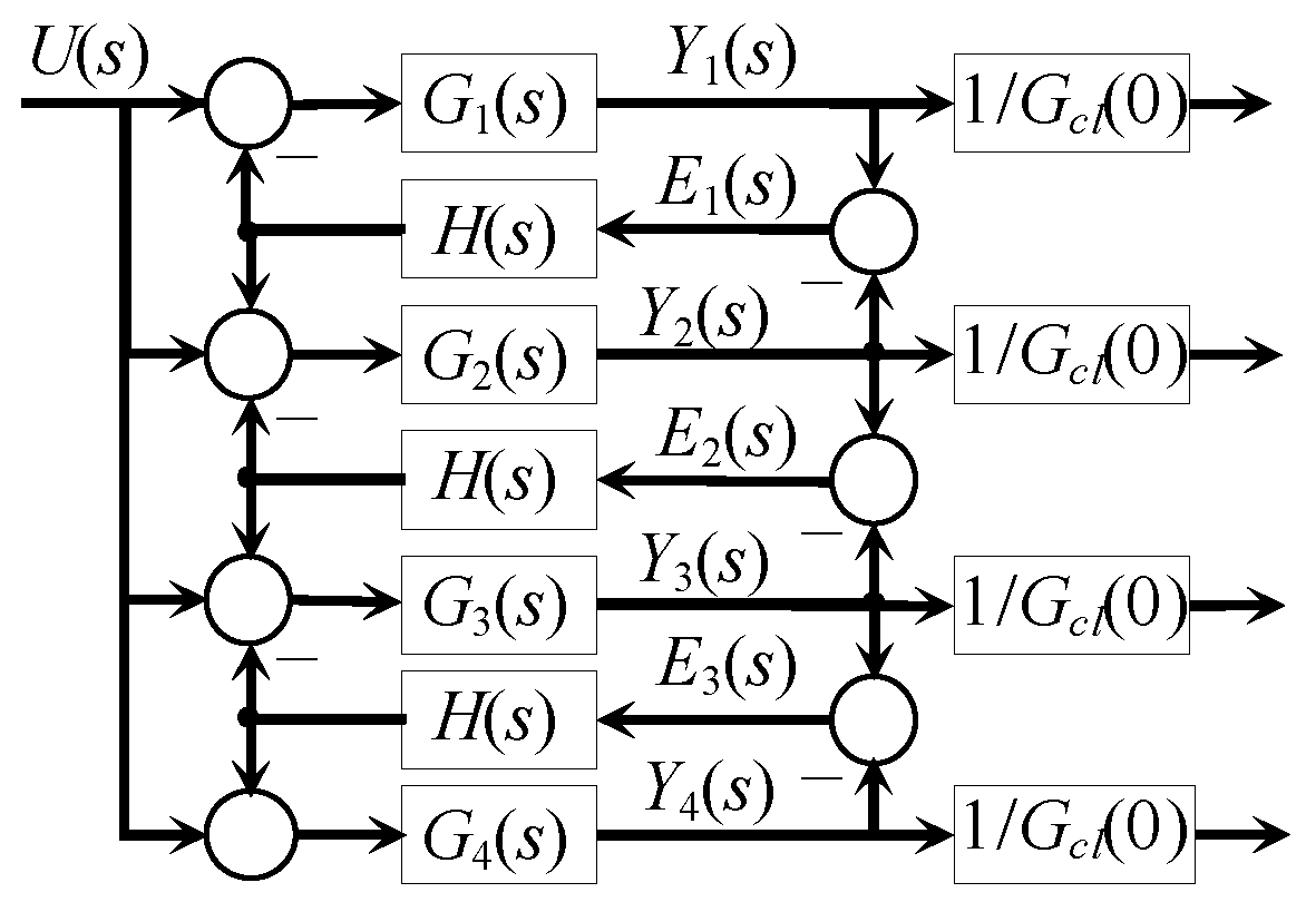
2.3. Synchronised Operation of Multiple Actuators

The problem of synchronising several pitch actuators has recently been treated in [22]. The topic has origins in the theoreticical works, which were first presented in [25,26,27,28,29]. The approach can be considered a particular case of the cross-coupled control method [23,24]. Methods for synchronous control are summarised and reviewed in, e.g., [21].

The case considered in this work includes a number of similar n actuators described using transfer functions G_i(s) = B_i(s)/[sⁿⁱ A_i(s)] with Hurwitz denominators and i = 1…n, whose output responses y_i(t) approach distinct values for a common step input U(s). Hence, the objective is to find a set of (n − 1) identical synchronisers, H(s) = Q(s)/P(s), such that the outputs converge to the same value, i.e.,

$$y_1(t){|}_{t\to \infty }=y_2(t){|}_{t\to \infty }=\dots =y_n(t){|}_{t\to \infty }=u(t){|}_{t\to \infty }$$

(10)

where the denominator P(s) has the minimal order that is required to satisfy (8). The configuration for the synchronisation of four actuators is shown in Figure 2.

The outputs are scaled by the closed-loop stationary gain G_cl(0) in order to satisfy the conditions expressed in (11).

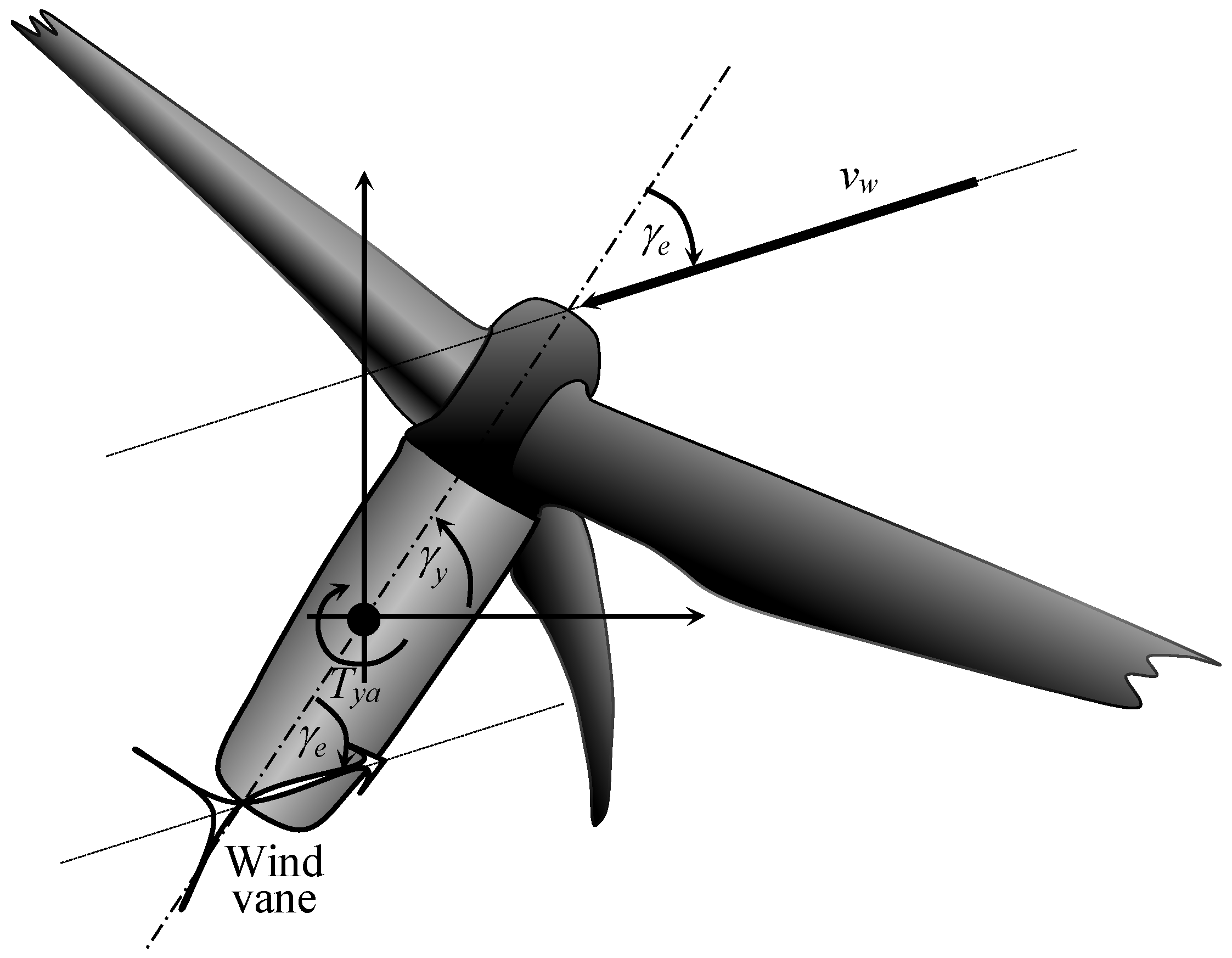
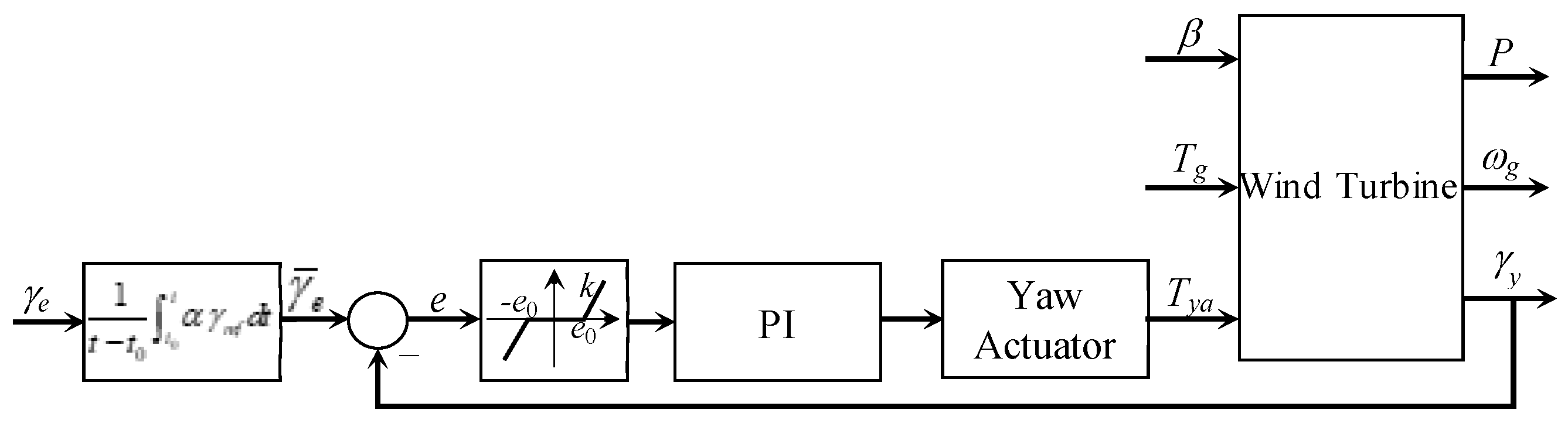
3. Yaw Control of Wind Turbines

In order to align the rotor with the wind direction, the yaw actuators are operated, causing the nacelle to turn around the vertical axis of the tower. This can be carried out if the wind direction is known, which can be obtained by means of a wind vane. The process of aligning the rotor with the wind direction is illustrated in Figure 3.

A controller with a dead zone [40] is commonly utilised to implement a conventional yaw control loop. Due to the dead zone, the controller is only activated when the control error overflows the predetermined threshold given by the dead zone, and its purpose is to return the operation to the region [41]. As the reference to be tracked, a weighted averaged wind direction signal, $\overline{{\gamma }_e}$, is used, which is derived from a wind vane placed at the rear of the nacelle and a low-pass filter. The control system scheme is shown in Figure 4.

The controller is normally implemented as a PI control law, which becomes active when the control error exceeds the dead zone defined in the band [−e₀, e₀] as

$$e_o(t)=\left\{\begin{array}{ll}0\hfill & |e(t)| \le \left|e_0\right|\hfill \\ k e(t)\hfill & |e(t)| > \left|e_0\right|\hfill \end{array}\right.$$

(11)

The measured output is the yaw angle $\gamma$_y (see Figure 3), such that the control error is e =$\overline{{\gamma }_e}-{\gamma }_y$.

The measurement of the wind direction is imprecise and noisy. Therefore, it is essentially inadequate to be used as a setpoint for the control system. Consequently, it is smoothed here by passing it through a moving average filter. However, continuously tracking the reference is unnecessary because the yaw mechanism operates very slowly. Hence, it can be activated only when the misalignment becomes noticeable. That is the duty of the dead zone.

As will be shown later in the practical study, a standard dead zone strongly reduces performance: if it is chosen large to reduce the yaw activity, the tracking is poor, reducing the energy conversion, and if it is small, shattering occurs around the reference. For this reason, an adaptive dead zone is implemented in this work, such that the zone is chosen small when the error is large to ensure that the output variable very closely resembles the reference and then changes to a larger zone to reduce the activity of the yaw mechanism once the output is near the reference.

Moreover, the performance of a standard yaw control system is also improved by replacing the classic PI with the NPI controller. The control law is then

$$u(t) =f_p[e(t)][b r(t)-y(t)]+{\displaystyle {\int }_0^t\{f_i}[e(t)]e(t)+K_a [\overline{u}(t)-u(t)\}dt$$

(12)

where ū(t) is the control signal after the actuator, which is used for the anti-windup mechanism, and f_p and f_i are the nonlinear functions defined by (8) and (9).

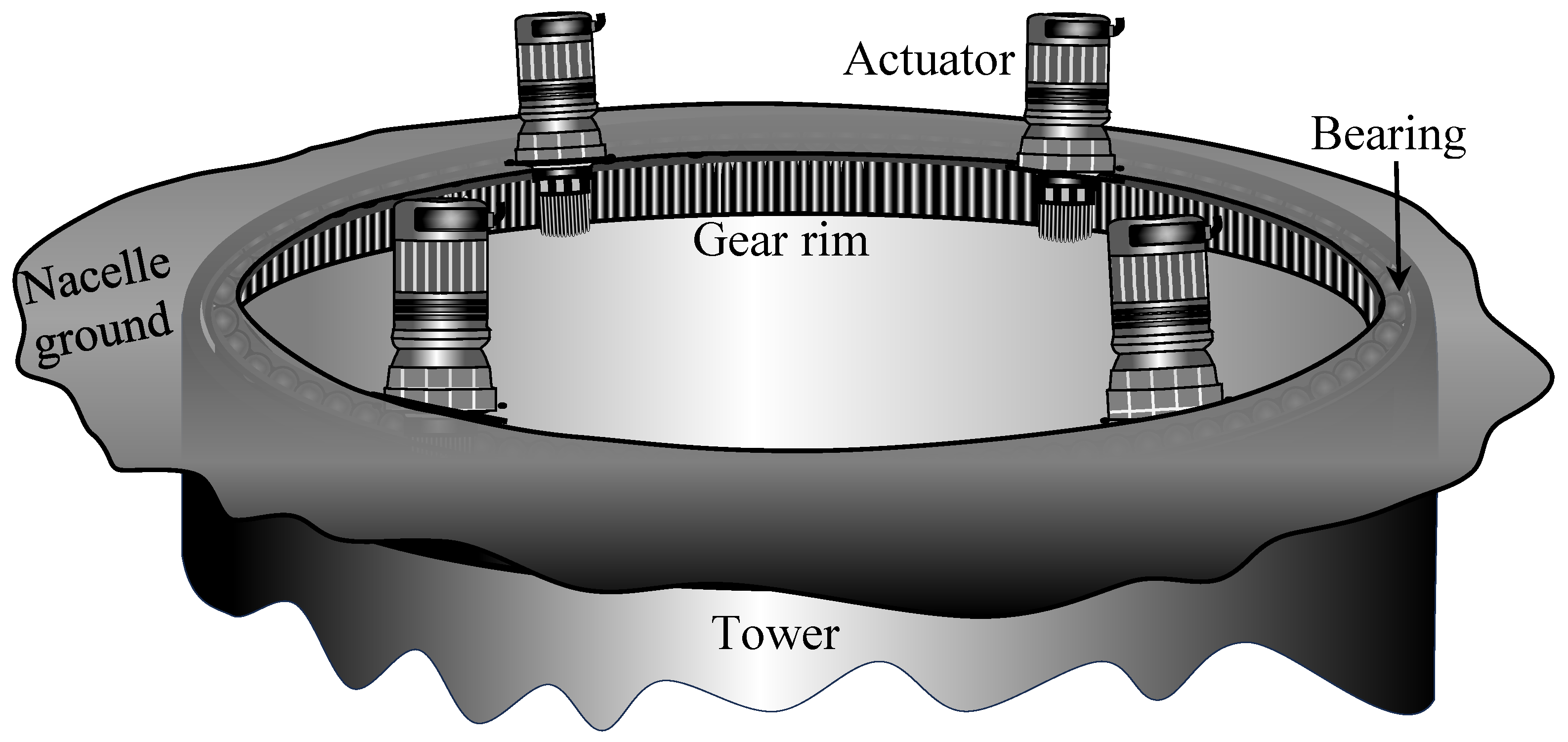
4. Yaw Actuator Control

4.1. Control System for an Individual Actuator

The control of an actuator based on PMSG is described in detail in [22]. The complete control system, which includes two PI current controllers with nonlinear feedforward terms, one PI speed controller with zero compensation, and a derivative feedforward-feedback controller, is shown in Figure 5.

The transfer function for the closed-loop system is then expressed by

$${\mathrm{\Theta }}_m(s)={\displaystyle \frac{ (K_{p\theta }+K_{vff}s)B_s(s)}{s A_s(s)+B_s(s)K_{p\theta }}} {\mathrm{\Theta }}_{mref}(s)-{\displaystyle \frac{B_T(s)}{s A_s(s)+B_s(s)K_{p\theta }}}{{\rm T}}_L(s)$$

(13)

$$\begin{gathered} B_s(s)=b_{m1}{a}_{i2}{K}_{i\omega }, A_s(s)=s(s+a_{m1})(s^2+a_{i1} s+a_{i2})+b_{m1}{a}_{i2}(b K_{p\omega } s+K_{i\omega })\mathrm{and} \\ {B}_T(s)=b_{m1} s (s^2+a_{i1} s+a_{i2}) \end{gathered}$$

(14)

where b_m1 = 1/J_m, a_m1 = B_m/J_m, $a_{i1}=(R_s+K_{pq})/L_q$, and $a_{i2}=K_{iq}/L_q$. The parameters L_d, L_q, R_s, J_m, and B_m are inductances, resistance, the mass moment of inertia, and the viscous friction of the motor, respectively. The gains K_pq, K_vff, K_pw K_iw, K_pq, and K_iq are the parameters of the different controllers. Notice that, in the case of the NP controller, the gain K_pq is variable with the control error.

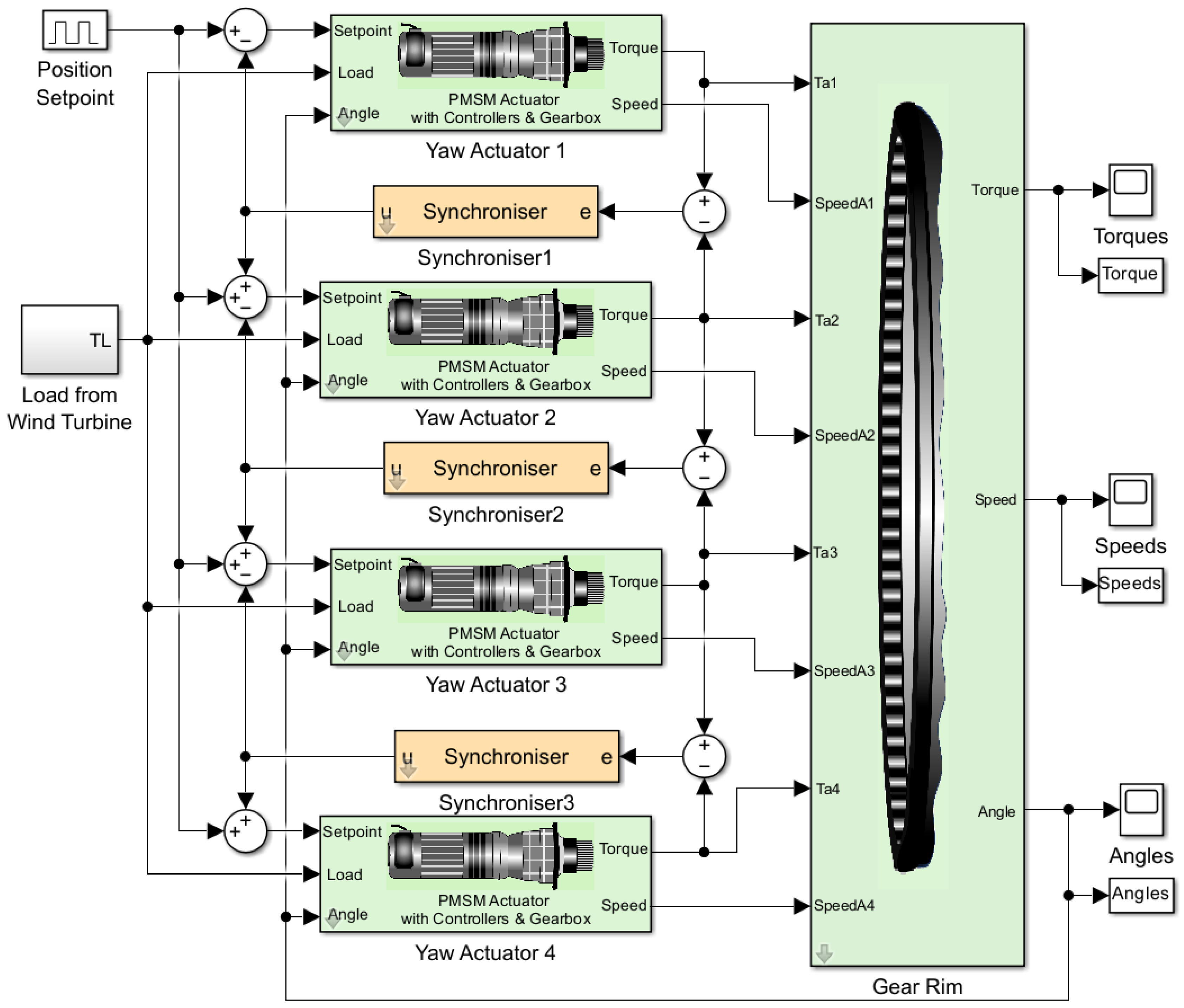
4.2. Synchronised Operation of Multiple Yaw Actuators

Since all actuators are attached to the same gear rim, the interest here is to synchronise the torques. Hence, the synchronisation for n actuators is carried out by means of (n − 1) identical NPI controllers according to (8), (9), and (12) but with a different parametrisation, namely

$$f_{ps}(e)=K_{0ps}+K_{1ps}[1-\mathrm{sech}(K_{2ps}e)]\mathrm{and}$$

(15)

$$f_{is}(e)=K_{0is}+K_{1is}[1-\mathrm{sech}(K_{2is}e)]$$

(16)

The control system configuration is portrayed in Figure 6.

5. Application Study

5.1. Parametrisation of the Reference Wind Turbine

The wind turbine objective for the numerical study is the three-bladed 5-MW machine from NREL [42], whose maximum yaw load moment is estimated to be about T_g = 7833.7 kNm. The rotor has a diameter of 126 m and a hub height of 90 m. The tower top diameter is 3.87 m. The rated yaw speed is w_gn = 0.05 rpm.

Notice that the wind turbine has a high number of parameters and specifications; see [42] for a list of them.

5.2. Parametrisation of the Yaw Actuator Model

The specifications for the actuator are a yaw speed of w_g = 0.05 rpm, and the tower top diameter d_t = 3.87 m, which is considered the gear rim diameter. The pinion diameter is d_p = 0.16 m.

In comparison to the torque of commercial yaw actuators, the maximal load moment is highly exceeding such actuator torques. Therefore, it is necessary to implement several joint-working yaw actuators in order to manage the load torque. The link between the motor torque and the load torque is denoted as

$$T_{\gamma }=n_a{n}_m{n}_x{T}_m$$

(17)

The parameter n_a represents the number of necessary actuators, n_m symbolises the gear rim ratio, and n_x is the ratio of the gearbox. The gear rim ratio is obtained from n_m = d_t/d_p = 3.87/0.16 = 24.2. The gearbox ratio, n_x, can be computed as w_m/(n_mw_g), where w_g and w_m are the yaw speed and the as motor speed, respectively. Under these definitions, (9) becomes

$$T_{\gamma }={\displaystyle \frac{n_a{n}_m{\omega }_m}{n_m{\omega }_{\gamma }}}{T}_m={\displaystyle \frac{n_a{\omega }_m}{{\omega }_{\gamma }}}{T}_m$$

(18)

A PMSM with six pole pairs, a torque of 102 Nm, and 960 rpm (100.531 rad/s) is selected for the yaw actuation. Hence, it follows that

$$n_x={\displaystyle \frac{{\omega }_m}{n_m{\omega }_{\gamma }}}={\displaystyle \frac{960}{24.2 0.05}}=793.4$$

(19)

The required number of yaw actuators is

$$n_a={\displaystyle \frac{T_{\gamma }}{n_m{n}_x{T}_m}}={\displaystyle \frac{7833700}{24.2 793.4 102}}\simeq 4$$

(20)

The attachment of four actuators to the gear rim is schematised in Figure 7.

In addition, the nominal values for line-to-line voltage are 230 V (v_sd = 96.3 V and v_sq = 208.9 V) and a current of 230.52 A (i_sd = 163 A and i_sq = 163 A). Moreover, the torque difference in the stationary state is defined as DT = T_e − T_g/(n_a n_m n_x) = 0.1. The steady-state equations in matrix form for the model are expressed as

$$\left[\begin{array}{c}{L}_d\\ R_s\\ {\lambda }_f\\ B_m\end{array}\right]={\left[\begin{array}{cccc}-p{\omega }_m& i_{sd}& 0& 0\\ p{\omega }_m{i}_{sd}& i_{sq}& p\omega & 0\\ 0& 0& 1.5p{i}_{sq}& 0\\ 0& 0& 0& {\omega }_m\end{array}\right]}^{-1}\left[\begin{array}{c}{v}_{sd}\\ v_{sq}\\ T_m\\ \Delta T\end{array}\right]$$

(21)

By solving (13) for p = 6, the physical parameters are L_d = L_q = 0.359343 × 10⁻³ H, R_s = 0.8045 Ω, λ_f = 0.07072 Wb, and B_m = 0.0147 Nm s/rad. The second moment of inertia is estimated by J_m = 1.6134 kg m², which completes the actuator parametrisation. The parameters for the other three actuators are obtained by random parameter variation inside a band of 10% of the first one. All parameters are summarised in

Table 1. Actuator parameters.

Parameters	Actuator 1	Actuator 2	Actuator 3	Actuator 4
Jm [kg m2]	1.6134	1.5327	1.6457	1.6505
Bm [N m/(rad/s)]	0.0147	0.018919	0.0075661	0.009241
Ld [H]	0.00035934	0.00034138	0.00053901	0.00048511
Lq [H]	0.00035934	0.00034138	0.00053901	0.00048511
Rs [Ω]	0.80455	0.76432	1.2068	1.0861
lf [Wb]	0.07072	0.068217	0.076378	0.076095
p	6	6	6	6

.

5.3. Control Systems and Controller Parametrisation

5.3.1. Control Loops and Controller Parameters for the Yaw System

The NPI controller is compared with a standard PI controller. Hence, controller parameters for both are obtained via the simulation-based numerical minimisation of the ITSE objective function (integral time-weighted squared error, see (22)) by using the active-set method under stability constraints, i.e., Hurwitz closed-loop poles. All parameters are summarised in

Table 2. Parameters for the yaw controllers.

Parameters	Proportional Gain	Integral Gain	Actuator 3	Reference Weight
PI	Kpy = 7.372	Kiy = 3.443	Kay = 5	b = 1
NPI	K0py = 4.4173 K1py = 8.6107 K2py = 0.0143	K0iy = 4.4173 K1iy = 8.6107 K2iy = 0.0143	Kay = 5	b = 1

.

5.3.2. Control Loops and Controller Parameters for the Yaw Actuators

As mentioned before, the design of the synchronisers requires the models of the considered plants, in this case, the actuators, which in turn have three levels of cascade control (current, speed, and position control). Thus, the controller parameters of all actuators are needed to design the synchronisers. They are designed individually by using the same procedure as mentioned in the previous section. The simulation results of the separately and decoupled from gear rim controlled actuators are portrayed in Figure 8 for a P position controller and Figure 9 for an NP position controller. The controller parameters are summarised in

Table 3. Controller parameters of actuators.

Parameters		Actuator 1	Actuator 2	Actuator 3	Actuator 4
Current controllers		Kpd = 0.0870 Kid = 0.1710 Kpq = 1.0489 Kiq = 2.5310	Kpd = 0.0870 Kid = 0.1710 Kpq = 1.0489 Kiq = 2.5310	Kpd = 0.0870 Kid = 0.1710 Kpq = 1.0489 Kiq = 2.5310	Kpd = 0.0870 Kid = 0.1710 Kpq = 1.0489 Kiq = 2.5310
Speed controllers		Kpt = 4.1952 Kit = 0.0290	Kpt = 1.5646 Kit = 0.0215	Kpt = 3.5038 Kit = 0.0192	Kpt = 5.7635 Kit = 0.0294
Position controllers	FF	Kvff = 20.6395	Kvff = 20.6395	Kvff = 22.2367	Kvff = 26.2889
	P	Kpp = 20.1020	Kpp = 20.2919	Kpp = 20.8031	Kpp = 20.3189
	NP	Kpp1 = 15.4355 Kpp2 = 2.3869 Kpp3 = 1.0000	Kpp1 = 1.2978 Kpp2 = 16.4546 Kpp3 = 1.0000	Kpp1 = 12.6032 Kpp2 = 5.0307 Kpp3 = 1.0000	Kpp1 = 9.8339 Kpp2 = 8.0440 Kpp3 = 1.0000

.

The NP position control demonstrates superior performance compared to the P controllers, particularly in terms of output angles. Values of performance indices J_e (integral time-weighted squared error, ITSE, see (17)) are summarised in

Table 4. Values of the performance index for all actuators without synchronisation.

	P Position Controller				NP Position Controller
	Actuator 1	Actuator 2	Actuator 3	Actuator 4	Actuator 1	Actuator 2	Actuator 3	Actuator 4
Je	685.5	543.5	743.4	564.5	211.4	480.6	598.5	559.3

.

5.4. Setup for the Simulation Environment

The wind turbine simulations take place in OpenFAST V4.1.0 from NREL (formerly known as FAST [43]). The wind speed is chosen to be stepwise with 5% turbulence in the x- and y-directions changing between 12 and 22 m/s (see Figure 10).

5.5. Description of the Simulation Experiments

The simulation experiments are divided into two groups. The first group is dedicated to the yaw control. Simulations are carried out for different dead zones and for the classic PI, as well as the NPI controllers. For the comparison, three objective functions are evaluated, namely

$$J_e={\displaystyle \frac{1}{t_f-t_i}}{\displaystyle {\int }_{t_i}^{t_f}t {[e_{\gamma }(t)/e_{\gamma max}]}^{2}dt}, J_u={\displaystyle \frac{1}{t_f-t_i}}{\displaystyle {\int }_{t_i}^{t_f}t {[u(t)/u_{max}]}^{2}dt}, \mathrm{and} E={\displaystyle \frac{1}{3600}}{\displaystyle {\int }_{t_i}^{t_f}t P_e(t) dt}$$

(22)

J_e and J_u are the averaged integral of time-weighted squared control error (ITSE) and of the squared control signal (ITSU), respectively. The last one, E, is the average energy converted, expressed in kWh. While in the first two functions, smaller numbers indicate better performance, in the third one, the improvement in performance is characterised by an increase in the value of converted energy.

The second group of experiments is devoted to the synchronisation of yaw actuators, also considering PI, as well as NPI controllers as synchronisers. The objective functions are evaluated in this case considering the differences between the output torques of the actuators.

6. Simulation Results and Analysis

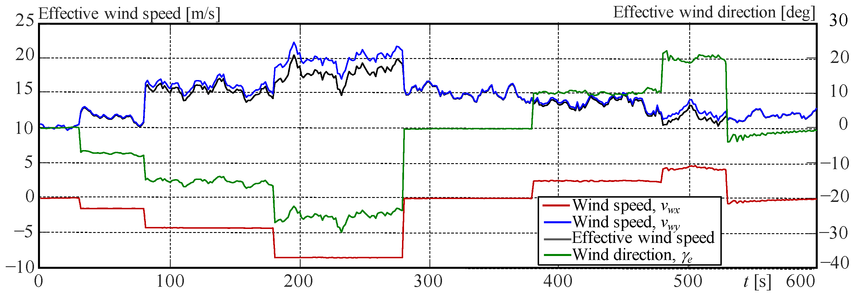
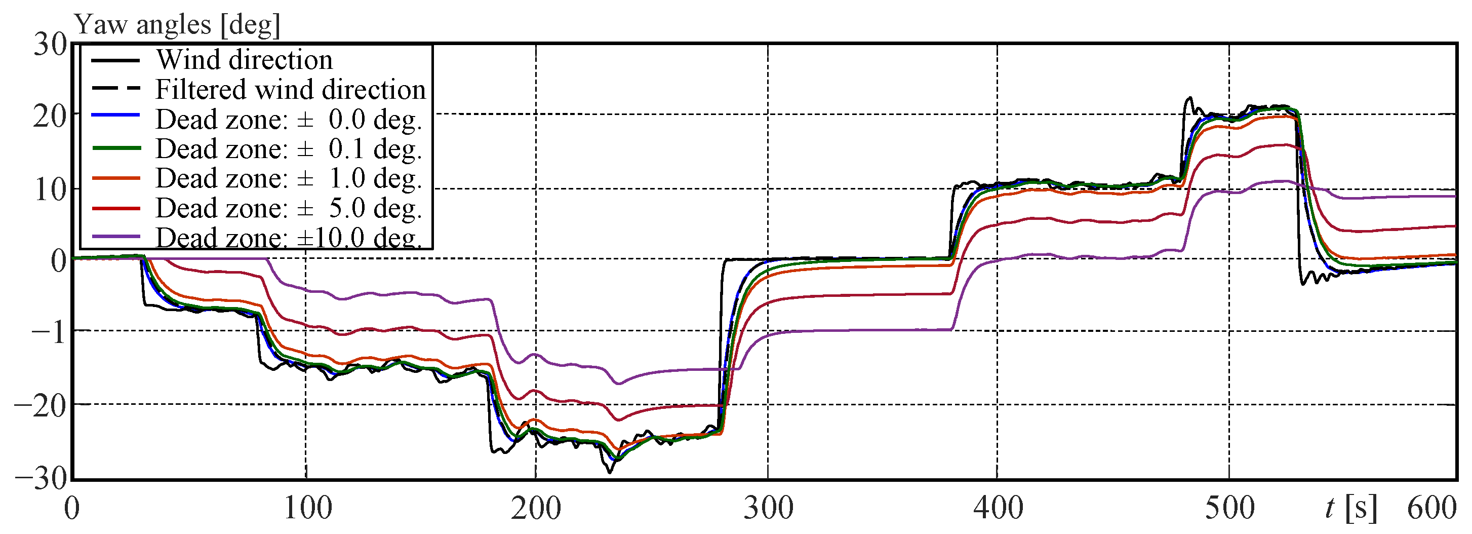
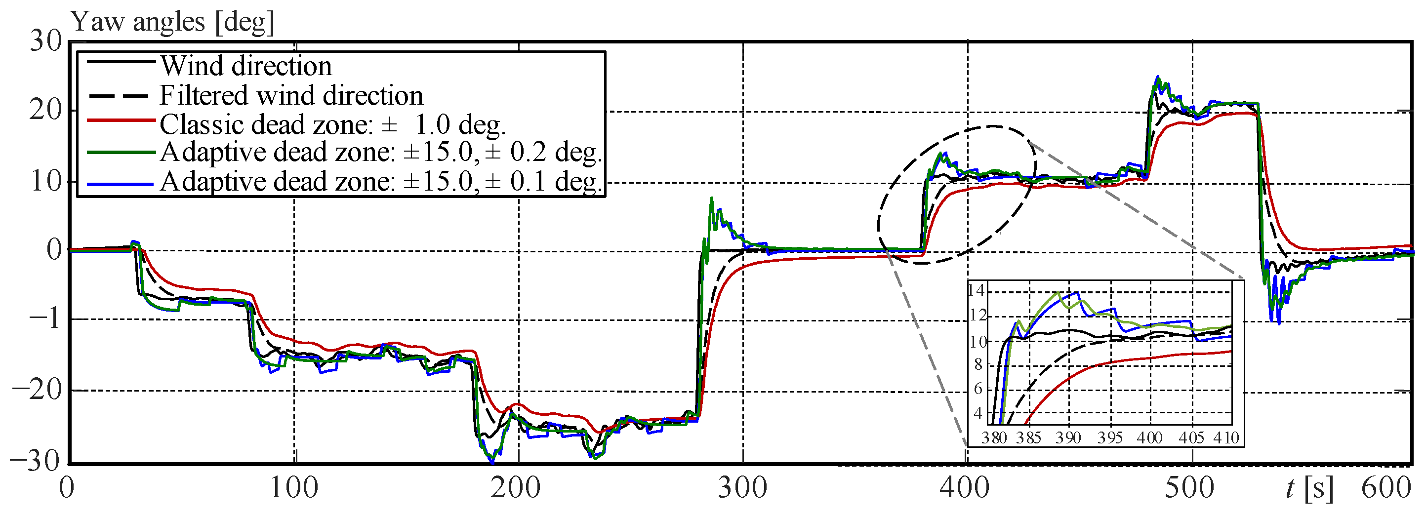
6.1. Simulation Results for the Yaw Control Experiment

First, the performances of PI and NPI controllers without a dead zone are compared. As a reference signal to be tracked, the moving-averaged filtered wind direction is used. The results are shown in Figure 11.

It is possible to observe that the NPI shows a practically perfect tracking performance while the PI controller is a bit inferior. The quantitative comparison indicates J_e = 0.3566 for the PI controller and J_e = 0.0071 for the NPI. The energy conversion E is also slightly better for the NPI (262.8 against 262.0), and both have practically the same control activity J_u = 68.594.

The second experiment consists of testing the yaw control system for different dead zones. Yaw mechanisms are normally not designed for continuous operation. The necessary inactivity is implemented by a dead zone, where inactivity time is given by the width of the dead zone. During the inactivity, the yaw angle can drift away from the reference. Therefore, the performance of the wind turbine will deteriorate in the time that the yaw mechanism is inactive. Thus, the aim of this test is to find a compromise between reduced deteriorated performance and reduced yaw activity. This is studied by testing different dead zones. The simulation results are presented in Figure 12.

The curves show the tracked yaw angles regarding the reference (dashed curve). The control errors are given by the distance between the curve corresponding to the considered dead zone and the reference. It is clear that the control errors increase with the increasing width of the dead zone.

The quantitative analysis summarised in

Table 5. Values of performance indices for PI and NPI controllers with different dead zones.

Dead Zone	PI			NPI
	Je	Ju	E	Je	Ju	E
0 deg	0.3566	68.5939	262.0	0.0071	68.5942	262.8
±0.1 deg	0.4182	69.1778	262.0	0.0269	68.9010	263.0
±1.0 deg	1.2507	68.1147	261.4	0.4072	65.6015	262.8
±5.0 deg	17.6656	62.3505	256.1	6.8705	78.0999	258.2
±10.0 deg	100.9248	73.2117	242.0	26.3100	77.2117	252.7
Adaptive: (±0.2, ±15.0) deg	0.4775	69.1624	261.9	0.0380	69.4918	261.9
Adaptive: (±0.1, ±15.0) deg	0.4009	69.2013	262.0	0.0290	68.8906	262.0

indicates that the PI controller with a dead zone of ±5.0 deg yields the minimum actuator activity (J_u = 62.3505), but, on the other hand, the energy conversion is reduced (E = 256.1) and the tracking performance is poor (J_e = 17.6656). Notice that the NPI with a dead zone ±1.0 deg has a comparable actuator activity (J_u = 65.6015) but achieves good tracking performance (J_e = 1.2507) and energy conversion (E = 262.8).

In the last experiment, the yaw control system is implemented with the adaptive dead zone, considering two cases. In the first one, the dead zone width changes from ±15.0 to ±0.2 degrees, and in the last one, the change is between ±15.0 and ±0.1 degrees. The results are depicted in Figure 13 compared with the best case of fixed dead zones.

The idea of the adaptive dead zone is to improve the tracking performance without a significant increment in actuator activity.

Finally, all results regarding the quantitative study are summarised in Table 5.

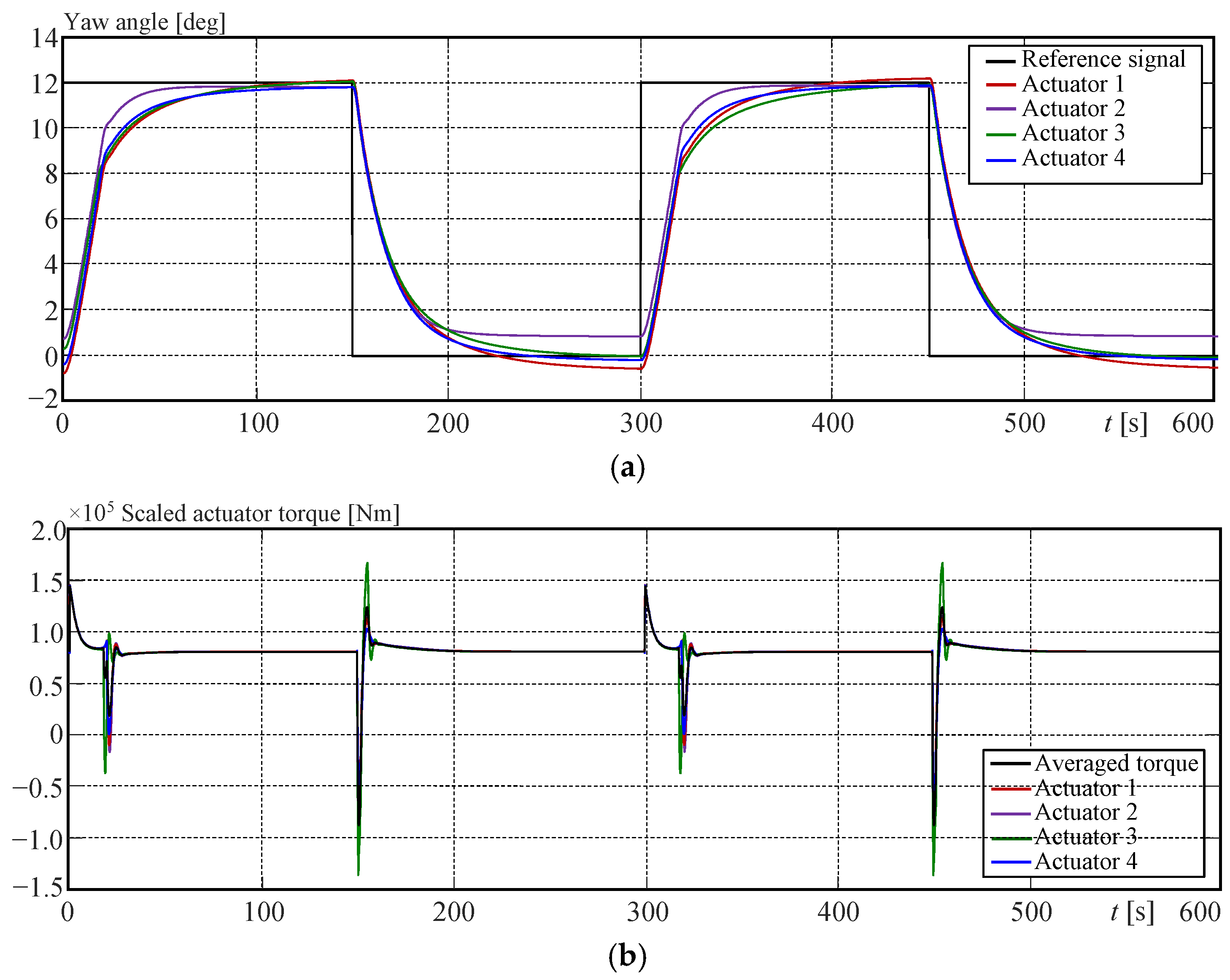
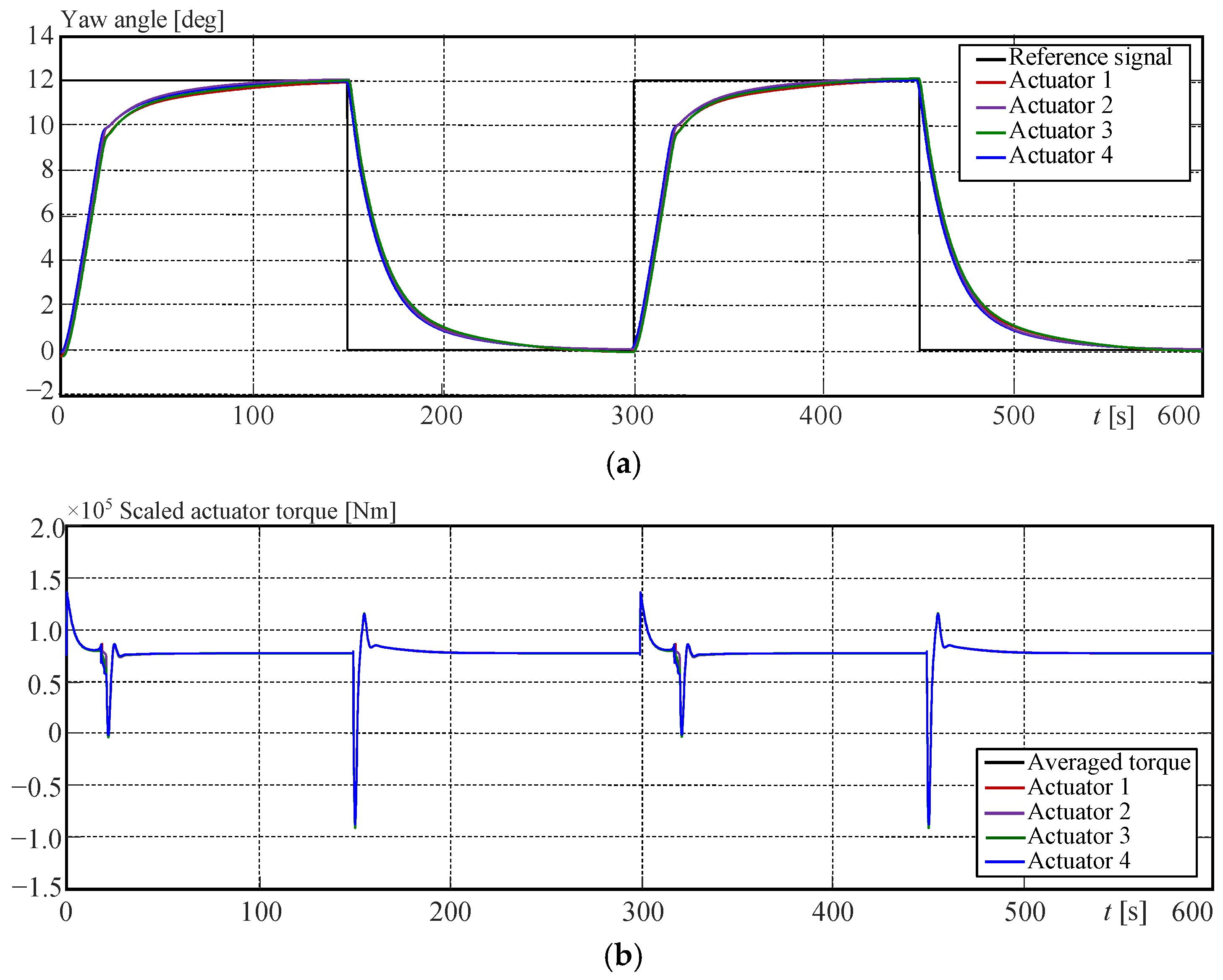
6.2. Simulation Results for the Yaw Actuator Control Experiment

The yaw actuator control was first implemented by using PI control for the current and speed controllers and a P controller for the position, following the classic approach [44]. The synchronisers were also implemented as PI controllers. Later, all position controllers and the synchronisers were changed to NP and NPI control laws.

Since all actuators are attached to the same gear rim, balanced torque distribution is an essential aspect, but the angles are also synchronised because of mechanical constraints.

The synchronised control with PI controllers is shown in Figure 14, and with NPI controllers in Figure 15.

The results of the computed performance indices are expressed in

Table 6. Values of the performance index for all actuators with synchronisation.

	PI Synchronisers				NPI Synchronisers
	Actuator 1	Actuator 2	Actuator 3	Actuator 4	Actuator 1	Actuator 2	Actuator 3	Actuator 4
Je	206.03	432.01	151.09	154.91	30.20	47.85	45.23	95.73

.

When Table 5 and Table 6 are compared, it is clear that the synchronisation provides an important improvement regarding the non-synchronised approach. Moreover, NPI synchronisers also present an improved performance with respect to the PI controllers.

7. Conclusions

This study has been devoted to investigating the problem of tracking the wind direction of large wind energy converters, which is known as yaw control. Two aspects were considered. The first one was the yaw control problem itself, considering dead zones in order to reduce the actuator activity. The second aspect concerns the necessity of several actuators attached to the same gear rim to move the rotor and nacelle, which makes the synchronisation of these actuators important.

Yaw control is normally implemented using PI controllers. The synchronisation of yaw actuators is actually a new topic, but synchronisers can also be implemented with PI control laws. In order to improve the control performance regarding the tracking of the wind direction, the use of nonlinear P and PI controllers was explored.

The experiments were conducted on the NREL 5 MW reference wind turbine, which was implemented in OpenFAST. For the control system, MATLAB^®/Simulink (R2024a) were utilised. The simulation results were evaluated qualitatively according to the portrayed curves and quantitatively by using performance indices.

In general, NPI controllers showed the best performance in all cases. Moreover, the yaw control with an adaptive dead zone offers a better balance between actuator activity and power reduction due to misalignment, which is an advantage in the farm control application. The most important inconvenience in the case of yaw control is the inaccurate measurement or estimation of the wind direction. Hence, this aspect will be deeply studied in future work.

Concerning the actuator synchronisation problem, there are several possible research lines. The case of many actuators is one of the most important to be studied. For instance, about 16 yaw actuators are necessary for a 12 MW wind turbine [45], whose synchronisation can be very challenging.

References

1. Liu, Y.; Liu, S.; Zhang, L.; Cao, F.; Wang, L. Optimization of the yaw control error of wind turbines. Front. Energy Res. 2021, 9, 626681. [Google Scholar] [CrossRef]
2. Bastankhaha, M.; Porté-Agelb, F. Wind farm power optimization via yaw angle control: A wind tunnel study. J. Renew. Sustain. Energy 2019, 11, 023301. [Google Scholar] [CrossRef]
3. Howland, M.F.; Lele, S.K.; Dabiria, J.O. Wind farm power optimization through wake steering. Proc. Natl. Acad. Sci. USA 2019, 116, 14495–14500. [Google Scholar] [CrossRef] [PubMed]
4. Knudsen, T.; Bak, T.; Svenstrup, M. Survey of wind farm control—Power and fatigue optimization. Wind Energy 2015, 18, 1333–1351. [Google Scholar] [CrossRef]
5. Yang, J.; Fang, L.; Song, D.; Su, M.; Yang, X.; Huang, L.; Joo, Y.H. Review of control strategy of large horizontal-axis wind turbines yaw system. Wind Energy 2021, 24, 97–115. [Google Scholar] [CrossRef]
6. Song, D.; Yang, J.; Fan, X.; Liu, Y.; Liu, A.; Chen, G.; Joo, Y.H. Maximum power extraction for wind turbines through a novel yaw control solution using predicted wind directions. Energy Convers. Manag. 2018, 157, 587–599. [Google Scholar] [CrossRef]
7. Chen, W.; Liu, H.; Lin, Y.; Li, W.; Sun, Y.; Zhang, D. LSTM-NN yaw control of wind turbines based on upstreamWind information. Energies 2020, 13, 1482. [Google Scholar] [CrossRef]
8. Fleming, P.A.; Scholbrock, A.K.; Jehu, A.; Davoust, S.; Osler, E.; Wright, A.D.; Clifton, A. Field-test results using a nacelle-mounted lidar for improving wind turbine power capture by reducing yaw misalignment. J. Phys. Conf. Ser. 2014, 524, 012002. [Google Scholar] [CrossRef]
9. Yang, M.; Fan, S.; Lee, W.J. Probabilistic short-term wind power forecast using componential sparse Bayesian learning. IEEE Trans. Ind. Appl. 2013, 49, 2783–2792. [Google Scholar] [CrossRef]
10. Kavousi-Fard, A.; Khosravi, A.; Nahavandi, S. A new fuzzy-based combined prediction interval for wind power forecasting. IEEE Trans. Power Syst. 2016, 31, 18–26. [Google Scholar] [CrossRef]
11. Ouyang, T.; Kusiak, A.; He, Y. Predictive model of yaw error in a wind turbine. Energy 2017, 123, 119–130. [Google Scholar] [CrossRef]
12. Karakasis, N.; Mesemanolis, A.; Nalmpantis, T.; Mademlis, C. Active yaw control in a horizontal axis wind system without requiring wind direction measurement. IET Renew. Power Gener. 2016, 10, 1441–1449. [Google Scholar] [CrossRef]
13. Guo, F.; Jiang, W.; Shao, H.; Du, Y.; She, J. Research on the wind turbine yaw system based on PLC. In Proceedings of the 29th Chinese Control and Decision Conference (CCDC), Chongqing, China, 28–30 May 2017; pp. 5164–5168. [Google Scholar]
14. Farret, F.A.; Pfitscher, L.L.; Bernardon, D.P. Sensorless active yaw control for wind turbines. In Proceedings of the 27th Annual Conference of the IEEE Industrial Electronics Society, Denver, CO, USA, 29 November–2 December 2001; pp. 1370–1375. [Google Scholar] [CrossRef]
15. Wu, X.; Liu, Y.; Teng, W. Modified hill climbing method for active yaw control in wind turbine. In Proceedings of the 31st Chinese Control Conference, Hefei, China, 25–27 July 2012; pp. 6677–6680. [Google Scholar]
16. Ekelund, T. Yaw control for reduction of structural dynamic loads in wind turbines. J. Wind. Eng. Ind. Aerodyn. 2000, 85, 241–262. [Google Scholar] [CrossRef]
17. Hure, N.; Turnar, R.; Vasak, M.; Bencic, G. Optimal wind turbine yaw control supported with very short-term wind predictions. In Proceedings of the IEEE International Conference on Industrial Technology (ICIT), Seville, Spain, 17–19 March 2015; pp. 385–391. [Google Scholar] [CrossRef]
18. Kragh, K.A.; Hansen, M.H. Load alleviation of wind turbines by yaw misalignment. Wind Energy 2014, 17, 971–982. [Google Scholar] [CrossRef]
19. Hu, S.; Ren, X.; Zhao, W. Synchronous control of multi-motor driving servo systems. In Lecture Notes in Electrical Engineering; Jia, Y., Du, J., Zhang, W., Eds.; Springer: Singapore, 2017; Volume 459, pp. 611–620. [Google Scholar] [CrossRef]
20. Li, M.; Meng, X. Analysis and design of system for multi-motor synchronous control. In Advances in Computer Science, Environment, Ecoinformatics, and Education; Lin, S., Huang, X., Eds.; Springer: Berlin/Heidelberg, Germany, 2011; Volume 217, pp. 268–273. [Google Scholar] [CrossRef]
21. Niu, F.; Sun, K.; Huang, S.; Hu, Y.; Liang, D. A review on multimotor synchronous control methods. IEEE Trans. Transp. Electrif. 2023, 9, 22–33. [Google Scholar] [CrossRef]
22. Gambier, A. Synchronised control of multiple actuators of wind turbines. Actuators 2025, 14, 264. [Google Scholar] [CrossRef]
23. Koren, Y. Cross-coupled biaxial computer control for manufacturing systems. J. Dyn. Syst. Meas. Control 1980, 102, 265–271. [Google Scholar] [CrossRef]
24. Zhao, D.; Li, C.; Ren, J. Speed synchronization of multiple induction motors with adjacent cross coupling control. In Proceedings of the 48h IEEE Conference on Decision and Control (CDC), Shanghai, China, 15–18 December 2009; pp. 6805–6810. [Google Scholar] [CrossRef]
25. Unbehauen, H.; Vakilzadeh, I. Synchronization of n non-identical simple-integral plants. Int. J. Control 1989, 50, 543–574. [Google Scholar] [CrossRef]
26. Vakilzadeh, I.; Mansour, M. Synchronization of ‘n’ integral-plus-times constant plants with non-identical gain and time constants. Control Theory Adv. Technol. 1989, 5, 569–585. [Google Scholar] [CrossRef]
27. Vakilzadeh, I.; Mansour, M. Synchronization of ‘n” integral-plus-double time constant plants with non-identical gain and time constants. J. FrankIm. Inst. 1990, 327, 579–593. [Google Scholar] [CrossRef]
28. Unbehauen, H.; Vakilzadeh, I. Synchronization of ‘n’ decentralized non-identical plants with integral behavior and two complex poles. Control Theory Adv. Technol. 1994, 10, 385–402. [Google Scholar]
29. Vakilzadeh, I.; Unbehauen, H. Four rendezvous problems for n non-identical simple-integral plants. Int. J. Syst. Sci. 1993, 24, 1455–1472. [Google Scholar] [CrossRef]
30. Shahruz, S.M.; Schwartz, A.L. Design of optimal nonlinear PI compensators. In Proceedings of the 32nd IEEE Conference on Decision and Control, San Antonio, TX, USA, 15–17 December 1993; pp. 3564–3565. [Google Scholar]
31. Xu, Y.; Hollerbach, J.M.; Ma, D. A nonlinear PD controller for force and contact transient control. IEEE Control Syst. Mag. 1995, 15, 15–21. [Google Scholar]
32. Gambier, A.; Nazaruddin, Y. Collective pitch control with active tower damping of a wind turbine by using a nonlinear PID approach. IFAC 2018, 51, 238–243. [Google Scholar] [CrossRef]
33. Åström, K.J.; Hagglund, T. Advanced PID control, ISA-The Instrumentation, Systems, and Automation Society; Research Tringle Park: Durham, NC, USA, 2006. [Google Scholar]
34. Visioli, A. Practical PID Control; Springer: London, UK, 2006. [Google Scholar]
35. Seraji, H. A new class of nonlinear PID controllers with Robotic Applications. J. Robot. Syst. 1998, 15, 161–181. [Google Scholar] [CrossRef]
36. Su, Y.X.; Sun, D.; Duan, B.Y. Design of an enhanced nonlinear PID controller. Mechatronics 2005, 15, 1005–1024. [Google Scholar] [CrossRef]
37. Taylor, J.H.; Strobel, K.L. Nonlinear compensator synthesis via sinusoidal-input describing functions. In Proceedings of the 1985 American Control Conference, Boston, MA, USA, 19–21 June 1985; pp. 1242–1247. [Google Scholar]
38. Isayed, B.M.; Hawwa, M.A. A nonlinear PID control scheme for hard disk drive servosystems. In Proceedings of the 15th Mediterranean Conference on Control and Automation, Athens, Grecce, 27–29 June 2007; pp. 1–6. [Google Scholar] [CrossRef]
39. Junoh, S.C.K.; Salim, S.N.S.; Abdullah, L.; Anang, N.A.; Chiew, T.H.; Retas, Z. Nonlinear PID triple hyperbolic controller. Int. J. Mech. Mechatron. Eng. Des. XY Table Ball-Screw Drive Syst. 2017, 17, 1–10. [Google Scholar]
40. Slotine, J.-J.; Li, W. Applied Nonlinear Control; Prentice Hall, Englewood Cliffs: New Jersey, NJ, USA, 1991. [Google Scholar]
41. Burton, T.; Jenkins, N.; Sharpe, D.; Bossanyi, E. Wind Energy Handbook Edition, 2nd ed.; John Wiley and Sons: Chichester, UK, 2011. [Google Scholar]
42. Jonkman, J.; Butterfield, S.; Musial, W.; Scot, G. Definition of a 5-MW Reference Wind Turbine for Offshore System Development. Technical Report; NREL: Golden, CO, USA, 2009. [Google Scholar]
43. Jonkman, J.M.; Buhl Jr, L.M. FAST User’s Guide; Research report, NREL; Battelle: Golden, CO, USA, 2005. [Google Scholar]
44. Wang, L.; Chai, S.; Yoo, D.; Gan, L.; Ng, K. PID and Predictive Control of Electrical Drives and Power Converters Using MATLAB®/Simulink®; John Wiley & Sons: Singapore, 2015. [Google Scholar]
45. Bonfiglioli. Wind Solutions: Product Range. Product Description; Bonfiglioli Riduttori S.p.A.: Carpiano, Italy, 2020. [Google Scholar]
Figure 1. (a) Basic nonlinear function g(e) with two different values of K2. (b) Scaled nonlinear function f(e).
Machines 13 00644 g001
Figure 2. Synchronisation of four actuators.
Machines 13 00644 g002
Figure 3. Yaw misalignment of a wind turbine.
Machines 13 00644 g003
Figure 4. Scheme of a yaw control system with dead zone.
Machines 13 00644 g004
Figure 5. Block diagram of the actuator and its control system [22].
Machines 13 00644 g005
Figure 6. Block diagram of the synchronised actuator control system.
Machines 13 00644 g006
Figure 7. Simplified scheme of four actuators attached to the gear rim.
Machines 13 00644 g007
Figure 8. Angles (a) and torques (b) of each actuator separately with P position control.
Machines 13 00644 g008
Figure 9. Angles (a) and torques (b) of each actuator separately with NP position control.
Machines 13 00644 g009
Figure 10. Wind profile used in the simulation experiments.
Machines 13 00644 g010
Figure 11. Controlled yaw angles using PI, as well as NPI controllers.
Machines 13 00644 g011
Figure 12. NPI control results for different dead zones.
Machines 13 00644 g012
Figure 13. NPI control with adaptive dead zones.
Machines 13 00644 g013
Figure 14. Angles (a) and torques (b) for the synchronised actuator control with PI controllers.
Machines 13 00644 g014
Figure 15. Angles (a) and torques (b) with NPI synchronisers.
Machines 13 00644 g015