Explainable Data Mining Framework of Identifying Root Causes of Rocket Engine Anomalies Based on Knowledge and Physics-Informed Feature Selection

Abstract

Liquid rocket engines occasionally experience abnormal phenomena with unclear mechanisms, causing difficulty in design improvements. To address the above issue, a data mining method that combines ante hoc explainability, post hoc explainability, and prediction accuracy is proposed. For ante hoc explainability, a feature selection method driven by data, models, and domain knowledge is established. Global sensitivity analysis of a physical model combined with expert knowledge and data correlation is utilized to establish the correlations between different types of parameters. Then a two-stage optimization approach is proposed to obtain the best feature subset and train the prediction model. For the post hoc explainability, the partial dependence plot (PDP) and SHapley Additive exPlanations (SHAP) analysis are used to discover complex patterns between input features and the dependent variable. The effectiveness of the hybrid feature selection method and its applicability under different noise combinations are validated using synthesized data from a high-fidelity simulation model of a pressurization system. Then the analysis of the causes of a large vibration phenomenon in an active engine shows that the prediction model has good accuracy, and the feature selection results have a clear mechanism and align with domain knowledge, providing both accuracy and interpretability. The proposed method shows significant potential for data mining in complex aerospace products.

1. Introduction

The liquid rocket engine is the most crucial component of a rocket propulsion system and directly determines flight performance. Therefore, significant effort has been put into product warranty during manufacture, testing, and installation processes. However, abnormal phenomena still occur throughout the engine’s life cycle with mechanisms that are not fully understood. Some of these phenomena are due to complex mechanisms, and there is currently no mature simulation method to directly analyze them. Other phenomena are sensitive to manufacturing processes and unpredictable factors such as the environment and operators. These phenomena tend to normalize and pose non-negligible risks to high-frequency launches. For example, the pump-fed engine used in a launch rocket’s upper stage occasionally experiences excessive vibration amplitude despite more than 100 successful launches. This has caused severe faults, including ruptures in the gas generator delivery pipeline during ground hot commissioning. Due to the high difficulty and limited accuracy of combustion instability simulation, it cannot effectively guide the design improvement of combustion components. On the other hand, adopting experiments such as semi-system commissioning will result in high costs; therefore, currently, no improvement in design can be determined. Another example is the frequent occurrence of the flutter of ground pressurization pipelines during the pressurization of tanks, which has also led to cracks in the pipeline, affecting the safety of ground testing. Due to the complexity of the flutter phenomenon, its causes are difficult to analyze and can only be avoided by increasing the strength margin of the pipe wall. The above problems indicate that existing engineering experience cannot always explain the reasons for abnormal phenomena in complex systems such as rocket engines. Developing reliable and explainable data mining techniques to discover correlations between abnormal phenomena and manufacturing process data is therefore an urgent priority for rocket engine design and product warranty.

At present, the data-based method has plenty of applications in the aerospace field, such as aircraft and rocket engine fault diagnosis and remaining life estimation [1,2,3], aircraft health management and predictive maintenance [4,5,6], aerodynamic shape design [7,8,9], etc. However, current research on industrial data mining still has certain limitations. Firstly, most studies aim to improve the accuracy of predictive models on specific data sets without embedding metrics of consistency with engineering experience and domain knowledge, which often leads to significant contradictions between prediction models and engineering experience, greatly reducing the reliability of the prediction. Based on the bias–variance decomposition of machine learning models, without prior noise information, slight performance improvements do not mean more reliable data mining results, especially for products with a large number of measurement parameters, low parameter accuracy, and high measurement noise, such as rocket engines. At present, some studies have combined domain knowledge with data mining. Guan et al. (2010) [10] scored the feature importance based on expert knowledge of lung cancer gene expression and directly used it as the basis for feature ranking. He et al. (2024) [11] utilized experts’ knowledge to improve the spatial feature extraction ability of the deep learning model for automating the assessment of the quality of physical rehabilitation exercises. Peng et al. (2025) [12] conducted research on fault diagnosis and graph construction based on commercial aircraft fault logic diagrams to solve the lack of interpretability in knowledge-driven and data-driven approaches. Karasu et al. (2021) [13] utilized expert knowledge from the field of economics to adopt a multi-objective particle swarm optimization method to obtain the most critical feature set for crude oil prices. Jenul et al. (2022) [14] represented prior information in the form of a Dirichlet distribution as a penalty function that guides feature selection. Liu et al. (2022) [15] developed a feature selection method that includes expert scoring for material performance, which reduced feature dimensions through a two-layer filter, and validated the proposed method based on several material datasets. Liu et al. (2020) [16] converted expert knowledge into “non-co-occurrence rules” and introduced it as a constraint in the feature subset selection algorithm, enhancing the consistency between feature selection results and engineering experience. Michelle et al. (2021) [17] improved the PageRank algorithm and proposed the FamilyRank algorithm, which was able to evaluate feature importance in the knowledge graph. Nanfack et al. (2023) [18] embedded seven different forms of prior knowledge constraints into the decision tree classification model training process, effectively improving the interpretability of the prediction model while consuming short training time. Fang et al. (2025) [19] proposed a monitoring model integrating the knowledge-data-driven physically informed neural network in the digital twin intelligent monitoring for the milling process. Lappas et al. (2021) [20] transformed domain knowledge into discrete constraints and incorporated them into the feature subset solution, obtaining a prediction model with better predictive performance and reliability. Sun et al. (2023) [21] established the quantitative causal effect between features and key performance indicators (KPIs) and proposed an automatic feature selection method that selects features with non-zero causal effects. Xiong et al. (2023) [22] used engineering experience, data similarity, and prediction accuracy indicators after data augmentation as the screening criteria for synthetic data generated by generative adversarial networks, eliminating poor-quality synthetic data and effectively improving data augmentation performance.

However, machine learning studies incorporating domain knowledge still have limitations in the data mining of rocket engines. First, in terms of acquiring knowledge, existing methods often utilize direct scoring to evaluate the correlation between features or require complex discrete constraints based on knowledge. These evaluation methods have high requirements for the quality of domain knowledge and are not entirely applicable to aerospace products. For complex products like rocket engines, there is a large gap between performance parameters and manufacturing parameters, and the correlation is not that clear. For example, it is not feasible to directly evaluate the correlation between “turbine rotor outer diameter” and “engine vibration amplitude” using expert knowledge. Secondly, the research on knowledge fusion methods is limited. The weighting coefficients or filtering thresholds of domain knowledge metrics are often determined based on experience, and there is no in-depth discussion on their impact mechanism on training results and selection methods. As the key factor of reconciling contradictions between engineering experience and machine learning models, the optimization methods of these parameters should not be ignored. Finally, in terms of method effectiveness evaluation, existing research often compares the prediction accuracy metrics of hybrid methods and existing methods to demonstrate the superiority of the hybrid methods, assuming that the embedded domain knowledge is accurate and reliable. There is little research on data mining performance under the situation where “knowledge bias or even errors” exist. However, in actual engineering, there are errors in both the designer’s cognition of the engine and engine measurement data.

Based on the above situation, this paper proposes an explainable framework of identifying root causes of anomalies for rocket engines, aiming to establish prediction models with both accuracy and reliability while reducing conflicts between data mining results and domain knowledge. First, a hybrid feature selection method driven by knowledge, simulation models, and data is established to achieve ante hoc explainability. In terms of the simulation model and knowledge, the parameters are stratified based on the manufacturing process, the global parameter sensitivity based on the rocket engine mathematical model and the parameter relevance based on domain knowledge are, respectively, evaluated and stored in a weighted directed graph, and the Floyd algorithm is used to complete the scoring of any feature. In terms of data, the correlation metrics such as the Pearson correlation coefficient and mutual information coefficient are calculated. An improved forward feature selection algorithm is adopted to merge two types of feature indicators and rank feature importance. In terms of model training, a two-stage optimization method is presented, which first employs grid search to find the fusion weighting coefficient and feature subset lengths and then a Bayesian optimization algorithm to optimize other hyperparameters for each combination of fusion weighting coefficient and feature subset length. After training the prediction model, partial dependence plots and SHAP analysis are used to explain the model and extract the rules between features and the prediction target, achieving post hoc explainability. The effectiveness of the aforementioned method was initially validated on a synthetic data set generated by a high-fidelity tank pressurization system simulation model. The applicability of the method was explored under different cognitive biases and data noise conditions, and the impact of fusion weighting coefficients on feature selection performance and robustness was discussed. Then, the method was applied to flight data from a rocket engine at service to explore the cause of excessive vibration, and the obtained conclusion showed good consistency with results of the current literature, verifying the rationality and engineering application value of the proposed method.

The flow chart of the method is shown in Figure 1. Here, step 1 corresponds to Section 2, step 2 corresponds to Section 3, and steps 3 and 4 correspond to Section 4.1 and Section 4.2, respectively.

2. Data Processing and Feature Construction

During the operation of the engine, the telemetry system collects various types of data in real time. Considering the measurement noise of sensors, data pre-processing should be performed first. The data is categorized as high frequency or low frequency. For low-frequency data such as tank pressure and gas bottle temperature, moving average filtering and the 3σ principle are applied to smooth the data and eliminate outliers. For high-frequency data, such as vibration acceleration, only outlier removal is required.

After completing the data pre-processing, the data needs to be calculated or corrected through design knowledge to obtain features that can characterize product performance. Most features (such as pressure and temperature) can be directly used as performance features after pre-processing, while a few performance features need to be calculated. For example, the rocket’s real-time acceleration is estimated using the visual velocity method, and the propellant mass flow rate is jointly estimated using propellant sensors and flow sensors, which are then used to calculate engine thrust and specific impulse. For vibration spectra, the pre-processed high-frequency signals are subjected to short-time Fourier transform or wavelet transform to obtain the vibration spectrum.

In addition, for performance parameters such as flow rate, thrust, and specific impulse, linearization correction is required to exclude the influence of interference factors during the flight, as shown in the following equation:

$$y_{\mathrm{act}}=y_{\mathrm{mea}}+J·\left(x_{\mathrm{mea}}-x_{\mathrm{rated}}\right)$$

(1)

where y_act and y_mea represent the actual engine performance parameters and measured performance parameters, respectively, x_mea and x_rated represent the measured value and rated value of interference factors, respectively, and J is the Jacobian matrix of y with respect to x at the rated value.

3. Hybrid Feature Selection Method Integrating Simulation Model, Knowledge, and Data

Feature selection is a technique that improves prediction performance by selecting the most important subset of features from the original feature space. This paper develops a feature selection method based on domain knowledge, the simulation model, and data correlation. Firstly, the knowledge and model-based correlation between engine parameters is stored by a weighted directed graph. Then, data-based correlation is constructed based on metrics such as the Pearson correlation coefficient and mutual information coefficient. Finally, the improved forward feature selection algorithm is adopted to determine the optimal feature rankings. The calculating methods of the two types of feature evaluation metrics are detailed below.

3.1. Model and Knowledge-Based Feature Evaluation Metric

Traditional knowledge-based feature selection directly judges and scores the correlation between manufacturing parameters and abnormal phenomena based on expert knowledge. However, for rocket engines, a significant gap exists between manufacturing process data and system performance, making expert knowledge insufficient for accurate results. To address this issue, this paper proposes improvements through parameter stratification, as follows:

The life cycle of rocket engines is as follows: component manufacturing, system testing and installation, flight, and telemetry parameter processing and analysis. During the process of component manufacturing, several process parameters such as welding parameters and dimension chain parameters are recorded. These parameters are defined as “manufacturing process parameters”. During the system testing and installation process, performance testing is carried out on key components and sub-modules, and test results such as turbine hydraulic test efficiency and orifice hydraulic test flow resistance are recorded. The correlation between these parameters and the manufacturing process parameters is determined by the product engineer’s engineering experience. Because these parameters directly affect the system performance, they are defined as “system parameters”. Next, the parameters that directly characterize the system performance during flight or hot commissioning are defined as “performance parameters”, such as turbine rotation velocity, gas bottle pressure, thrust, etc., which can be linked to the system parameters through physical simulation models. Finally, there are flight data that are directly related to abnormal phenomena in telemetry data analysis and whose mechanisms are unclear, such as the vibration amplitude, fluctuation of rotation velocity, and turbine inlet pipe wall temperature. These parameters are defined as “observed parameters”. The correlation between these parameters and performance parameters can be evaluated by the system engineer’s experience. For example, experience shows that turbine inlet pipe temperature is negatively correlated with propellant flow rate. As shown in

Table 1. Definition of the parameters.

Parameter Types	Parameter Definitions	Examples
Manufacturing process parameters	Process parameters during component manufacturing	Rotor diameter
System parameters	Component performance parameters that directly impact system performance, abstracted from component testing results	Flow resistance coefficient of orifices Turbine efficiency constants
Performance parameters	Telemetry parameters that directly characterize the system performance during flight or hot commissioning	Mixing ratio during the flight
Observed parameters	Telemetry parameters that are directly related to abnormal phenomena	Engine vibration spectrum

and Figure 2, by introducing the “system parameters” and “performance parameters” between the “production process parameters” and “observed parameters”, the accessibility of cross-level parameters is achieved, and the quality and credibility of expert knowledge evaluation are significantly improved.

Based on the aforementioned parameter stratification method, a weighted directed graph G = (V, E, W) is established to describe the knowledge and model-based correlations between rocket engine parameters. Where

V = {1, 2, …, N} is the set of nodes for G, where each node represents an engine parameter.

E is the set of edges of G. If (i, j) ∈ E, it means that there is an edge that connects nodes with numbers i and j, i.e., there exists a correlation based on the knowledge or model between the parameters i and j.

Let W = (w_i,j)_N×N be the weighting matrix of G, where w_i,j and w_j,i represent the weights between node i and j, and between j and i, respectively, indicating the degree of influence of parameter i on parameter j or parameter j on parameter i. As G is directed, they may not be equal. If (i, j) ∉ E, then w_i,j = w_j,i = 0. It should be noted that parameters i and j may not be in adjacent layers; for example, when reliable engineering experience indicates a strong association between a production parameter and an observation parameter, the correlation between them can be directly evaluated.

The steps to build G are as follows: First, determine the engine production parameters based on the engine production and process; then, determine the system parameters based on the testing items and design knowledge; and finally determine the performance parameters and observation parameters based on telemetry and testing results to form all nodes of G. Next, fill the weighting matrix based on the expert knowledge and simulation model, as shown in Figure 2. After constructing the weighting matrix, the total weight of any path between any two parameter nodes can be defined by multiplying the weights on the path. Assuming that there are N paths between two nodes i and j, each path consisting of M_n edges, the nth path can be represented as p_ijⁿ. The total weight of the nth path between nodes i and j can then be represented as follows:

$$w_{i,j}^n={\displaystyle \prod _{k_s,k_e\in p_{ij}^n}{w}_{k_s{k}_e}}$$

(2)

It is noted that the total weight is calculated by multiplying the weights of each path instead of summing them up. This is because there are causal relationships between parameters at different levels. When the expert knowledge-based correlation is 0, it means that the designer is very confident that there is no correlation between the parameters. Summing up the weights will result in ‘fake correlation’ on the path containing these two nodes. In addition, there may be more than one path between two nodes. Therefore, the maximum total weight among all paths is selected as the final correlation metric between the two nodes, as shown in Equation (3).

$$R_{ij,\mathrm{knl}}=\underset{1\le n\le N}{\max }\left(w_{i,j}^n\right)$$

(3)

where R_ij,knl represents the correlation between parameter i and parameter j based on knowledge and model. The Floyd algorithm is adopted to solve the maximum correlation between all parameters, forming a correlation matrix R_knl for direct query in the following study. The following sections will introduce the calculation of the correlation metrics based on knowledge and the simulation model, respectively.

3.1.1. Model-Based Metric

The purpose of sensitivity analysis on simulation models is to calculate weights between system parameter nodes and performance parameter nodes. The higher the sensitivity of a performance parameter to a system parameter, the stronger the correlation between the two. The sensitivity evaluation consists of the following steps: (1) establish the static, nonlinear mathematical model of the liquid rocket engine; (2) traverse all combinations of system parameters and performance parameters, use the Sobol’ method to calculate the global sensitivity of different system parameters near the rated condition, and assign corresponding weights in the directed weighted graph.

A liquid rocket engine is composed of components such as pipelines, valves, combustion chambers, and turbines. Mathematical models of each component are utilized to form an engine system simulation model under the constraints of three types of balance equations: pressure, flow, and power. The mathematical models of the engine are shown in Equations (4)–(6). Among them, Equation (4) is the mathematical model of the turbo-pump, Equation (5) is the mathematical model of the thrust chamber (including nozzle), and Equation (6) is the mathematical model of various types of orifice components. The system-level simulation model is established by a balance of pressure, mass flow rate, and power, and it is solved using the damped Newton–Raphson method.

$$\left\{\begin{array}{l}{W}_{\mathrm{t}}={\eta }_{\mathrm{t}}{\displaystyle \frac{\gamma }{\gamma -1}}{q}_{\mathrm{f}}{R}_{\mathrm{g}}T*\left[1-\left({{\displaystyle \frac{p_{\mathrm{out}}}{p_{\mathrm{in}}}}}^{{\displaystyle \frac{\gamma -1}{\gamma }}}\right)\right]\\ {\eta }_{\mathrm{t}}=a_{\mathrm{t}}{n}^2+b_{\mathrm{t}}n+c_{\mathrm{t}}\\ W_{\mathrm{p}}={\displaystyle \frac{q_v\Delta p_{\mathrm{b}}}{{\eta }_{\mathrm{p}}}}\\ \Delta p_{\mathrm{b}}=a_{\mathrm{h}}{q}_{\mathrm{v}}^2+b_{\mathrm{h}}·n·q_{\mathrm{v}}+c_{\mathrm{h}}{n}^2\\ {\eta }_{\mathrm{p}}=a_{\mathrm{p}}{({\displaystyle \frac{n_0}{n}}{q}_{\mathrm{v}})}^2+b_{\mathrm{p}}{\displaystyle \frac{n_0}{n}}{q}_{\mathrm{v}}+c_{\mathrm{p}}\end{array}\right.$$

(4)

$$\left\{\begin{array}{l}c*={\displaystyle \frac{1}{\sqrt{\gamma }}}{\left({\displaystyle \frac{2}{\gamma +1}}\right)}^{-{\displaystyle \frac{\gamma +1}{2(\gamma -1)}}}\sqrt{R_{\mathrm{g}}T*}\\ p_{\mathrm{c}}={\displaystyle \frac{{\eta }_{\mathrm{c}}c*q_{\mathrm{c}}}{A_{\mathrm{t}}}}\\ C_{Fv}=2{\left({\displaystyle \frac{2}{\gamma +1}}\right)}^{{\displaystyle \frac{1}{\gamma -1}}}·{\displaystyle \frac{1}{\sqrt{{\gamma }^2-1}}}·\sqrt{1-{\left({\displaystyle \frac{p_{\mathrm{out}}}{p_{\mathrm{in}}}}\right)}^{{\displaystyle \frac{\gamma -1}{\gamma }}}}·\left[1+{\displaystyle \frac{\gamma -1}{2\gamma }}·{\displaystyle \frac{{\left(\frac{p_{\mathrm{out}}}{p_{\mathrm{in}}}\right)}^{\frac{\gamma -1}{\gamma }}}{1-{\left(\frac{p_{\mathrm{out}}}{p_{\mathrm{in}}}\right)}^{\frac{\gamma -1}{\gamma }}}}\right]\\ I=C_{\mathrm{Fv}}·c*\\ F=C_{\mathrm{Fv}}{p}_{\mathrm{c}}{A}_{\mathrm{t}}\end{array}\right.$$

(5)

$$\left\{\begin{array}{l}{Q}_{\mathrm{lz}}=C_{\mathrm{d}}{A}_{\mathrm{t}}\sqrt{2\rho \left(p_{\mathrm{in}}-p_{\mathrm{out}}\right)}\\ Q_{\mathrm{qs}}=\left\{\begin{array}{l}{C}_{{\mathrm{d}}_1}{A}_{\mathrm{t}}\sqrt{2\rho (p_{\mathrm{in}}-p_{\mathrm{sv}})}\hspace{1em}\hspace{1em}\hspace{1em}\hspace{1em}\hspace{1em}\hspace{1em}{\displaystyle \frac{p_{\mathrm{in}}}{p_{\mathrm{out}}}}>{\pi }_{\mathrm{cri}}\\ C_{{\mathrm{d}}_2}{A}_{\mathrm{t}}\sqrt{2\rho (p_{\mathrm{in}}-p_{\mathrm{out}})}\hspace{1em}\hspace{1em}\hspace{1em}\hspace{1em}\hspace{1em}\hspace{1em}{\displaystyle \frac{p_{\mathrm{in}}}{p_{\mathrm{out}}}}\le {\pi }_{\mathrm{cri}}\end{array}\right.\\ Q_{\mathrm{pz}}=C_{\mathrm{d}}·A_{\mathrm{t}}·{\displaystyle \frac{p_{\mathrm{in}}}{\sqrt{T_{\mathrm{in}}}}}·{\displaystyle \frac{1}{\sqrt{Z·R_{\mathrm{g}}}}}·\varphi \left({\displaystyle \frac{p_{\mathrm{out}}}{p_{\mathrm{in}}}}\right)\\ \varphi \left({\displaystyle \frac{p_{\mathrm{out}}}{p_{\mathrm{in}}}}\right)=\left\{\begin{array}{l}\sqrt{\gamma ·{\left({\displaystyle \frac{2}{\gamma +1}}\right)}^{\left({\displaystyle \frac{\gamma +1}{\gamma -1}}\right)}}\hspace{1em}\hspace{1em}\hspace{1em}\hspace{1em}\hspace{1em}\hspace{1em}\hspace{1em}\hspace{1em}{\displaystyle \frac{p_{\mathrm{out}}}{p_{\mathrm{in}}}}\le {\pi }_{\mathrm{cri}}^{\prime }\\ \sqrt{\gamma ·\left({\displaystyle \frac{2}{\gamma -1}}\right)\left[{\left({\displaystyle \frac{p_{\mathrm{out}}}{p_{\mathrm{in}}}}\right)}^{{\displaystyle \frac{2}{\gamma }}}-{\left({\displaystyle \frac{p_{\mathrm{out}}}{p_{\mathrm{in}}}}\right)}^{{\displaystyle \frac{\gamma +1}{\gamma }}}\right]}\hspace{1em}{\displaystyle \frac{p_{\mathrm{out}}}{p_{\mathrm{in}}}}>{\pi }_{\mathrm{cri}}^{\prime } \end{array}\right.\end{array}\right.$$

(6)

where W_t is the turbine power; η_t is the turbine efficiency; γ is the adiabatic coefficient of the gas; R_g is the gas constant of the turbine gas; T* is the total temperature of turbine gas; p_in and p_out are the upstream and downstream pressures of the component (such as turbine, nozzle, and orifice, etc.); q_f is the mass flow rate of turbine gas; n is the rotational velocity; W_p, ΔP_b, and η_b are the power, lift, and efficiency of the pump, respectively; q_v is the volume flow rate of the propellant; n₀ is the rated rotational velocity of turbine rotor; a, b, and c are all characteristic constants of the turbopump, with subscripts t, h, and p representing turbine efficiency, pump lift, and pump efficiency, respectively; c* is the characteristic velocity of the turbine gas; and P_c, q_c, At, and η_c are the chamber pressure, mass flow rate, throat area, and combustion efficiency of the combustion component. C_Fv is the thrust coefficient of the nozzle, I is the specific impulse of the nozzle, and F is the thrust generated by the nozzle. C_d is the flow coefficient, P_sv is the saturation vapor pressure of the propellant, π_cri is the critical pressure ratio for propellant cavitation, Tin is the total temperature upstream of the orifice, Z = f (T, p) is the compressibility factor of the gas, and ρ is the propellant density. The subscripts lz, qs, and pz, respectively, represent the orifice component, Venturi, and nozzle.

Combustion gas composition and temperature are generally solved using a free energy minimization algorithm under the enthalpy conservation constraint, as shown in Equation (7).

$$\left\{\begin{array}{l}{n}_i,T=\arg \min n_i\left(h_{i}T-s_i\right)\\ s.t.{\displaystyle \sum n_i{L}_{i,j}=L_{\mathrm{tot},j}}\\ {\displaystyle \sum n_i{M}_i=m_{\mathrm{tot}}}\\ H_{\mathrm{in}}=H_{\mathrm{out}}\end{array}\right.$$

(7)

where n_i, h_i, and si are the molecular weight, specific enthalpy, and specific entropy of the i-th gas component; L_i,j and L_tot,j are the number of atoms of the j-th element in the i-th gas component and the total number of atoms of the j-th element; M_i and m_tot are the molecular weight of the i-th component and the total mass of substances in the combustion chamber; and H_in and H_out are the total enthalpy of the substances before and after combustion, respectively.

Next, the Sobol’ method [23,24] will be used to calculate the global sensitivity matrix. For any set of inputs and outputs (x, y), the global sensitivity of the j-th output parameter to the i-th input parameter is acquired by the following Equation (8),

$$S_{ij}={\displaystyle \frac{\mathrm{E}\left[\mathrm{Var}(y(AB)|x_{~i})\right]}{\mathrm{Var}\left[y(AB)\right]}}$$

(8)

where E (*) represents expectation, Var (*) represents variance, x_~i represents all parameters except x_i, and y(AB) is sampling matrix from the Monte Carlo-based method. The absolute value of sensitivity around the rated value is directly used as the weight of the directed graph G, as shown in Equation (9). Obviously, the larger the w_ij, the higher the sensitivity of performance parameter i to system parameter j.

$$w_{ij}=\left|S_{ij}\right|$$

(9)

3.1.2. Knowledge-Based Metric

Knowledge-based correlation is utilized to obtain weights between system parameter nodes and performance parameter nodes, as well as weights between performance parameter nodes and observed parameter nodes. It cannot be obtained through simulation and can only rely on engineering experience. The correlation is acquired through evaluation by multiple product engineers and system engineers, following the rules listed: (1) the more senior the expert, the higher the weight of his evaluation score; (2) the correlation between manufacturing process parameters and system parameters is evaluated by product engineers. Meanwhile, the correlation between performance parameters and observed parameters is evaluated by system engineers. The knowledge-based correlation is defined as

$$\left\{\begin{array}{l}{w}_{ij}={\displaystyle \sum _{k=1}^K{\omega }_k{c}_{ij}}\\ s.t. {\displaystyle \sum _{k=1}^K{\omega }_k=1} \end{array}\right.$$

(10)

where ω_k represents the scoring weight of the k-th expert, and c_ij represents the score from the k-th expert for the correlation between parameter i and j.

3.2. Data-Based Feature Evaluation Metric

In this paper, the Pearson correlation coefficient and mutual information are adopted as data-based correlation metrics to represent the correlation between manufacturing process parameters and observed parameters. Its expression is shown in Equation (11),

$$R_{\mathrm{Pearson}}={\displaystyle \frac{\mathrm{Cov}\left(X,Y\right)}{\sqrt{\mathrm{Var}\left(X,X\right)·\mathrm{Var}\left(Y,Y\right)}}}$$

(11)

where Cov(*, *) represents covariance, and X, and Y are random variables. Meanwhile, mutual information is introduced as a measure of nonlinear correlation. Mutual information is an important indicator that quantifies the degree of interdependence between two variables [25] and can reveal complex, nonlinear relationships between variables. Its definition is given in the following equation:

$$\begin{array}{l}{R}_{\mathrm{mut}\text{\_}\mathrm{info}}=H\left(X\right)+H\left(Y\right)-H\left(X,Y\right)\\ ={\displaystyle \sum _{x\subset X}{\displaystyle \sum _{y\subset Y}P\left(x,y\right)\log \frac{P\left(x,y\right)}{P\left(x\right)P\left(y\right)}}}\end{array}$$

(12)

where H(X) represents the information entropy of the random variable X, x represents a certain value from random variable X, and P(X) represents the probability of X taking the value x. Considering the lack of prior information on the distribution of the analyzed data, the feature evaluation index R_ij,data is obtained by linearly weighting two data-based correlation metrics, as shown in Equation (13).

$$R_{ij,\mathrm{data}}={\omega }_{\mathrm{d}}{R}_{ij,\mathrm{Pearson}}+\left(1-{\omega }_{\mathrm{d}}\right)R_{ij,\mathrm{mut}\text{\_}\mathrm{info}}$$

(13)

where R_ij,data, R_ij,Pearson, and R_{ij,mut_info}, respectively, represent the correlation between parameters i and j based on the data, Pearson correlation coefficient, and mutual information; ω_d is the weight coefficient of data-based correlation. It is obvious that the larger the value of ω_d, the more that R_ij,data focuses on mutual information, and vice versa for the Pearson correlation coefficient. In this paper, ω_d = 0.5.

3.3. Hybrid Feature Selection Method Based on Hybrid Metrics

Next, optimize the feature subset based on the calculation methods of multiple evaluation metrics mentioned above. The optimization of feature subsets can be regarded as the process of selecting the best k (1 ≤ k ≤ M) features from M original features for predictive model construction. Currently, the mainstream feature subset selection methods include filter, wrapper, and embedded methods. In this paper, the straightforward feature selection algorithm [26] with the maximum relevance and minimum redundancy rule [27], which belongs to filter methods, is used to determine feature rankings, and then the wrapper method is used to determine the fusion weighting coefficient ω_m and the feature subset length k. The specific steps of the algorithm are as follows: (1) Define the best feature set $S_0=\varnothing$ and the feature set to be selected f = {f₁, f₂, …, f_M}. (2) Add the feature f₁ with the highest correlation with the dependent variable in the f to S₀ to form S₁, and remove f₁ from f. (3) Select the next best feature f₂ from f according to the feature subset scoring function J(f, ω) to join S₁ to form S₂, and remove f₂ from f. (4) Repeat step 3 until f is an empty set. At this point, a re-sorted feature set S_|f| will be obtained. (5) Select the top k features as the feature subset.

In this paper, the scoring function J was improved. Specifically, (1) the fusion of data-based and knowledge and model-based was achieved through weight coefficient ω_m; (2) when the data-based correlation of a feature is higher than 0.7, ω_m is set to 0. The purpose of this treatment is to prevent feature selection errors caused by high cognitive biases and low data-noise situations, which will be validated in Section 5.1. In summary, the mathematical description of the feature subset selection algorithm (for the i-th feature in the feature subset) is shown as follows:

$$f_i=\underset{f\in F\backslash S_{i-1}}{\arg \max }{J}_i\left(f\right)$$

(14)

$$J_i\left(f\right)=\left\{\begin{array}{l}{\omega }_{\mathrm{m}}\theta R_{f,c,\mathrm{knl}}+\left(1-{\omega }_{\mathrm{m}}\theta \right)R_{f,c,\mathrm{data}} i=1\\ {\omega }_{\mathrm{m}}\theta R_{f,c,\mathrm{knl}}+\left(1-{\omega }_{\mathrm{m}}\theta \right)R_{f,c,\mathrm{data}}-{\displaystyle \frac{1}{\left|S_{i-1}\right|}}{\displaystyle \sum _{g\in S_{i-1}}{R}_{f,c,\mathrm{data}} i>1}\end{array}\right.$$

(15)

$$S_i=S_{i-1}\cup \left\{f_i\right\}$$

(16)

$$\theta =\left\{\begin{array}{l}0 R_{f,c,\mathrm{data}}\ge R_{\mathrm{thres}}\\ 1 R_{f,c,\mathrm{data}}<R_{\mathrm{thres}}\end{array}\right.$$

(17)

where ω_m represents the weighting coefficient of model and knowledge-based correlation in the fusion evaluation metric. The feature subset S_C (K, ω) is the set of the first K features in the subset S_|f| when the weighting coefficient ω_m = ω. The subscripts f and c represent features and target variables; R_thres is the threshold value for discarding knowledge and model-based correlations. The values of ω_m and K are important hyperparameters of the algorithm, and, in actual engineering problems, the reliability of domain knowledge and test data is hard to evaluate and lacks prior knowledge, so ω_m and K are optimized using the wrapper method, which is determined by the root mean square error of the prediction.

In summary, the flow chart of the proposed feature subset selection method is shown in Figure 3. For given domain knowledge, data set, simulation model, fusion coefficient ω_m, and feature length K, a weighted directed graph G is established using the knowledge-based correlation matrix and the sensitivity matrix based on the simulation model, and the knowledge and model-based correlation R_ij,knl between any parameters i and j is obtained by calculating the largest path between node i and node j. The data correlation metrics are then used to obtain the data-based correlation R_ij,data between any parameters i and j. R_ij,knl and R_ij,data are then weighted by ω_m to form the hybrid correlation metric, and the forward feature selection method is used to obtain the sorted features. Next, the top K features are selected to obtain the feature subset used for model training. The results of the model training will be used to further optimize ω_m and K, and so on. The optimization method of ω_m and K will be discussed in Section 4.

4. Training and Explanation of the Prediction Model

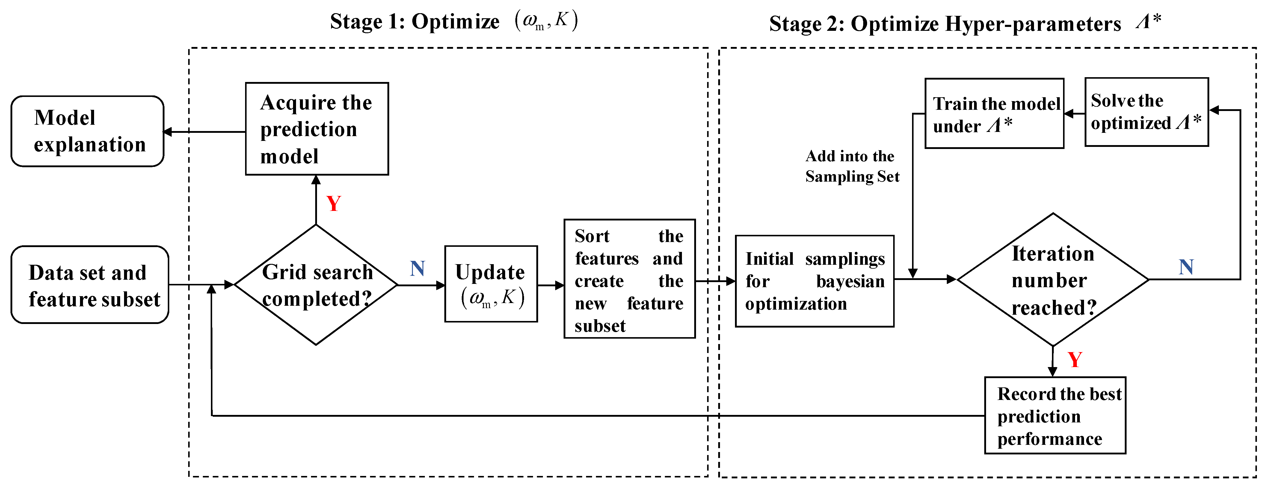
4.1. Model Training and Two-Stage Optimization

The neural network model is utilized as the prediction model, and the accuracy of the model prediction is assessed using the root mean square error on the validation set. The expression is as follows:

$$RMSE=\sqrt{{\displaystyle \frac{1}{N}}{{\displaystyle \sum _{i=1}^N\left(\frac{y_{pred}-y_{true}}{y_{true}}\right)}}^2}$$

(18)

where N is the number of samples in the validation set, y_pred is the predicted value, and y_true is the groundtruth value.

Similar to the aforementioned ω_m and K, machine learning models themselves also contain numerous hyperparameters, which have a significant impact on the accuracy of the model, such as the learning rate, number of hidden layers, number of neurons, and maximum iteration times of neural network models. Hyperparameter optimization is an important means of improving the prediction ability of the model; therefore, the Bayesian optimization method based on tree Parzen estimation is adopted to tune these parameters [28].

It is worth noting that the fusion weighting coefficient ω_m and the feature subset length K are also hyperparameters that need to be optimized; however, they belong to the feature selection stage and have a greater impact on data mining than the hyperparameters of the machine learning model. Therefore, this paper proposes a two-stage optimization method.

In the first step, for any ω_m = ω and K = k, the Bayesian optimization method mentioned above is used to optimize the prediction model hyperparameters until the preset number of iterations P is reached, as shown in Equation (19).

$${\mathcal{l}}_P\left(\omega ,k\right)=\underset{\Lambda }{\min }RMS{E}_{\omega ,k}\left(\Lambda \right)$$

(19)

where RMSE_ω,k represents the root mean square error of the model with fusion weighting coefficient ω_m and feature subset length K.

In the second step, grid search is performed on ω_m and K, continuously changing the fusion weighting coefficient and feature subset length at a specific resolution to minimize ${\mathcal{l}}_P\left(\omega ,k\right)$. After solving the optimal values of ω_min and k_min, the corresponding feature subset is determined, and the optimal model will be utilized as the prediction model. The flowchart of the two-stage optimization process is shown in Figure 4. In this paper, P is set to 200.

$${\omega }_{\min },k_{\min }=\arg \min {\mathcal{l}}_P\left(\omega ,k\right)$$

(20)

4.2. Model Explanation

Due to the nature of machine learning models, prediction models are essentially black box models. In order to enhance the post hoc explainability, model explanation methods are carried out based on SHAP analysis partial dependence plots. Among them, partial dependence plots can be used to explore the rules of the target variable y as any feature x changes. This method estimates the expectation of the prediction value by the Monte Carlo method and evaluates the marginal effect of any single feature on the prediction value. The expression is as follows:

$$f\left(x_i\right)={\displaystyle \frac{1}{N}}{\displaystyle \sum _{k=1}^{N}v\left(x_i,{\mathit{x}}_{~i,k}\right)}$$

(21)

where f represents the impact of a single feature on the prediction value, v represents the prediction model, x_i represents the feature to be analyzed, while x_~i,k represents the collection of features excluding x_i in the k-th sample.

The SHAP method [29,30] is based on the Shapley value, which analyzes the contribution of each feature to the model’s prediction results. The Shapley value calculates the feature contribution by averaging the prediction differences when considering all feature combinations with and without the i-th feature. The expression for the Shapley value is shown in the following equation:

$$\mathrm{\Phi }\left(v\right)={\displaystyle \sum _{S\subseteq X\backslash \left\{x_i\right\}}\frac{1}{C\left(\left|X\right|-1,\left|S\right|\right)}}\left[v\left(S\cup \left\{x_i\right\}\right)-v\left(S\right)\right]$$

(22)

where C (*,*) represents the combination function, and v(S) represents the prediction value of the feature subset S under a certain input. However, directly calculating the Shapley value of a machine learning model poses many difficulties. The biggest problem is that the machine learning model is unable to predict feature subsets. For example, after training a machine learning model y = F(X), it cannot be directly used to predict y′ = F(X\{x_i}). This also makes it impossible to calculate Equation (22). If a machine-learning model is trained for all feature subsets of X, it will require training 2^|X| times, which is unacceptable. To solve this problem, the SHAP method introduces the Local Interpretable Model-agnostic Explanation (LIME) method, which constructs a multivariate linear surrogate model near the given input parameters and proposes a “simplified input” x_i′ that can represent whether feature x_i is removed from the feature set, achieving the prediction of any feature subset of a black box model. The expression of the surrogate model is shown in Equation (23).

$$f\left(X\right)=g\left(X^{\prime }\right)={\varphi }_0+{\displaystyle \sum _1^{\left|X^{\prime }\right|}{\varphi }_i{x}_i^{\prime }}$$

(23)

In the equation, X′ represents the “simplified input” of the original feature set X. When the feature subset to be predicted contains x_i, x_i′ = 1; otherwise, x_i′ = 0. Furthermore, the mapping function h_X(X′) = X is defined to represent the mapping relationship from X′ to X. The expression of ${\varphi }_i$ in Equation (23) is as follows:

$${\varphi }_i={\displaystyle \sum _{Z^{\prime }\subseteq X\prime }\frac{\left|Z^{\prime }\right|!\left(\left|X^{\prime }\right|-\left|Z^{\prime }\right|-1\right)!}{\left|X^{\prime }\right|!}}\left[f\left(h\left(Z^{\prime }\right)\right)-f\left(h\left(Z^{\prime }\backslash z_i^{\prime }\right)\right)\right]$$

(24)

where Z′ is a subset of X′. To address the problem of machine learning methods unable to predict feature subsets, assuming that the features are independent of each other, the predicted values can be estimated as follows:

$$f\left(h\left(Z^{\prime }\right)\right)\approx f\left[h\left({\mathit{Z}}_s^{\prime }\right),E\left(Z^{\prime }\backslash {\mathit{Z}}_s^{\prime }\right)\right]$$

(25)

where Z_s′ represents the set of non-zero elements in Z′. Under the assumption of feature independence, the expected value of the prediction for the set of zero elements (representing the unselected feature set) $E\left(Z^{\prime }\backslash {Z^{\prime }}_s\right)$ can be estimated through sampling. When interpreting the model, the SHAP values for all features are first calculated for each sample, and the influence of each feature on the prediction value when it changes around the mean is observed, that is, ${\varphi }_i$. Finally, take the average of the SHAP values of all samples on every feature to obtain the corresponding feature contribution under different inputs, as shown in Equation (26).

$$\overline{{\varphi }_i}={\displaystyle \frac{1}{N_s}}{\displaystyle \sum _{i=1}^{N_s}\left|{\varphi }_{i,k}{x}_i^{\prime }\right|}$$

(26)

5. Case Studies and Discussion

5.1. Validation of the Feature Selection Method Using Synthetic Data

The hybrid feature selection method is the core of this work. Due to the complexity of the engine product and limited testing accuracy, it is important to verify the performance and applicability of the hybrid feature selection method under different simulation deviations, cognitive biases, and data noise combinations, especially considering that the knowledge-based metric is usually subjective. This paper uses a synthetic data set generated by a high-fidelity simulation model with known important features. A simulation model of a rocket engine pressurization system is selected as the data set generator, as shown in Figure 5a. The system has a main route and a sub-route for pressurization. The main route is always open during flight, while the sub-route uses Bang-Bang control to regulate the tank pressure. A typical pressurization process is shown in Figure 5b. Due to the use of a Bang-Bang controller to regulate the pressure inside the tank, the solenoid valve will repeatedly open or close, causing the sealing surface to constantly collide and the leakage rate to gradually increase. Therefore, based on the synthesized data, we selected the expected leakage rate of the solenoid valve as the observed parameter of the synthesized data set and 18 product parameters as the manufacturing parameters. We used reliable engineering experience and the proposed hybrid feature selection method with different types of noise to rank the 18 features. The difference between the feature rankings obtained by the feature selection method and the known important feature rankings is calculated as the evaluation metric to analyze the applicability of the hybrid feature selection method under noise.

The high-fidelity mathematical model for the pressurization system is shown in Equations (27)–(30):

$$C_{\mathrm{v}}{m}_{\mathrm{u}}{\displaystyle \frac{\mathrm{d}{T}_{\mathrm{u}}}{\mathrm{d}t}}={\displaystyle \sum _{i=1}^N{C}_{\mathrm{p}}{T}_{\mathrm{i}}\frac{\mathrm{d}{m}_i}{\mathrm{d}t}-}{C}_{\mathrm{v}}{T}_{\mathrm{u}}{\displaystyle \frac{\mathrm{d}{m}_{\mathrm{u}}}{\mathrm{d}t}}-p_{\mathrm{u}}{\displaystyle \frac{\mathrm{d}{V}_{\mathrm{u}}}{\mathrm{d}t}}-{\displaystyle \sum _{k=1}^N{Q}_k}$$

(27)

$$p_{\mathrm{u}}{V}_{\mathrm{u}}=Z·m_{\mathrm{u}}R{T}_{\mathrm{u}}$$

(28)

$${\displaystyle \frac{\mathrm{d}{m}_{\mathrm{ev}}}{\mathrm{d}t}}={\displaystyle \frac{V_{\mathrm{u}}}{R_{\mathrm{v}}{T}_{\mathrm{u}}}}{\displaystyle \frac{\partial (P_{\mathrm{vg}}-P_{\mathrm{vc}})}{\partial t}}$$

(29)

$$Q=AT+Bu$$

(30)

where p_u, V_u, T_u, and m_u are the pressure, volume, temperature, and mass of ullage in the gas chamber (such as gas bottle or tank); m_i and T_i represent the mass and temperature of the inflowing gas; C_p and C_v are the specific heat capacities of the pressurization gas at constant pressure and constant volume, respectively; Q_k is the heat transfer term; m_ev represents the mass of the propellant evaporated/condensed; R_v is the gas constant of the propellant vapor; P_vg and P_vc represent the saturated vapor pressure and current partial pressure of the propellant vapor, respectively; Q represents heat exchange power matrix; T is the vector composed of the temperature of all components; u is the temperature of the external heat source or cold source; and A and B are matrices representing the heat transfer paths.

In engineering practice, the sealing reliability of valves and actuators is mainly evaluated by the Weibull distribution, which means that every time the valve is opened or closed, the failure rate of leakage will increase. Therefore, the following equation is used to estimate the expected leakage rate.

$$q_{\mathrm{leak},\exp }=k_{\mathrm{leak}}·n_{\mathrm{toggle}}$$

(31)

where q_leak,exp is the expected leaking mass flow rate of the solenoid valve, k_leak represents the coefficient indicating the reliability of the valve sealing, and n_toggle is the number of times the valve opens or closes.

Specifically, the validation of the hybrid feature selection method is carried out in the following steps:

(1)

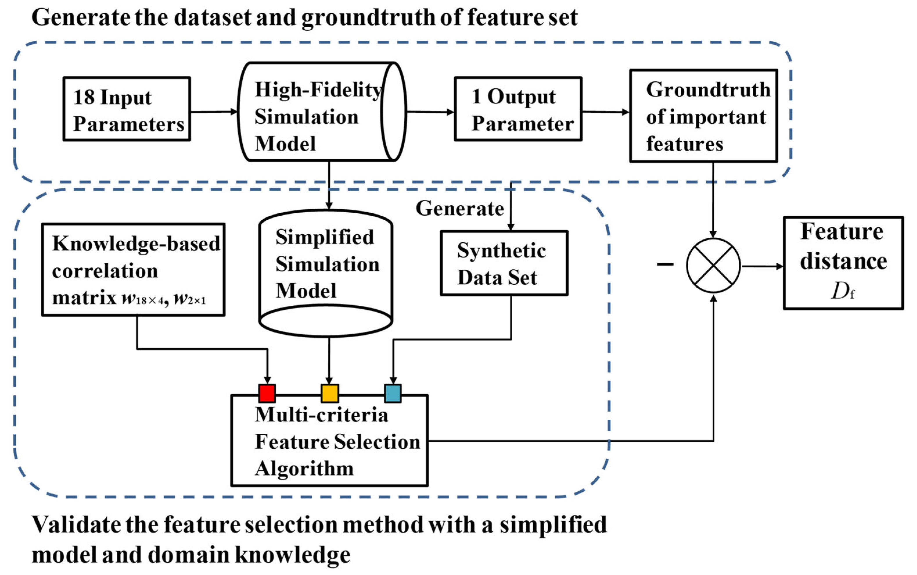
Determine the input parameters (serve as manufacturing process parameters) and output (serve as observed parameters), build the simulation model, and select the prior key features: select 18 parameters as input and the expected leaky rate of the solenoid valve as output. Establish a high-fidelity simulation model of the pressurization system, calculate the time of valve actions, and eventually obtain the expected leaky rate of the solenoid valve. Then select n key features based on reliable engineering experience.

(2)

Generate the data set: determine the fluctuation range of input parameters, use hypercube sampling to form the sampling matrix, and input the simulation model to obtain the training set.

(3)

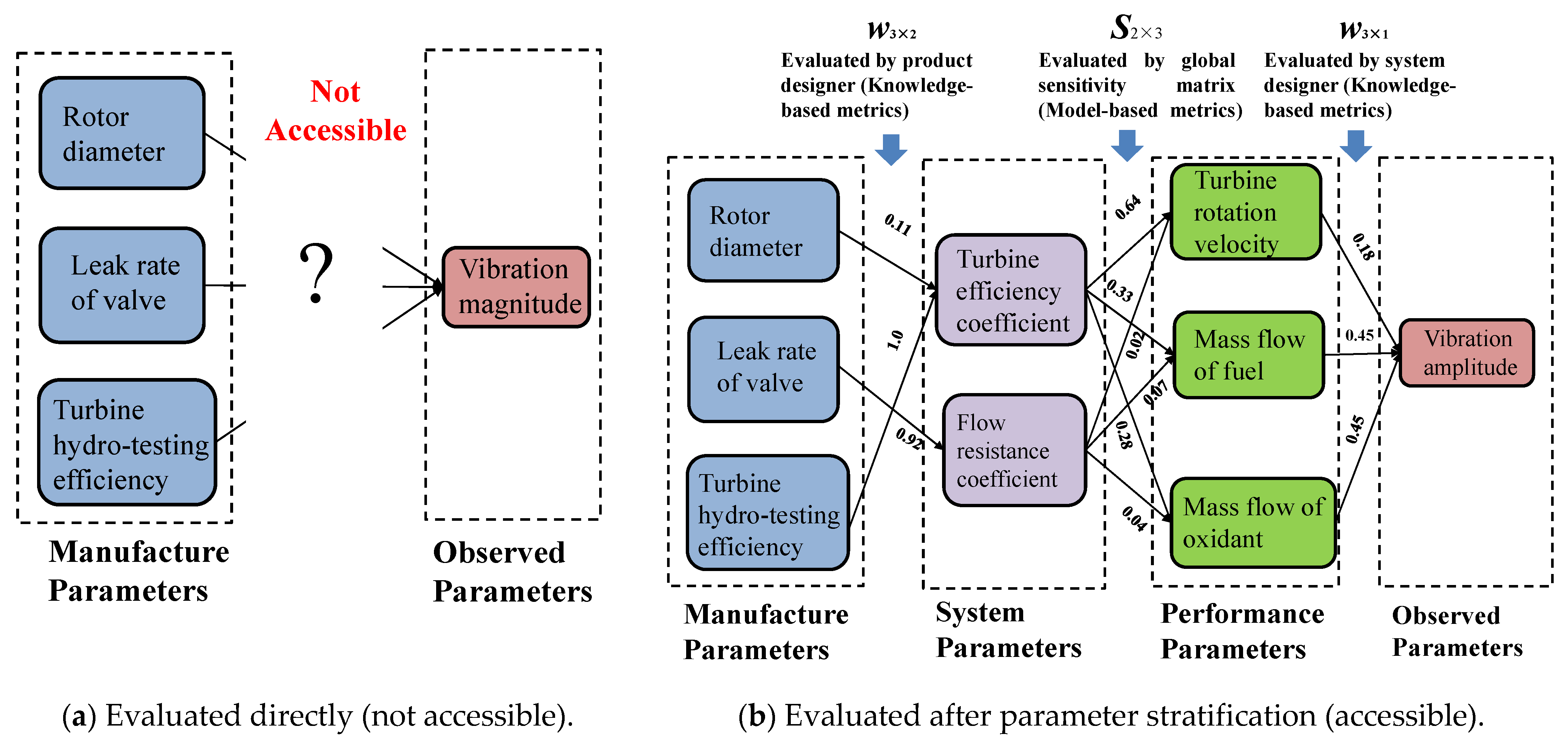
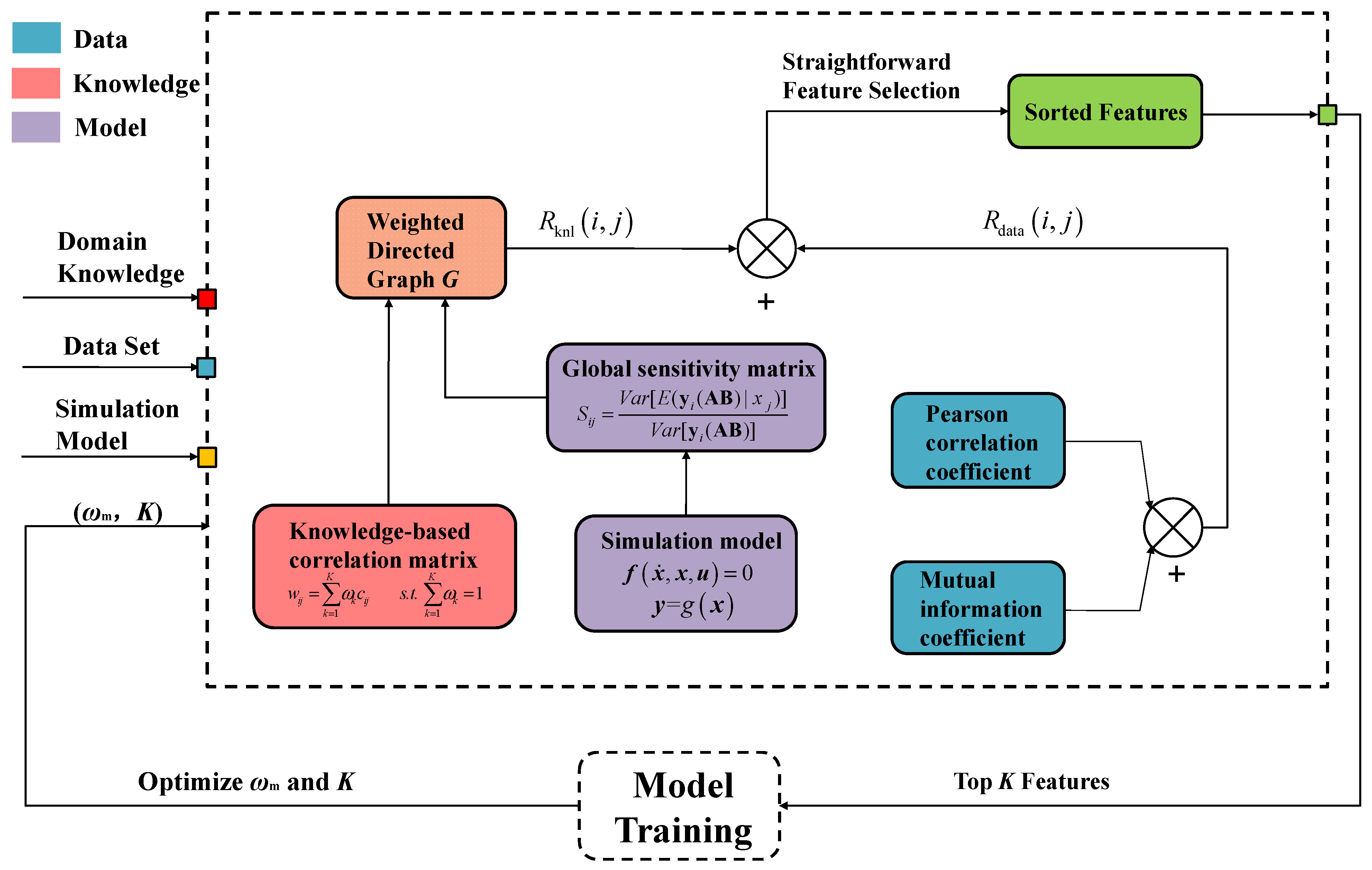
Build the simplified simulation model and three types of correlation matrices: assuming that the high-fidelity simulation model is unknown, construct a simplified simulation model that does not contain all input and output parameters. The simplified model in this paper is shown in Equations (32)–(34).

$${\left({\displaystyle \frac{\mathrm{d}P}{\mathrm{dt}}}\right)}_{\mathrm{up}}={\displaystyle \frac{R_{\mathrm{g}}T}{V}}{\displaystyle \sum \dot{m}}-{\displaystyle \frac{m{R}_{\mathrm{g}}T}{V^2}}{\displaystyle \frac{\mathrm{d}V}{\mathrm{d}t}}+{\displaystyle \frac{m{R}_{\mathrm{g}}}{V}}{\displaystyle \frac{\mathrm{d}T}{\mathrm{d}t}}$$

(32)

$${\left({\displaystyle \frac{\mathrm{d}P}{\mathrm{dt}}}\right)}_{\mathrm{dn}}=-{\displaystyle \frac{m{R}_{\mathrm{g}}T}{V^2}}{\displaystyle \frac{\mathrm{d}V}{\mathrm{d}t}}+{\displaystyle \frac{m{R}_{\mathrm{g}}}{V}}{\displaystyle \frac{\mathrm{d}T}{\mathrm{d}t}}$$

(33)

$$t_{\mathrm{R}}=\Delta P_{\mathrm{ctr}}/{\left({\displaystyle \frac{\mathrm{d}P}{\mathrm{dt}}}\right)}_{\mathrm{up}}+\Delta P_{\mathrm{ctr}}/{\left({\displaystyle \frac{\mathrm{d}P}{\mathrm{dt}}}\right)}_{\mathrm{dn}}$$

(34)

where t_r represents the average time for the first opening and closing cycle of the electric valve, and P_ctr represents the pressure control bandwidth. The input of the simplified model is considered as system parameters, and the output is considered as performance parameters. The input parameters and output parameters of the high-fidelity model in step (1) are considered manufacturing process parameters and observed parameters, respectively. Evaluate the correlation between 18 high-fidelity model input parameters and the simplified model input parameters and the correlation between the simplified model output and the solenoid valve life using current engineering experience. Calculate the correlation between the simplified model input and output parameters using model-based global sensitivity analysis, and finally form three types of correlation matrices.

(4)

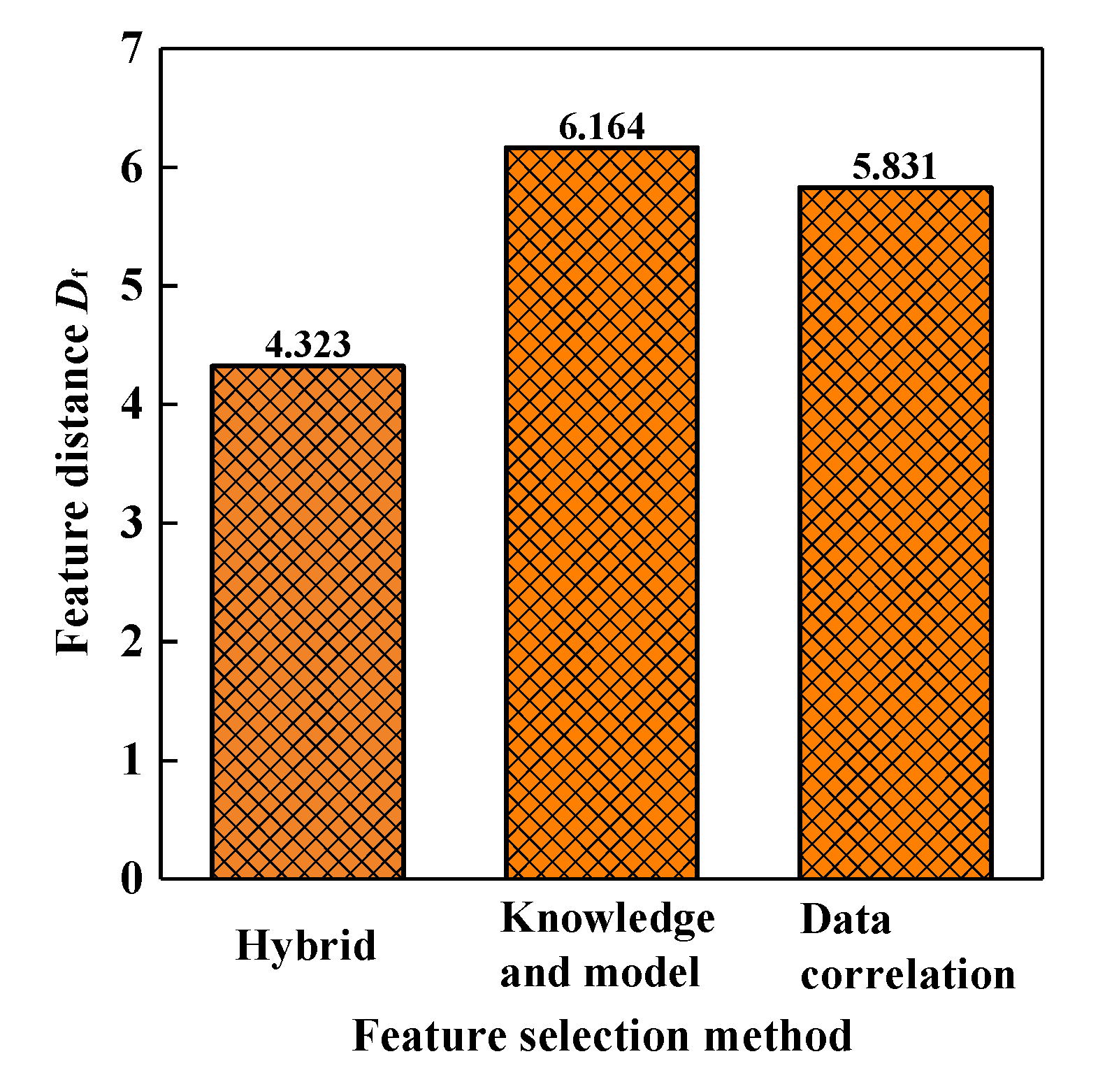
Perform feature sorting and calculate feature selection performance evaluation metrics. Based on the sensitivity matrix and the knowledge-based correlation matrix obtained in the previous step, use different feature selection methods to rank the features (which are the 18 input parameters). Let f_sort be a set composed of the serial numbers of the top n important features after sorting, and calculate the Euclidean distance between f_sort and the groundtruth feature set f_true as the feature sorting performance evaluation metric D_f, as shown in Equation (35). The smaller the feature distance D_f, the closer the feature sorting obtained by the feature selection method is to the groundtruth feature sorting, the better the method performs, and vice versa.

$$D_{\mathrm{f}}={‖f_{\mathrm{sort}}-f_{\mathrm{true}}‖}_2$$

(35)

where f_true = [1, 2, …, n], n is the number of key features. The validation process for feature selection methods is shown in Figure 6.

The configuration of each module in the figure is shown in

Table 2. Configuration of the modules.

Module Name	Module Function	Module Configuration
High-fidelity simulation model consisting of Equations (27)–(30)	Generate synthetic data set and groundtruth feature ranking	18 input parameters and 1 output parameter
Knowledge-based correlation matrix I	Validate the hybrid feature selection method	Size 18 × 4
Simplified simulation model consisting of Equations (32)–(34)		4 input parameters and 2 output parameters, forming the model-based correlation matrix with the size of 4 × 2
Knowledge-based correlation matrix II		Size 2 × 1

.

Following the above steps, first, perform Latin hypercube sampling on the high-fidelity simulation model within the specified range to obtain 3000 sampling points as the data set. Based on the engineering experience of pressurization system design, the diameter of the fuel tank pressurization orifice, the flow resistance constant of the thrust regulator valve, the initial temperature of the gas bottle, and the initial volume of the fuel tank ullage are determined as key features, and their impact on the valve opening time interval decreases in order. The four types of parameters in the data set are shown in Appendix B. Next, assuming that the mathematical model and key features of the system are unknown, a simplified model is built to represent the “simulation model currently recognized” to simulate the data mining process, shown in Equations (32)–(34).

Next, build the knowledge-based correlation matrix (size of 18 × 4, 2 × 1) and model-based sensitivity matrix (size of 4 × 2). Calculate the corresponding feature distances D_f using data-based, knowledge and model-based, and hybrid feature selection methods, as shown in

Table 3. Feature rankings (top 4) obtained by different feature selection methods.

Feature Selection Method	Sorting of the Top 4 Features
Groundtruth ranking	[1, 2, 3, 4]
Knowledge and model-based method	[1, 8, 2, 3]
Data-based method	[1, 5, 3, 9]
Hybrid method	[1, 6, 3, 5]

. It can be seen from Figure 7 that, under ideal conditions (i.e., no noise in the data, no significant errors in domain knowledge, and accurate simulation models), the feature distance of the hybrid feature selection method is slightly smaller than that of the single standard feature selection method. This is because the knowledge-based method underestimated the importance of “the flow resistance constant of the thrust regulator valve”, while the data-based method failed to identify the important feature “initial volume of fuel tank ullage”. After weighting the two metrics, the feature scoring errors of the two methods were complementary, thus improving the feature selection results.

However, in practical engineering, there is a large amount of noise and deviation in knowledge, simulation models, and measurement data. The fusion result cannot be as ideal as above, and it cannot be guaranteed that the bias of the two feature selection methods can offset each other under all data mining tasks. In fact, in many cases, the evaluation errors of the two methods on the same feature may be superimposed, causing the feature selection results to deteriorate. Therefore, it is necessary to evaluate the performance of feature selection methods under noise conditions.

For domain knowledge, the main source of error is cognitive error; that is, engineering experience does not recognize the correlation between a production parameter and a system parameter, or mistakenly believes that there is a correlation between them; for the data side, the error mainly comes from correlation evaluation methods and data errors; that is, the correlation metrics cannot well represent the correlation, or the quality of the data itself is poor; for the simulation model side, the error comes from the bias between the model and the measured data. According to current experience, cognitive bias is the largest, data noise is the second, and model error is the smallest. This is because, for knowledge evaluation, most parameters do not have a suitable evaluation standard for the impact on system parameters, and the correlation is prone to large errors; for simulation models, due to the model calibration methods, the errors can be controlled within a small range. Our previous work [31] showed the effect of model calibration of the propulsion system.

Considering the complex impact of noise on feature distance, the Monte Carlo method is utilized to evaluate the performance and robustness of different feature selection methods under different cognitive, model, and data biases. Based on the above discussion, the noise conditions are defined as follows: model bias is fixed at 0.03, cognitive bias and data noise follow normal distributions with mean values μ_cog ∈ [0, 0.3] and μ_dat ∈ [0, 0.2], respectively. Within the noise space of μ_cog ∈ [0, 0.3] and μ_dat ∈ [0, 0.2], 1000 sets of samples are obtained using uniform sampling, where each sample represents a specific intensity of noise. A total of 1000 random experiments are conducted at each point, and the mean feature distance D_f is calculated. Let ${\overline{D}}_{\mathrm{mix}}$, ${\overline{D}}_{\mathrm{ps}}$, and ${\overline{D}}_{\mathrm{kn}}$ represent the mean D_f values for the hybrid method, data-based method, and knowledge and model-based method, respectively. Contours for ${\overline{D}}_{\mathrm{mix}}-{\overline{D}}_{\mathrm{ps}}$, ${\overline{D}}_{\mathrm{mix}}-{\overline{D}}_{\mathrm{kn}}$, ${\overline{D}}_{\mathrm{mix}}-\min \left({\overline{D}}_{\mathrm{ps}},{\overline{D}}_{\mathrm{kn}}\right)$, and ${\overline{D}}_{\mathrm{mix}}-\max \left({\overline{D}}_{\mathrm{ps}},{\overline{D}}_{\mathrm{kn}}\right)$ are plotted as shown in Figure 8, where the red dashed line represents the contour line with a value of 0. From Figure 8a,b, it can be seen that the hybrid method is superior to the single method in most areas. Compared with the data-based feature selection method, the hybrid method performs better in feature selection performance in areas other than high cognitive bias and low data noise; compared with the knowledge and model-based feature selection method, the hybrid method performs better in areas other than low cognitive bias and high noise error. Figure 8c shows that the hybrid method is not a simple compromise between the two methods. Compared with the best performance of the two single methods, the hybrid method still achieves better feature selection performance in more than one-third of the noise space, especially in the area of low cognitive noise and low data noise. In addition, in areas of low cognitive noise and low data noise, ${\overline{D}}_{\mathrm{mix}}-\min \left({\overline{D}}_{\mathrm{ps}},{\overline{D}}_{\mathrm{kn}}\right)$ is even lower than the case without noise (as shown in Table 3). This indicates that the hybrid method is far less sensitive to noise with lower intensity compared to single methods; Figure 8d shows that the hybrid method has a higher performance lower bound. The performance of the hybrid method in the noise space is always higher than the worst of the two single feature selection methods, which is of great significance in tasks that lack data noise and cognitive bias prior information.

To further explore the applicability of hybrid feature selection methods, the noise space is divided into four parts according to the relationship between cognitive error and data noise. These parts are Ω₁ (low cognitive bias, low data noise), Ω₂ (high cognitive bias, high data noise), Ω₃ (low cognitive bias, high data noise), and Ω₄ (high cognitive bias, low data noise). In practical engineering, Ω₁ to Ω₄ represent different types of products. For example, Ω₁ generally covers simple products such as mechanical valves. These products have less data, complete testing processes, high data quality, and relatively clear mechanisms. Ω₂ and Ω₄ include complex power products led by liquid rocket engines. The production test parameters of such products have a large gap with the product performance level, and the domain knowledge is lacking. The measurement of the data is difficult, and the data resolution and accuracy might be limited. Studying the feature selection performance under different noise intensity constraints is of great significance for guiding data mining work for specific products. First, take a feature point in each of the four regions, where P1 (0.02, 0.02), P2 (0.33, 0.16), P3 (0.03, 0.18), and P4 (0.32, 0.03). The distribution of feature distance D_f at the four feature points was calculated using kernel density estimation.

Figure 9b–e show the fitting results of the feature distance distribution. It can be seen that the hybrid method has the smallest mean at P1 and the largest difference in feature distance distribution among the three methods. At P2, the feature distances of the three methods tend to be consistent and close to a normal distribution, which is due to the high noise level that partially masks the true feature distance distribution. Even so, the performance of the fusion method is slightly better than that of the two single methods. At P2 and P3, the performance of the hybrid method is between that of the two single methods. Mature aerospace products generally do not fall into P3, because, once a feature is identified as a key parameter, the designers will strengthen the testing process for that parameter to meet the testing coverage requirements. As for P4, Equation (17) stipulates that, when the data-based correlation is higher than a certain threshold, the data correlation will be used directly instead of the fusion correlation as the feature evaluation index, avoiding significant performance degradation of the fusion method at P4. The above results verify the applicability of the fusion method in different types of aerospace products.

Further investigation was conducted on the impact of fusion weighting coefficient ω_m on the hybrid feature selection method. The improvement coefficients r_i,min and r_i,max is defined as the ratio of the area in the noise space Ω_i where the feature distance for the hybrid method is smaller than the minimum/maximum feature distance for the two single methods, to the total area of the noise space Ω_i, as shown in (36)~(39). A larger r_i,min value means that, within this noise space, the hybrid method is more likely to obtain feature selection results that are more consistent with the groundtruth feature ranking. Since the performance of the hybrid feature selection method is better than any single feature selection method in the area of ${\mathrm{\Omega }}_i\cap D-D_{\min }<0$, this area is defined as the “high-performance region”.

$$r_{i,\min }={\displaystyle \underset{{\mathrm{\Omega }}_i\cap D-D_{\min }<0}{\iint }\mathrm{d}S}/{\displaystyle \underset{{\mathrm{\Omega }}_i}{\iint }\mathrm{d}S}$$

(36)

$$r_{i,\max }={\displaystyle \underset{{\mathrm{\Omega }}_i\cap D-D_{\max }<0}{\iint }\mathrm{d}S}/{\displaystyle \underset{{\mathrm{\Omega }}_i}{\iint }\mathrm{d}S}$$

(37)

$$D_{\max }=\max \left(D_{\mathrm{kn}},D_{\mathrm{ps}}\right)$$

(38)

$$D_{\min }=\min \left(D_{\mathrm{kn}},D_{\mathrm{ps}}\right)$$

(39)

Figure 10 shows the trends of r_i,min and r_i,max of regions Ω₁ to Ω₄ under different fusion coefficients ω_m. It can be observed from Figure 10a and Figure 11 that, with an increase in ω_m, the high-performance region gradually rotates towards the direction of high data noise, leading to a decrease in the performance in the high cognitive error region but an improvement in performance in the high data noise region. Among the four regions, the effect of ω_m on the feature selection performance is the smallest in the low cognitive noise and low data noise area, maintaining consistently high performance. However, in the regions of extremely high cognitive error and low data noise, as well as extremely high data noise and low cognitive noise (corresponding to P3 and P4 in Figure 9), the performance is consistently poor. From Figure 10b, it can be seen that, when ω_m is between 0 and 1, the performance of the hybrid feature selection method is always better than that of the single feature selection method with poorer performance. This further illustrates that, under the condition of lacking prior information on cognitive bias and data noise, the hybrid method has better robustness.

In summary, the performance of the hybrid feature selection method can be concluded as follows: (1) The hybrid feature selection method is always better than one of the two single methods with poorer performance. Under specific noise conditions, it outperforms any single method, especially in tasks with low cognitive errors and low data noise. The performance of the hybrid feature selection method is between the two single feature selection methods when there is a large difference in cognitive errors and data noise. Moreover, the larger the difference, the less likely the hybrid method is to achieve the best results. As the increase of ω_m, the high-performance region gradually rotates towards the direction of larger data noise. (2) The above conclusion also validates the rationality of the feature subset selection method proposed in Section 3.3. First, the change of ω_m leads to the movement of the high-performance region, so using the wrapper method to determine ω_m can avoid subjective judgment errors and affect the reliability of feature selection. Secondly, as mentioned earlier, the combination of cognitive bias and data noise in rocket engine products generally falls into the Ω₂ and Ω₄ regions. In these regions, the hybrid method’s performance significantly deteriorates in areas with extremely low data noise and high cognitive bias. Therefore, when the data correlation is higher than a certain threshold (usually indicating less data noise or the correlation metric can well describe the relationship between parameters), directly using data correlation as the correlation evaluation metric effectively expands the high-performance region and enhances the applicability in rocket engine products.

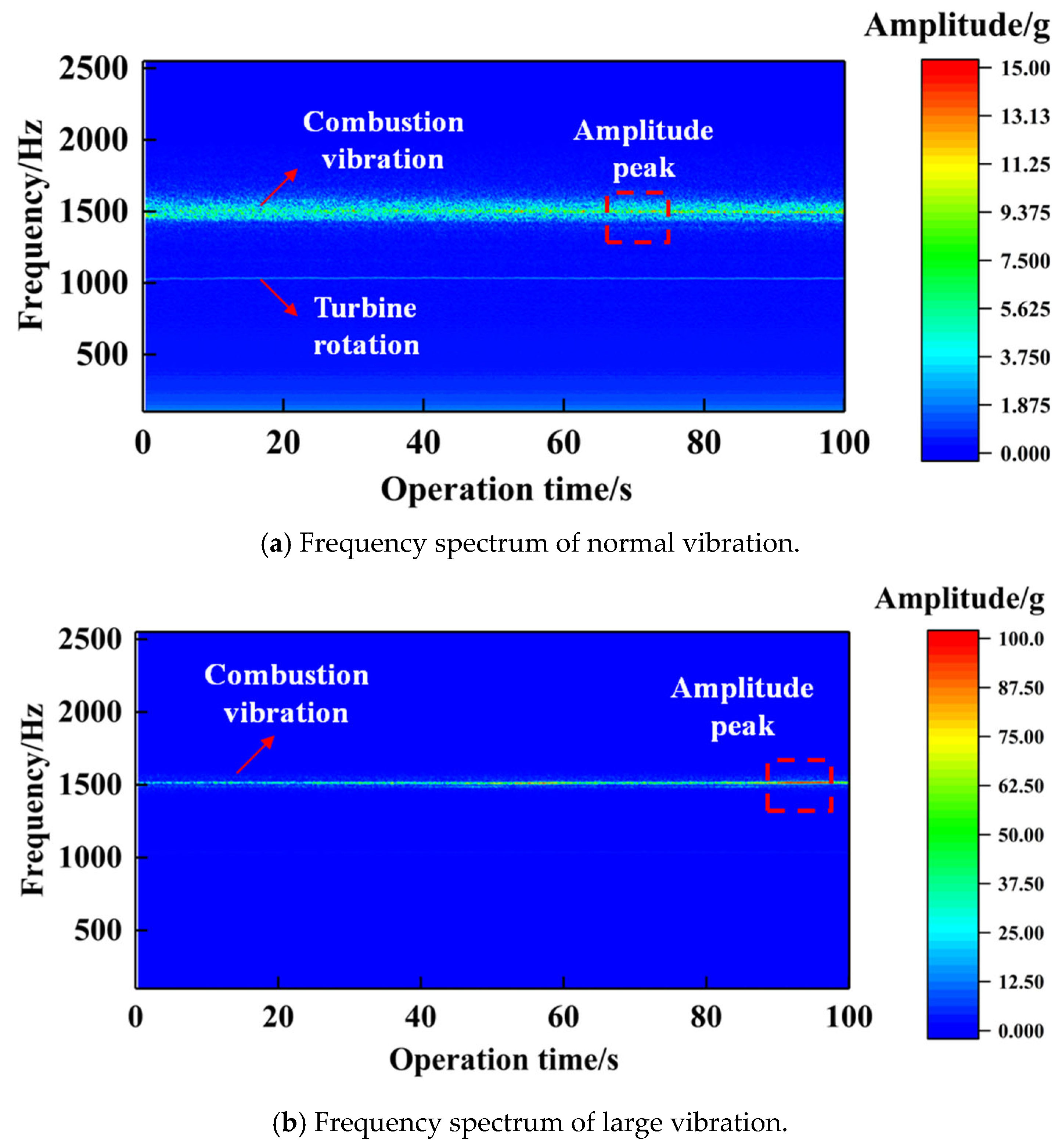
5.2. Data Mining of Large Vibration in an Active Rocket Engine

The system structure of a certain active rocket engine is shown in Figure 12, and the abbreviations of some components are shown in

Table 4. Rocket engine components and their abbreviations.

Component Names	Abbreviations
SFV	Sub-system fuel Venturi tube
MFV	Main system fuel Venturi tube
SOO	Sub-system oxidant orifice
SOV	Sub-system oxidant Venturi tube
MOV	Main system oxidant Venturi tube
CJ	Cooling jacket

. This is an open-cycle engine with room-temperature propellants. Its vibration sensor has a frequency measurement range of 10 Hz~5120 Hz and a maximum acceleration amplitude of 200 g. The vibration sensor is welded to the top of the thrust chamber to measure high-frequency vibration signals in the engine’s axial direction (consistent with the direction of the thrust line). Since the vibration amplitude in this direction is much greater than in the other two directions, it can properly characterize the vibration characteristics of the engine.

Based on past flight data, large vibration sometimes occurs during the engine working process, which is reflected in the large root mean square value at the peak frequency. This paper conducts data mining on this phenomenon.

Figure 13a,b shows the frequency spectrum diagrams of axial acceleration signals at the engine combustion chamber during two flight tests. Figure 13a represents normal vibration amplitude, while Figure 13b represents excessive vibration amplitude. From the spectral analysis result, the large vibration amplitudes are concentrated around 1000 Hz and 1500 Hz, with the maximum acceleration amplitude occurring at 1500 Hz. Additionally, 1000 Hz represents twice the turbo-pump rotational frequency (speed approximately 30,500 rpm), while 1500 Hz is the combustion frequency. Near 1500 Hz in Figure 13b, the maximum acceleration amplitude is approximately 105 g/Hz, with an average amplitude of about 25.5 g/Hz, where the maximum amplitude is about 7 times that of Figure 13a (15.0 g/Hz), and the average amplitude is about 12 times that of Figure 13a (2.1 g/Hz), while there is no significant difference in amplitude at 1000 Hz. From this analysis, it can be concluded that the 1500 Hz excitation, namely, combustion instability, is the main cause of excessive engine vibration. The knowledge graph in this case study is constructed based on vibration caused by combustion instability, and the maximum root mean square value of acceleration amplitude (maximum RMS) is selected as the parameter characterizing engine vibration.

Telemetry data from 124 engines launched or tested in recent years were selected, with 102 used as the training set and 22 used as the validation set. Based on manufacturing, testing, flight telemetry data and rocket design knowledge, 88 parameters were selected, including 47 manufacturing process parameters, 28 system parameters, 16 performance parameters, and 1 observed parameter (see Appendix A); correlation matrices based on expert knowledge (47 × 28, 16 × 1) and simulation model sensitivity (28 × 16) were formed. Among them, the feature numbers of production process parameters are F0 to F46, where F0 to F15 and F46 are hydraulic testing data, and the others are dimension chain data, leak detection data, etc. It is worth noting that, for knowledge metrics between the performance parameters to the observed parameter, due to the lack of prior knowledge and the fact that vibration sensors are installed at the thrust chamber head, all parameters related to thrust chamber combustion (thrust chamber flow rate, thrust chamber mixture ratio, injection pressure, injection pressure drop, etc.) were set to have a correlation of 0.8 with the observed parameter (maximum RMS), while parameters related to the gas generator combustion (sub-system mixture ratio, sub-system flow rate, etc.) were set to have a correlation of 0.7 with the observed parameter(maximum RMS). In terms of software, a data pre-processing module, feature selection module, Bayesian optimization module, and model explanation module were developed based on Python 3.8. A parameterized neural network training module was built based on the deep learning framework Pytorch 1.6. A high-fidelity rocket engine simulation model and a pressurization system simulation model were developed using the MWorks 2024 multidisciplinary simulation platform and coupled with Python through FMU.

Firstly, feature selection is performed. Figure 14a–d show the top 15 features obtained by the straightforward feature selection algorithm with fusion weighting coefficients ω_m of 0, 0.4, 0.7, and 1.0. It can be observed that, as ω_m increases, the score of hydraulic testing parameters (F0~F15 and F46) significantly increases. This is because hydraulic testing parameters have an explicit impact on system parameters, and their knowledge-based scores are higher compared to dimensional chain data and leak detection data. Feature F0 (hydraulic testing pressure drop of thrust chamber oxidant injector) and F1 (hydraulic testing pressure drop of thrust chamber fuel injector) rank in the top 2 for all four ω_m, while features F2, F4, F7, F11, and F15 rank in the top 15 for all four ω_m. These parameters can be preliminarily considered as important features that determine engine vibration amplitude.

Figure 15 shows the Spearman correlation coefficients between the ranking for 46 features at ω_m = 0~0.8 and ω_m = 1. A higher correlation coefficient indicates a closer similarity in feature ranking. It can be seen that, at ω_m = 1 and ω_m = 0, the correlation coefficient is only 0.28, indicating a certain difference between the data-based correlation and the knowledge and model-based correlation. Furthermore, to study the difference between the data-based correlation and the knowledge and model-based correlation for different features and target values, the difference in the ranking number of each feature under the conditions of ω_m = 1 and ω_m =0 is calculated. The larger the absolute value of the difference, the greater the contradiction between the data-based correlation and the knowledge and model-based correlation. The 10 features with the most significant differences are shown in Figure 16. It can be seen that, except for F3 (diameter of the thrust chamber throat), the knowledge and model-based correlation of other hydraulic testing parameters is generally higher than the data-based correlation. Although throat diameter is a hydraulic testing parameter, the purpose of the test is to measure dimensions more accurately rather than obtain flow resistance characteristics.

Next, the two-stage optimization method proposed in this paper is adopted to determine ω_m and the feature length K. Let ω_m be 0, 0.1, 0.2, …, 1, with a total of 11 values. Under each value, take the top 2–15 features as the input for training the prediction model, resulting in 11 × 14 = 154 training cases. Each training case uses Bayesian optimization to tune the hyperparameters with 200 iterations and records the lowest root mean square error value. The calculation results are shown in Figure 17a. In the heatmap, the value in the ith row and jth column represents the root mean square value of the optimized prediction model when ω_m = (i − 1)/10 and the K = j + 1.

To observe the distribution of prediction performance under different values of ω_m and number of features, box plots were drawn for each row and column of data in the heatmap, as shown in Figure 17b,c. It can be seen that, when ω_m = 0.2, the overall prediction accuracy is significantly better than other values, and the best prediction accuracy for ω_m = 0.1, 0.2, 0.3, 0.5 and 0.7 are all higher than the cases of ω_m = 0 and ω_m = 1, demonstrating the superiority of the knowledge data fusion feature selection method. On the other hand, as the number of features increases, the overall trend of prediction performance shows an initial improvement followed by a decline.

Based on the above, the model with the highest prediction accuracy is selected as the final prediction model. At this time, ω_m = 0.2, with six features including the hydraulic testing pressure drop of thrust chamber oxidant injector (F0), hydraulic testing pressure drop of thrust chamber fuel injector (F1), hydraulic testing pressure drop of gas generator oxidant injector (F4), oxidant pump hydraulic testing lift (F11), hydraulic testing pressure drop of thrust chamber body (F2), and rotor imbalance torque (F15). Figure 18 compares the predicted values with the measured values, which align well with the line y = x with a root mean square error of 0.168, indicating no significant overfitting.

Figure 19 shows the maximum weighted path of the selected six features in the weighted directed graph, reflecting the inference process of the selected features to the observed parameter. From the R_knl ranking on the left side of the parameters, the knowledge and model correlations of the six selected features are all within the top 11, among which features ranked 1st (F0, F1), and 3rd (F4) were all selected. This result quantitatively demonstrates that the selected features’ compatibility with engineering experience ranks at the forefront among all features. Specifically, features related to flow resistance characteristics (F0, F1, F2, F4) affect the combustion chamber vibration by changing the pressure drop of the propellant through the corresponding components, which in turn affects the pressure balance and changes the pressure drop at the injector. The pressure drop at the generator and thrust chamber is highly correlated with the flow resistance coefficients and has a high knowledge and model-based score. Although the pressure drop in the thrust chamber body can affect the pressure before the injector, the sensitivity of the pressure before the injector to this parameter is low. The rotor parameters (F15, F11) affect the power balance of the pump by changing the rotor efficiency and lift characteristics, which ultimately affect the parameters such as the pressure before the injector. The hydraulic testing lift of the oxidant pump affects the pump efficiency constant and has a certain influence on the flow rate, mixture ratio, and pressure before the injector of fuel and oxidant. A high rotor imbalance may cause radial vibration of the turbine blades or contact with the casing, changing the first-order term of the pump efficiency constant and causing changes in flow rate and pressure at various locations. Although the pressure before the injector is highly sensitive to the pump efficiency constant, the relationship between the pump efficiency and the rotor imbalance is not very clear. Only occasional traces of contact were found during ground hot commissioning, so the knowledge-based score of this feature is not high.

Therefore, the feature selection results conform to the physical mechanism, and the prediction model has both accuracy and explainability. Next, this model will be used for model interpretation.

Figure 20 shows the correlation of the selected features. As can be seen, the average correlation of the six features is 0.118, indicating that the overall correlation between features is relatively low. However, due to the moderate correlation between F0 and F1 (correlation coefficient 0.58), in order to prevent feature correlation from causing fluctuations in SHAP values, 100 sets of inputs were sampled under the training data set distribution, and the mean value of the corresponding SHAP scores was calculated. Figure 21 represents the SHAP analysis results of the prediction model. In Figure 21a, the color variation represents the magnitude of the feature values. The Y-axis represents the ranking of feature importance, with higher values indicating greater importance. The X-axis represents the magnitude of feature SHAP values. If the SHAP value at a certain point is greater than 0, it indicates that the feature contributes positively to the predicted amplitude of the sample point. Conversely, if it is smaller than 0, it contributes negatively. In Figure 21b, the mean values of SHAP scores are shown. From the analysis, it can be observed that, for predicting engine vibration amplitude, the contribution ranking of features is F0 > F4 > F15 > F1 > F2 > F11. Among these, F2, F4, and F15 show a uniform color change, indicating that the impact of these features on the amplitude is approximately monotonic. On the other hand, F0 shows a distinct mixture of red and blue in the non-zero region, implying the presence of significant maximum/minimum points within that range.

Figure 22a–f show the partial dependent plots of the six features’ variation on the vibration amplitude variation in the engine. The solid line represents the mean value, while the dashed line and shadow represent the 95% confidence interval. It can be observed that, as the hydraulic testing pressure drop of the thrust chamber oxidant injector and gas generator injector increases, the predicted max RMS initially declines slightly and then rises significantly. The influence of the hydraulic testing pressure drop of the thrust chamber fuel injector and the hydraulic testing pressure drop of the gas generator oxidant injector on the predicted max RMS is similar, but the impact is lower than that of the oxidant injector. The hydraulic testing pressure drop of the thrust chamber body has a relatively small impact on the predicted value, showing a trend of initially increasing and then slightly decreasing. The predicted max RMS is also relatively insensitive to the oxidant pump hydraulic testing lift and rotor imbalance torque. As these two features increase, the predicted value shows a trend of slowly decreasing and a trend of first decreasing and then slowly increasing, respectively. In terms of the confidence interval, the range for the hydraulic testing pressure drop of the thrust chamber oxidant injector is the narrowest, indicating that it is the dominant factor affecting the predicted value. The confidence interval range for the rotor imbalance torque is the widest, indicating interactions with other features and being more easily influenced by other production process parameters.

According to the above analysis, the following improvement was applied to the engine: during the manufacturing process of oxidant and fuel injectors, an abrasive flow machining process was adopted to control the flatness of the injector disk to less than 0.05 mm and improve the roughness of injection holes; the oxidant injector hole diameter was increased by 0.002 mm. These changes resulted in a slight decrease in fuel/oxidant injector pressure drop (<0.005 MPa), causing changes in features F0 and F1.

Next, the maximum RMS values from flight tests before and after improvements were collected. The sample size after improvements is 40. The statistical results are shown in Figure 23a–c. From histograms 23a,b, it can be seen that there is a notable increase in the proportion of products with maximum RMS values less than 40 g²/Hz; the proportion of products with maximum RMS values greater than 100 g²/Hz slightly decreased, and no products exceeded 120 g²/Hz. From box plot 23c, it can be observed that the engine vibration amplitude shows a clear skewed distribution. Through Mann–Whitney U testing, it was found that there was no significant difference in the median maximum RMS values between engines before and after improvement. However, the mean value was decreased by 3.02 g²/Hz.

The above test results indicate that a slight reduction in oxidant injection flow resistance helps reduce extreme vibration cases, validating the method’s rationality and engineering application prospects and providing a basis for subsequent engine performance optimization. Notably, since the hydro-test pressure drop of the oxidant injector is affected by multiple process and test parameters, such as injection hole roughness and flow velocity, some of these parameters cannot be measured. This suggests that the hydro-test pressure drop of the oxidant injector may serve as an intermediary parameter for these potential factors’ influence on engine vibration. Therefore, future work will be conducted in two parts: 1. Develop high-precision manufacturing parameter measurement (or soft measurement) methods to enrich features of data mining, improve measurement accuracy and resolution, and support the training of more accurate prediction models. 2. Continue to study the manufacturing and process parameters affecting the hydro-test pressure drop of oxidant injectors, analyze these parameters’ mechanistic effects on combustion instability through simulation and testing methods, and improve the knowledge graph.

6. Conclusions

An explainable data mining method for identification of root causes of liquid rocket engine anomalies that integrates data, model, and knowledge is proposed. The results showed that

(1)

Under different combinations of cognitive biases of knowledge and data noise, the hybrid feature selection method is always superior to one of the two single methods with poorer performance and performs better than any single method under specific noise conditions. However, the performance is not good when there is a large difference in magnitude between the two kinds of noise. In addition, as ω_m increases, the high-performance region of the fusion feature selection method gradually moves towards the direction of larger data noise.

(2)

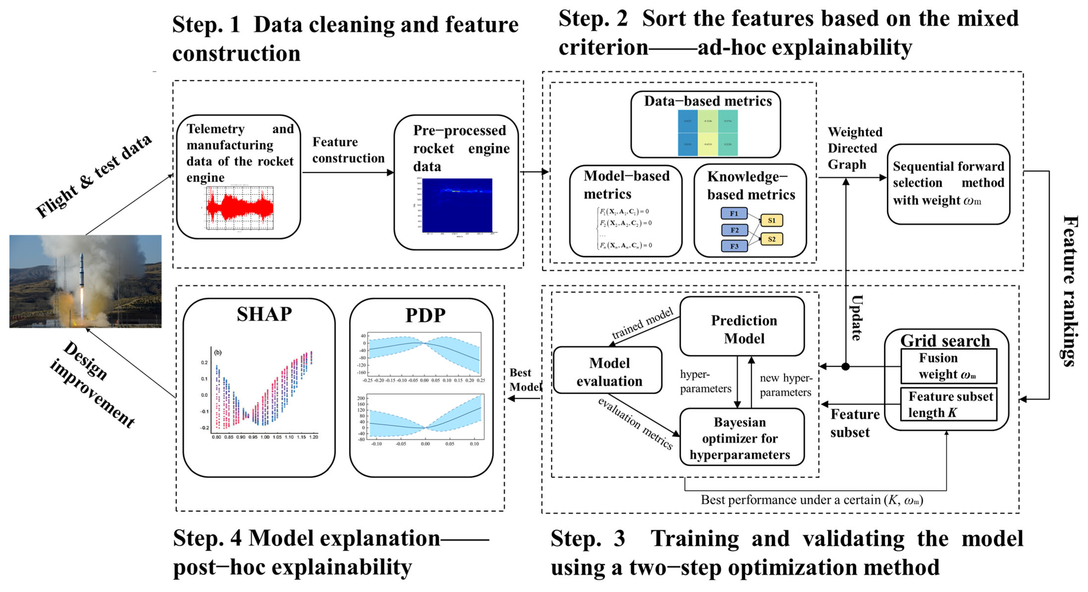
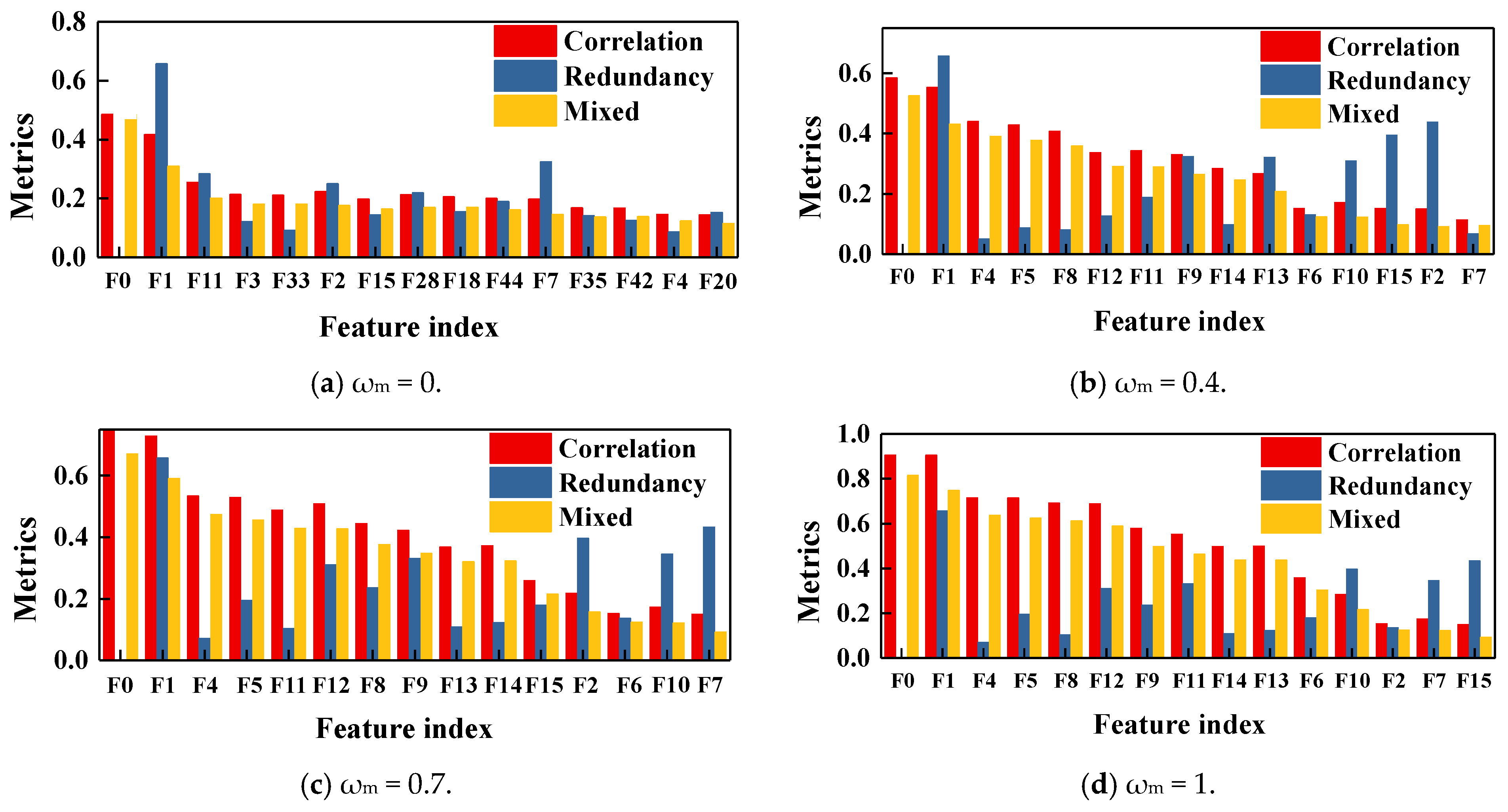
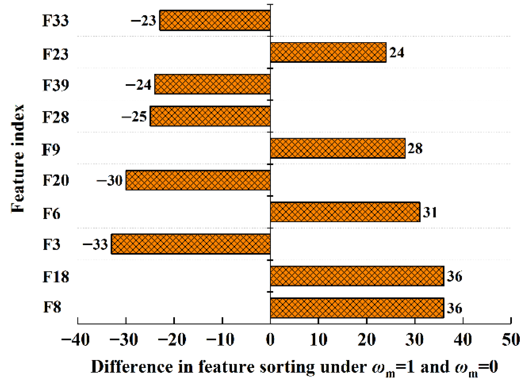
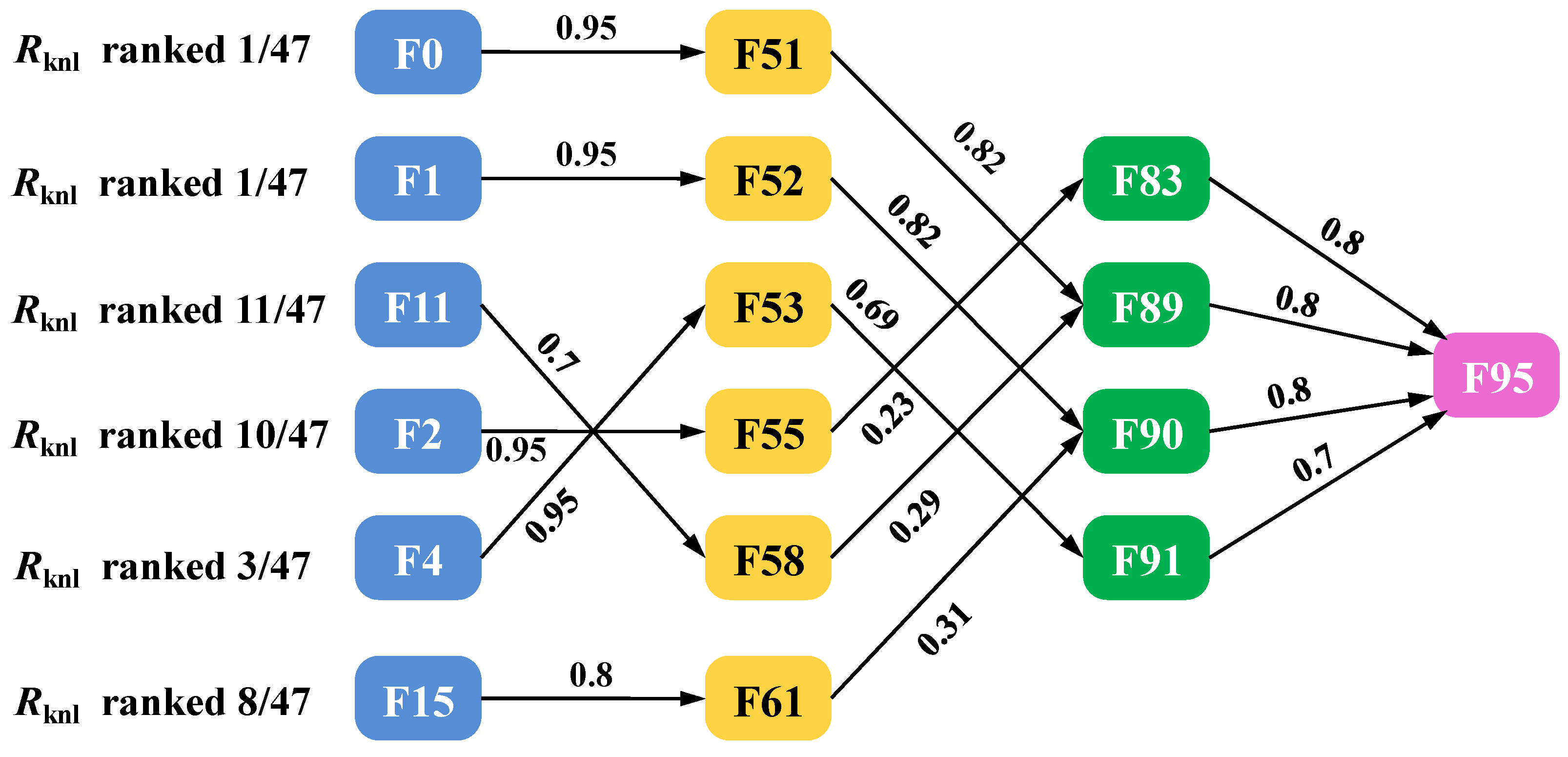
Analysis of the data of a certain active engine shows that there are significant differences between the feature selection result based on existing expert knowledge (ω_m = 0) and the feature selection result based on data correlation (ω_m = 1). As the knowledge and model weight ω_m gradually increase, the ranking of features related to hydraulic testing significantly grows. This indicates that the knowledge and model methods pay less attention to the data, such as dimension chain data and leaking rate data, making it easier to overestimate the importance of hydraulic testing data. By traversing the values of fusion coefficient ω_m and the length of the feature subset K, when ω_m = 0.2 and K = 6, the root mean square error of the prediction model is the lowest (0.168). According to the knowledge and data graph, all of the selected features have a clear mechanism towards the large vibration phenomenon, and model and knowledge-based correlation metrics of these features ranked in the top 25% of all features. Among the six features, two turbo-pump parameters change the pump lift by influencing the pump efficiency constant, thereby affecting the pressure and propellant mass flow and changing the boundary conditions of combustion; the four hydraulic testing parameters affect the injection pressure by influencing the pressure balance of the system, ultimately affecting combustion instability. The above results show that the feature selection results conform to the physical mechanism, and the prediction model has both accuracy and explainability.

(3)

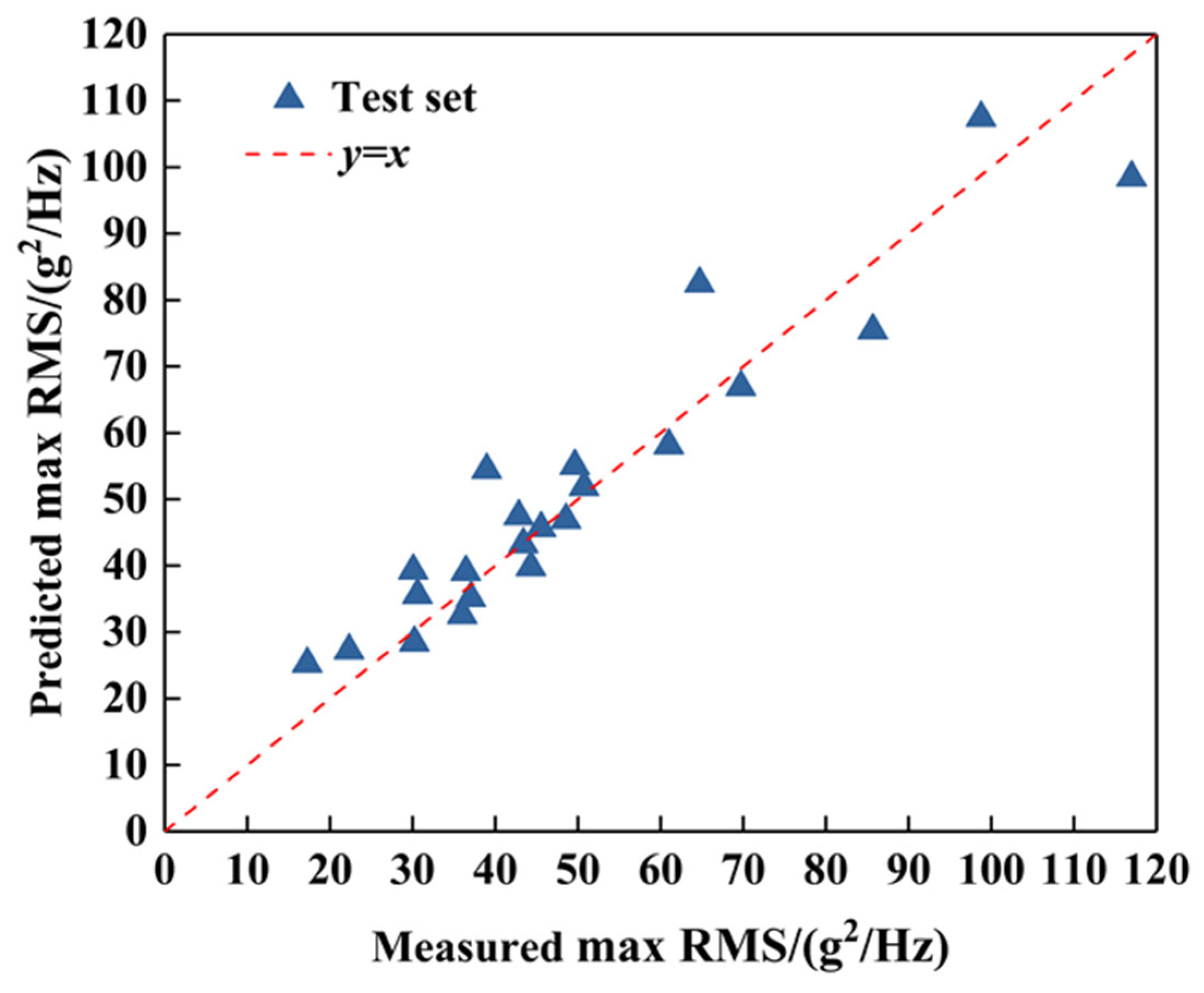
The SHAP method and partial dependence plot analysis show that the hydraulic testing oxidant injector pressure drop of the thrust chamber has a dominant effect on rocket engine vibration, and both excessively high and low injector pressure drops can cause an increasing trend in amplitude. Improvements were made to this type of engine based on data analysis results, reducing injector flow resistance and improving injector disk roughness. The subsequent test results showed that the average value of maximum RMS decreased by 3.02 g²/Hz, and the number of products with extremely large vibrations significantly decreased. The above results demonstrate the rationality of the method and its great potential in data mining for complex propellant systems.

References

1. Pan, T.; Zhang, S.; Li, F.; Chen, J.; Li, A. A meta network pruning framework for remaining useful life prediction of rocket engine bearings with temporal distribution discrepancy. Mech. Syst. Signal Process. 2023, 195, 110271. [Google Scholar] [CrossRef]
2. Li, F.; Chen, J.; Liu, Z.; Lv, H.; Wang, J.; Yuan, J.; Xiao, W. A soft-target difference scaling network via relational knowledge distillation for fault detection of liquid rocket engine under multi-source trouble-free samples. Reliab. Eng. Syst. Safe 2022, 228, 108759. [Google Scholar] [CrossRef]
3. Huang, Y.; Tao, J.; Zhao, J.; Sun, G.; Yin, K.; Zhai, J. Graph structure embedded with physical constraints-based information fusion network for interpretable fault diagnosis of aero-engine. Energy 2023, 283, 129120. [Google Scholar] [CrossRef]
4. Wang, J.; Wang, B.; Yang, H.; Sun, Z.; Zhou, K.; Zheng, X. Compressor geometric uncertainty quantification under conditions from near choke to near stall. Chin. J. Aeronaut. 2023, 36, 16–29. [Google Scholar] [CrossRef]
5. Cartocci, N.; Napolitano, M.R.; Costante, G.; Valigi, P.; Fravolini, M.L. Aircraft robust data-driven multiple sensor fault diagnosis based on optimality criteria. Mech. Syst. Signal Process. 2022, 170, 108668. [Google Scholar] [CrossRef]
6. Stanton, I.; Munir, K.; Ikram, A.; El-Bakry, M. Predictive maintenance analytics and implementation for aircraft: Challenges and opportunities. Syst. Eng. 2023, 26, 216–237. [Google Scholar] [CrossRef]
7. Xiaozhe, X.; Guangli, L.; Kaikai, Z.; Yao, X.; Siyuan, C.; Kai, C. Surrogate-based shape optimization and sensitivity analysis on the aerodynamic performance of HCW configuration. Aerosp. Sci. Technol. 2024, 152, 109347. [Google Scholar] [CrossRef]
8. Júnior, J.M.M.; Halila, G.L.; Kim, Y.; Khamvilai, T.; Vamvoudakis, K.G. Intelligent data-driven aerodynamic analysis and optimization of morphing configurations. Aerosp. Sci. Technol. 2022, 121, 107388. [Google Scholar] [CrossRef]
9. Du, B.; Shen, E.; Wu, J.; Guo, T.; Lu, Z.; Zhou, D. Aerodynamic Prediction and Design Optimization Using Multi-Fidelity Deep Neural Network. Aerospace 2025, 12, 292. [Google Scholar] [CrossRef]
10. Guan, P.; Huang, D.; He, M.; Zhou, B. Lung cancer gene expression database analysis incorporating prior knowledge with support vector machine-based classification method. J. Exp. Clin. Canc. Res. 2009, 28, 103. [Google Scholar] [CrossRef] [PubMed]
11. He, T.; Chen, Y.; Wang, L.; Cheng, H. An Expert-Knowledge-Based Graph Convolutional Network for Skeleton-Based Physical Rehabilitation Exercises Assessment. IEEE Trans. Neural Syst. Rehabil. Eng. 2024, 32, 1916–1925. [Google Scholar] [CrossRef] [PubMed]
12. Peng, H.; Yang, W. Knowledge Graph Construction Method for Commercial Aircraft Fault Diagnosis Based on Logic Diagram Model. Aerospace 2024, 11, 773. [Google Scholar] [CrossRef]
13. Karasu, S.; Altan, A.; Bekiros, S.; Ahmad, W. A new forecasting model with wrapper-based feature selection approach using multi-objective optimization technique for chaotic crude oil time series. Energy 2021, 212, 118750. [Google Scholar] [CrossRef]
14. Jenul, A.; Schrunner, S.; Pilz, J.; Tomic, O. A user-guided Bayesian framework for ensemble feature selection in life science applications (UBayFS). Mach. Learn. 2022, 111, 3897–3923. [Google Scholar] [CrossRef]
15. Liu, Y.; Zou, X.; Ma, S.; Avdeev, M.; Shi, S. Feature selection method reducing correlations among features by embedding domain knowledge. Acta Mater. 2022, 238, 118195. [Google Scholar] [CrossRef]
16. Liu, Y.; Wu, J.; Avdeev, M. Multi-Layer Feature Selection Incorporating Weighted Score-Based Expert Knowledge toward Modeling Materials with Targeted Properties. Adv. Theory Simul. 2020, 3, 1900215. [Google Scholar] [CrossRef]
17. Michelle, S.; Valentin, D. Family Rank: A graphical domain knowledge informed feature ranking algorithm. Bioinformatics 2021, 37, 3626–3631. [Google Scholar] [CrossRef] [PubMed]
18. Nanfack, G.; Temple, P.; Frenay, B. Learning Customised Decision Trees for Domain-knowledge Constraints. Pattern Recognit. 2023, 142, 109610. [Google Scholar] [CrossRef]
19. Fang, X.; Song, Q.; Wang, X.; Li, Z.; Ma, H.; Liu, Z. An intelligent tool wear monitoring model based on knowledge-data-driven physical-informed neural network for digital twin milling. Mech. Syst. Signal Process. 2025, 232, 112736. [Google Scholar] [CrossRef]
20. Lappas, Z.; Yannacopoulos, P.; Athanasios, N. A machine learning approach combining expert knowledge with genetic algorithms in feature selection for credit risk assessment. Appl. Soft Comput. 2021, 107, 107391. [Google Scholar] [CrossRef]
21. Sun, Y.N.; Qin, W.; Hu, J. A Causal Model-Inspired Automatic Feature-Selection Method for Developing Data-Driven Soft Sensors in Complex Industrial Processes. Engineering 2023, 3, 82–93. [Google Scholar] [CrossRef]
22. Xiong, J.W.; Fink, O.; Zhou, J. Controlled physics-informed data generation for deep learning-based remaining useful life prediction under unseen operation conditions. Mech. Syst. Signal Process. 2023, 197, 110359. [Google Scholar] [CrossRef]
23. Saltelli, A.; Annoni, P.; Azzini, I.; Campolongo, F.; Ratto, M.; Tarantola, S. Variance based sensitivity analysis of model output. Design and estimator for the total sensitivity index. Comput. Phys. Commun. 2010, 181, 259–270. [Google Scholar] [CrossRef]
24. Sobol, I.M. Global sensitivity indices for nonlinear mathematical models and their Monte Carlo estimates. Math. Comput. Simul. 2001, 55, 271–280. [Google Scholar] [CrossRef]
25. Huang, J.; Yan, X. Quality Relevant and Independent Two Block Monitoring Based on Mutual Information and KPCA. IEEE Trans. Ind. Electron. 2017, 64, 6518–6527. [Google Scholar] [CrossRef]
26. Alexander, S.; Anastasia, B.; Alexey, D. Efficient High-Order Interaction-Aware Feature Selection Based on Conditional Mutual Information. In Proceedings of the 30th International Conference on Neural Information Processing Systems, Barcelona, Spain, 5–10 December 2016. [Google Scholar]
27. Shang, C.; Li, M.; Feng, S.; Jiang, Q.; Fan, J. Feature selection via maximizing global information gain for text classification. Knowl-Based Syst. 2013, 54, 298–309. [Google Scholar] [CrossRef]
28. Bergstra, J.; Bardenet, R.; Bengio, Y.; Kégl, B. Algorithms for Hyper-Parameter Optimization. In Proceedings of the 25th International Conference on Neural Information Processing Systems, Lake Tahoe, NV, USA, 3–6 December 2011. [Google Scholar]
29. Lundberg, S.; Lee, S.I. A unified approach to interpreting model predictions. In Proceedings of the 31st International Conference on Neural Information Processing Systems, Montréal, QC, Canada, 3–8 December 2017. [Google Scholar]
30. Smith, M.; Alvarez, F. Identifying mortality factors from Machine Learning using Shapley values—A case of COVID19. Expert Syst. Appl. 2021, 176, 114832. [Google Scholar] [CrossRef] [PubMed]
31. Zhang, X.; Li, Y.; Ren, F.; Sha, Z.; Xu, P. Research on Virtual Prototype and Digital Test Method of Pump-Fed Propulsion System. Int. J. Aeronaut. Space Sci. 2025, 26, 815–833. [Google Scholar] [CrossRef]
Figure 1. Flow chart of explainable data mining of the liquid rocket engine.
Machines 13 00640 g001
Figure 2. Parameter correlation evaluation based on the weighted directed graph.
Machines 13 00640 g002
Figure 3. Flowchart of feature evaluation.
Machines 13 00640 g003
Figure 4. Flowchart of the two-stage optimization of the prediction model.
Machines 13 00640 g004
Figure 5. Rocket engine pressurization system.
Machines 13 00640 g005
Figure 6. Validation of the multi-criteria feature selection method using synthetic data set.
Machines 13 00640 g006
Figure 7. Df under different feature selection methods.
Machines 13 00640 g007
Figure 8. Changes of D ¯ mix D ¯ kn , D ¯ mix D ¯ ps , D ¯ mix min D ¯ ps , D ¯ kn , and D ¯ mix max D ¯ ps , D ¯ kn under different noise amplitudes (mean value).
Machines 13 00640 g008
Figure 9. Distributions of feature distances for three feature selection methods under different feature points.
Machines 13 00640 g009
Figure 10. The change of ri,min and ri,max with ωm.
Machines 13 00640 g010
Figure 11. The change in the high-performance region with ωm.
Machines 13 00640 g011
Figure 12. A certain rocket engine system on active service.
Machines 13 00640 g012
Figure 13. Frequency spectrum of engine vibration.
Machines 13 00640 g013
Figure 14. Feature evaluation metrics and feature rankings under different ωm.
Machines 13 00640 g014
Figure 15. The Spearman correlation coefficients of the feature rankings under ωm = 0.2~0.8 and under ωm = 0.
Machines 13 00640 g015
Figure 16. Top 10 features with the largest disparity between knowledge and model-based correlation and data-based correlation.
Machines 13 00640 g016
Figure 17. The impact of ωm and K on the distribution of RMSE.
Machines 13 00640 g017
Figure 18. Comparison between predicted values and measured values.
Machines 13 00640 g018
Figure 19. Path of the largest weight in the graph of knowledge and model.
Machines 13 00640 g019
Figure 20. Pearson correlation coefficient histogram of the 6 selected features.
Machines 13 00640 g020
Figure 21. SHAP values and SHAP scores of the selected features.
Machines 13 00640 g021
Figure 22. Partial dependency plots of the selected features.
Machines 13 00640 g022
Figure 23. The maximum RMS values before and after improvements: (a) Histogram of max RMS before improvements (a total of 124 engines). (b) Histogram of maximum RMS before improvements (a total of 40 engines). (c) Comparison of maximum RMS distribution before and after improvements.
Machines 13 00640 g023