Speed Sensorless Control for a Six-Phase Induction Machine Based on a Sliding Mode Observer

Abstract

This paper presents the application of a sliding mode observer for speed sensorless control of a six-phase induction machine. The use of nonlinear sliding mode techniques yields acceptable performance for both low- and high-speed motor operations over a wide speed range. The effectiveness and accuracy of the developed sensorless scheme are verified by experimental results, which demonstrate the system’s performance under various operating conditions. These results demonstrate the advantages of the proposal as a valid alternative to the conventional method, which uses a mechanical speed sensor for multiphase machines. Additionally, the sensorless approach can also serve as a redundant backup in the event of mechanical sensor failure, thereby increasing the reliability of the overall drive system.

1. Introduction

Multiphase induction machines have gained increasing attention as a promising alternative to conventional three-phase systems in a wide range of applications, offering advantages such as improved power distribution per phase, reduced torque ripple, and enhanced fault tolerance, features that are particularly desirable in electric traction systems [1,2]. Among the different topologies of multiphase induction machines, the asymmetrical Six-phase Induction Machine (SPIM) offers unique advantages, such as suppression of torque harmonics and increased fault tolerance due to the isolated neutral configuration. These characteristics make SPIMs particularly well-suited for applications that demand high reliability under fault conditions.

The adoption of multiphase machines has been accompanied by advances in control strategies, which typically require rotor position and/or speed information. This information is typically acquired using mechanical sensors mounted on the motor shaft, which introduces potential drawbacks, including reduced overall system reliability due to susceptibility to vibrations, limited operational performance, increased installation complexity, and the additional cost associated with the sensors themselves.

Given the constraints of sensor-based systems, speed sensorless control strategies are increasingly recognized as an effective approach to overcoming these limitations, offering advantages such as reduced hardware complexity, lower cost, more compact system design, elimination of sensor wiring, and improved noise immunity. Furthermore, they have become increasingly important in applications involving harsh operating environments. Even in systems equipped with mechanical speed sensors, sensorless estimation can provide redundancy, allowing continued operation in the event of sensor failure [3,4,5]. These combined benefits have driven significant advancements in the development of speed estimation methods for multiphase machines.

Despite these advantages, one significant challenge in sensorless control is the variation of motor parameters, which are strongly influenced by changes in ambient temperature. These parameter drifts introduce additional complexity in the control system design and increase the computational demands of the estimation algorithms. To cope with these issues, advanced estimation techniques, particularly observer-based approaches, have shown the potential to improve performance, provided they are robust enough to handle parameter deviations across a broad range of operating speeds [6].

Within this context, various sensorless speed estimation techniques have been proposed. Among them, the Model Reference Adaptive System (MRAS) is widely recognized for its reliable performance across a wide speed range. However, MRAS-based approaches tend to be highly sensitive to parameter variations at low speeds, which limits their accuracy. Additionally, their implementation is often complicated by the need to tune adaptation gains for PI controllers [6]. Another standard method is the Extended Kalman Filter (EKF), a stochastic observer capable of accurate estimation under certain conditions. Nevertheless, its effectiveness is hindered by strong sensitivity to noise characteristics, a complex design process, and high computational cost [7].

As a robust alternative, Sliding Mode Observers (SMOs) have emerged as a promising solution, offering strong robustness against parameter uncertainties and external disturbances [8,9,10]. A notable example is the SMO proposed by [11] for three-phase induction machines, which achieves accurate speed estimation across the entire speed range using only a single observer gain, thereby simplifying implementation. Nevertheless, the practical deployment of SPIMs introduces several challenges, such as increased system complexity and the necessity for more sophisticated control and estimation models. Likewise, SMO-based observers, despite their robustness, can suffer from chattering and require careful gain tuning.

Recent contributions have further advanced sensorless strategies designed explicitly for SPIMs, particularly under challenging operating conditions such as low speeds, parameter variations, and fault scenarios. In [12], an MRAS-based rotor time constant estimator is proposed, combined with an adaptive observer that enables simultaneous estimation of the rotor speed and time constant, thus enhancing robustness in sensorless Indirect Rotor Field-Oriented Control (IFOC) systems. This method is particularly relevant for SPIMs, where parameter mismatches significantly degrade control performance. On the other hand, in [13] is demonstrates that EKF can be successfully used in sensorless frameworks to estimate not only rotor speed but also parameters such as resistance, contributing to efficient operation across the entire speed range. The EKF-based estimation is shown to improve loss model control, making it a viable option for high-efficiency sensorless control. Additionally, in [14], which is related to fault-tolerant applications, an SMO adapted to identify rotor flux and speed even under open-circuit faults is presented. The SMO is integrated with harmonic suppression strategies, offering strong robustness and maintaining control reliability under both healthy and faulty conditions. These developments highlight the growing interest in hybrid estimation and control strategies, motivating the proposed integration of SMO within an IRFOC-based sensorless control framework for asymmetrical SPIMs, as also reviewed comprehensively in [15].

The adoption of SMOs in sensorless control of induction machines has gained significant attention due to their robust performance. SMOs maintain precise flux and speed estimations even in the face of parameter uncertainties and external disturbances, making them especially beneficial for SPIMs that require effective decoupling of multiple subspaces. They also offer rapid dynamic responses and reduce reliance on accurate machine parameters compared to model-based estimators, such as MRAS and EKF. However, challenges exist, such as the chattering phenomenon from the discontinuous nature of the sliding-mode control law, which can excite unmodeled high-frequency dynamics or amplify noise. Performance may also degrade in the presence of measurement noise, necessitating careful tuning of observer gains to balance convergence speed and noise sensitivity. Despite these issues, SMOs remain a captivating option for robust sensorless control.

This work extends the sensorless control strategy initially proposed in [11] to SPIM, thereby broadening its applicability within the field of multiphase drive systems. Although multiphase machines offer significant advantages, directly extrapolating control techniques from three-phase systems poses challenges due to increased system dimensionality, complex coupling between harmonics, and the need for adapted mathematical modeling. The main contribution of this work is the proposal and experimental validation of a sensorless control scheme based on SMO applied to SPIMs within an IRFOC scheme under various operating conditions, maintaining its simplicity and low computational cost. This approach not only demonstrates robust performance but can also, due to its modular structure and independence from the torque and flux controllers, be readily extended to other advanced control strategies, thereby opening new possibilities for applications in multiphase systems.

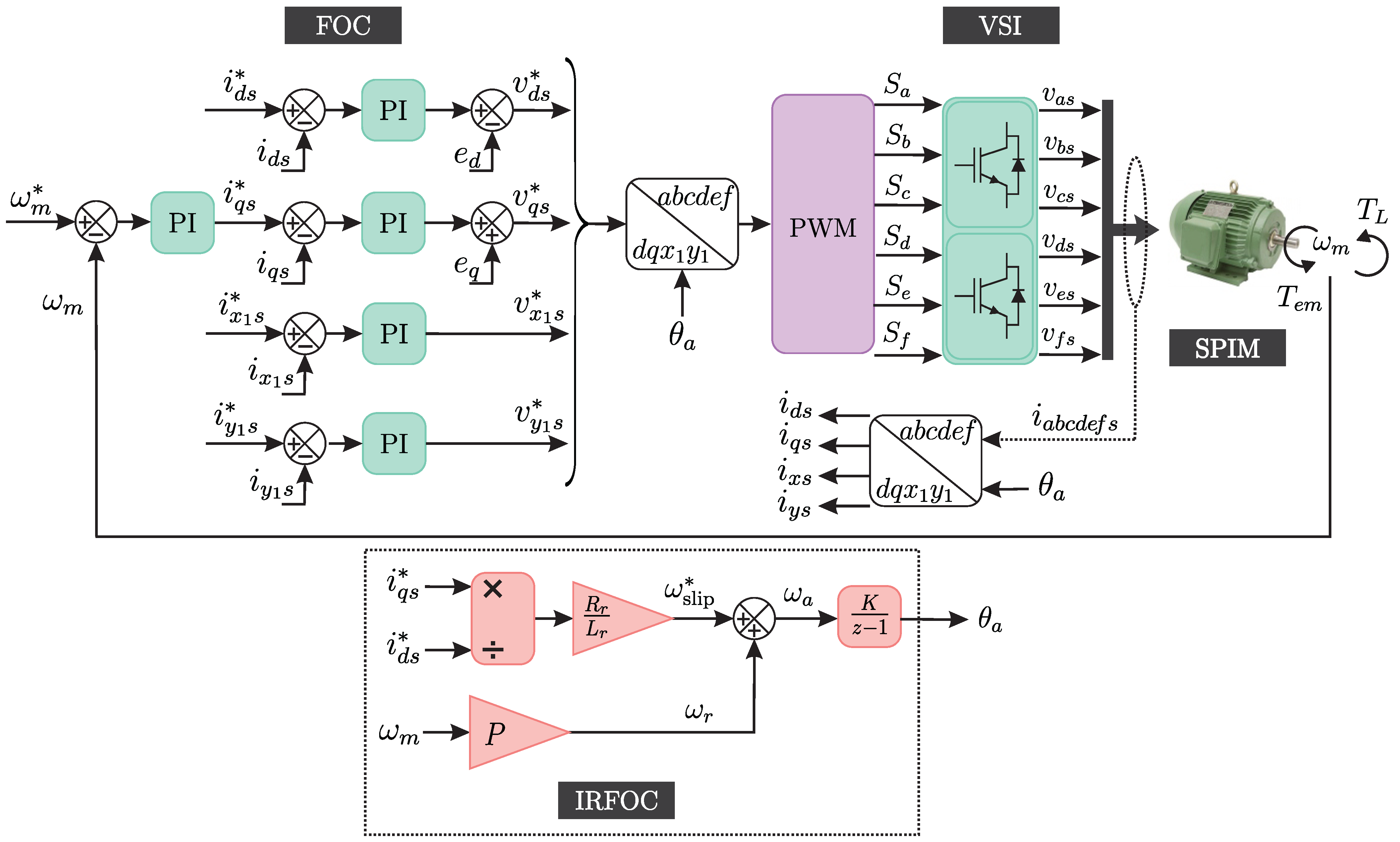
The remainder of this paper is organized as follows: Section 2 presents the mathematical model of the system. The outer speed control and inner current control, utilizing the sensorless technique, are presented in Section 3. Simulation and experimental validation of the proposal in transient and steady-state conditions are developed in Section 4. Section 5 discusses the obtained results using figures of merit. Finally, Section 6 presents the conclusions.

2. Mathematical SPIM Model

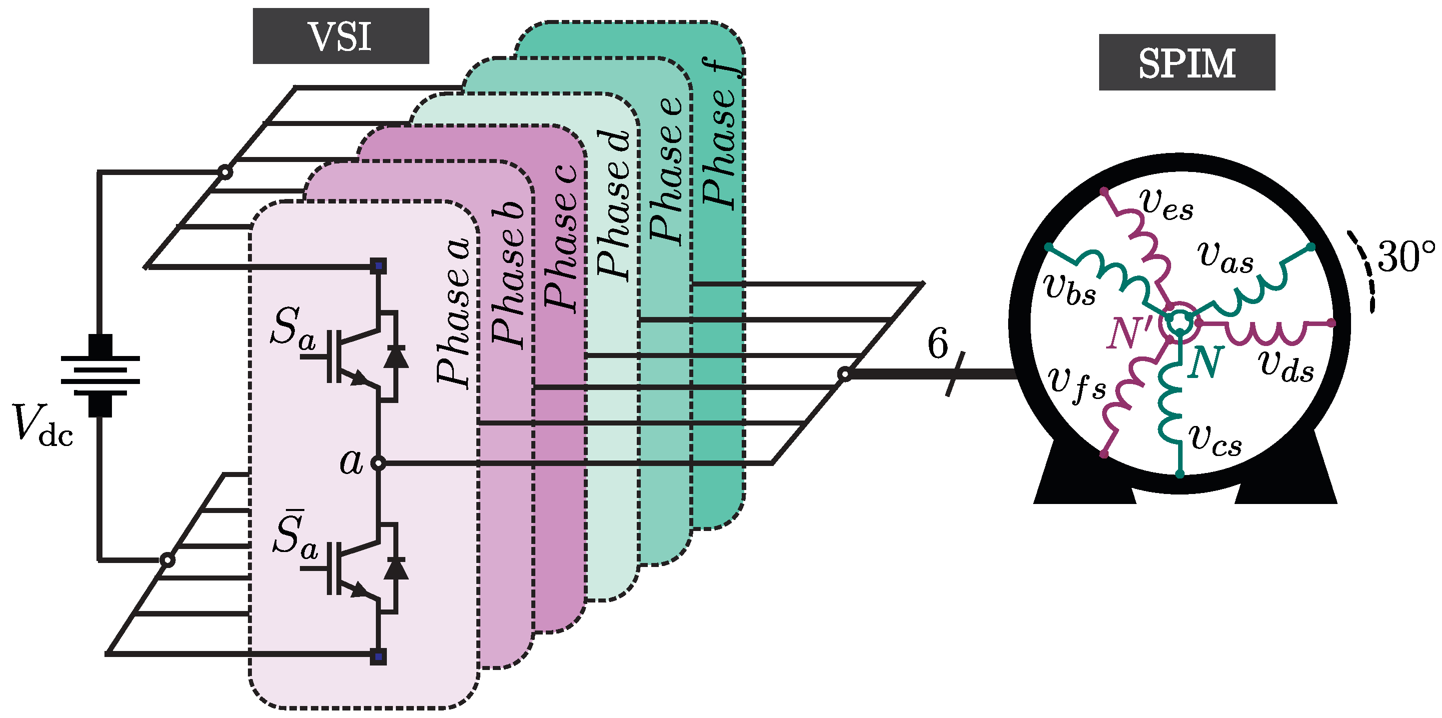
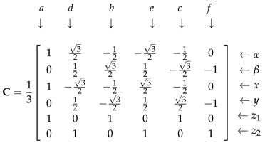
The SPIM under consideration is asymmetrical, featuring a ${30}^{\circ }$ phase shift between its two three-phase winding sets, as shown in Figure 1. The machine model is initially described by a set of differential equations with time-varying coefficients, traditionally formulated in terms of phase variables ($a,d,b,e,c,f$). Among the various reference frames described in the literature, Vector Space Decomposition (VSD) remains one of the most commonly adopted approaches [16,17]. By applying the Clarke transformation to both stator and rotor phase variables, according to the amplitude-invariant criterion, as shown in Equation (1), a transformed mathematical model with constant coefficients is derived [18]. This transformation allows the final SPIM equations to be expressed in the stationary reference frame, which not only simplifies the mathematical representation but also facilitates the implementation of advanced control strategies.

(1)

$${\left[f_{\alpha }{f}_{\beta }{f}_x{f}_y{f}_{z1}{f}_{z2}\right]}^T=\left[\mathbf{C}\right]{\left[f_a{f}_d{f}_b{f}_e{f}_c{f}_f\right]}^T$$

(2)

where ${\left[f_{\alpha }{f}_{\beta }{f}_x{f}_y{f}_{z1}{f}_{z2}\right]}^T$ is the column vector representing the electrical quantities, voltage, current, or flux, corresponding to both the stator and the rotor after the transformation, whereas ${\left[f_a{f}_d{f}_b{f}_e{f}_c{f}_f\right]}^T$ denotes the column vector expressed in terms of the phase variables in a predefined order.

As a result, the original machine system is decomposed into three bi-dimensional subspaces, defined as follows: the ($\alpha$-$\beta$) subspace contributes to the air-gap flux and electromagnetic torque, representing the fundamental supply component along with harmonics of order $12n\pm 1$ ($n=1,2,3,\dots$); the (x-y) subspace is associated with copper losses and includes all supply harmonics of order $6n\pm 1$; and the ($z_1$- $z_2$) subspace corresponds to zero-sequence harmonic components, whose circulation is inhibited due to the isolated neutral point configuration [16]. Accordingly, the machine model can be expressed in terms of the following equations:

$$\begin{array}{cc}\hfill v_{\alpha s}& =R_s{i}_{\alpha s}+{\displaystyle \frac{d}{dt}}{\psi }_{\alpha s}=R_s{i}_{\alpha s}+L_s{\displaystyle \frac{d}{dt}}{i}_{\alpha s}+M{\displaystyle \frac{d}{dt}}{i}_{\alpha r}\hfill \end{array}$$

(3)

$$\begin{array}{cc}\hfill v_{\beta s}& =R_s{i}_{\beta s}+{\displaystyle \frac{d}{dt}}{\psi }_{\beta s}=R_s{i}_{\beta s}+L_s{\displaystyle \frac{d}{dt}}{i}_{\beta s}+M{\displaystyle \frac{d}{dt}}{i}_{\beta r}\hfill \end{array}$$

(4)

$$\begin{array}{cc}\hfill v_{\alpha r}=0& =R_r{i}_{\alpha r}+{\displaystyle \frac{d}{dt}}{\psi }_{\alpha r}+{\omega }_r{\psi }_{\beta r}=R_r{i}_{\alpha r}+L_r{\displaystyle \frac{d}{dt}}{i}_{\alpha r}+M{\displaystyle \frac{d}{dt}}{i}_{\alpha s}+{\omega }_r(M{i}_{\beta s}+L_r{i}_{\beta r})\hfill \end{array}$$

(5)

$$\begin{array}{cc}\hfill v_{\beta r}=0& =R_r{i}_{\beta r}+{\displaystyle \frac{d}{dt}}{\psi }_{\beta r}-{\omega }_r{\psi }_{\alpha r}=R_r{i}_{\beta r}+L_r{\displaystyle \frac{d}{dt}}{i}_{\beta r}+M{\displaystyle \frac{d}{dt}}{i}_{\beta s}-{\omega }_r(M{i}_{\alpha s}+L_r{i}_{\alpha r})\hfill \end{array}$$

(6)

$$\begin{array}{cc}\hfill v_{xs}& =R_s{i}_{xs}+{\displaystyle \frac{d}{dt}}{\psi }_{xs}=R_s{i}_{xs}+L_{ls}{\displaystyle \frac{d}{dt}}{i}_{xs}\hfill \end{array}$$

(7)

$$\begin{array}{cc}\hfill v_{ys}& =R_s{i}_{ys}+{\displaystyle \frac{d}{dt}}{\psi }_{ys}=R_s{i}_{ys}+L_{ls}{\displaystyle \frac{d}{dt}}{i}_{ys}\hfill \end{array}$$

(8)

$$\begin{array}{cc}\hfill v_{z_{1}s}& =R_s{i}_{z_{1}s}+{\displaystyle \frac{d}{dt}}{\psi }_{z_{1}s}=R_s{i}_{z_{1}s}+L_{ls}{\displaystyle \frac{d}{dt}}{i}_{z_{1}s}\hfill \end{array}$$

(9)

$$\begin{array}{cc}\hfill v_{z_{2}s}& =R_s{i}_{z_{2}s}+{\displaystyle \frac{d}{dt}}{\psi }_{z_{2}s}=R_s{i}_{z_{2}s}+L_{ls}{\displaystyle \frac{d}{dt}}{i}_{z_{2}s}\hfill \end{array}$$

(10)

where mutual inductance $M=3L_m$, $L_s=L_{ls}+M$, $L_r=L_{lr}+M$ and ${\omega }_r$ is the electrical speed of the rotor. On the other hand, the indices s, and r denote the stator and rotor variables, respectively, while the subscripts l and m refer to the leakage and magnetization inductance, respectively.

The expressions for stator and rotor flux are given by:

$$\begin{array}{cc}{\psi }_{\alpha s}=L_s{i}_{\alpha s}+M{i}_{\alpha r},\hfill & {\psi }_{\beta s}=L_s{i}_{\beta s}+M{i}_{\beta r},\hfill \\ {\psi }_{\alpha r}=L_r{i}_{\alpha r}+M{i}_{\alpha s},\hfill & {\psi }_{\beta r}=L_r{i}_{\beta r}+M{i}_{\beta s},\hfill \\ {\psi }_{xs}=L_{ls}{i}_{xs},\hfill & {\psi }_{ys}=L_{ls}{i}_{ys},\hfill \\ {\psi }_{z_{1}s}=L_{ls}{i}_{z_{1}s},\hfill & {\psi }_{z_{2}s}=L_{ls}{i}_{z_{2}s}.\hfill \end{array}$$

(11)

Finally, the expression for the electromagnetic torque $T_{em}$, of the SPIM is given as follows:

$$T_{em}={\displaystyle \frac{6}{2}}PM(i_{\alpha r}{i}_{\beta s}-i_{\beta r}{i}_{\alpha s}),$$

(12)

where P represents the number of magnetic pole pairs.

The equation relating the torque and mechanical parameters of the machine with respect to the mechanical speed is given by:

$$T_{em}-T_L=J{\displaystyle \frac{d}{dt}}{\omega }_m+B{\omega }_m,$$

(13)

where $T_L$ is the torque of the mechanical load, J is the inertia coefficient, B is the mechanical friction coefficient, and ${\omega }_m$ is the mechanical speed of the rotor. The latter is commonly represented as a function of the electrical speed ${\omega }_r$, being:

$${\omega }_m={\displaystyle \frac{{\omega }_r}{P}}.$$

(14)

Then, rewriting the mechanical equation, we obtain:

$$T_{em}-T_L={\displaystyle \frac{J}{P}}{\displaystyle \frac{d}{dt}}{\omega }_r+{\displaystyle \frac{B}{P}}{\omega }_r.$$

(15)

3. Proposed Speed Sensorless Control

Closed-loop control is essential for achieving high-performance operation and typically relies on feedback from measurements of stator current and rotor speed. When an estimated value replaces the actual speed sensor, the drive is considered sensorless; however, the overall control structure remains fundamentally the same as in its sensored counterpart. The main goal of the control system is to process these input signals and determine the appropriate switching pattern for the Voltage Source Inverter (VSI) at each sampling interval. While some advanced strategies, such as model predictive control, can compute the optimal switching states directly, it is more common practice to employ a modulation stage. In such cases, the control algorithm generates phase voltage references, which are then used as inputs for the Pulse Width Modulation (PWM) block. This is the case for Field-Oriented Control (FOC), which will be briefly described in the following section.

3.1. Field Oriented Control

Indirect Rotor Field-Oriented Control (IRFOC) is a widely adopted vector control method valued for its simplicity in design and ease of implementation. Initially developed for conventional three-phase induction machines, IRFOC has been successfully extended to multiphase systems, such as the SPIM considered in this study. This technique enables precise regulation of both torque and speed by controlling the electromagnetic state of the machine [17,19].

In the IRFOC approach, the stator currents are transformed from the stationary ($\alpha$-$\beta$) frame to a synchronously rotating (d–q) reference frame using the Park transformation. This coordinate transformation facilitates the alignment of the direct axis (d-axis) with the rotor flux vector, effectively decoupling the control of magnetic flux from torque production. As a result, the d-axis current component primarily influences the stator flux, while the quadrature-axis (q-axis) component is responsible for generating the electromagnetic torque, enabling independent regulation of both within the control scheme [20]. The Park matrix is typically expressed as:

$$\left[D\right]=\left[\begin{array}{cc}cos\left({\theta }_a\right)& sin\left({\theta }_a\right)\\ -sin\left({\theta }_a\right)& cos\left({\theta }_a\right)\end{array}\right],$$

(16)

$${\left[i_{ds}{i}_{qs}\right]}^T=\left[\mathbf{D}\right]{\left[i_{\alpha s}{i}_{\beta s}\right]}^T,$$

(17)

$${\left[i_{x_{1}s}{i}_{y_{1}s}\right]}^T=\left[\mathbf{D}\right]{\left[i_{xs}{i}_{ys}\right]}^T,$$

(18)

where ${\theta }_a$ corresponds to the angular position of the rotating reference frame, which is determined based on the measured (or estimated) mechanical speed and the estimated slip frequency ${\omega }_{\mathrm{slip}}$. The calculation of ${\omega }_{\mathrm{slip}}$ makes use of the reference values of the stator currents in the (d–q) coordinate frame, $i_{ds}^{*}$ and $i_{qs}^{*}$, along with rotor electrical parameters $R_r$ and $L_r$. The complete structure of the IRFOC is illustrated in Figure 2.

A standard IRFOC scheme presents two different control loops. The mechanical speed regulation is achieved via an outer control loop, which employs a PI regulator equipped with output limiting and an anti-windup mechanism, as detailed in [21]. The selection of a PI structure is based on its ease of implementation and robust performance under varying conditions. This controller is responsible for generating the time-varying reference for the q-axis component of the stator current, $i_{qs}^{*}$. The control law governing the speed loop is expressed as:

$$i_{qs}^{*}=K_p({\omega }_m^{*}-{\omega }_m)+{\displaystyle \frac{K_i({\omega }_m^{*}-{\omega }_m)}{z-1}},$$

(19)

where $K_p$ and $K_i$ correspond to the proportional and integral gains of the controller. This formulation assumes the use of an encoder to measure the mechanical speed ${\omega }_m$ directly. In the case of sensorless operation, the estimated speed ${\hat{\omega }}_m$ is used instead, and it is compared with the reference speed ${\omega }_m^{*}$ within the PI controller to regulate $i_{qs}^{*}$.

In the inner current control loop, multiple current regulators are implemented to achieve accurate flux and torque control while maintaining acceptable levels of harmonic distortion, as shown in Equations (20) and (21). The reference for the direct-axis (d-axis) current is fixed at its nominal value to guarantee proper magnetization of the machine. Regarding the dynamic behavior of the drive, the speed response is predominantly influenced by the quadrature-axis (q-axis) current, owing to its direct relationship with electromagnetic torque generation. Additionally, the reference values of the ($i_{x_{1}s}^{*}$-$i_{y_{1}s}^{*}$) current components are set to zero to reduce stator copper losses, taking advantage of the isolated neutrals configuration in the proposed SPIM.

$$\begin{array}{cc}\hfill v_{ds}^{*}=& (i_{ds}^{*}-i_{ds})(K_p+{\displaystyle \frac{K_i}{z-1}})-i_{qs}({\omega }_r+{\omega }_{\mathrm{slip}})L_s(1-{\displaystyle \frac{M^2}{L_s{L}_r}}),\hfill \end{array}$$

(20)

$$\begin{array}{cc}\hfill v_{qs}^{*}=& (i_{qs}^{*}-i_{qs})(K_p+{\displaystyle \frac{K_i}{z-1}})+i_{ds}({\omega }_r+{\omega }_{\mathrm{slip}})L_s.\hfill \end{array}$$

(21)

The output of this cascaded control scheme consists of the reference values for the (d-q) and ($x_1$-$y_1$) voltage components. Following this, a separate modulation stage is required to determine the switching states and their corresponding duty cycles, enabling the generation of the reference phase voltages. This study considers the use of the Carrier-Based Pulse Width Modulation (CB-PWM) technique, as it is the most widely adopted due to its ease of implementation on Digital Signal Processors (DSPs) [22]. A triangular carrier signal is employed, owing to its optimal performance in harmonic mitigation.

3.2. Sliding Mode Observer

The following state equations are used for the proposed observer:

$$\begin{array}{cc}\hfill {\displaystyle \frac{d}{dt}}{\psi }_{\alpha r}& =-a_5{\psi }_{\alpha r}-{\omega }_r{\psi }_{\beta r}+a_4{i}_{\alpha s},\hfill \end{array}$$

(22)

$$\begin{array}{cc}\hfill {\displaystyle \frac{d}{dt}}{\psi }_{\beta r}& =-a_5{\psi }_{\beta r}+{\omega }_r{\psi }_{\alpha r}+a_4{i}_{\beta s},\hfill \end{array}$$

(23)

$$\begin{array}{cc}\hfill {\displaystyle \frac{d}{dt}}{i}_{\alpha s}& =a_2{\psi }_{\alpha r}+a_3{\omega }_r{\psi }_{\beta r}-a_1{i}_{\alpha s}+a_6{v}_{\alpha s},\hfill \end{array}$$

(24)

$$\begin{array}{cc}\hfill {\displaystyle \frac{d}{dt}}{i}_{\beta s}& =a_2{\psi }_{\beta r}-a_3{\omega }_r{\psi }_{\alpha r}-a_1{i}_{\beta s}+a_6{v}_{\beta s}.\hfill \end{array}$$

(25)

The corresponding coefficients are given by:

$$\begin{array}{ccc}{a}_1={\displaystyle \frac{R_s}{\sigma L_s}}+{\displaystyle \frac{M^2}{\sigma L_s{L}_r{\tau }_r}},\hfill & a_2={\displaystyle \frac{M}{\sigma L_s{L}_r{\tau }_r}},\hfill & a_3={\displaystyle \frac{M}{\sigma L_s{L}_r}},\hfill \\ a_4={\displaystyle \frac{M}{{\tau }_r}},\hfill & a_5={\displaystyle \frac{1}{{\tau }_r}},\hfill & a_6={\displaystyle \frac{1}{\sigma L_s}}\hfill \end{array}$$

(26)

where ${\tau }_r={\displaystyle \frac{L_r}{R_r}}$ and $\sigma =1-{\displaystyle \frac{M^2}{L_s{L}_r}}$.

Sensorless control requires the simultaneous observation of both rotor flux and rotor speed, and the following equations must be defined:

$$\begin{array}{cc}\hfill {\displaystyle \frac{d}{dt}}{\hat{\psi }}_{\alpha r}& =-a_5{\hat{\psi }}_{\alpha r}-{\hat{\omega }}_r{\hat{\psi }}_{\beta r}+a_4{i}_{\alpha s},\hfill \end{array}$$

(27)

$$\begin{array}{cc}\hfill {\displaystyle \frac{d}{dt}}{\hat{\psi }}_{\beta r}& =-a_5{\hat{\psi }}_{\beta r}+{\hat{\omega }}_r{\hat{\psi }}_{\alpha r}+a_4{i}_{\beta s},\hfill \end{array}$$

(28)

$$\begin{array}{cc}\hfill {\displaystyle \frac{d}{dt}}{\hat{i}}_{\alpha s}& =a_2{\hat{\psi }}_{\alpha r}+a_3{\hat{\omega }}_r{\hat{\psi }}_{\beta r}-a_1{\hat{i}}_{\alpha s}+a_6{v}_{\alpha s},\hfill \end{array}$$

(29)

$$\begin{array}{cc}\hfill {\displaystyle \frac{d}{dt}}{\hat{i}}_{\beta s}& =a_2{\hat{\psi }}_{\beta r}-a_3{\hat{\omega }}_r{\hat{\psi }}_{\alpha r}-a_1{\hat{i}}_{\beta s}+a_6{v}_{\beta s},\hfill \end{array}$$

(30)

where ${\hat{\psi }}_{\alpha r}$ and ${\hat{\psi }}_{\beta r}$ are the estimated rotor fluxes components, ${\hat{i}}_{\alpha s}$ and ${\hat{i}}_{\beta s}$ are the estimated stator currents components, ${\hat{\omega }}_r$ is the estimated electrical rotor speed, and $i_{\alpha s}$ and $i_{\beta s}$ are the measured stator currents components.

In order to express the mismatch between the measured and estimated variables, the following expressions are used:

$$\begin{array}{cc}{\overline{i}}_{\alpha s}={\hat{i}}_{\alpha s}-i_{\alpha s},\hfill & {\overline{i}}_{\beta s}={\hat{i}}_{\beta s}-i_{\beta s},\hfill \\ {\overline{\psi }}_{\alpha s}={\hat{\psi }}_{\alpha s}-{\psi }_{\alpha s},\hfill & {\overline{\psi }}_{\beta s}={\hat{\psi }}_{\beta s}-{\psi }_{\beta s},\hfill \\ {\overline{\omega }}_r={\hat{\omega }}_r-{\omega }_r\hfill & \hfill \end{array}$$

(31)

$$\begin{array}{cc}\hfill {\displaystyle \frac{d}{dt}}{\overline{i}}_{\alpha s}& =-a_1{\overline{i}}_{\alpha s}+a_2{\overline{\psi }}_{\alpha r}+a_3{\omega }_r{\overline{\psi }}_{\beta r}+a_3{\overline{\omega }}_r{\hat{\psi }}_{\beta r},\hfill \end{array}$$

(32)

$$\begin{array}{cc}\hfill {\displaystyle \frac{d}{dt}}{\overline{i}}_{\beta s}& =-a_1{\overline{i}}_{\beta s}+a_2{\overline{\psi }}_{\beta r}-a_3{\omega }_r{\overline{\psi }}_{\alpha r}-a_3{\overline{\omega }}_r{\hat{\psi }}_{\alpha r},\hfill \end{array}$$

(33)

$$\begin{array}{cc}\hfill {\displaystyle \frac{d}{dt}}{\overline{\psi }}_{\alpha r}& =-a_5{\overline{\psi }}_{\alpha r}-{\overline{\omega }}_r{\hat{\psi }}_{\beta r}-{\omega }_r{\overline{\psi }}_{\beta r},\hfill \end{array}$$

(34)

$$\begin{array}{cc}\hfill {\displaystyle \frac{d}{dt}}{\overline{\psi }}_{\beta r}& =-a_5{\overline{\psi }}_{\beta r}+{\overline{\omega }}_r{\hat{\psi }}_{\alpha r}-{\omega }_r{\overline{\psi }}_{\alpha r}.\hfill \end{array}$$

(35)

A block diagram of the proposed SMO is shown in Figure 3. The SMO uses the estimated speed to improve the observation of stator currents and rotor fluxes. This correction is based on a sliding surface that combines the stator current measurements with the rotor flux estimation and a low pass filter. Based on Lyapunov theory [11,23,24], a discontinuous function is derived that enables the estimation of rotor speed from the applied stator voltages $v_{\alpha s}$ and $v_{\beta s}$ and the measured stator currents $i_{\alpha s}$ and $i_{\beta s}$.

3.2.1. Stability of the Current Estimation Error

A positive Lyapunov function is defined as:

$$\begin{array}{c}\hfill I={\displaystyle \frac{1}{2}}({\overline{i}}_{\alpha s}^2+{\overline{i}}_{\beta s}^2).\end{array}$$

(36)

The time derivative is obtained from the error dynamics using Equations (32) and (33):

$$\begin{array}{cc}\hfill {\displaystyle \frac{d}{dt}}I& ={\displaystyle \frac{d}{dt}}{\overline{i}}_{\alpha s}{\overline{i}}_{\alpha s}+{\displaystyle \frac{d}{dt}}{\overline{i}}_{\beta s}{\overline{i}}_{\beta s},\hfill \\ \hfill & =-2a_{1}I-a_3{\omega }_r({\hat{S}}_n-S_n)-a_3{\overline{\omega }}_r{\hat{S}}_n+a_2{S}_c,\hfill \end{array}$$

(37)

where:

$$\begin{array}{cc}{\hat{S}}_n={\overline{i}}_{\beta s}{\hat{\psi }}_{\alpha r}-{\overline{i}}_{\alpha s}{\hat{\psi }}_{\beta r},\hfill & {\hat{S}}_n-S_n={\overline{i}}_{\beta s}{\overline{\psi }}_{\alpha r}-{\overline{i}}_{\alpha s}{\overline{\psi }}_{\beta r},\hfill \\ S_n={\overline{i}}_{\beta s}{\psi }_{\alpha r}-{\overline{i}}_{\alpha s}{\psi }_{\beta r},\hfill & \\ S_c={\overline{i}}_{\alpha s}{\overline{\psi }}_{\alpha r}+{\overline{i}}_{\beta s}{\overline{\psi }}_{\beta r}.\hfill \end{array}$$

(38)

Stability of the current estimation error is ensured if the conditions ${\displaystyle \frac{d}{dt}}I<0$ and $I\ge 0$ are true and can be written as follows:

$$\begin{array}{cc}\hfill 0& >-2a_{1}I-a_3{\omega }_r({\hat{S}}_n-S_n)-a_3{\overline{\omega }}_r{\hat{S}}_n+a_2{S}_c\hfill \\ \hfill {\omega }_r({\hat{S}}_n-S_n)+{\overline{\omega }}_r{\hat{S}}_n& >-2{\displaystyle \frac{a_1}{a_3}}I+{\displaystyle \frac{a_2}{a_3}}{S}_c.\hfill \end{array}$$

(39)

The control law is defined as:

$$\begin{array}{c}\hfill {\hat{\omega }}_r=K_s\mathrm{sgn}\left({\hat{S}}_n\right),\end{array}$$

(40)

where $K_s$ is a positive constant and $\mathrm{sgn}\left({\hat{S}}_n\right)$ is the sgn function of the sliding surface, which is defined as follows:

$$\mathrm{sgn}\left({\hat{S}}_n\right)=\left\{\begin{array}{cc}1,& \mathrm{for}{\hat{S}}_n>0,\\ 0,& \mathrm{for}{\hat{S}}_n=0,\\ -1,& \mathrm{for}{\hat{S}}_n<0.\end{array}\right.$$

(41)

The sufficient condition is therefore:

$$\begin{array}{cc}\hfill K_s|{\hat{S}}_n|& >{\omega }_r|S_n|-2{\displaystyle \frac{a_1}{a_3}}I+{\displaystyle \frac{a_2}{a_3}}|S_c|.\hfill \end{array}$$

(42)

Under these conditions, the current estimation errors converge to zero, and the system enters the sliding regime.

3.2.2. Stability of the Rotor Flux Estimation Error

Once the system reaches the sliding mode, ${\hat{S}}_n=0$ and ${\displaystyle \frac{d}{dt}}{\hat{S}}_n=0$, the current estimation errors converge to zero. This results in the following expression:

$$\begin{array}{c}\hfill {\displaystyle \frac{d}{dt}}{\hat{S}}_n=a_2({\overline{\psi }}_{\beta r}{\hat{\psi }}_{\alpha r}-{\overline{\psi }}_{\alpha r}{\hat{\psi }}_{\beta r})-a_3{\hat{\omega }}_r({\overline{\psi }}_{\alpha s}^2+{\overline{\psi }}_{\beta s}^2)+a_3{\omega }_r({\psi }_{\alpha r}{\hat{\psi }}_{\alpha r}+{\psi }_{\beta r}{\hat{\psi }}_{\beta r})=0.\end{array}$$

(43)

Rearranging the previous equation with respect to ${\hat{\omega }}_r$ yields the following result:

$$\begin{array}{c}\hfill {\hat{\omega }}_r={\omega }_r{\displaystyle \frac{{\psi }_{\alpha r}{\hat{\psi }}_{\alpha r}+{\psi }_{\beta r}{\hat{\psi }}_{\beta r}}{{\hat{\psi }}_{\alpha r}^2+{\hat{\psi }}_{\beta r}^2}}+a_5{\displaystyle \frac{{\overline{\psi }}_{\beta r}{\hat{\psi }}_{\alpha r}-{\overline{\psi }}_{\alpha r}{\hat{\psi }}_{qr}}{{\hat{\psi }}_{\alpha r}^2+{\hat{\psi }}_{\beta r}^2}}.\end{array}$$

(44)

Substituting Equation (44) into the rotor flux mismatch dynamics given by Equations (34) and (35) yields the following linear system:

$$\left[\begin{array}{c}{\displaystyle \frac{d}{dt}}{\overline{\psi }}_{\alpha r}\\ {\displaystyle \frac{d}{dt}}{\overline{\psi }}_{\beta r}\end{array}\right]=\left[\begin{array}{cc}{\displaystyle \frac{-a_5{\hat{\psi }}_{\alpha r}^2+{\omega }_r{\hat{\psi }}_{\alpha r}{\hat{\psi }}_{\beta r}}{{\hat{\psi }}_{\alpha r}^2+{\hat{\psi }}_{\beta r}^2}}& {\displaystyle \frac{-{\omega }_r{\hat{\psi }}_{\alpha r}^2-a_5{\hat{\psi }}_{\alpha r}{\hat{\psi }}_{\beta r}}{{\hat{\psi }}_{\alpha r}^2+{\hat{\psi }}_{\beta r}^2}}\\ {\displaystyle \frac{{\omega }_r{\hat{\psi }}_{\beta r}^2-a_5{\hat{\psi }}_{\alpha r}{\hat{\psi }}_{\beta r}}{{\hat{\psi }}_{\alpha r}^2+{\hat{\psi }}_{\beta r}^2}}& {\displaystyle \frac{-a_5{\hat{\psi }}_{\beta r}^2-{\omega }_r{\hat{\psi }}_{\alpha r}{\hat{\psi }}_{\beta r}}{{\hat{\psi }}_{\alpha r}^2+{\hat{\psi }}_{\beta r}^2}}\end{array}\right]\left[\begin{array}{c}{\overline{\psi }}_{\alpha r}\\ {\overline{\psi }}_{\beta r}\end{array}\right].$$

(45)

The characteristic polynomial of this system, obtained from $\left|\begin{array}{c}\left[\begin{array}{cc}s& 0\\ 0& s\end{array}\right]-A\end{array}\right|$, has one negative real eigenvalue and one zero eigenvalue:

$$\begin{array}{c}\hfill {\lambda }_1=-a_5<0,{\lambda }_2=0.\end{array}$$

(46)

This implies that the system is marginally stable, meaning that ${\overline{\psi }}_{\alpha r}$ and ${\overline{\psi }}_{\beta r}$ asymptotically converge to constant values. To analyze their steady-state behavior, the steady-state form of the flux error dynamics is considered:

$$\begin{array}{cc}\hfill -a_5{\overline{\psi }}_{\alpha r}-{\omega }_r{\overline{\psi }}_{\beta r}& ={\overline{\omega }}_r{\hat{\psi }}_{\beta r},\hfill \\ \hfill -a_5{\overline{\psi }}_{\beta r}+{\omega }_r{\overline{\psi }}_{\alpha r}& =-{\overline{\omega }}_r{\hat{\psi }}_{\alpha r}.\hfill \end{array}$$

(47)

Solving Equation (47) and the fact that ${\hat{\psi }}_{dr}$ and ${\hat{\psi }}_{qr}$ are bounded and nonzero, the only admissible solution is:

$$\begin{array}{c}\hfill {\overline{\psi }}_{\alpha r}=0,{\overline{\psi }}_{\beta r}=0,{\overline{\omega }}_r=0,\end{array}$$

(48)

which implies complete convergence of the estimated rotor flux to the actual rotor flux:

$$\begin{array}{c}\hfill {\hat{\psi }}_{\alpha r}\to {\psi }_{\alpha r},{\hat{\psi }}_{\beta r}\to {\psi }_{\beta r}.\end{array}$$

(49)

Therefore, under sliding-mode operation and assuming that the measured signals provide adequate dynamic information, the rotor flux estimation error converges asymptotically to zero, ensuring global stability of the observer in the rotor flux.

In order to guarantee the convergence of the proposed observer, the control variable ${\hat{\omega }}_r$ must be defined through a discontinuous switching law that enforces the sliding condition. The control action is expressed as:

$${\hat{\omega }}_{\mathrm{r}}=\left\{\begin{array}{c}+K_s,\mathrm{for}{\hat{S}}_n>0,\hfill \\ -K_s,\mathrm{for}{\hat{S}}_n<0\hfill \end{array}\mathrm{where}{K}_s\ge {\omega }_{max}.\right.$$

(50)

The gain $K_s$ must be chosen greater than or equal to the maximum expected rotor speed ${\omega }_{max}$ to guarantee sufficient control authority under all operating conditions.

A first-order low-pass filter is employed to mitigate the chattering effect typically introduced by the discontinuous nature of the sliding-mode control law. The high-frequency switching behavior resulting from the use of the sign function in the observer can generate undesirable ripple in the estimated variables, particularly in the rotor speed. Although the introduction of the filter may slightly delay the system’s transient response, it represents a practical trade-off that preserves the robustness of the sliding-mode approach while improving its suitability for real-time implementation.

The interaction between $K_s$ and the filter bandwidth must be carefully balanced to ensure accurate estimation while maintaining smooth and stable observer output. A large value of the gain $K_s$ increases the aggressiveness of the discontinuous control action, leading to faster convergence of the observer states toward their actual values. However, this also amplifies the high-frequency ripple in the equivalent control signal, which in turn demands a low-pass filter with a lower cutoff frequency to adequately suppress the chattering. The selection of the cutoff frequency therefore becomes critical: if it is too low, it may introduce noticeable phase lag and degrade the dynamic performance of the observer; if it is too high, the filtering becomes insufficient, and residual chattering may persist.

4. Results

The results are organized into two main groups: simulation-based evaluations and experimental validations. First, a set of tests is conducted in a simulation environment to assess the effectiveness of the proposed sensorless control strategy. Following this, experimental results are presented, obtained from a laboratory setup consisting of two three-phase VSI connected to an SPIM.

4.1. Simulation Results

This section presents the simulation-based evaluation conducted using the MATLAB/Simulink R2023b environment. The system model encompasses the detailed electrical and mechanical dynamics of the studied machine, and simulations are executed at a sampling frequency of $f_s=10$ kHz to ensure sufficient temporal resolution for dynamic analysis.

The electrical and mechanical parameters used for the simulations are listed in

Table 1. Electrical and mechanical parameters of SPIM.

Parameter	Description	Value
$P_n$	Nominal power of the machine	15 [kW]
${\omega }_n$	Nominal speed	1000 [r/min]
p	Pole pairs	3
B	Friction coefficient	0.012 [kg·m2/s]
J	Moment of inertia	0.27 [kg·m2
$R_s$	Stator resistance	0.62 [$\Omega$]
$R_r$	Rotor resistance	0.63 [$\Omega$]
$L_m$	Magnetizing inductance	0.0666 [H]
$L_{lr}$	Rotor inductance	0.0035 [H]
$L_{ls}$	Stator inductance	0.0064 [H]

. These include stator and rotor resistances, mutual inductance, leakage inductance, inertia, and friction coefficients, which are consistent with the actual machine employed in the experimental test bench.

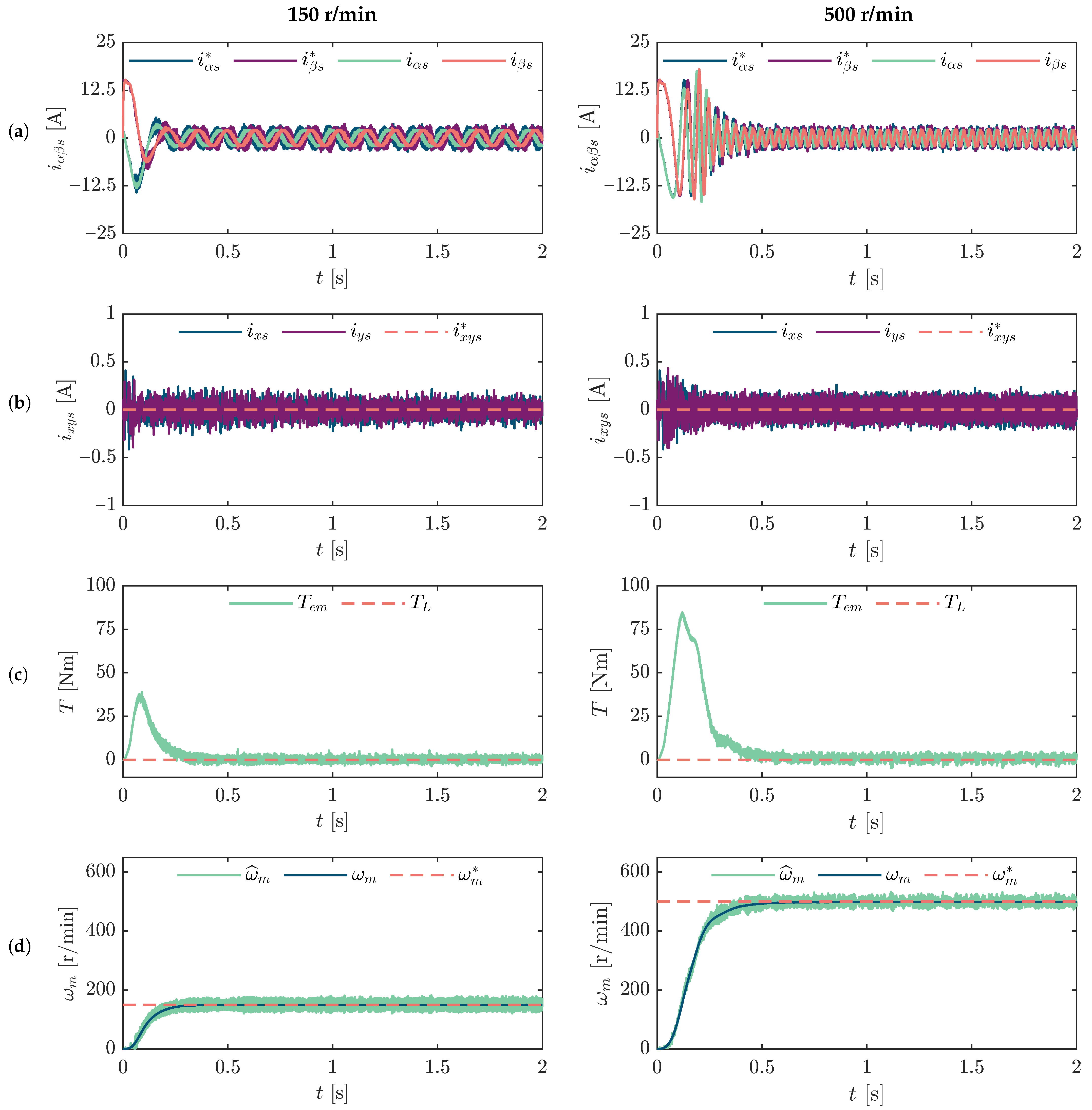
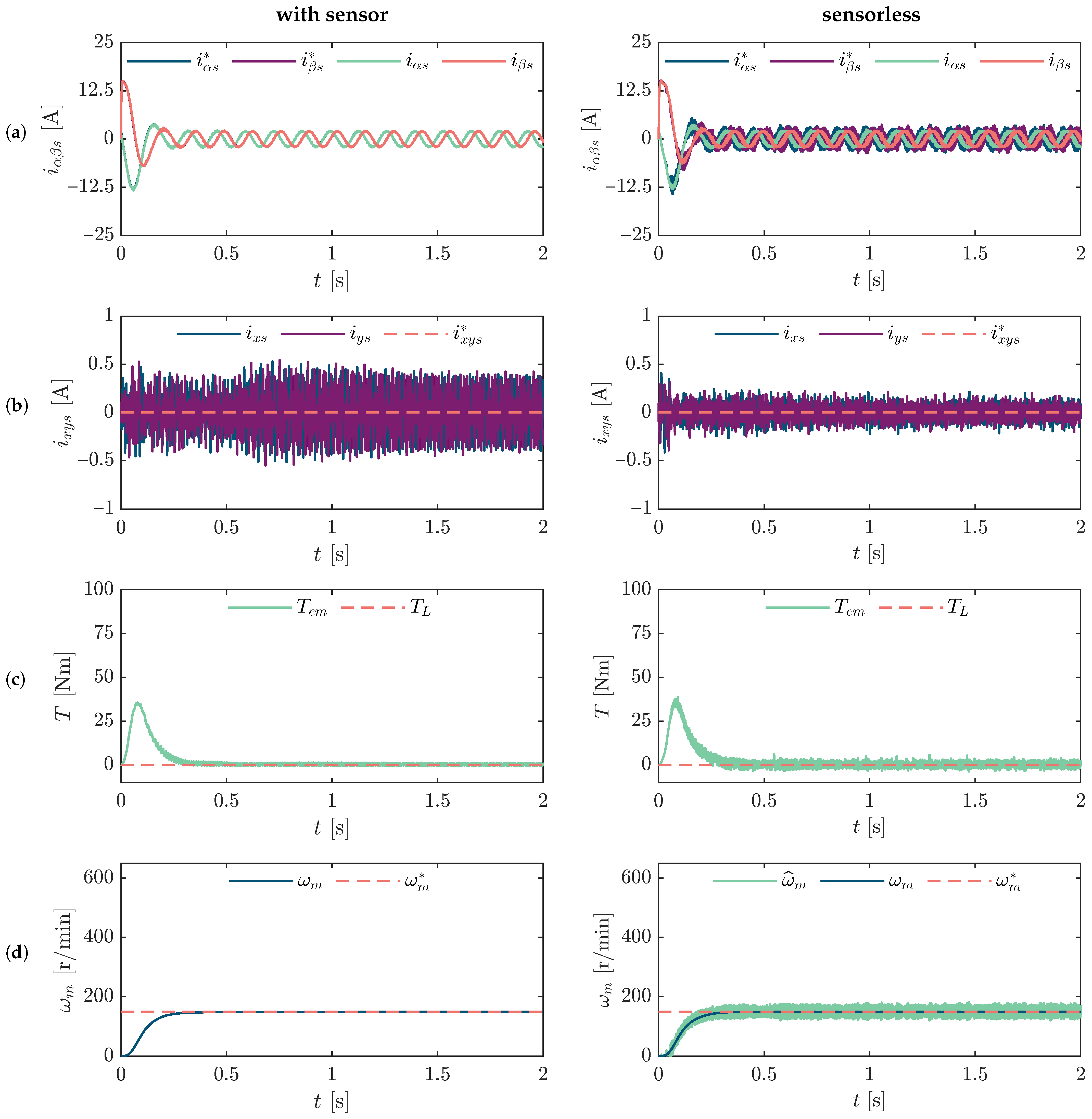
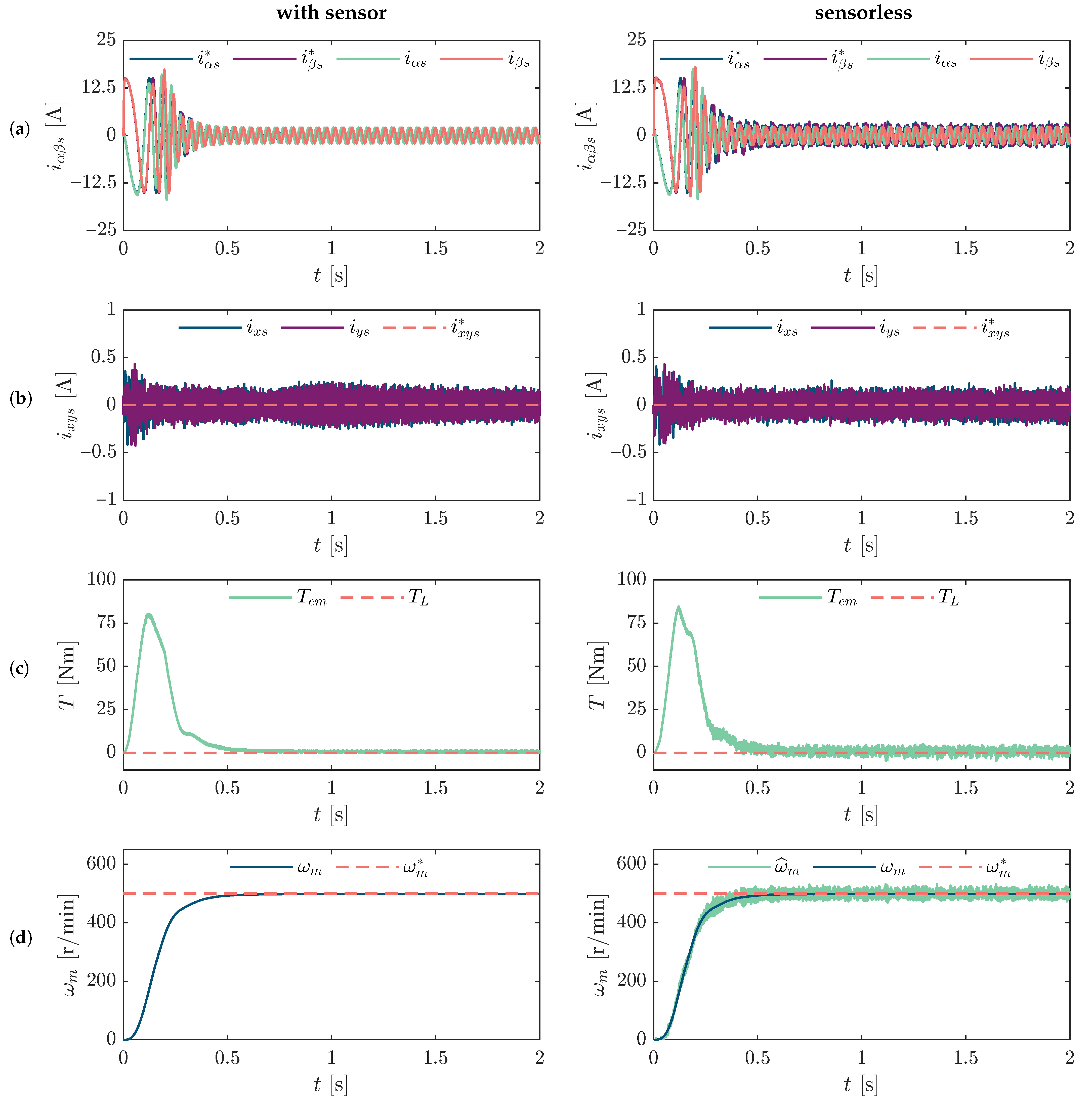
Figure 4a,b show the evolution of $\alpha \beta xy$ currents from transient to steady-state operation under two different speed conditions: 150 r/min and 500 r/min, using the sensorless approach. The response shows smooth dynamic behaviour and stable current waveforms, indicating proper control action during speed variations. Furthermore, Figure 4c,d depict the corresponding electromagnetic torque and speed response, respectively. The results confirm accurate tracking of the reference speed in both cases, with minimal steady-state error and acceptable torque ripple.

To further assess the performance of the proposed sensorless control strategy, a comparative study is conducted between two control configurations: one that utilizes a speed sensor (encoder-based) and the other that operates without a sensor, instead relying on the SMO approach. Figure 5 presents the comparison in low-speed operation, specifically at 150 r/min, which corresponds to approximately 7.5 Hz in terms of the electrical frequency of the stator. This scenario is particularly relevant, as sensorless techniques typically face greater challenges in maintaining robustness and accuracy at low speeds due to reduced observability and a lower signal-to-noise ratio.

As shown in Figure 5, the proposed method demonstrates excellent performance under these demanding conditions. The currents maintain consistent profiles, and the speed response closely follows the reference trajectory. Additionally, a reduction of the current components of the x-y subspace is observed in Figure 5b, which indicates improved current quality and reduced influence of parasitic harmonics, ultimately contributing to better efficiency and lower thermal stress on the drive.

In Figure 6, the same set of comparisons is repeated for a speed of 500 r/min. This operating point corresponds to a moderate-load condition, allowing the evaluation of the control strategy under higher stator frequencies, where sensorless techniques typically perform more reliably. The results again confirm that the proposed SMO-based approach is capable of maintaining accurate control of current and torque, as well as precise speed tracking, comparable to that of the encoder-based method.

4.2. Experimental Results

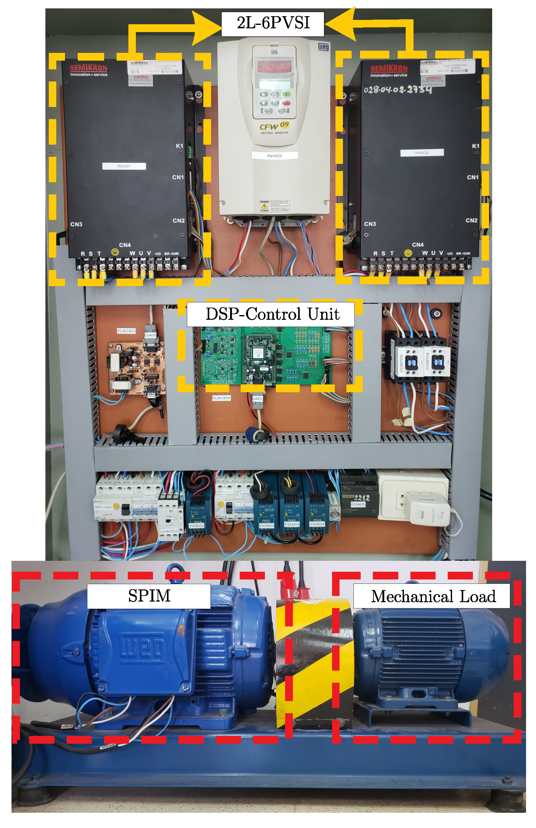
The experimental test bench setup is shown in Figure 7 and consists of a six-phase asymmetrical induction motor with an isolated neutral configuration, whose electrical and mechanical parameters are presented in Table 1.

A six-phase VSI drives the motor constructed using two three-phase SEMIKRON SKS 35F modules. Each module includes two Hall-effect sensors (LEM LA-55) that measure two of the three stator currents in each three-phase system, while the remaining stator currents are determined mathematically. A 325 V DC power supply is used for the DC-link. Both the control strategy and the SMO are implemented in discrete time using Euler’s method for numerical integration. The entire system is deployed on the MSK28335 development platform, which is based on the TMS320LF28335 floating-point DSP. The sampling frequency is set to 10 kHz, following the same configuration as in the simulation. A fixed d-current, $i_{ds}^{*}=2.5$ A, was considered and the observer gain $K_s=2000$.

The mechanical speed is measured using an optical sensor that generates a pulse train as the shaft rotates. Standard optical sensors can output several thousand pulses per revolution (ppr). In the experiments, a DFS60B-S1PB10000 encoder is used, providing 10,000 ppr. Moreover, digital signal processors typically include built-in functions for processing encoder pulses, such as the eQEP module in the TMS320F28335.

Finally, measurement data processing and graphical representation of the research outcomes were performed within the MATLAB computational environment.

4.2.1. Figures of Merit

The SMO performance is tested by calculating the Root Mean Squared Error (RMSE) between the reference values and the measured currents in every subspace monitored by the Hall sensors. The RMSE is calculated as:

$$\mathrm{RMSE}\left(i_{\vartheta s}\right)=\sqrt{{\displaystyle \frac{1}{\rho }}\sum _{k=k_0}^{k=k_0+\rho }{\left(i_{\vartheta s}\left(k\right)-i_{\vartheta s}^{*}\left(k\right)\right)}^2},$$

(51)

where $i_{\vartheta s}^{*}$ and $i_{\vartheta s}$ are the stator current references and the actual measurements with $\vartheta \in$ $\left\{\alpha ,\beta ,x,y\right\}$, $\rho$ is the total number of samples taken in an interval, and $k_0$ is the number taken as a starting point in steady-state. Integer numbers represent both.

Additionally, to assess the steady-state error, the Mean Value Error (MVE) of the speed estimation is defined as:

$$\mathrm{MVE}\left({\hat{\omega }}_m\right)={\displaystyle \frac{1}{\rho }}\sum _{k=k_0}^{k=k_0+\rho }\left|{\displaystyle \frac{{\omega }_m^{*}\left(k\right)-{\hat{\omega }}_m\left(k\right)}{{\omega }_m^{*}}}\right|\times 100\%.$$

(52)

4.2.2. Steady State and Transient Results

In Figure 8, the experimental results under an operating condition of 150 r/min are presented, including both the transient and steady-state responses. The left column shows the behaviour of the currents and mechanical speed when using the encoder, while the right column presents the results with the sensorless control based on the SMO.

Additionally, Figure 9a,b show the steady-state behaviour of the currents and mechanical speed under sensorless control at an operating speed of 150 r/min with an external load torque of approximately $40\mathrm{N}\mathrm{m}$ applied to the motor shaft.

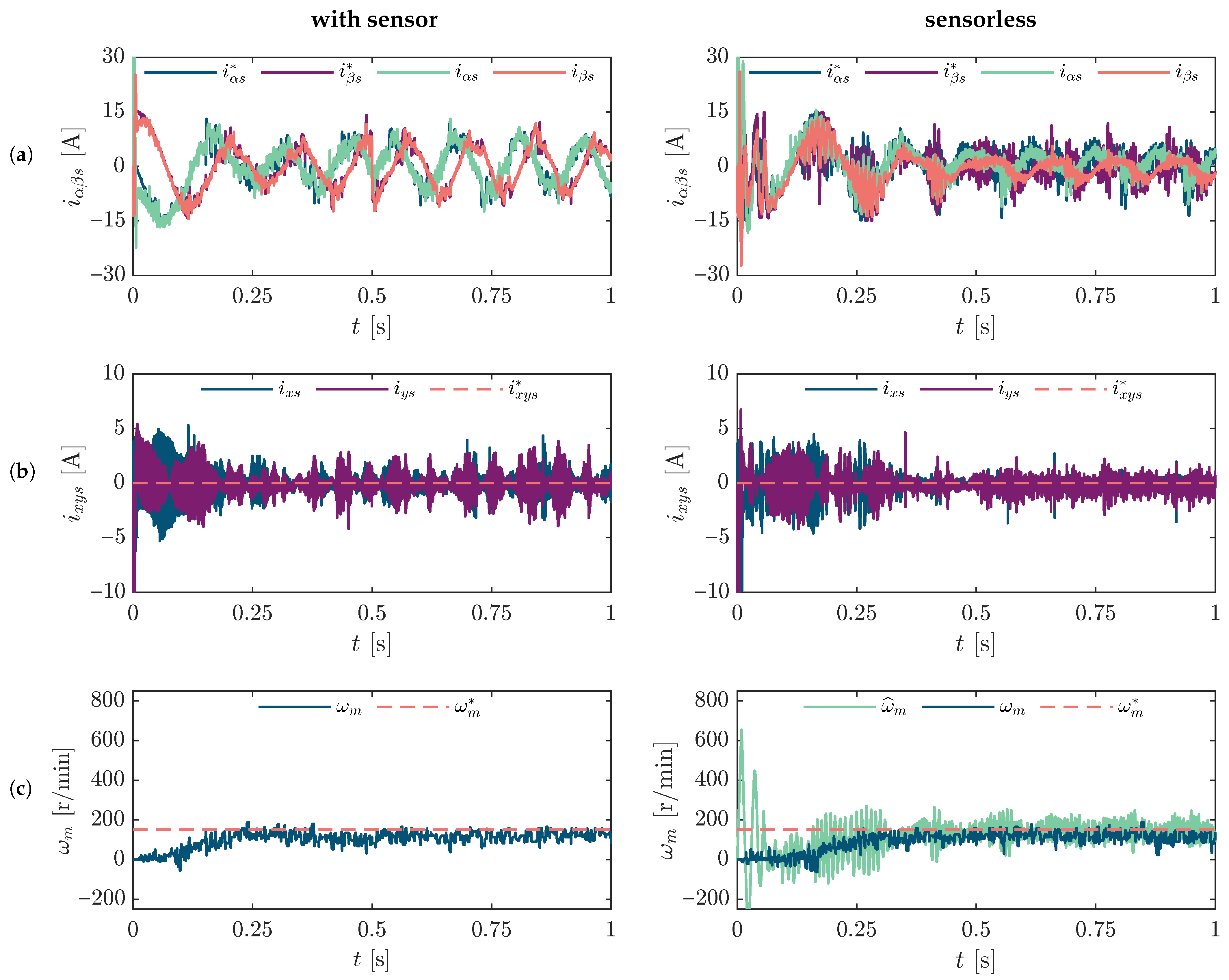
On the other hand, Figure 10 presents the behaviour of the $\alpha \beta xys$ currents and the speed tracking performance during a speed reversal from 150 r/min to –150 r/min, carried out using the proposed control technique. The results correspond to the operating conditions before and after the reversal. This type of test is particularly relevant in induction motor applications, as it enables the evaluation of the dynamic response to sudden changes in operating conditions. Successfully managing such transitions is essential in applications that require frequent direction changes or precise motion control, such as electric vehicles or industrial automation systems.

In Figure 11, the proposed SMO was tested under low-speed operating conditions, specifically at 20 r/min. The observer maintained stable and accurate estimation under these near-zero speed conditions. An increase in ripple was observed in the estimated speed due to the discontinuous nature of the sliding-mode algorithm. As expected at low speeds, the stator currents are also relatively small, which can reduce the signal-to-noise ratio and affect estimation quality. Nevertheless, the observer remained robust, and proper filtering ensured reliable performance without compromising control accuracy.

5. Discussion

Under low-speed operation, a comparison between the encoder-based control and the proposed sensorless technique presented in

Table 2. Performance of stator $\alpha \beta xy$ currents RMSE [A], THD [%], and rotor speed MVE [%] for FOC with mechanical sensor and FOC with SMO at 150 r/min reference speed under no-load conditions.

Test Condition: No-Load Operation
Figure of Merit	FOC with Sensor	FOC-SMO (Sensorless)
RMSE($i_{\alpha s}$)	2.8530	3.7168
RMSE($i_{\beta s}$)	2.1786	3.4020
THD($i_{\alpha s}$)	33.31	42.31
THD($i_{\beta s}$)	26.58	38.93
RMSE($i_{xs}$)	2.6280	1.1045
RMSE($i_{ys}$)	3.2826	1.9396
MVE(${\omega }_m$)	7.0122	2.5927

and

Table 3. Performance of stator $\alpha \beta xy$ currents RMSE [A], THD [%], and rotor speed MVE [%] for FOC with mechanical sensor and FOC with SMO at 150 r/min reference speed under load conditions.

Test Condition: Load Operation
Figure of Merit	FOC with Sensor	FOC-SMO (Sensorless)
RMSE($i_{\alpha s}$)	2.9426	3.7773
RMSE($i_{\beta s}$)	2.7161	3.1626
THD($i_{\alpha s}$)	27.20	58.30
THD($i_{\beta s}$)	27.81	52.01
RMSE($i_{xs}$)	3.2435	1.3391
RMSE($i_{ys}$)	3.7158	1.1720
MVE(${\omega }_m$)	7.4026	0.5785

reveals that the latter achieves a reduction of approximately 40% in the x-y subspace current components. This improvement contributes to lower parasitic losses and enhanced drive efficiency, particularly at low speeds. However, an increase of approximately 28% is observed in the tracking error of the currents in the $\alpha$–$\beta$ subspace with the sensorless approach. As for the THD in the $\alpha$–$\beta$ subspace, the FOC-SMO has a notorious increase compared to FOC with sensor. It must also be considered that the speed MVE is almost completely reduced with the FOC-SMO technique, so the amplitude of the currents is reduced, and considering that it has a lower signal-to-noise ratio, the THD is greater. However, with the FOC with sensor, the speed error is not completely corrected since a suboptimal speed control is used. This degradation can be attributed to the reduced back-EMF magnitude at low speeds, which compromises the observability of rotor dynamics. In the case of an SMO, this leads to reduced estimation accuracy due to weakened sliding conditions and increased sensitivity to noise. As a result, the current control in the $\alpha$–$\beta$ frame becomes less precise under low-speed operation.

The results in

Table 4. Performance of stator $\alpha \beta xy$ currents RMSE [A], THD [%], and rotor speed MVE [%] for FOC with SMO at reference speeds 150 and 300 r/min.

Figure of Merit	FOC-SMO 150 [r/min]	FOC-SMO 300 [r/mim]
RMSE($i_{\alpha s}$)	3.7168	4.5774
RMSE($i_{\beta s}$)	3.4020	3.9982
THD($i_{\alpha s}$)	42.31	66.87
THD($i_{\beta s}$)	38.93	63.21
RMSE($i_{xs}$)	1.1045	3.7386
RMSE($i_{ys}$)	1.9396	2.0642
MVE(${\hat{\omega }}_m$)	2.5927	0.2535

show that increasing the reference speed from 150 to 300 r/min leads to a significant improvement in rotor speed estimation accuracy, with the MVE dropping from 2.59 to 0.25%. This confirms the enhanced observability of the system at higher speeds, which benefits the performance of the SMO. However, this improvement is accompanied by an increase in current tracking error in both the $\alpha$–$\beta$ and x–y subspaces. For instance, RMSE($i_{xs}$) increases from 1.10 A to 3.74 A. This suggests a possible trade-off between estimation accuracy and current control performance under higher-speed operation, potentially due to suboptimal tuning of the current controllers at higher speeds. At the same time, optimal SMO gain design must be considered to ensure stability and acceptable chattering generation for the desired machine performance. It should also be noted that the six-phase machine must have optimal current control settings in both the ($\alpha$-$\beta$) and (x-y) subspaces.

6. Conclusions

This work has introduced the implementation of an SMO for sensorless speed control of an asymmetrical six-phase induction machine. The proposed method was first validated through simulation and later confirmed experimentally, demonstrating a high degree of consistency between the two sets of results.

The comparative analysis under no-load and load conditions at low speed demonstrates that the SMO-based control significantly outperforms the conventional FOC with mechanical sensors in rotor speed estimation accuracy, achieving much lower mean value errors (MVEs). While the SMO approach exhibits higher current tracking errors in the $\alpha$-$\beta$ subspace, it shows improved performance in the x-y current components, particularly under load. Moreover, the reduction in x-y subspace currents contributes to lower parasitic losses and enhanced drive efficiency in low-speed operation.

However, the sensorless strategy results in a notable increase in the THD of the $\alpha$-$\beta$ currents. This can be attributed to the reduced signal-to-noise ratio caused by the reduced current amplitude, which is a consequence of the improved speed regulation. Additionally, the limited back-EMF magnitude at low speeds compromises the observability of rotor dynamics, reducing the effectiveness of the SMO and introducing estimation inaccuracies due to weakened sliding conditions.

Further experimental evaluation revealed that the SMO-based sensorless control delivers more accurate rotor speed estimation at higher operating speeds, driven by enhanced system observability. Nonetheless, this improvement is accompanied by increased current tracking errors, emphasizing the trade-off between estimation precision and current control performance. This effect is likely associated with fixed current controller tuning, which may not be optimal across all operating conditions. To address this limitation, future work could investigate the integration of more advanced current control strategies to ensure consistent current regulation without compromising estimation accuracy.

References

1. Levi, E. Advances in Converter Control and Innovative Exploitation of Additional Degrees of Freedom for Multiphase Machines. IEEE Trans. Ind. Electron. 2016, 63, 433–448. [Google Scholar] [CrossRef]
2. Ayala, M.; Doval-Gandoy, J.; Rodas, J.; Gonzalez, O.; Gregor, R.; Delorme, L.; Romero, C.; Fleitas, A. Field-Weakening Strategy with Modulated Predictive Current Control Applied to Six-Phase Induction Machines. Machines 2024, 12, 178. [Google Scholar] [CrossRef]
3. Mohan, H.; Pathak, M.K.; Dwivedi, S.K. Sensorless control of electric drives—A technological review. IETE Tech. Rev. 2020, 37, 504–528. [Google Scholar] [CrossRef]
4. Holtz, J. Sensorless control of induction motor drives. Proc. IEEE 2002, 90, 1359–1394. [Google Scholar] [CrossRef]
5. Xu, D.; Wang, B.; Zhang, G.; Wang, G.; Yu, Y. A review of sensorless control methods for AC motor drives. CES Trans. Electr. Mach. Syst. 2018, 2, 104–115. [Google Scholar] [CrossRef]
6. Utrata, G.; Rolek, J. The Induction Motor MRAS-Based Speed Estimator Capable of Modelling the Slip Frequency Dependent Variability of the Rotor Impedance. Energies 2023, 16, 2591. [Google Scholar] [CrossRef]
7. Ayala, M.; Gonzalez, O.; Rodas, J.; Gregor, R.; Doval-Gandoy, J. A speed-sensorless predictive current control of multiphase induction machines using a Kalman filter for rotor current estimator. In Proceedings of the 2016 International Conference on Electrical Systems for Aircraft, Railway, Ship Propulsion and Road Vehicles &amp International Transportation Electrification Conference (ESARS-ITEC), Toulouse, France, 2–4 November 2016; IEEE: Piscataway, NJ, USA, 2016; pp. 1–6. [Google Scholar] [CrossRef]
8. Baiomy, N.; Abdelhafiz, M.M.; Mahgoub, A. Implicit Euler Discretization for Enhanced Sliding Mode Observer in Sensorless permanent magnet synchronous motor Control. IEEE Access 2024, 13, 4304–4314. [Google Scholar] [CrossRef]
9. Semenov, D.; Tian, B.; An, Q.T.; Sun, L. Position estimation for sensorless FOC of five-phase PMSM in electric vehicles. In Proceedings of the 2016 Australasian Universities Power Engineering Conference (AUPEC), Brisbane, Australia, 25–28 September 2016; pp. 1–5. [Google Scholar] [CrossRef]
10. Chen, L.; Jin, Z.; Shao, K.; Wang, H.; Wang, G.; Iu, H.H.C.; Fernando, T. Sensorless Fixed-Time Sliding Mode Control of PMSM Based on Barrier Function Adaptive Super-Twisting Observer. IEEE Trans. Power Electron. 2024, 39, 3037–3051. [Google Scholar] [CrossRef]
11. Xepapas, S.; Kaletsanos, A.; Xepapas, F.; Manias, S. Sliding-mode observer for speed-sensorless induction motor drives. IEE Proc.-Control Theory Appl. 2003, 150, 611–617. [Google Scholar] [CrossRef]
12. Holakooie, M.H.; Iwanski, G. An Adaptive Identification of Rotor Time Constant for Speed-Sensorless Induction Motor Drives: A Case Study for Six-Phase Induction Machine. IEEE J. Emerg. Sel. Top. Power Electron. 2021, 9, 5452–5466. [Google Scholar] [CrossRef]
13. Taheri, A.; Ren, H.; Holakooie, M.H. Sensorless Loss Model Control of the Six-Phase Induction Motor in All Speed Range by Extended Kalman Filter. IEEE Access 2020, 8, 118741–118752. [Google Scholar] [CrossRef]
14. Geng, Y.; Lai, Z.; Li, Y.; Wang, D.; Chen, R.; Zheng, P. Sensorless Fault-Tolerant Control Strategy of Six-Phase Induction Machine Based on Harmonic Suppression and Sliding Mode Observer. IEEE Access 2019, 7, 110086–110098. [Google Scholar] [CrossRef]
15. Rodas, J.; Gonzalez-Prieto, I.; Kali, Y.; Saad, M.; Doval-Gandoy, J. Recent Advances in Model Predictive and Sliding Mode Current Control Techniques of Multiphase Induction Machines. Front. Energy Res. 2021, 9, 729034. [Google Scholar] [CrossRef]
16. Zhao, Y.; Lipo, T. Space vector PWM control of dual three-phase induction machine using vector space decomposition. IEEE Trans. Ind. Appl. 1995, 31, 1100–1109. [Google Scholar] [CrossRef]
17. Duran, M.J.; Levi, E.; Barrero, F. Multiphase Electric Drives: Introduction. In Wiley Encyclopedia of Electrical and Electronics Engineering; John Wiley & Sons, Ltd.: New York, NY, USA, 2017; pp. 1–26. [Google Scholar] [CrossRef]
18. Barrero, F.; Prieto, J.; Levi, E.; Gregor, R.; Toral, S.; Duran, M.J.; Jones, M. An Enhanced Predictive Current Control Method for Asymmetrical Six-Phase Motor Drives. IEEE Trans. Ind. Electron. 2011, 58, 3242–3252. [Google Scholar] [CrossRef]
19. Le-Huy, H. Comparison of field-oriented control and direct torque control for induction motor drives. In Proceedings of the Conference Record of the 1999 IEEE industry Applications Conference. Thirty-forth IAS Annual Meeting (Cat. No. 99CH36370), Phoenix, AZ, USA, 3–7 October 1999; IEEE: Piscataway, NJ, USA, 1999; Volume 2, pp. 1245–1252. [Google Scholar] [CrossRef]
20. Khamis, A.A.H.; Abbas, A.M.A.; ALgoul, M.A.M. Comparative Study Between a Novel Direct Torque Control and Indirect Field Oriented Control of Three-Phase Induction Motors. In Proceedings of the 2022 IEEE 2nd International Maghreb Meeting of the Conference on Sciences and Techniques of Automatic Control and Computer Engineering (MI-STA), Sabratha, Libya, 23–25 May 2022; pp. 75–80. [Google Scholar] [CrossRef]
21. Harnefors, L.; Saarakkala, S.E.; Hinkkanen, M. Speed Control of Electrical Drives Using Classical Control Methods. IEEE Trans. Ind. Appl. 2013, 49, 889–898. [Google Scholar] [CrossRef]
22. Iqbal, A.; Moinuddin, S. Comprehensive Relationship Between Carrier-Based PWM and Space Vector PWM in a Five-Phase VSI. IEEE Trans. Power Electron. 2009, 24, 2379–2390. [Google Scholar] [CrossRef]
23. Utkin, V.; Guldner, J.; Shijun, M. Sliding Mode Control in Electro-Mechanical Systems; CRC Press: Boca Raton, FL, USA, 1999; Volume 34. [Google Scholar] [CrossRef]
24. Mossa, M.A.; Echeikh, H.; Iqbal, A.; Duc Do, T.; Al-Sumaiti, A.S. A Novel Sensorless Control for Multiphase Induction Motor Drives Based on Singularly Perturbed Sliding Mode Observer-Experimental Validation. Appl. Sci. 2020, 10, 2776. [Google Scholar] [CrossRef]
Figure 1. Typical configuration of an asymmetrical six-phase induction machine.
Machines 13 00639 g001
Figure 2. IRFOC scheme for an asymmetrical six-phase induction machine with isolated neutrals.
Machines 13 00639 g002
Figure 3. Block diagram of the proposed observer based on SMO.
Machines 13 00639 g003
Figure 4. Simulation results at different speeds with closed-loop speed estimation. (a) Stator current i α β s , (b) stator current i x y s , (c) electromagnetic torque, (d) mechanical speed.
Machines 13 00639 g004
Figure 5. Simulation results at 150 [r/min] with mechanical sensor and sensorless in closed loop. (a) Stator current i α β s , (b) stator current i x y s , (c) electromagnetic torque response without load, (d) mechanical speed.
Machines 13 00639 g005
Figure 6. Simulation results at 500 [r/min] with mechanical sensor and sensorless in closed loop. (a) Stator current i α β s , (b) stator current i x y s , (c) electromagnetic torque response without load, (d) mechanical speed.
Machines 13 00639 g006
Figure 7. Schematic of the experimental test bench.
Machines 13 00639 g007
Figure 8. Experimental results at 150 [r/min] with mechanical sensor and sensorless in closed loop. (a) Stator current i α β s , (b) stator current i x y s , (c) mechanical speed.
Machines 13 00639 g008
Figure 9. Experimental results at 150 [r/min] under a load torque of approximately 40 Nm. (a) Stator current i α β x y s , (b) mechanical speed.
Machines 13 00639 g009
Figure 10. Experimental results at 150 to 150 [r/min] sensorless in closed loop. (a) Stator current i α β x y s , (b) mechanical speed.
Machines 13 00639 g010
Figure 11. Experimental results at 20 [r/min]. (a) Stator current i α β x y s , (b) mechanical speed.
Machines 13 00639 g011