Optimization of Multi-Objective Problems for Sailfish-Shaped Airfoils Based on the Multi-Island Genetic Algorithm

Abstract

This article uses the sailfish outline as an airfoil profile to create a dual vertical-axis water turbine model for capturing wave and tidal current energy. A parametric water turbine model is built with the shape function perturbation and characteristic parameter description methods. Optimized by the multi-island genetic algorithm on the Isight platform, a CNC sample of the optimized model is made. Its torque and pressure are measured in a wind tunnel and compared with CFD numerical analysis results. The results show small differences between the numerical and experimental results. Both indicate that the relevant performance parameters of the turbine improved after optimization. During constant flow velocity measurement, the optimized axial-flow turbine has a pressure increase of 55% and a torque increase of 40%, while for the centrifugal turbine, the pressure increases by 60% and the torque by 12.5%. During constant rotational speed measurement, the axial-flow turbine’s pressure increases by 16.7%, with an unobvious torque increase. The Q-criterion diagram shows more vortices after optimization. This proves the method can quickly and effectively optimize the dual vertical-axis water turbine.

1. Introduction

The wave-tide energy coupling system has become a new trend in marine energy development by sharing mooring, power transmission, and control systems to reduce costs. The mainstream technical routes include floating platform integration. For example, the TriFrame structure of the Dutch company Tidal Kite, where the upper floating body captures wave energy and the lower suspended turbine utilizes tidal current energy in synergistic energy conversion. The ATIR platform of Spain’s Magallanes achieves bidirectional conversion through an intelligent scheduling system: the hydraulic PTO (Power Take-Off) system. The AI coordination module of the UK’s SABELLA balances the fluctuations of wave and current energy. In 2023, there were more than 17 coupling projects under construction globally. The SES-2000 platform in Scotland achieved 12 consecutive months of trouble-free operation. At present, the conversion efficiency of wave energy units can reach 18–22%, the conversion efficiency of tidal current energy is 42–47%, and the coupling gain is +8–12%. The annual power generation of wave energy units is 280 MWh, and that of tidal current energy is 3.2 GWh, with a synergistic increase of 35% in coupling gain. Typical cases include Portugal’s HiWave-5 project, which has a 5 MW coupled unit that has reduced the Levelized Cost of Energy (LCOE) to €0.21/kWh, and China’s Zhoushan LHD system, which combines tidal current turbines with oscillating floats, achieving a peak power of 4.3 MW.

Chunyun Shen et al. [1], based on traditional vertical-axis hydrokinetic turbines, utilized numerical calculations and experimental methods to investigate the effects of blade helicity and airfoil curvature on the energy conversion efficiency of vertical-axis hydrokinetic turbines in low flow velocity conditions. The results indicate that increasing the blade helical angle and airfoil curvature can better optimize the flow conditions around the turbine, significantly improving the energy conversion efficiency of vertical-axis turbines. Ahmed Gharib Yosry et al. [2] studied vertical-axis micro tidal turbines in low-velocity scenarios. It has been found that the upstream velocity has the most obvious effect on the turbine performance, and that the peak power coefficient is linked to the intensification in the blockage ratio. Khanjanpour et al. [3] used experimental and numerical analysis of the Hunter turbine, a vertical-axis turbine utilized for tidal energy. They found that the power coefficient increased as the submerged depth from a water-free surface increased, and after a specific depth, the output power remained constant. It was also observed that the minimum depth from a water-free surface for maximum power coefficient was three times the diameter of the turbine drum (3D). Konstantinos V. Kostas et al. [4] adopted a method combining supervised machine learning (ML) and technical artificial neural networks (ANNs) to train and calculate problems in airfoil and hydrofoil design. The authors demonstrated that a user-friendly real-time design assistant can be easily implemented and deployed with the identified models, whereas significant time savings with adequate accuracy can be achieved when ML tools are employed in design optimization. Bingchen Du et al. [5] used multi-fidelity deep neural networks (MFDNN) that combine high-fidelity (HF) and low-fidelity (LF) data for aerodynamic prediction and design optimization. As the insufficiency in the prediction accuracy of the optimal shapes appears when employing the non-updated MFDNN models, an update strategy is developed by tightly integrating the MFDNN models with the particle swarm optimization algorithm. To further reduce the time costs for updating models, a dual-threshold update strategy is then introduced, which can halve the time to evaluate HF data. Caraccio et al. [6] developed neural network architectures, comprising fully connected and transposed convolution layers, accurately inferring transformed field maps for incompressible flow around a NACA0012 airfoil based on the Reynolds (Re) number and angle of attack. By applying transfer learning to cGAN models trained with 15 cases for the prediction of velocity fields around the NACA4412 airfoil, the average error is up to 70% lower than training without weight transfer. Erfan Ghamati et al. Khanjanpour et al. [7] conducted a series of computational fluid dynamics (CFD) simulations using the hybrid-level improved Taguchi technique to determine the optimal hydrodynamic performance of the VAT turbine. The interaction relationships among four parameters—twist angle, camber position, maximum camber, and the chord/radius ratio—were studied using the analysis of variance (ANOVA) method. The results show that the power coefficient (Cp) of the optimized VAT turbine is increased by 24%, and the twisted and cambered blades can effectively suppress dynamic stall, thereby normalizing the spray vortices on the blades. Changming Li et al. [8] proposed an interactive framework for hydrofoil design and optimization based on deep learning, in which generative adversarial networks are used for parameterizing hydrofoil designs. The results show that the optimized hydrofoil shape has a larger lift–drag ratio than ordinary hydrofoils. This framework is effective and stable, capable of facilitating the design of tidal energy turbine rotors and providing higher power coefficients for hydrofoils.

In the field of water turbine optimization, there are mainly two effective methods: the analytical design method and the optimization design method [9]. The analytical design method is a strategy widely adopted by current engineering designers. When using this method, designers obtain accurate result data through CFD (computational fluid dynamics) calculations or experimental verifications according to the specific performance requirements of the water turbine [10]. Then, relying on their long-term, rich practical experience and solid theoretical knowledge, they make detailed and targeted adjustments to the design scheme. Moreover, this rigorous process is repeated continuously until the design scheme can perfectly meet the expected performance goals. However, this method often relies heavily on manual experience and repeated trials, and the process is relatively cumbersome.

The optimization design method realizes automatic optimization with the help of advanced optimization algorithms. The genetic algorithm, neural network algorithm, ant colony algorithm, etc., are typical representatives of such methods. Compared with the traditional analytical design method, the optimization design method demonstrates significant efficiency advantages, primarily attributed to its systematic and data-driven framework. It can accurately search for better design schemes in a shorter time, greatly shortening the design cycle and improving the design efficiency.

Brahim Aboutaib showed that, compared with the traditional uniform crossover operation, the parallel island model design can utilize the independence of the noisy hill-climbing process. By averaging through the multi-parent majority-vote crossover operation, it can effectively extract the fitness signal from the noise [11]. Jose Quevedo proposed that as the number of iterations increases, the reinforcement RL-GA maintains a high level of diversity in the population pool, and the obtained solutions are superior to those obtained by other methods (with an improvement of up to 11%) [12]. However, the traditional genetic algorithms often become trapped in the local optima, and their use requires substantial computational resources. The adoption of a modified version, known as the multi-island genetic algorithm (MIGA), effectively mitigates these challenges inherent in traditional GAs [13,14]. Zhongwei Zhao concluded that the results derived by GA-ANNs are more optimized than those derived by GWO-ANNs. GWO-ANNs tend to be a locally optimal solution [15]. Ke Zhang optimizes the solution distribution ratio and high-pressure generator outlet solution concentration in the AGX variable-effect cycle and obtains the maximum COP. The optimized COP increased by 10.65% on average, and 45.49% on maximum, and the optimized efficiency increased by 13.68% on average, and 42.29% on maximum [16].

In conventional hydraulic turbine design, researchers rely on experience and formulas to adjust parameters such as angle of attack, chord length, and thickness to achieve the required performance. This approach is time-consuming and highly dependent on individual expertise. In the research in this paper, after careful consideration, it was decided to use the multi-island genetic algorithm to conduct automatic optimization of the water turbine’s performance. This paper hopes to leverage the efficient searchability of this advanced algorithm to more quickly and accurately tap into the performance potential of the water turbine, thereby more efficiently improving the overall performance of the water turbine and providing a more scientific and efficient solution for the optimization design of the water turbine. The double-vertical-axis water turbine studied in this paper is shown in Figure 1 below.

2. Parametric Design of the Blade Surface Based on the Sailfish Profile

In previous research, the current authors, based on blade element theory, delved deeply into the influence of four parameters on the hydrodynamic performance of the airfoil with a sailfish profile. Blade element theory ingeniously simplifies the flow of fluid around the water turbine into a non-interfering two-dimensional flow form. However, in reality, due to the effect of the Coriolis force, the fluid has a radial flow, and its direction points towards the span of the blade. Given this, this paper focuses on considering the three-dimensional flow effect and comprehensively studies the influence of various parameters on the hydrodynamic performance of the water turbine. The schematic diagram of the hydraulic turbine structure can be seen in Figure 2.

Figure 3 below shows the elementary stage of the airfoil and its velocity triangle. After the fluid passes through the water turbine, the parameters of the gas change along the radial direction and are different from each other. For the convenience of in-depth research, this paper selects a position with a radius of r, intercepts an annular cascade with an elementary radius of ∆r, and unfolds it into a plane, thus obtaining the special-shaped elementary stage, as shown in the figure. In the representation of relevant parameters, subscript 1 represents the airfoil inlet, and subscript 2 represents the airfoil outlet.

Among them, w represents the relative velocity, and its velocity direction is tangent to the airfoil at the entry and exit points. u is the transport velocity (also known as circumferential velocity or linear velocity) at the radius r, and its magnitude satisfies the relationship u = ωr. c is the resultant velocity of the relative velocity and the transport velocity; that is, the actual velocity of the airflow when entering and leaving the water turbine. To facilitate this research and accurately obtain the aerodynamic performance of the elementary stage, this paper projects the actual velocity in the tangential and radial directions. The projection in the tangential direction is denoted as cu, and the projection in the radial direction is denoted as cm. The inlet and outlet angles of the airfoil are represented by β.

The following aerodynamic parameters can be obtained from the velocity triangle:

$$\mathrm{Q}=c_{m}A={\displaystyle \frac{\pi }{4}}{c}_m(D^2-d^2)$$

(1)

$$\mathrm{P}\mathrm{a}=\mathrm{\rho }\left(u_2{c}_{2u}-u_1{c}_{1u}\right)$$

(2)

$$\mathrm{T}=\mathrm{Q}(r_2{c}_{2u}-r_1{c}_{1u})$$

(3)

$${\beta }_1={cot}^{-1}{\displaystyle \frac{u_1-c_{1u}}{c_m}}={\mathrm{s}\mathrm{i}\mathrm{n}}^{-1}{\displaystyle \frac{c_m}{{\omega }_1}}$$

(4)

$${\beta }_2={cot}^{-1}{\displaystyle \frac{u_2-c_{2u}}{c_m}}={\mathrm{s}\mathrm{i}\mathrm{n}}^{-1}{\displaystyle \frac{c_m}{{\omega }_2}}$$

(5)

The relationships among the inlet and outlet angles, the airfoil curvature K, and BVF (Boundary Vorticity Flux theory) are as follows:

$${\overline{\sigma }}_p={\displaystyle \frac{\dot{m}{\overline{V}}_x}{2\rho }}\left[{\displaystyle \frac{dK}{dx}}{sec}^2\beta +3K^2{sec}^3\beta tan\beta \right]$$

(6)

${\overline{\sigma }}_p$ represents BVF, $\dot{m}$ is the mass flow rate, and ${\overline{V}}_x$ is the circumferential average of the inlet axial velocity. If the performance of the water turbine is determined, neither $\dot{m}$ nor ${\overline{V}}_x$ will change. The change in the BVF performance of the elementary stage $\beta$ is only related to the inlet and outlet angles. Therefore, the performance improvement of the water turbine can be studied by optimizing the installation angle of the turbine blades and the airfoil curvature.

From the velocity triangle diagram, we can preliminarily infer that the following relatively quick methods can be used to increase the torque of the water turbine (i.e., increase the output shaft power and thus the power generation):

(1) Increase the flow rate of the water turbine

Increasing the flow rate of the water turbine means increasing $c_m$. There are several specific ways to achieve this: one is to increase the blade installation angle while keeping the chord length constant; the second is to lengthen the chord length of the airfoil when the installation angle is fixed; in addition, the installation angle and the chord length can be increased simultaneously. Through these methods, the flow rate of the water turbine can be effectively increased, creating conditions for increasing the torque.

(2) Increase the rotation speed of the water turbine

Increasing the rotation speed of the water turbine is also a feasible method. Generally speaking, it is relatively easy to achieve this goal by increasing the rotation speed. However, it should be noted that as the rotation speed continues to increase, the structural strength of the water turbine will face a huge challenge. Therefore, in the process of increasing the rotation speed, the structural design and material properties of the water turbine must be fully considered to ensure that it can withstand the corresponding load.

(3) Adjust the blade diameter

Increasing the blade diameter at the outlet while reducing the blade diameter at the inlet can also help increase the torque of the water turbine. However, the applicability of this method varies depending on the type of water turbine. For axial-flow water turbines, since the outlet and inlet diameters are the same, this method cannot be used for adjustment; for centrifugal water turbines, this method can be used to optimize the performance. In practical applications, the adjustment strategy needs to be reasonably selected according to the specific type and working requirements of the water turbine.

In the framework of airfoil design, parameters of the water turbine, such as the number of blades, installation angle, bow angle, hub ratio, thickness, and angle of attack, are of critical importance. The parametric modeling of the airfoil precisely adjusts these parameters to ingeniously realize the ever-changing blade shapes, then constructs a three-dimensional model of the impeller, and accurately predicts its performance. The parametric representation of the airfoil directly influences the quality of the optimization results. An excellent parametric model should have the following two characteristics: Firstly, controllability. The geometric profile function of the airfoil needs to be continuous and smooth, and the control parameters need to be independent of each other, enabling precise control of the local changes in the airfoil profile line to vividly present the required airfoil geometric shape. Secondly, completeness. In the vast design space, the parametric modeling of the airfoil should be able to describe the airfoil that meets the design requirements as comprehensively as possible with fewer control parameters [17,18].

The optimization design methods for airfoils can be broadly classified into direct methods and indirect methods, exhibiting distinct characteristics [19]. The direct method takes the aerodynamic performance of the airfoil as a clear goal and directly conducts optimization design on its shape. Common methods include the B-spline (NURBS) modeling method [20,21], the Bezier curve modeling method, the analytical function perturbation method, the Hicks–Henne shape function [22,23] perturbation method, the characteristic parameter description method, etc. The indirect method focuses on solving the classic aerodynamic problem; that is, accurately solving the aerodynamic shape that matches the given target pressure distribution. In this paper, the advantages of the shape function perturbation method and the characteristic parameter description method are ingeniously combined to carefully construct the parametric model of the airfoil.

When performing parametric modeling of the airfoil cross-section, it is mainly composed of three parts: the reference airfoil, the shape function, and the control parameters [24]. Among them, the sailfish profile is selected as the reference airfoil. On this basis, by flexibly adjusting the control parameters, the basic airfoil will change accordingly, thus accurately achieving the goal of adjusting the airfoil shape. The expression of the shape function is as follows:

$$\mathrm{x}\left({\epsilon }_1{\epsilon }_2\theta \alpha \right)=x_0\left({\epsilon }_1{\epsilon }_2\theta \alpha \right)+\sum _{i=1}^n{a}_i{f}_i\left({\epsilon }_1{\epsilon }_2\theta \alpha \right)$$

(7)

$$\mathrm{y}({\epsilon }_1{\epsilon }_2\theta \alpha )=y_0({\epsilon }_1{\epsilon }_2\theta \alpha )+\sum _{i=1}^n{b}_i{f}_i({\epsilon }_1{\epsilon }_2\theta \alpha )$$

(8)

$$\mathrm{z}({\epsilon }_1{\epsilon }_2\theta \alpha )=z_0({\epsilon }_1{\epsilon }_2\theta \alpha )+\sum _{i=1}^n{c}_i{f}_i({\epsilon }_1{\epsilon }_2\theta \alpha )$$

(9)

where:

x, y, z—Coordinates of the new airfoil;

$x_0$, $y_0$, $z_0$—Coordinates of the reference airfoil;

${\epsilon }_1$—Chord length coefficient;

${\epsilon }_2$—Thickness coefficient;

θ—Bow angle;

α—Installation angle;

n—Number of airfoil control points;

$a_i{,b}_i{,c}_i$—Control parameters;

$f_i\left({\epsilon }_1{\epsilon }_2\theta \alpha \right)$—Control function.

$$f_i\left({{\displaystyle \epsilon }}_1{{\displaystyle \epsilon }}_2\theta \alpha \right)=\left\{\begin{array}{c}(({{\displaystyle m}}_{xi}-{{\displaystyle m}}_{xn})*\cos \alpha -({{\displaystyle m}}_{yi}-{{\displaystyle m}}_{yn})*\sin \alpha +{{\displaystyle m}}_{xn}{{\displaystyle +h}}_{xi}/2)*{{\displaystyle \epsilon }}_1\\ ({{\displaystyle m}}_{xi}-{{\displaystyle m}}_{xn})*\sin \alpha +({{\displaystyle m}}_{yi}-{{\displaystyle m}}_{yn})*\cos \alpha +{{\displaystyle m}}_{yn}+{{\displaystyle h}}_{yi}/2+{{\displaystyle \sigma }}_M\\ {{\displaystyle \sigma }}_M=(1-\cos (0.5*\theta ))/2/\sin (0.5*\theta )\end{array}\right.$$

(10)

In the formula:

$m_{xi}$—The x-coordinate of the i-th point on the mean camber line;

$m_{yi}$—The y-coordinate of the i-th point on the mean camber line;

$h_{xi}$—The x-coordinate of the airfoil thickness at the i-th point;

$h_{yi}$—The y-coordinate of the airfoil thickness at the i-th point;

${\delta }_M$—The maximum airfoil camber height.

The description of the airfoil characteristic parameters is shown in Figure 4. The airfoil is divided into 60 control points, with 30 control points on the upper surface (suction surface) and 30 control points on the lower surface (pressure surface). L is the airfoil chord length, $\theta$ is the bow angle, $\alpha$ is the installation angle, and $\delta$ is the thickness at each design point. Meanwhile, the chord length coefficient ${\epsilon }_1$ and the thickness coefficient ${\mathrm{\epsilon }}_2$ are defined. To solve this problem, this paper uses the installation angle to approximately replace the angle of attack. The installation angle is the angle between the chord length and the circumferential direction, as shown in Figure 4 below. This replacement method has a certain degree of rationality and feasibility in model construction.

By precisely adjusting the parameters of each control characteristic of the airfoil, as well as the chord length and thickness coefficients, the coordinates of the control points of the airfoil cross-section can be accurately output. Subsequently, with the powerful macro-processing module of the CATIA 3D software, these coordinates can be automatically interpolated to generate a smooth spline curve. Based on this spline curve, a 3D model of the airfoil and even a complete water turbine model can be further constructed.

This process has significant advantages. On the one hand, it can effectively avoid the situation of an irregular blade shape, making the blade shape more smooth and natural; on the other hand, when drawing the grid later, it can ensure a smooth transition of the grid, greatly reducing the calculation singularities caused by problems in the 3D model construction. This not only improves the quality of the model but also lays a solid foundation for the subsequent numerical calculation and analysis work, which helps to obtain more accurate and reliable results. The coordinate values of the reference airfoil are shown in

Table 1. Coordinate data of the control points of the baseline airfoil.

X/L [%]	XNPS	YNPS	ZNPS	XPPS	YPPS	ZPPS	ATK	MCL
0	17.313	66.442	0	17.313	66.442	0	0	66.442
3.3	16.754	67.649	0	16.228	65.49	0	2.159	66.5695
6.6	15.311	67.49	0	15.09	64.555	0	2.935	66.0225
9.9	13.849	67.316	0	14.07	63.492	0	3.824	65.404
13.2	12.386	67.452	0	12.932	62.561	0	4.891	65.0065
16.5	10.996	67.936	0	11.746	61.686	0	6.25	64.811
19.8	9.654	68.545	0	10.499	60.902	0	7.643	64.7235
23.1	8.304	69.131	0	9.223	60.165	0	8.966	64.648
26.4	6.844	69.208	0	7.922	59.473	0	9.735	64.3405
29.7	5.394	68.952	0	6.587	58.849	0	10.103	63.9005
33	4.027	68.409	0	5.224	58.289	0	10.12	63.349
36.3	2.837	67.544	0	3.845	57.769	0	9.775	62.6565
39.6	1.63	66.7	0	2.46	57.264	0	9.436	61.982
42.9	0.343	65.983	0	1.076	56.76	0	9.223	61.3715
46.2	−0.948	65.273	0	−0.309	56.255	0	9.018	60.764
49.5	−2.236	64.556	0	−1.694	55.751	0	8.805	60.1535
52.8	−3.527	63.846	0	−3.079	55.247	0	8.599	59.5465
56.1	−4.819	63.136	0	−4.463	54.741	0	8.395	58.9385
59.4	−6.111	62.427	0	−5.897	54.421	0	8.006	58.424
62.7	−7.408	61.727	0	−7.37	54.36	0	7.367	58.0435
66	−8.707	61.031	0	−8.828	54.546	0	6.485	57.7885
69.3	−9.988	60.303	0	−10.299	54.498	0	5.805	57.4005
72.6	−11.244	59.532	0	−11.77	54.414	0	5.118	56.973
75.9	−12.513	58.782	0	−13.243	54.419	0	4.363	56.6005
79.2	−13.815	58.094	0	−14.711	54.314	0	3.78	56.204
82.5	−15.11	57.39	0	−16.147	53.984	0	3.406	55.687
85.8	−16.383	56.647	0	−17.526	53.472	0	3.175	55.0595
89.1	−17.685	55.959	0	−18.842	52.809	0	3.15	54.384
92.4	−19.036	55.37	0	−20.215	52.277	0	3.093	53.8235
95.7	−20.392	54.792	0	−21.469	52.558	0	2.234	53.675
100	−21.584	53.973	0	−21.584	53.973	0	0	53.973

.

The secondary development of CATIA mainly includes two methods: in-process access and out-of-process access [25,26].

In-process access means that the script runs in the same process as CATIA V5-6R2012, and the macro script commands are executed by CATIA’s script engine. This method closely integrates the script with the software, and the software’s engine efficiently processes the script instructions.

Out-of-process access is different. Its script is not directly called by CATIA. Instead, CATIA is regarded as an OLE (Object Linking and Embedding) automation server, and external programs access the internal objects of CATIA through the COM interface. Based on AUTOMATION, out-of-process access can perform operations such as creating or modifying sketches, decoding, customizing, and controlling CATIA outside a process. Moreover, when making each modification to the CATIA objects outside the process, it can be decided whether to keep the modification according to the situation, to maintain synchronization between the two processes [27].

In this paper, out-of-process access is carried out based on the open Isight platform. During the implementation process, CATIA is flexibly called and its update is controlled to meet specific development requirements.

Appendix A clearly shows the airfoil parametric modeling process. The specific operations are as follows: First, input the data in Table 1 into the PointSplineLoftFromExcel file in the CATIA installation directory. Then, select Feuil1.main in the “Tools”-“Macro”-“Macro” menu and click “Execute”. At this time, a dialog box will pop up. Users can input 1, 2, or 3 on the keyboard according to actual needs (where 1 represents all points, 2 represents spline curves, and 3 represents scanned surfaces) to complete the import of the basic airfoil. The imported data are shown in Figure 5.

Then, start the CATIA formula editing command to create the coordinates of the airfoil contour points. A total of six coordinate points need to be created. Based on the input basic airfoil, input Formulas (1)–(6) in sequence. To ensure the smoothness of the curve and reduce the singularity problems caused by the modeling, the spline curve function in the generative surface is used to generate the airfoil contour line. The generated curve is shown in Figure 5.

After this, open the CATIA design table and export the airfoil control parameters. The specific content is shown in

Table 2. (a) Control parameter points of the axial-flow turbine airfoil; (b) Control parameter points of the centrifugal turbine airfoil.

(a)
No.	Parameter	Value	Upper Bound	Lower Bound
1	hubradius (mm)	11.0	NA	NA
2	radius2 (mm)	20.75	NA	NA
3	radius3 (mm)	29.0	NA	NA
4	radius4 (mm)	37.25	NA	NA
5	ringradius (mm)	45.5	NA	NA
6	Proportional Coefficient of Airfoil Thickness_hub	1	0.8	1.5
7	Proportional Coefficient of Airfoil Thickness2	1	0.8	1.5
8	Proportional Coefficient of Airfoil Thickness3	1	0.8	1.5
9	Proportional Coefficient of Airfoil Thickness4	1	0.8	1.5
10	Proportional Coefficient of Airfoil Thickness5	1	0.8	1.5
11	Installation Angle_deg_section1 (deg)	50	45	55
12	Installation Angle_deg_section2 (deg)	45	40	50
13	Installation Angle_deg_section3 (deg)	40	35	45
14	Installation Angle_deg_section4 (deg)	35	30	40
15	Installation Angle_deg_section5 (deg)	30	25	35
16	Chord Length Ratio Coefficient_section1	1	0.8	1.1
17	Chord Length Ratio Coefficient_section2	1	0.9	1.2
18	Chord Length Ratio Coefficient_section3	1	1.0	1.3
19	Chord Length Ratio Coefficient_section4	1	1.0	1.5
20	Chord Length Ratio Coefficient_section5	1	1.0	1.5
21	Arcuate Angle(θc)_deg_section1 (deg)	15	15	25
22	Arcuate Angle(θc)_deg_section2 (deg)	15	15	25
23	Arcuate Angle(θc)_deg_section3 (deg)	15	15	25
24	Arcuate Angle(θc)_deg_section4 (deg)	15	15	25
25	Arcuate Angle(θc)_deg_section5 (deg)	15	15	25
26	Balde Number	5	NA	NA
(b)
No.	Item	Para.	Upper Bound	Lower Bound
1	‘ArcuateAngle(θc)_deg’ (deg)	17.46	15	25
2	InstallationAngle_deg (deg)	39.00	0	55
3	ChordLengthRatioCoefficient	0.98	0.8	1.5
4	ProportionalCoefficientOfAirfoilThickness	1.25	0.8	1.5
5	baldeNumber	5	NA	NA

. To enable CATIA to automatically update and generate a three-dimensional model according to the adjusted control parameters, this paper first writes a CATIA calling program. Subsequently, a script text is carefully written in Visual Basic (VB). With the help of this text, the data parameters in CATIA can be updated, thereby realizing the automatic generation and dynamic update of 3D data.

3. Multi-Island Genetic Algorithm

The genetic algorithm (GA), first proposed by Professor Holland [28], is an algorithm that simulates the natural evolution process in the biological world to search for optimal solutions. This algorithm cleverly draws on the principles of biological evolution in nature, providing new ideas for solving various complex problems.

The multi-island genetic algorithm (MIGA) is an optimization and improvement based on the genetic algorithm (GA). It not only inherits the advantages of the general genetic algorithm but also ingeniously divides multiple populations into several “islands”. In each “island” population, the general genetic algorithm performs regular operations, including migration, selection, crossover, and mutation, similar to processes occurring in independent systems. Moreover, individuals are periodically exchanged between these “islands”, analogous to organismal interactions across different regions. This unique design method enhances the algorithm’s vitality by promoting cross-population genetic diversity. It can not only effectively maintain the diversity of the population but also powerfully suppress the phenomenon of premature convergence, avoid the optimization process falling into the trap of locally optimal solutions, and thus have a more excellent global solving ability and computational efficiency [29]. Its specific process is shown in Figure 6, and the parameter values of the multi-island genetic algorithm are listed in

Table 3. Parameters of the multi-island genetic algorithm.

No.	Name	Parameter Definition	Para.
1	Sub-population size	Sub-Population Size	10
2	Number of islands	Number of Islands	2
3	Number of generations	Number of Generations	8
4	Rate of crossover	Rate of Crossover	1
5	Rate of mutation	Rate of Mutation	0.01
6	Rate of migration	Rate of Migration	0.01
7	Interval of migration	Interval of Migration	5
8	Elite size	Elite Size	1
9	Rel tournament size	Rel Tournament Size	0.5
10	Penalty base	Penalty Base	0
11	Penalty multiplier	Penalty Multiplier	1000
12	Penalty exponent	Penaltv Exponent	2
13	Default variable bound (Abs Val)	Default Variable Bound (Abs Val)	1000
14	Max failed runs	Max Failed Runs	5
15	Failed run penalty value	Failed Run Penalty Value	1030
16	Failed run objective value	Failed Run Objective Value	1030

.

Using the multi-island genetic algorithm for airfoil optimization is a rather common and effective method. This is because the genetic algorithm itself has the characteristic of global convergence and does not rely on gradient information. The algorithm exhibits high adaptability and can be applied to discontinuous, discrete, and non-convex optimization problems, featuring a broad application scope and excellent robustness [30]. It directly uses the objective function value as the search information and accurately measures the goodness of individuals through the fitness function value, without the need for the complex process of differentiating the objective function value. This simple and efficient way makes the genetic algorithm stand out among many optimization algorithms and shows a high degree of superiority [31].

The steps of airfoil optimization using the multi-island genetic algorithm are as follows:

• Define the initial population: Clearly define the airfoil coefficients such as the blade installation angle, thickness coefficient, chord length coefficient, camber angle, radius, and the number of blades, establishing an initial framework for the entire optimization process.
• Define the objective function: Take the impeller torque as the objective function to point out the direction for the algorithm.
• Define multiple islands: This paper is carefully designed to have two islands, and each island will become an independent evolutionary space.
• Define the genetic algorithm for each island: Within each island, operations including selection, crossover, and mutation are systematically performed, analogous to evolutionary processes occurring in independent ecological systems. The specific process is shown in Figure 6.
• Define the inter-island migration count: The number of migrations is rationally configured to enhance population diversity, analogous to introducing novel genetic material into biological populations to mitigate the algorithm’s risk of premature convergence.
• Define the next-generation population: According to the objective function, carefully select the next-generation population from the current population to promote the continuous progress of the evolutionary process.
• Repeat the genetic algorithm within the islands and the migration actions between the islands according to the new population, and continue the iteration until the requirements of the objective function are met.
• Obtain the optimal individual: After a series of evolutions and screenings, finally find the optimal individual that best meets the requirements, completing the mission of airfoil optimization.

• Sub-population size

  ▪

  The number of individuals in each sub-population (island).

  ▪

  In this case, each island contains 10 individuals, and multiple islands evolve in parallel to increase population diversity.

• Number of islands

  ▪

  The number of sub-populations running in parallel in the multi-island genetic algorithm.

  ▪

  Two islands are used in this study, with individuals exchanged through migration operations.

• Number of generations

  ▪

  The maximum number of evolutionary generations before the algorithm terminates.

  ▪

  Set to eight generations in this case, and optimization stops once this number is reached.

• Rate of crossover

  ▪

  The proportion of individuals participating in crossover operations per generation.

  ▪

  A value of 1 indicates that 100% of individuals undergo crossover to generate new solutions.

• Rate of mutation

  ▪

  The probability of mutation for each gene.

  ▪

  The value (1%) means there is a 1% chance of randomly altering gene values, preventing the algorithm from falling into local optima.

• Rate of migration

  ▪

  The proportion of individuals transferred from one island to another during each migration operation.

  ▪

  The value (1%) indicates that 1% of individuals have migrated to promote genetic exchange between islands.

• Interval of migration

  ▪

  The generational gap between two consecutive migration operations.

  ▪

  Migrations are performed every five generations to balance exploration and exploitation capabilities.

• Elite size

  ▪

  The number of optimal individuals directly retained for the next generation in each generation.

  ▪

  Set to 1 to ensure the best solution is not destroyed by crossover or mutation.

• Rel tournament size

  ▪

  The proportion of individuals randomly selected for tournament selection.

  ▪

  A value of 0.5 means 50% of individuals are competed in each selection; smaller values increase selection pressure.

• Penalty base

  ▪

  The base value of the penalty function for constraint violations.

  ▪

  Set to 0, meaning no base penalty is applied—penalties are only imposed on solutions violating constraints.

• Penalty multiplier

  ▪

  The amplification factor for the degree of constraint violation.

  ▪

  A value of 1000 significantly increases the objective function value for constraint-violating solutions.

• Penalty exponent

  ▪

  The exponential term in the penalty function.

  ▪

  Set to 2, meaning the penalty is proportional to the square of the constraint violation degree.

• Default variable bound (Abs Val)

  ▪

  The absolute upper limit of the variable value range.

  ▪

  A value of 1000 indicates that the default range for the variables is [−1000, 1000], preventing an excessively large solution space.

• Max failed runs

  ▪

  The threshold for terminating the algorithm when no better solutions are found consecutively.

  ▪

  A value of 5 means the algorithm terminates early if no improvement occurs for five consecutive generations.

• Failed run penalty value

  ▪

  The penalty value for invalid solutions. A value of 1030 represents an extremely high penalty, making it almost impossible for invalid solutions to be selected.

• Failed run objective value

  ▪

  The substitute objective function value for invalid solutions.

  ▪

  Similar to the penalty value, it is used to mark infeasible solutions.

4. Determination of Parameters for Multi-Objective Problems

The core objective of a dual-vertical-axis water turbine power generation system is to capture as much mechanical energy as possible under the same hydrological conditions and then convert it into more electrical energy. To facilitate computational analysis, the following assumptions are made in this paper: first, the tidal current flows at a constant speed; second, the waves fluctuate up and down at a constant speed; and third, the power generation device remains stationary in the water area. The basic concept of a multi-objective problem is to find a set of optimal solution sets that satisfy all the constraints and requirements of each objective function. In practical applications, for a dual-vertical-axis water turbine power generation system, how to maximize the energy capture coefficient under the same flow velocity and wave conditions has become a crucial problem that needs to be solved urgently. The relevant objective functions and constraints are as follows [32]:

$$\mathrm{M}\mathrm{a}\mathrm{x}\mathrm{F}\left(\mathrm{x}\right)=[\epsilon 1,\epsilon 2,\theta ,\alpha ]$$

(11)

$$\mathrm{s}.\mathrm{t}.\left\{\begin{array}{c}{\mathrm{g}}_{\mathrm{i}}\left(x\right)\le 0,i=\mathrm{1,2},\cdots ,k\\ {\mathrm{h}}_{\mathrm{i}}\left(x\right)\le 0,i=\mathrm{1,2},\cdots ,p\\ {\mathrm{a}}_{\mathrm{i}}\le {\mathrm{x}}_{\mathrm{i}}\le {\mathrm{b}}_{\mathrm{i}},i=\mathrm{1,2},\cdots ,n\end{array}\right.$$

(12)

In the formula, n is the number of design variables; k and p are the numbers of constraints; and ${\mathrm{a}}_{\mathrm{i}}$ and ${\mathrm{b}}_{\mathrm{i}}$ are the upper and lower limits of the i-th design variable.

The upper and lower limits of the design variables are shown in Table 2, where $\epsilon 1,\epsilon 2,\theta ,\alpha$ correspond to Arcuate Angle(θc), Installation Angle, Chord Length Ratio Coefficient, and Proportional Coefficient of Airfoil Thickness, respectively. The upper limits of the objective functions are shown in

Table 4. Parameters of the objective function.

No.	Para.	Upper Bound	Lower Bound
1	Axial-flow turbine torque [Nmm]	100	10
2	Axial-flow turbine head [Pa]	50	10
3	Centrifugal turbine torque [Nmm]	1000	300
4	Centrifugal turbine head [Pa]	50	10

, where $g_i\left(x\right)$ and $h_i\left(x\right)$ correspond to turbine torque and turbine head, respectively.

5. Optimization of Water Turbines Based on Isight

In the research in this paper, the powerful functions of the Isight tool are fully utilized to integrate software such as CATIA, ICEM, CFX_Pre, CFX_Solver, and CFX_POST.

This integration enables automatic updates and synchronization across the water turbine’s three-dimensional modeling, mesh generation, pre-processing software, calculation software, and post-processing software. The interconnected workflow ensures close collaboration and synergy among all stages, enhancing overall efficiency. At the same time, the multi-island genetic algorithm is used in this paper for optimization in the hope of finding the optimal solution. The details of the parameter settings of the multi-island genetic algorithm are shown in Table 3. Specifically, a sub-population size of 10, an island number of 2, and an evolutionary iterations number of 8 generations are defined in this paper. After the calculation, a total of 160 populations need to be processed. This is to say, this paper conducts a comprehensive analysis of 160 sets of water turbine data to carefully select the optimal solution. The process of establishing the multi-objective problem model is shown in Appendix B, and the idea behind establishing the Isight model is shown in Figure 7.

5.1. Establishment of Model Data

In the research in this paper, CATIA software is selected to build the model of the dual-vertical-axis water turbine. The angle of attack, a crucial parameter in water turbine design, specifically refers to the angle formed between the chord length and the incoming flow direction in the actual flow field. However, during the process of building a three-dimensional model using CATIA, the angle of attack parameter cannot be directly defined.

In terms of controlling the airfoil shape, this paper adopts a series of precise means. The thickness of the airfoil is changed by adjusting the thickness coefficient, the chord length of the airfoil is adjusted using the chord length coefficient, and the camber of the airfoil is controlled by the bow angle. Through the coordinated action of these four parameters, this paper can precisely control the airfoil shape and then generate the required airfoil and water turbine data.

In the CATIA software, this paper skillfully uses its formula command module to input the geometric parameters of the airfoil shape and relevant formulas. At the same time, the interrelationships between these parameters are carefully edited to ensure the accuracy and rationality of the model. Then, using the design table module, the parameters that need to be changed and adjusted are output in text format for convenient subsequent processing and analysis. The details of the specific design parameters are shown in Table 2.

5.2. Establishment of Mesh Data

After the automatic update of the three-dimensional model of the water turbine is completed, the next step is the mesh generation process. To achieve the automatic generation of the water turbine mesh, this paper uses VB language to write a program, which can automatically call ICEM and generate unstructured meshes.

In terms of mesh selection, unstructured meshes with good performance are adopted in this paper. Considering multiple factors, such as the requirements for calculation accuracy, the computing power of the workstation, and time cost, the minimum mesh size of the water turbine follows the standard determined by the mesh independence check in the authors’ previous research, and the minimum mesh size is set to 0.4 mm.

For all wall surfaces and the water turbine parts, five boundary layers are set in this paper. The thickness of the boundary layers is uniformly set to 0.1 mm, and the growth rate is set to 1.2. Regarding the setting of wall surface types, the wall surfaces of centrifugal and axial-flow water turbines are set as non-slip walls, while other wall surfaces are set as slip walls.

After the mesh generation work is completed, the meshes are stored in a pre-set folder in the program. The purpose of this is to facilitate the subsequent boundary layer setting process so that the mesh data can be called at any time. The shape of the generated mesh is shown in Figure 8 below. The grid-related parameters are shown in

Table 5. Grid−related parameters.

No	Item	Parameter
1	Min cell size	0.5 mm
2	Boundary layer thickness	0.1 mm
3	Number of layers	5
4	Boundary layer growth rate	1.2
5	y+ range on the turbine walls	1~5
6	Surface and volume growth rate	1.2
7	Mesh quality indicators	Skewness < 0.9

.

5.3. Establishment of Pre-Processing Data

When setting the boundary conditions for the water turbine, the tidal current velocity is set to 2 m/s, the wave velocity is set to 1 m/s, and the rotational angular velocities of both the axial-flow water turbine and the centrifugal water turbine are set to 25 rad/s. In this paper, the settings of velocity inlet and free outlet are adopted, and air at 20 °C is selected as the fluid medium. The physical parameters of this air medium are as follows: the density is 1.205 kg/m³, the thermal conductivity is 0.0259, the viscosity is 18.1 × 10³ cP, and the kinematic viscosity is 15.06 × 10⁻⁶ m²/s.

In terms of calculation settings, this paper adopts the advection scheme with a specified mixing coefficient, and the mixing coefficient is precisely set to 0.9. Meanwhile, the first-order turbulence coefficient is selected for calculation, considering that the rotational angular velocity of the water turbine is 25 rad/s, corresponding to a rotational speed of 238 rpm and a rotational frequency of 0.25. According to the general principle, the time step is usually set to one-tenth of the rotational frequency, so the time step is set to 0.025 s here. To ensure the accuracy and convergence of the calculation results, the convergence target is set to be less than or equal to 0.0001.

The situation after the boundary condition setting is completed is shown in Figure 9. After the setting work is finished, this paper exports the pre-processing file in the def format and stores it in the pre-set folder of the program. The purpose of this is to conveniently and quickly call the def file in the subsequent calculation process, improving the calculation efficiency and the convenience of data management. The boundary condition parameters are shown in Table 2.

In this study, the SST k-ω turbulence model was selected for its accuracy in simulating complex turbulent flows. For the following boundary conditions:

▪

Inlet: A velocity inlet was specified to precisely model the incoming tidal current.

▪

Outlet: A pressure outlet was defined with a reference pressure of 101,325 Pa (standard atmospheric pressure) and a relative pressure of 0 Pa.

▪

Multiphase effects were neglected to simplify the model, assuming single-phase incompressible flow.

• Wave Fluctuation Simulation:

▪

The upper and lower walls were configured to represent the inflow and outflow of seawater. The upper surface was designated as the wave inlet, and the lower surface as the outlet, both with a reference pressure of 101,325 Pa.

▪

The left and right boundaries were set as no-slip walls to mimic physical constraints.

• Turbine Wall Treatment:

▪

For both the axial and centrifugal turbines, the wall surfaces were defined as no-slip conditions (fluid velocity equals wall velocity) with a friction coefficient of 0.5 to capture wall–fluid interactions accurately.

• Numerical Methods:

▪

The SIMPLE algorithm with second-order upwind schemes was employed for pressure-velocity coupling and spatial discretization.

▪

Turbulent kinetic energy was initialized at 0.8, and turbulent viscosity at 1.0, to model flow turbulence realistically.

▪

The convergence criteria were set to residuals < 10⁻⁴ for all governing equations, ensuring solution stability and accuracy.

5.4. Grid Independence Check

Table 6. Energy harvesting coefficients for different grid numbers.

No.	1	2	3	4	5
Minimum grid size [m]	0.0004	0.0003	0.0002	0.00015	0.0001
nodes [pc]	4,989,407	6,692,003	8,458,218	10,349,434	15,424,324
faces [pc]	6,778,481	9,197,017	11,497,252	13,923,072	20,478,877
cells [pc]	1,173,021	1,593,974	1,963,113	2,344,095	3,386,060
torque_fan [Ncm]	1.96703	1.88808	1.89339	1.80815	1.9729
torque_wheel [Ncm]	33.0757	33.1037	30.8469	33.0077	32.2192
Shaft Power_fan [W]	0.4917575	0.47202	0.4733475	0.4520375	0.493225
Shaft Power_wheel [W]	8.268925	8.275925	7.711725	8.251925	8.0548
E1 [W]	74.88	74.88	74.88	74.88	74.88
E2 [W]	6.5113552	6.5113552	6.5113552	6.5113552	6.5113552
Cp1 [%]	11.042902	11.05225	10.298778	11.020199	10.756944
Cp2 [%]	15.104613	14.498364	14.539139	13.88459	15.149688
Cp [%]	26.147515	25.550615	24.837917	24.904789	25.906632

presents the energy capture efficiency metrics across varying mesh densities under hydrodynamic conditions of 1 m/s wave velocity and 2 m/s tidal flow. As shown in Figure 10, the power coefficient demonstrates minimal variation (±1.8%) within the critical near-wall mesh resolution range of 0.1–0.4 mm. Based on a multi-criteria optimization framework balancing computational fidelity (ΔCp < 2%), hardware constraints, and temporal efficiency, the baseline mesh configuration implements a 0.4 mm minimum cell size.

6. Calculation of the Multi-Island Genetic Algorithm and Result Analysis

6.1. Settings for Optimization Calculation

In this study, the genetic algorithm is used for the optimization calculations. The total population number is set to 10, which is divided into 2 “islands”. The genetic evolution lasts for 8 generations, and a total of 160 genetic iterations are carried out. The comparison of the impeller parameters before and after optimization is shown in

Table 7. (a) Comparison of the parameters of the axial-flow impeller before and after optimization; (b) Comparison of the parameters of the centrifugal impeller before and after optimization.

(a)
No.	Item	After Opti.	Before Opti.
1	Proportional Coefficient of Airfoil Thickness_hub	0.886	1
2	Proportional Coefficient of Airfoil Thickness 2	1.089	1
3	Proportional Coefficient of Airfoil Thickness 3	0.959	1
4	Proportional Coefficient of Airfoil Thickness 4	0.909	1
5	Proportional Coefficient of Airfoil Thickness 5	0.862	1
6	Installation Angle_deg_section1 (deg)	45.19	50
7	Installation Angle_deg_section2 (deg)	46.46	45
8	Installation Angle_deg_section3 (deg)	36.80	40
9	Installation Angle_deg_section4 (deg)	33.81	35
10	Installation Angle_deg_section5 (deg)	31.99	30
11	Chord Length Ratio Coefficient_section1	1.044	1
12	Chord Length Ratio Coefficient_section2	1.148	1
13	Chord Length Ratio Coefficient_section3	1.282	1
14	Chord Length Ratio Coefficient_section4	1.480	1
15	Chord Length Ratio Coefficient_section5	1.202	1
16	Arcuate Angle(θc)_deg_section1 (deg)	22.44	15
17	Arcuate Angle(θc)_deg_section2 (deg)	20.52	15
18	Arcuate Angle(θc)_deg_section3 (deg)	19.90	15
19	Arcuate Angle(θc)_deg_section4 (deg)	17.73	15
20	Arcuate Angle(θc)_deg_section5 (deg)	23.68	15
(b)
No.	Item	After Opti.	Before Opti.
1	‘ArcuateAngle(θc)_deg’ (deg)	17.46	20
2	InstallationAngle_deg (deg)	39.00	10
3	ChordLengthRatioCoefficient	0.98	1
4	ProportionalCoefficientOfAirfoilThickness	1.25	1.1

.

In the design of the axial-flow water turbine, this paper evenly divides the blade into five sections along the spanwise direction. The airfoil shape of each section is finely adjusted according to the hydrodynamic performance. The stacking line is set in the radial direction, and no forward-sweep or backward-sweep is applied. Both the leading and trailing edges of the blade are designed with rounded corners, the blade angles are evenly distributed, and a total of five blades are set. The comparison of the airfoil contour data of the water turbine before and after optimization is shown in Figure 11 below.

The centrifugal impeller adopts an equal airfoil design. This is to say, along the blade spanwise direction, the airfoil of each section remains the same. Its stacking line is in the axial direction. Similar to the design of the axial-flow water turbine, there is also no forward-sweep or backward-sweep setting. The leading and trailing edges are also designed with rounded corners, the blade angles are evenly distributed, and five blades are also set.

The data models of the water turbine before and after optimization are shown in Figure 12.

6.2. Simulation Results

As can be seen from Figure 13, the chord length ratio coefficient (Chord Length Ratio), arcuate angle (Arcuate Angle(θc)), installation angle (Installation Angle_deg), and proportional coefficient of airfoil thickness (Proportional Coefficient of Airfoil Thickness) synergistically regulate the nonlinear mechanism of the torque and pressure field of the hydro turbine. The torque characteristics are manifested as follows: the chord length ratio coefficient dominates the formation of a torque inflection point (12.85 N·mm) at the critical value (2%), and its nonlinear attenuation (16.54→9.90 N·mm) marks the flow separation threshold; an increase in the installation angle enhances the torque at the design point (e.g., 16.54 N·mm), but accelerates the decline rate under partial load; the proportional coefficient of thickness regulates the development of the boundary layer, delaying separation in the high-torque region (>14 N·mm) (advantage of thin blades) and enhancing stability in the low-torque region (<12 N·mm) (advantage of thick blades); and the arcuate angle optimizes the streamline curvature, suppressing the secondary flow loss in the inflection point region, reducing the torque range by approximately 18%. The pressure field response shows multi-scale coupling as follows: the installation angle and arcuate angle jointly control the pressure gradient in the main flow region (73.20→50.30 Pa, gradient ≈ 2.29 Pa/unit), where the installation angle dominates the energy-level conversion efficiency, and the arcuate angle suppresses the pressure distortion caused by guide vane interference (reducing the rebound amplitude by 37%); the proportional coefficient of thickness significantly compresses the amplitude of the low-pressure pulsation region (the pulsation amplitude of 68.05–68.35 Pa is reduced to 0.15 Pa), but causes the lowest pressure point (48 Pa) to approach the cavitation critical value; and the antagonistic effect of the chord length ratio and thickness coefficient is prominent at the leading edge of the blade—the combination of a thin blade and a high chord length ratio reduces the suction surface pressure to below 45 Pa, and the cavitation coefficient σ drops sharply by 0.8. The above coupling mechanism indicates that the torque inflection point is essentially an instability threshold resulting from the combined action of the installation angle (inflow condition), chord length ratio (load distribution), and thickness coefficient (boundary layer development), while the differentiation of the pressure field is synergistically modulated by the arcuate angle (flow channel topology) and thickness coefficient (vortex suppression). For subsequent optimization, it is necessary to match the chord length ratio and installation angle to expand the high-efficiency region, use the combination of the thickness coefficient and arcuate angle to suppress cavitation and pulsation, and prioritize the implementation of anti-cavitation strengthening in the critical region of 48–50 Pa.

As can be seen from Figure 14, in terms of torque characteristics, the chord length ratio coefficient, arcuate angle, and installation angle act synergistically, causing the torque to show nonlinear fluctuations. For example, the extreme value of torque can change from approximately 10.92 N·mm to 17.28 N·mm under different parameter combinations, reflecting the precise regulation of the multi-parameters on the power-generating capacity of the hydroturbine. The proportional coefficient of airfoil thickness intervenes in the development of the boundary layer: in the high-torque region (>14 N·mm), thin blades can delay flow separation, and in the low-torque region (<12 N·mm), thick blades can enhance stability. For the pressure field, the chord length ratio coefficient and the arcuate angle jointly regulate the pressure gradient in the main flow region, with the pressure value varying in the range of 50.30–73.20 Pa. The installation angle dominates the energy-level conversion efficiency. The proportional coefficient of airfoil thickness significantly compresses the amplitude of low-pressure pulsation (for example, the pulsation amplitude of 68.05–68.35 Pa can be reduced to 0.15 Pa), and makes the lowest pressure point (reaching 48 Pa) approach the cavitation critical value. At the leading edge of the blade, the combination of thin blades and a high chord length ratio easily reduces the pressure on the suction surface to below 45 Pa, and the cavitation coefficient σ drops sharply by 0.8. In conclusion, each parameter, through synergy or antagonism, shapes the distribution of the torque and pressure field of the hydroturbine, providing data support and theoretical guidance for parameter matching, performance, and cavitation regulation in the optimization design.

6.3. Construction of the Experimental Platform

At home and abroad, extensive research has been carried out on the demonstration of the mutual substitution or complementarity between wind tunnel experiments and water tunnel/water tank experiments. Both wind tunnel experiments and water tunnel/water tank experiments are based on the theory of fluid dynamics, aiming to study and observe the motion behavior of the tested specimens in fluids (air or water).

David Greenblatt et al. found in the experimental comparison between wind tunnels and water tunnels that in wind tunnel experiments, the airflow is in an oscillatory state, while the test piece remains fixed in the front–rear direction of the laboratory coordinate system; in water tunnel experiments, the water flow remains stable, and the test piece oscillates along the flow direction. The measurement results of the lift coefficient and pitching moment coefficient of the two are highly consistent, but the difference in the static drag limit is slightly larger than that of the dynamic data [33].

Zhou Jihe et al. focused on the study of the fluid dynamic characteristics of arrows in wind tunnels and water tunnels and finally concluded that the motion laws, pitching moment coefficients, and lift coefficients of arrows are similar [34].

McCauliffe conducted a series of experiments on the SD7003 airfoil in three different experimental facilities: a low-turbulence wind tunnel, a water tunnel, and a towing tank, and finally obtained similar experimental results [35].

The Australian Defence Science and Technology Organisation (DSTO) conducted dynamic tests in a water tunnel using a standard dynamic model. The results showed that the measured aerodynamic derivatives were quite acceptable compared with the corresponding wind tunnel data, neither better nor worse [36].

Atlee et al. conducted force tests on small-scale models in a water tunnel and found that the static force and moment results showed a good correlation with the large-scale wind tunnel test data. The dynamic force and pitching moment results obtained from the water tunnel tests were also in good agreement with the test results of the Netherlands National Aerospace Laboratory (NLR) and the Stanford wind tunnel [37].

When testing the performance of the Achard water turbine, Andrei-Mugu et al. carried out experiments in the Aerodynamic Wind Tunnel of the Wind Engineering and Industrial Aerodynamics Laboratory of the Department of Hydraulics and Environmental Protection, University of Civil Engineering, Bucharest, and successfully obtained the velocity field of the water turbine and the pressure on the blade surface [38].

In the research in this paper, relevant experiments are carried out with the help of the ventilation fan aerodynamic performance test wind tunnel. This experimental equipment strictly complies with ISO5801 [39] and ACMA210 [40] standards, which can provide a solid guarantee for the accuracy and reliability of the experimental data.

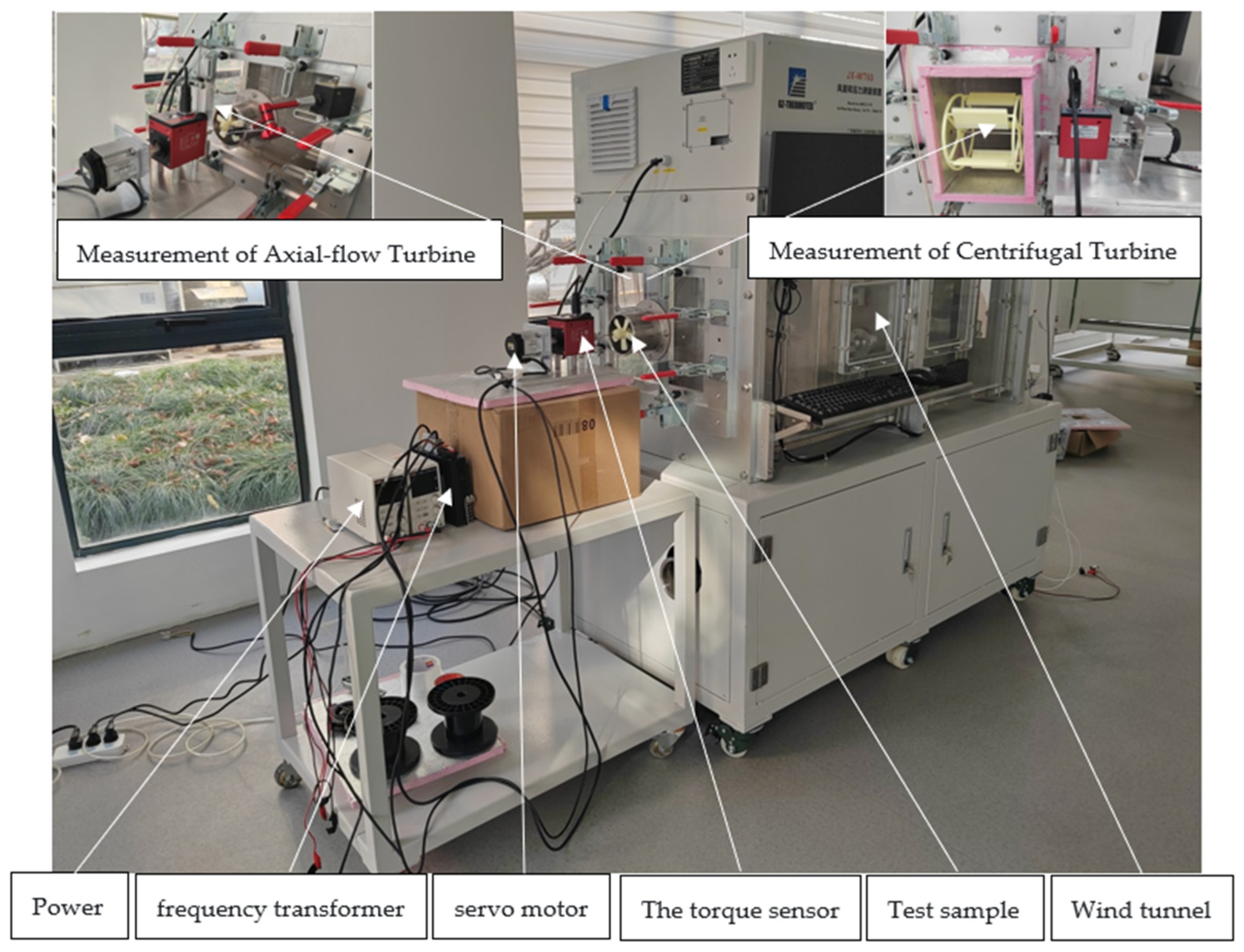
The entire test system is mainly composed of three parts: the wind tunnel platform, the external driving equipment, and the test impeller. The specific composition is shown in Figure 15 below, and the equipment models are shown in

Table 8. Model numbers of wind tunnel equipment.

No.	Equipment	Version	Quantity
1	Power	6PS6005D	2
2	frequency transformer	DB100-75	1
3	servo motor	DB60-00630A-A-R	1
4	The torque sensor	DYN-200	1
5	Wind tunnel	JX-WT60	1

. The schematic diagram of the internal structure and operating principle of the wind tunnel is also shown in Figure 16 below, from which we can clearly understand the airflow path. The airflow enters the wind tunnel cavity under the action of the auxiliary fan. Upon entering the cavity, the airflow first undergoes rectification through the first grille, which ensures uniform distribution of the airflow before entering the nozzle. After the airflow passes through the nozzle, it also passes through the second grille for rectification again. This second grille further ensures that the airflow is in a uniform state before reaching the tested specimen, thereby effectively improving the accuracy of the data measured by the pressure sensor. In addition, the back pressure in the cavity can be flexibly controlled by adjusting the number and diameter of the nozzles and the rotation speed of the auxiliary fan. During the test process, it is necessary to accurately record several key data, including the pressure rises Δp1 of the tested specimen, the pressure difference Δp2, the atmospheric pressure Patm, the dry-bulb temperature T1, the wet-bulb temperature T2, the ambient humidity Hatm, the impeller rotation speed n, and the impeller torque T. These data will provide an important basis for subsequent analysis and research.

This paper divides the experiments on the model prototype into two types: constant rotation speed experiments and constant flow velocity experiments.

(1) Constant rotation speed experiments

In constant rotation speed experiments, the water turbine is driven by a servo motor. The rotation speed of the servo motor is precisely set to 250 rpm, and then the aerodynamic performance of the water turbine is carefully measured by adjusting the back pressure of the wind tunnel. In this process, the stable rotation speed provides good experimental conditions for this paper to study the influence of back pressure on the aerodynamic performance of the water turbine.

(2) Constant flow velocity experiments

Constant flow velocity experiments adopt different operation methods. In this paper, an anemometer is used to measure the flow velocity at the air outlet of the tooling in real time, and a series of adjustment measures are taken to ensure that the flow velocity remains constant. On this basis, the rotation speed of the water turbine is changed, and then the aerodynamic performance of the water turbine at different rotation speeds is measured. This experimental method helps us explore the influence of the change in rotation speed on the aerodynamic performance of the water turbine when the flow velocity remains unchanged.

The specific content of the experimental DOE (Design of Experiments) is shown in

Table 9. DOE design parameters of the axial−flow turbine and centrifugal turbine.

No.	Fix Speed		Fix Inflow
Axial-Flow Turbine	Speed [rpm]	Air Flow [m3/h]	Speed [rpm]	Velocity [m/s]
1	250	6.40	103	2
2	250	16.80	207	2
3	250	30.50	311	2
4	250	47.30	415	2
5	250	60.40	519	2
6	250	69.70	623	2
7	250	80.50	726	2
8	250	91.00	830	2
9			1038	2
10			1246	2
11			1453	2
12			1661	2
13			1869	2
14			2076	2
15			2284	2
16			2492	2
17			2700	2
No.	Fix Speed		Fix Inflow
Centrifugal Turbine	Speed [rpm]	Air Flow [m3/h]	Speed [rpm]	Velocity [m/s]
1	250	13.10	69	2
2	250	21.30	138	2
3	250	30.60	208	2
4	250	41.10	277	2
5	250	51.40	346	2
6	250	68.10	415	2
7	250	77.50	485	2
8	250	87.30	554	2
9			692	2
10			831	2
11			969	2
12			1108	2
13			1246	2
14			1385	2
15			1523	2
16			1662	2
17			1800	2
18			1939	2

below:

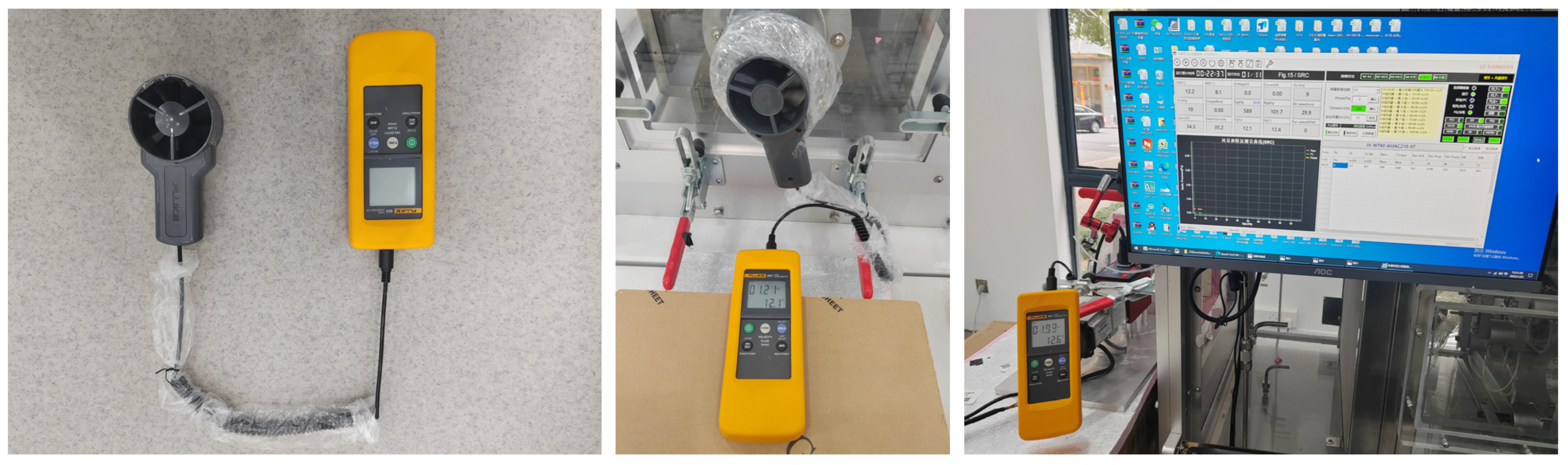
Figure 17 shows the specific process of wind speed measurement. In this measurement, the model 925 anemometer produced by FLUKE Company is selected. To ensure the accuracy of the measurement results, this device is carefully placed at the air outlet of the tooling, so that the airflow can enter the sensor vertically. At the same time, the interface between the sensor and the tooling is sealed to prevent interference from air leakage on the measurement results.

6.4. Verification of Numerical Simulation Results

After the multi-island genetic algorithm successfully finds the optimal solution, according to the setting schemes of constant rotation speed and constant flow velocity, this paper conducts steady-state CFD simulation calculations of the full flow passage for the water turbine data corresponding to the optimal solution. The following figures intuitively show the comparison between the simulation calculation results and the experimental test data.

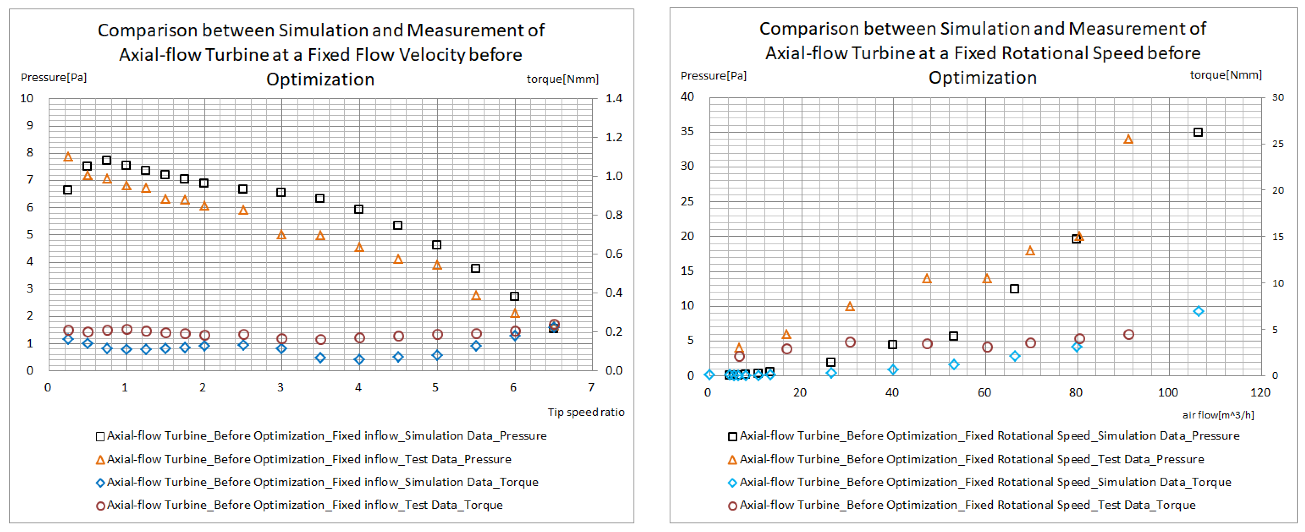
Figure 18 and Figure 19 detail the comparison between the simulation data and the experimental data of the axial-flow water turbine and the centrifugal water turbine before optimization. In the test of the axial-flow water turbine using the constant flow velocity measurement method, it can be seen from the data comparison results that the experimental results and the simulation data are highly consistent in the changing trends of the water turbine pressure (head) and the water turbine torque. However, the pressure presented by the simulation data is generally higher than the experimental test results. There are mainly two reasons for this phenomenon: firstly, the unevenness around the gap between the impeller and the pipeline leads to leakage; secondly, there is a certain deviation between the 3D printed sample and the theoretical 3D model, and the data of the simulation calculation strictly follow the theoretical values in terms of boundary conditions and dimensional shapes. When the tip speed ratio is 3, both the measured pressure data and the simulated pressure data show an obvious inflection point, and at this time, the pressure difference between the two reaches the maximum, about 1.5 Pa. In the area where the tip speed ratio is greater than 3, the pressure rise slope is large, and the pressure rises rapidly; while in the area where the tip speed ratio is less than 3, the pressure rise slope is small, and the pressure rises slowly. This is mainly because as the tip speed ratio (that is, the rotation speed of the water turbine) increases, the backflow phenomenon at the tip part of the impeller blades decreases, thereby improving the efficiency of the water turbine; when the tip speed ratio is small, the pressure difference between the upstream and downstream of the water turbine is large, and the air backflow phenomenon is significant, resulting in a relatively slow change in the pressure between the upstream and downstream of the water turbine. From the comparison of the torque data, the simulation data and the measured data are also consistent in the changing trend and order of magnitude, but the measured data are generally larger than the simulation data. This is mainly because, during the torque measurement process, the friction coefficients of components such as the bearing, torque sensor, and bearing chamber impact the measurement results, resulting in a larger measured torque value.

When the constant flow velocity measurement method is adopted, the changing trends of the simulation data and the test data in terms of pressure and torque remain consistent. Similar to the situation of the constant flow velocity measurement method, the measured values of the torque are generally larger than the simulated values, and the main reason is also the influence of the friction coefficients of components such as the bearing, the torque sensor, and the bearing chamber, which makes the measured torque value larger. However, as the flow rate increases, the increase in the torque of the water turbine exceeds the increase in torque caused by the friction coefficient. After the flow rate reaches 60 m³/h, the simulation data and the measured data have a high degree of coincidence. Before the flow rate is less than 60 m³/h, the deviation between the measured value and the simulated value of the pressure is large, while after the flow rate reaches 60 m³/h, the coincidence degree of the two is significantly improved. This may be because when the airflow in the wind tunnel cavity is small, the sensor is installed on the wall surface of the cavity, and the influence of the boundary layer leads to deviations in data collection.

When the centrifugal water turbine is measured by the constant flow velocity method, the simulation data and the measured data have a high degree of coincidence in terms of pressure and torque. In the case of the constant rotation speed measurement, the overall coincidence effect of the pressure and torque is good, but there is still a certain deviation in the torque. Specifically, after the wind speed reaches 2 m/s, the coincidence degree of the two is significantly improved; when the wind speed is lower than 2 m/s, the deviation is more obvious, and the lower the wind speed is, the greater the deviation will be.

The main reason for this phenomenon is that the rotation speed of the water turbine is set at a relatively low 250 rpm. When the wind speed is low, the friction factors generated by the bearing friction, the torque sensor, the bearing chamber, etc., account for a relatively large proportion of the measurement and cannot be ignored, increasing the measured value. However, as the wind speed continues to increase, the proportion of these friction factors gradually decreases, making the simulation data and the measured data gradually tend to be consistent.

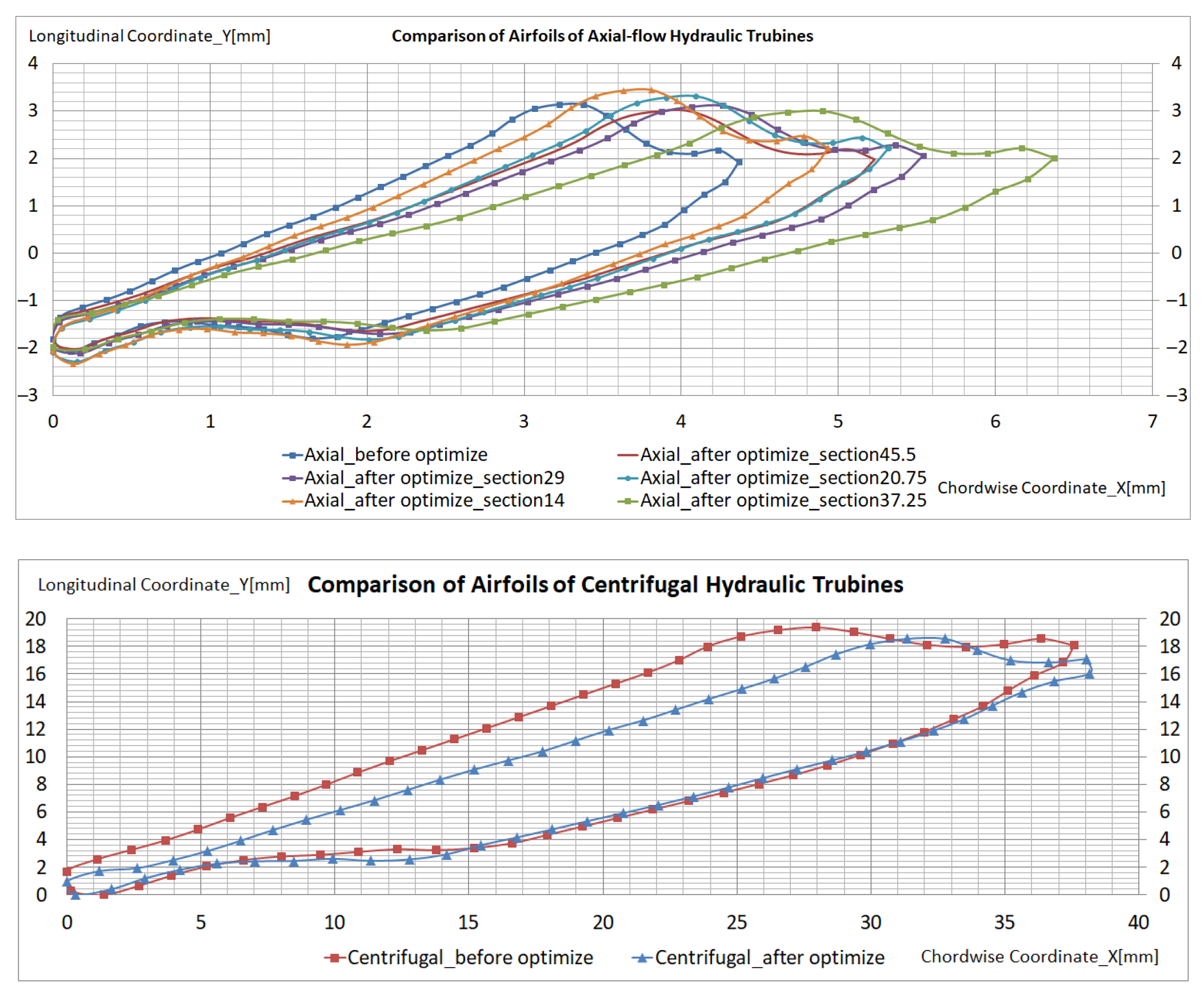
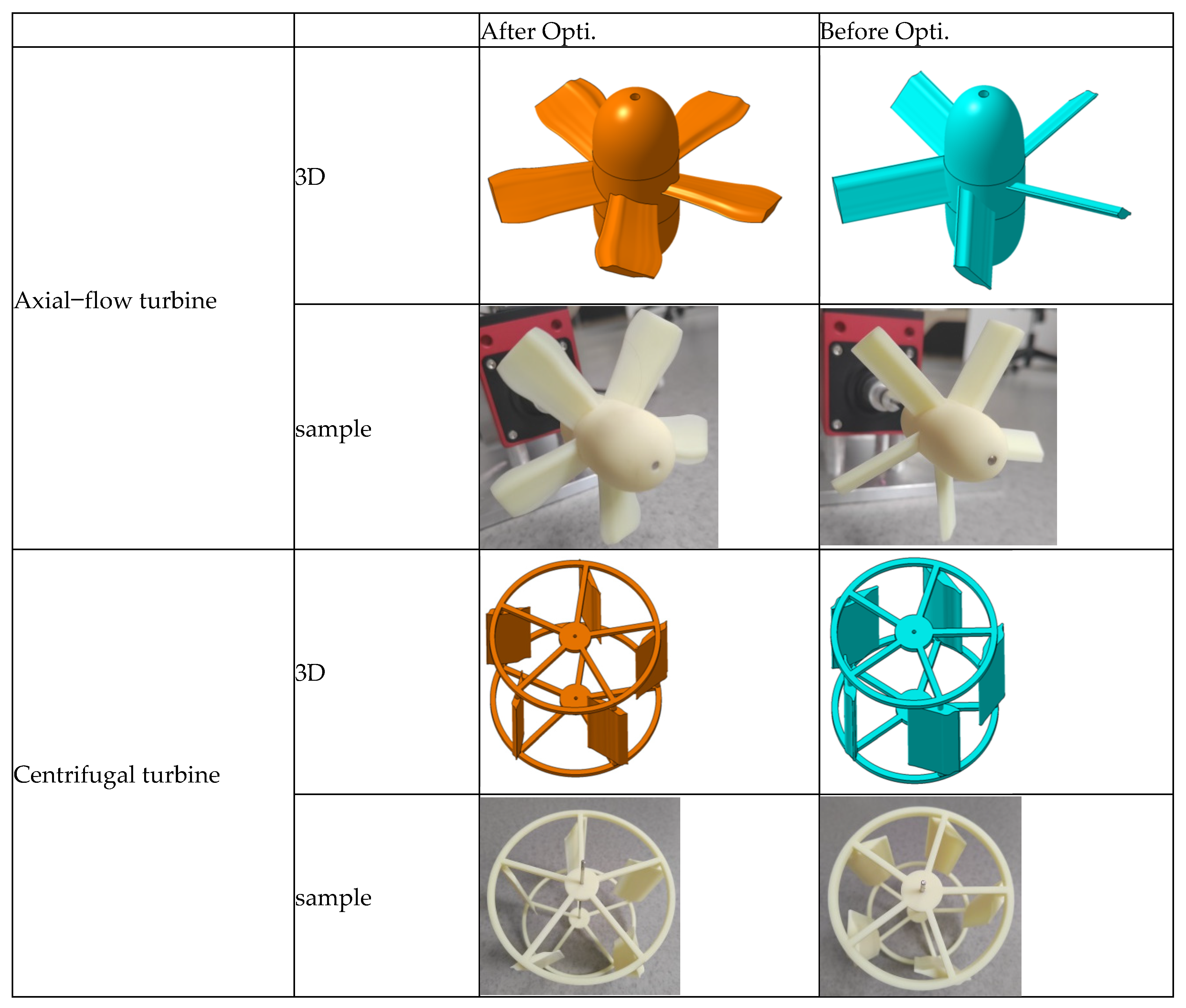
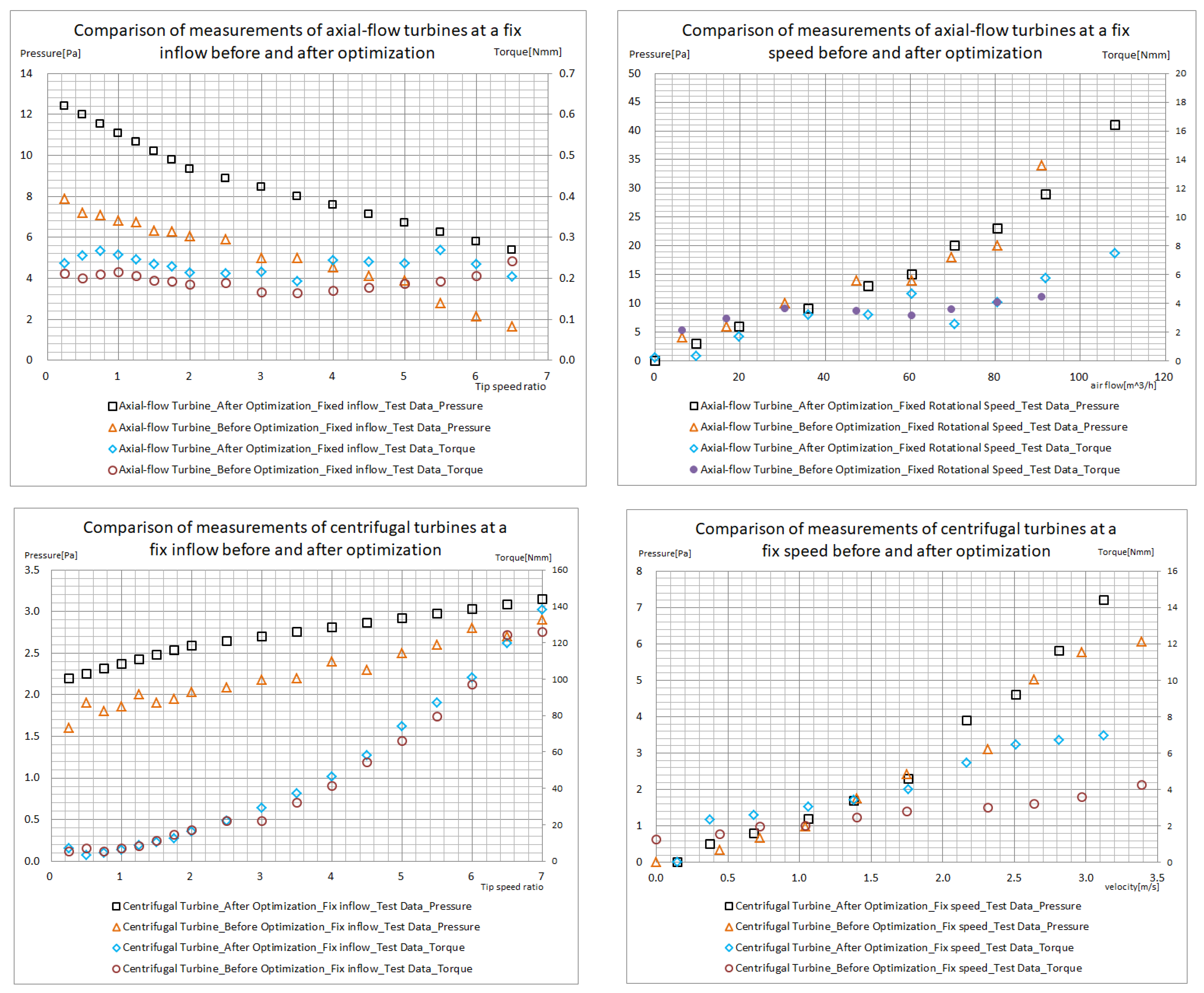
Figure 20 presents the comparison of the measured data of the axial-flow water turbine and the centrifugal water turbine before and after optimization. Through the comparative analysis of the simulation data and the measured data before optimization, we find that the simulation data can provide valuable references for the optimization calculation. Due to the limited length of this article, not all the data are presented.

It is not difficult to see from the measured data before and after optimization that, whether for the axial-flow water turbine or the centrifugal water turbine, the performance data after optimization are significantly better than those before optimization. In the constant flow velocity measurement mode, compared with that before optimization, the pressure of the optimized axial-flow water turbine can be increased by 55% at most, and the torque can be increased by 40% at most; the pressure of the optimized centrifugal water turbine can be increased by 60% at most, compared to that before optimization, and the torque can be increased by 12.5% at most.

When measured at a constant rotation speed, the pressure of the optimized axial-flow water turbine is at most 5 Pa higher than that before optimization, but the increase in torque is not significant. When the flow rate reaches 80 m³/h, the torques before and after optimization tend to be at a similar level. This may be because the axial-flow water turbine before optimization adopted the design of equal chord length and large angle of attack, making its starting torque relatively large. For the centrifugal water turbine, the pressure after optimization is slightly higher than that before optimization, but it is not as obvious as that in the constant flow velocity measurement, with an average increase of only about 0.2 Pa. However, the increase in torque is more significant, which can reach up to 1.6 N·mm at most.

Based on these measured data, this paper can conclude that using the shape function perturbation method and the characteristic parameter description method to establish the water turbine model, and using the multi-island genetic algorithm for optimization calculation, can effectively find a better solution, thus improving the performance of the water turbine.

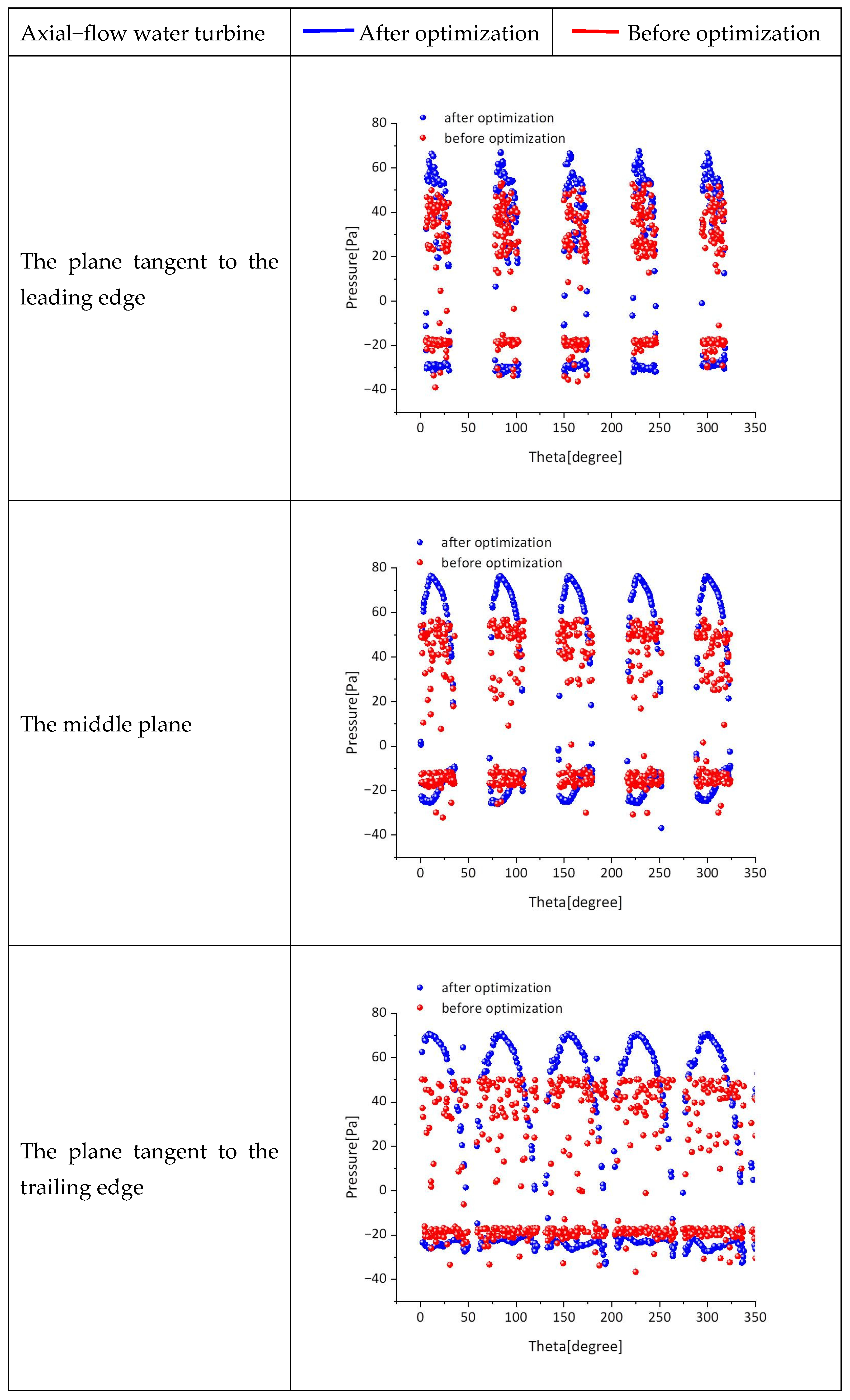
In this paper, three end faces are selected, as shown in Figure 21 and Figure 22 below. They are, respectively, the end face tangent to the leading edge of the axial-flow water turbine, the end face in the middle of the water turbine, and the end face tangent to the trailing edge. The purpose of selecting these three sections is to carefully observe the distribution of the pulsating pressure inside the flow field in terms of space and time during the flow of water.

(1) The plane tangent to the leading edge

On the plane tangent to the leading edge, both the pressure distribution range and the pressure value of the optimized axial-flow water turbine are greater than those before optimization. In the optimized water turbine, there is only a small negative pressure area at the blade tip, while in the water turbine before optimization, there is a negative pressure area in the region of 30–100%. Combined with the pressure distribution curve of this plane in the circumferential direction, this conclusion can also be verified. The positive pressure area of the curve of the optimized water turbine is larger and wider, and the maximum difference in positive pressure can reach 3 Pa; the negative pressure area is significantly smaller than that of the water turbine before optimization, and the maximum difference in negative pressure is 5 Pa. The main reason is that the installation angle of the water turbine before optimization is larger than that after optimization. When the end face is selected at the same position, part of the structure of the water turbine before optimization is exposed outside the end face, which leads to a larger negative pressure area and value compared with those after optimization.

(2) The middle plane

On the middle plane, the overall pressure intensity of the optimized axial-flow water turbine is significantly higher than that before optimization. From the pressure distribution curve of this area, it can be seen that the positive pressure of the optimized water turbine is 4 Pa greater than that before optimization, and the negative pressure is 6 Pa greater. It can be inferred from this that the optimized water turbine does significantly more work in the middle area than before optimization.

(3) The plane tangent to the trailing edge

The situation of the plane tangent to the trailing edge is similar to that of the middle plane. The overall pressure intensity of the optimized axial-flow water turbine is also greater than that before optimization. From the pressure distribution curve of this end face, it is known that the positive pressure of the optimized water turbine is 2 Pa greater than that before optimization, and the negative pressure is 10 Pa greater.

Based on the pressure diagrams of these three end faces, we can preliminarily determine that this optimization algorithm is indeed effective.

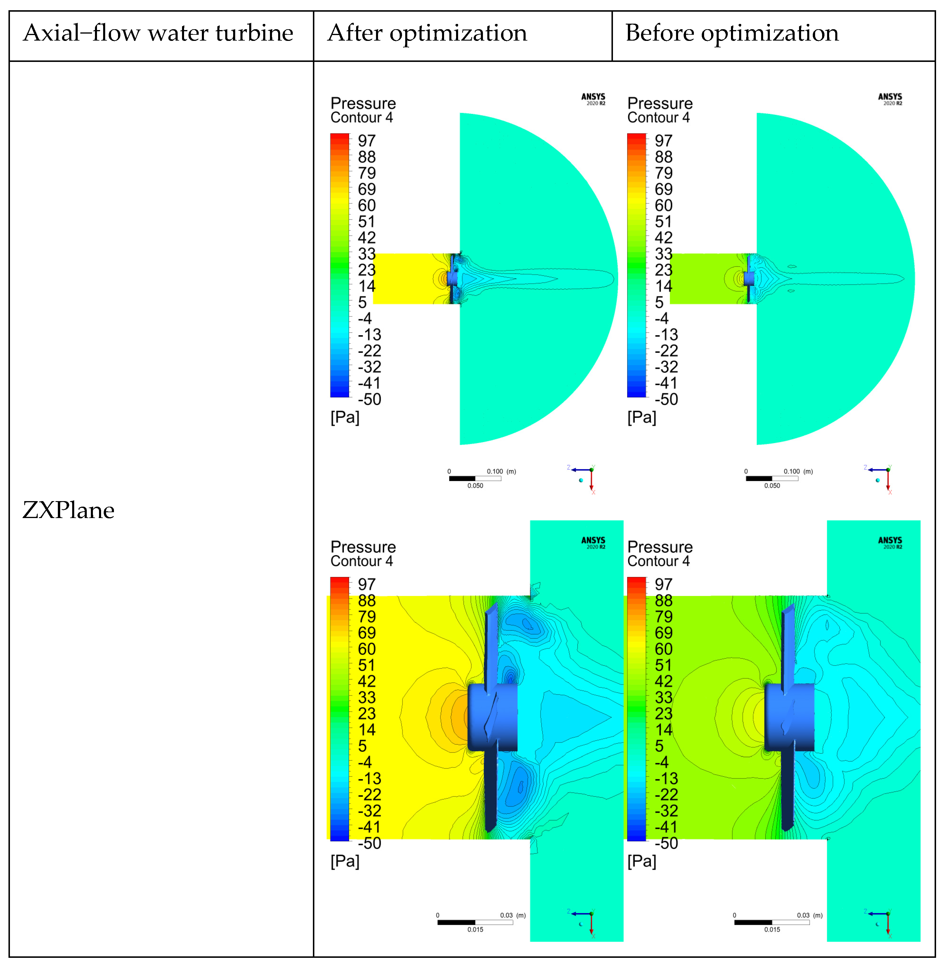
In this paper, the pressure nephogram of the ZX plane is intercepted, as shown in Figure 23 specifically. Since the pressure nephogram of the ZY plane is consistent with that of the ZX plane, to avoid content redundancy, the pressure nephogram of the ZY plane is not shown in this paper.

It can be observed from the intercepted pressure nephogram of the ZX plane that the pressure of the optimized axial-flow water turbine in its upstream region is higher than that before optimization, while the pressure in the downstream region is lower than that before optimization. Through data comparison, the pressure difference before and after the optimized water turbine is about 10 Pa, while the pressure difference before and after the water turbine before the optimization is about 5 Pa. Based on this, we can infer that the optimized water turbine has a stronger work capacity.

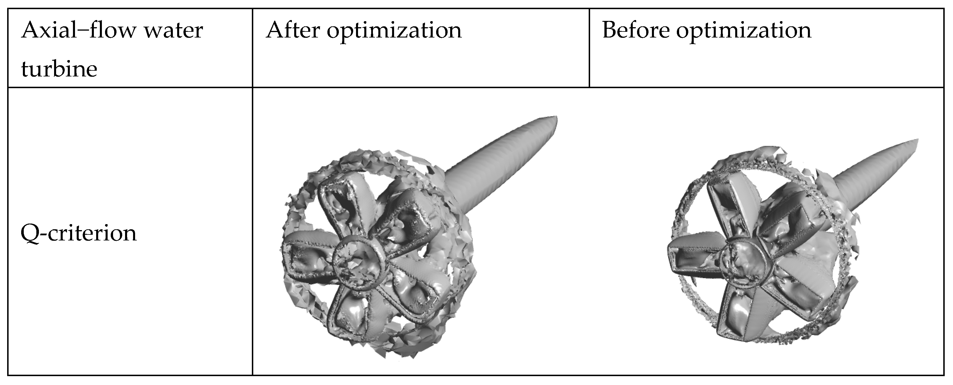
However, a phenomenon worthy of attention occurs at the blade tip part. The vortices generated by the optimized water turbine are larger than those before optimization. This situation may have an adverse effect on the noise level and lead to worse noise conditions. Specific content about the noise is introduced in detail in the next chapter. Combining with the Q-criterion of the vortex field, as shown in Figure 24 below, the Q-criterion is based on the velocity gradient tensor ${\mathrm{u}}_{\mathrm{i},\mathrm{j}}$ of the flow field and decomposes it into a symmetric part ${\mathrm{S}}_{\mathrm{i},\mathrm{j}}$ (strain rate tensor) and an antisymmetric part ${\mathrm{\omega }}_{\mathrm{i},\mathrm{j}}$ (rotation rate tensor). Among them, $S_{i,j}={\displaystyle \frac{1}{2}}\left(u_{i,j}+u_{j,i}\right)$, ${\omega }_{i,j}={\displaystyle \frac{1}{2}}\left(u_{i,j}-u_{j,i}\right)$. The Q value is defined as $Q={\displaystyle \frac{1}{2}}\left({\left|{\omega }_{i,j}\right|}^2-{\left|S_{i,j}\right|}^2\right)$, which measures the relative intensity of rotation and strain in the flow field. When Q > 0, the rotation effect in the flow field is dominant, and there may be vortex structures; when Q < 0, the strain effect is dominant. It can be found from the Q-criterion diagram that the intensity and area of the vortices of the optimized water turbine are larger than those before optimization, and the minimum value of the Q value is 0.01. Therefore, the main factor of the vortices in the flow field is caused by rotation.

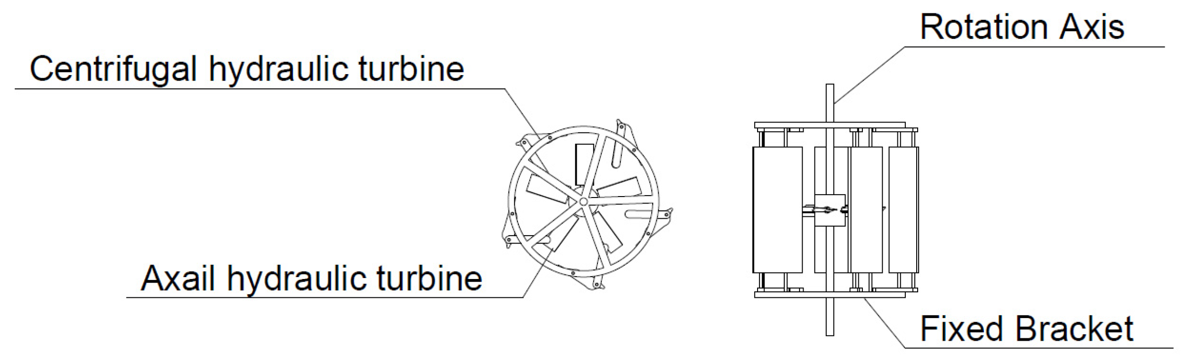
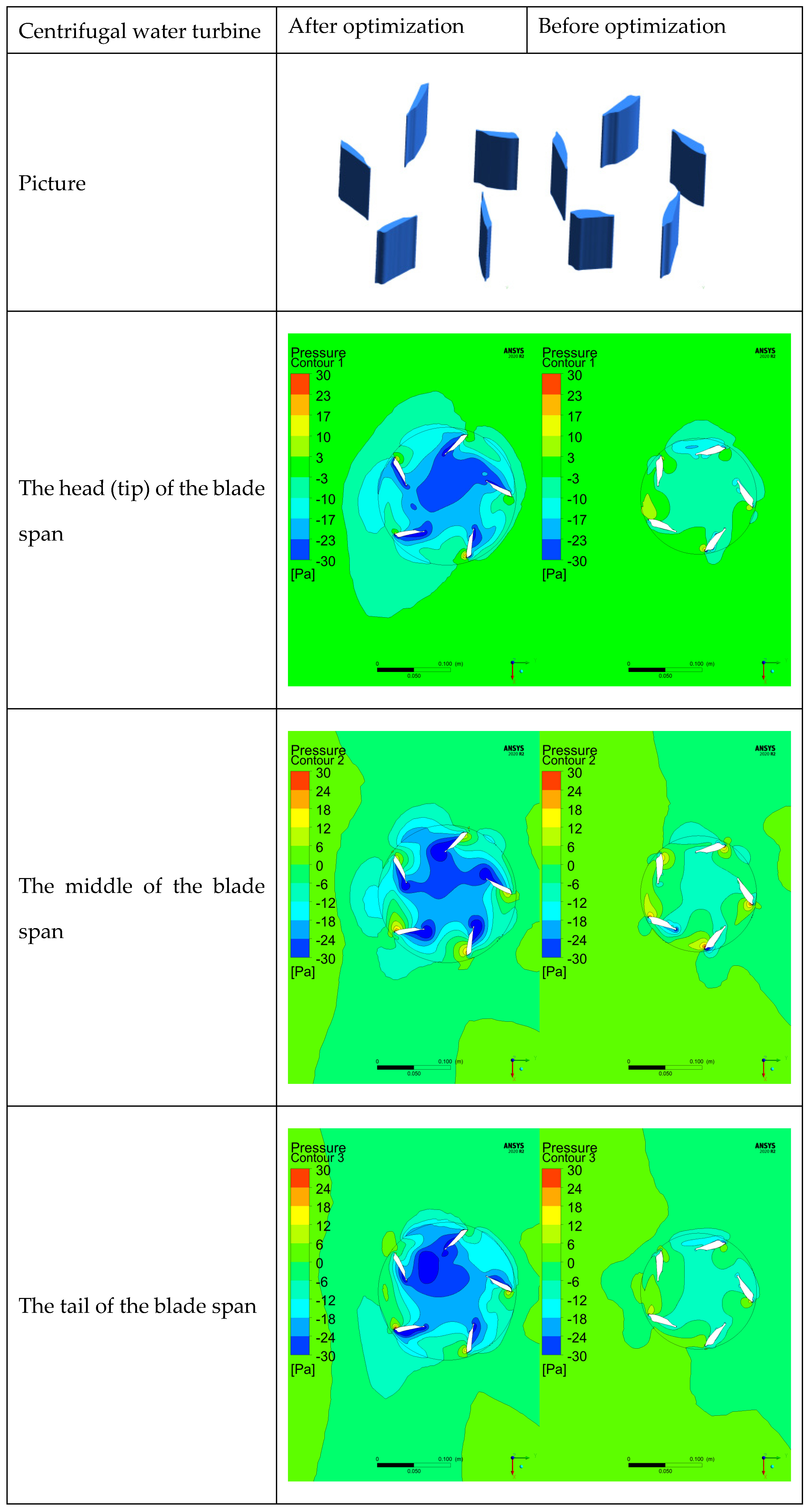
Similar to the treatment of the axial-flow turbine, in this paper, three planes are also intercepted for the centrifugal turbine, namely the head (tip) of the blade span, the middle of the blade span, and the tail of the blade span. From the pressure contour maps of these three planes (Figure 25), it can be found that the pressure differences between the front (pressure side) and the rear (suction side) of the optimized turbine blades are all greater than those before optimization. In a centrifugal turbine, the airfoil uses lift to push the blades to move, thereby realizing the rotation of the turbine. The pressure difference between the front and rear of the blade surface is the key parameter for generating lift.

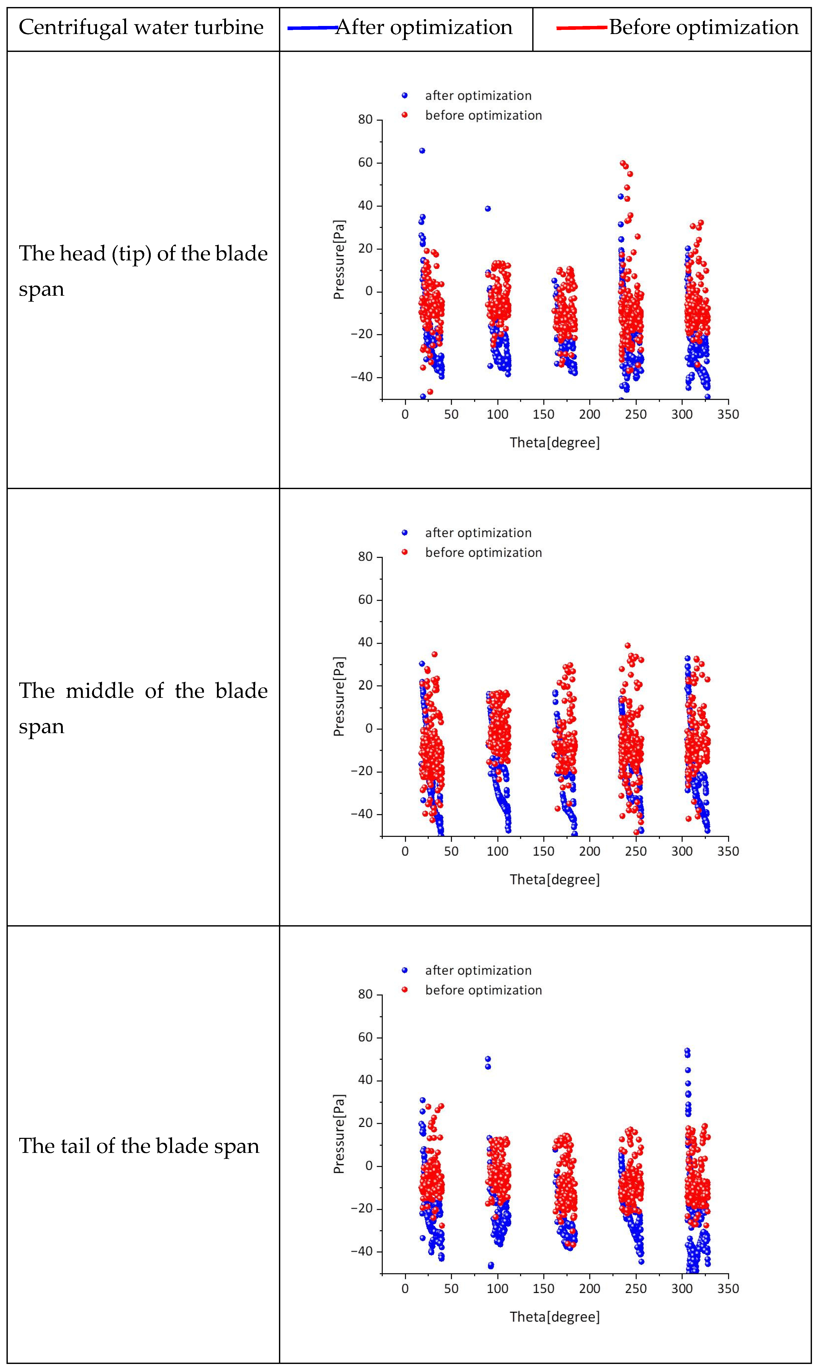
According to the pressure curve (Figure 26), the maximum pressure differences between the front and rear of the blades on the three planes of the optimized turbine are 85 Pa, 70 Pa, and 58 Pa respectively, while the corresponding maximum pressure differences before optimization are 70 Pa, 50 Pa, and 39 Pa respectively. It can be seen that the working capacity of the optimized turbine is significantly higher than that before optimization.

In addition, the distributions of the high-pressure and low-pressure peaks of the five blades of the centrifugal turbine are not as uniform as those of the axial-flow turbine. This is mainly due to the differences in the fluid flow patterns during the operation of the two types of turbines. When the axial-flow turbine is in operation, the fluid can uniformly pass through the five blades from the upstream. However, when the centrifugal turbine is in operation, the fluid passes through the five blades in sequence, and the position of each blade relative to the incoming flow is different. At the same time, the wake generated by the front blades will also affect the wake of the rear blades, resulting in non-uniform pressure distribution.

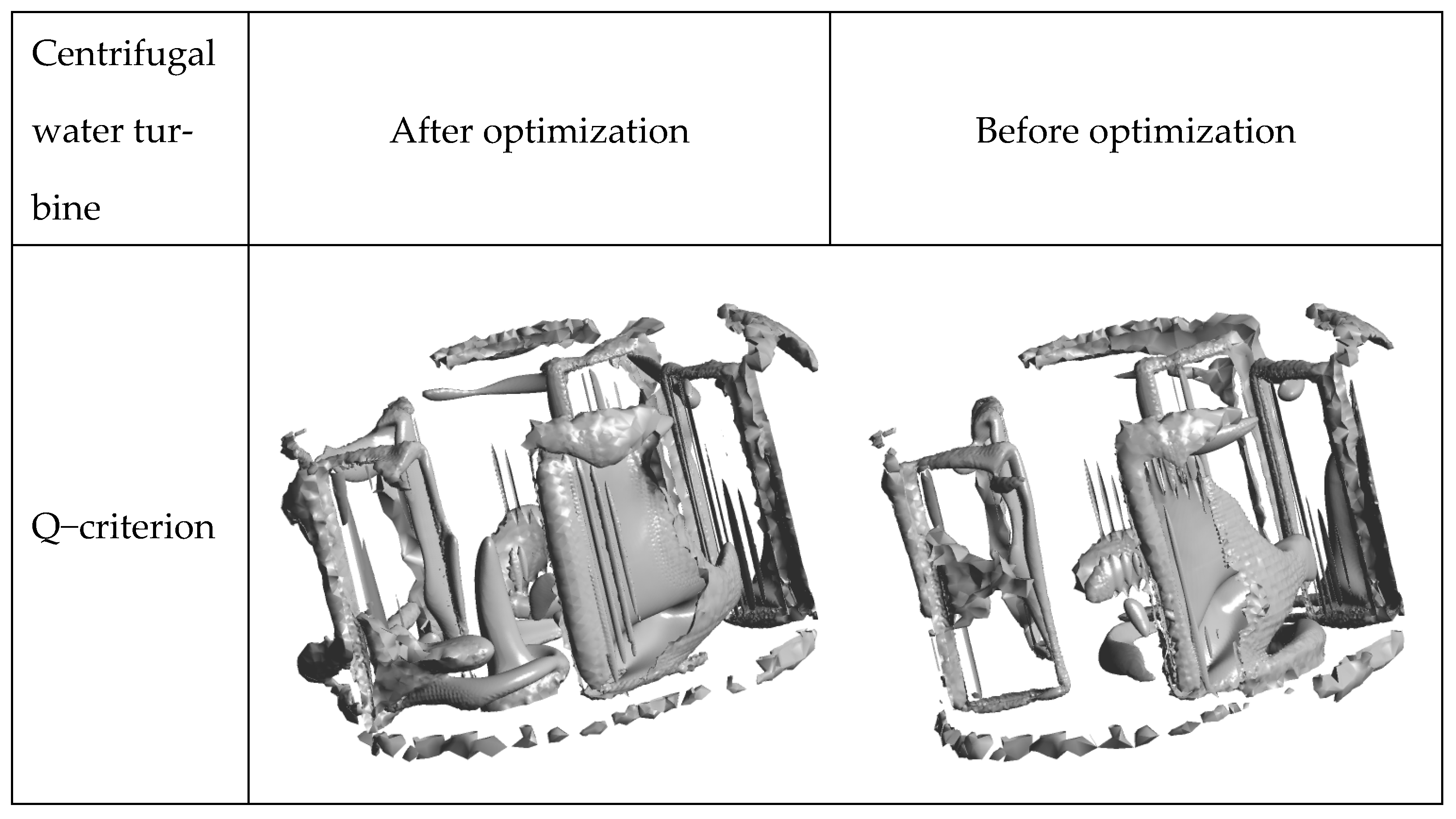
Figure 27 below shows the Q-criterion image of the centrifugal water turbine. It can be seen from the figure that the result is similar to that of the axial-flow fan. For the optimized centrifugal water turbine, the intensity of its vortex field is significantly greater than that before optimization.

In the flow field, the main cause of vortex formation is rotation. In the case of the centrifugal water turbine, this situation mainly occurs because the pressure difference between the front and back of the blades of the optimized water turbine increases, enhancing the work capacity of the water turbine. This change leads to an increase in the degree of rotation of the flow field and thus increases the intensity of the vortices.

7. Discussion

7.1. Axial-Flow Turbine Performance Analysis

The optimization of the axial-flow turbine via the multi-island genetic algorithm (MIGA) demonstrates significant improvements in hydrodynamic performance. Post-optimization, the pressure rise and torque increase by up to 55% and 40%, respectively, under constant flow velocity conditions (Figure 18). This enhancement is primarily attributed to the adjusted blade installation angles (reduced by 4.81–8.01° across sections) and increased camber angles (15°→17.73–23.68°), which optimize the flow incidence angle and enhance lift generation. The pressure contour plots (Figure 21) reveal a reduced negative pressure zone at the blade tip post-optimization, indicating mitigated tip vortex separation and improved flow attachment. However, the intensified vortex structures at the blade tip (Figure 24), characterized by a Q-criterion value of 1.5 × 10⁻⁶, suggest potential increases in noise and structural loading, and warrant further investigation in future studies.

Notably, the constant rotation speed experiments show limited torque improvement (Figure 18), likely due to the pre-optimization design’s large attack angle, favoring high starting torque. The simulation–experiment discrepancy in pressure (Figure 18) stems from impeller-pipeline gap leakage and 3D printing tolerances, highlighting the need for precise manufacturing in practical applications.

7.2. Centrifugal Turbine Performance Analysis

For the centrifugal turbine, optimization yields more pronounced torque enhancements (up to 12.5%) compared to pressure rises (average +0.2 Pa) under constant rotation speed conditions (Figure 19). This is attributed to the increased blade thickness coefficient (1.1→1.25) and optimized camber angle (20°→17.46°), which strengthens lift-driven rotation while maintaining structural integrity. The pressure difference between the blade’s pressure and suction sides increases by 21.4–56.4% across spanwise sections (Figure 25), directly boosting power output.

However, the non-uniform pressure distribution among the five blades (Figure 25) arises from sequential fluid passage and wake interactions, a characteristic challenge of centrifugal designs. The intensified vortex fields observed post-optimization (Figure 26), although indicative of enhanced rotational energy, may exacerbate flow-induced vibrations. Future work should explore sweep angles or slot designs to mitigate wake interference and improve load uniformity.

7.3. Comparative Insights and Optimization Efficacy

The MIGA effectively balances multi-objective constraints, with the axial-flow turbine prioritizing pressure rise and the centrifugal turbine emphasizing torque efficiency. The axial design’s uniform flow passage facilitates consistent performance across sections, while the centrifugal design’s radial flow path offers higher energy capture at the expense of flow uniformity. Both designs validate the efficacy of combining shape function perturbation and genetic algorithms, with the former enabling precise geometric control and the latter ensuring global optimization.

Notably, the axial-flow turbine’s superior pressure performance makes it suitable for high-head applications, whereas the centrifugal turbine’s torque efficiency is ideal for low-speed, high-torque scenarios. The trade-off between vortex intensity and energy efficiency underscores the need for multi-physics optimization, integrating aerodynamics, structural mechanics, and acoustics.

7.4. Limitations and Future Directions

This study assumes steady tidal and wave flows, which may not fully replicate real-world unsteady marine conditions. Additionally, the neglect of multiphase flow effects (e.g., air–water interactions) introduces uncertainties in practical marine deployments. Future research should incorporate real-time wave-tide coupling models and experimental validation under turbulent flow conditions. Advanced materials (e.g., composites) and active flow control techniques (e.g., plasma actuators) could further mitigate vortex-induced losses and enhance durability.

In summary, the MIGA-based optimization provides a robust framework for tidal turbine design, offering clear pathways for performance enhancement in both axial-flow and centrifugal configurations.

8. Conclusions

In the field of water turbine modeling and optimization, to accurately construct the water turbine model, this paper innovatively adopts the shape function perturbation method and the characteristic parameter description method. These two methods complement each other and depict the characteristics of the water turbine from different dimensions, laying a solid foundation for the subsequent optimization analysis.

8.1. Conclusion on Axial-Flow Turbine

In this study, the optimized design of axial-flow turbines achieved systematic performance improvement through the organic integration of analytical design methods and optimization design approaches. Based on blade element theory, three-dimensional flow effects were introduced, and parametric modeling of key parameters such as blade number, installation angle, camber angle, and hub ratio was conducted to construct an airfoil model with both controllability and completeness. Through the deep integration of CATIA 3D modeling and the Isight platform, combined with the global optimization capability of the multi-island genetic algorithm (MIGA), the turbine’s torque and energy capture coefficient were significantly enhanced.

During the optimization process, adjusting the chord length coefficient, thickness coefficient, and installation angles of each section ensured the smoothness of the airfoil contour lines, effectively avoiding the generation of computational singular points. The multi-island genetic algorithm suppressed the convergence to local optimal solutions and significantly improved global search efficiency by dividing independent “island” populations and implementing periodic individual migration. Simulation and experimental verification showed that the optimized axial-flow turbine achieved a maximum pressure increase of 5 Pa and a maximum torque increase of 0.8 N·mm, with particularly significant performance improvements under constant flow velocity conditions. However, the increased vortex intensity in the blade tip region may lead to noise issues, which require further optimization in subsequent research.

8.2. Conclusions on Centrifugal Turbine

For centrifugal turbines, this study adopted an equal airfoil design strategy and achieved automatic airfoil optimization through parametric adjustments of installation angle, camber angle, chord length coefficient, and thickness coefficient, combined with a multi-island genetic algorithm. Using the collaborative workflow of CATIA and Isight, full-process automation from 3D modeling and mesh generation to CFD simulation was completed, significantly shortening the design cycle.

The optimization results showed significant improvements in the torque and energy capture coefficient of centrifugal turbines: under constant flow velocity conditions, the maximum torque increase was 10 N·mm, and the average pressure increase was 0.2 Pa; under constant rotational speed conditions, the maximum torque increase was 1.6 N·mm. Pressure contour plots indicated a significant increase in the pressure difference across the blades after optimization, enhancing work capacity. However, due to fluid flow sequence and wake interference, the uniformity of blade pressure distribution was lower than that of axial-flow turbines. Q-criterion analysis showed increased vortex field intensity after optimization, reflecting enhanced flow field rotation effects, which were consistent with the trend of improved work capacity.

In summary, the optimization studies of both turbines demonstrated that parametric modeling based on shape function perturbation methods and characteristic parameter description, combined with the global optimization strategy of the multi-island genetic algorithm, is an effective approach to unlocking the performance potential of turbines. Axial-flow turbines exhibit significant advantages in handling three-dimensional flow effects and multi-section parameter optimization, while centrifugal turbines achieve efficient optimization through single-airfoil parameter adjustment. Future research can further integrate noise control and structural strength analysis to promote the engineering application of turbine optimization design.