Dynamic Characteristics of a Digital Hydraulic Drive System for an Emergency Drainage Pump Under Alternating Loads

Abstract

With the frequent occurrence of global floods, the demand for emergency rescue equipment has grown rapidly. The development and technological innovation of digital hydraulic drive systems (DHDSs) for emergency drainage pumps (EDPs) have become key to improving rescue efficiency. However, EDPs are prone to being affected by random and uncertain loads during operation. To achieve intelligent and efficient rescue operations, a DHDS suitable for EDPs was proposed. Firstly, the configuration and operation mode of the DHDS for EDPs were analyzed. Based on this, a multi-field coupling dynamic simulation platform for the DHDS was constructed. Secondly, the output characteristics of the system under alternating loads were simulated and analyzed. Finally, a test platform for the EDP DHDS was established, and the dynamic characteristics of the system under alternating loads were explored. The results show that as the load torque of the alternating loads increases, the amplitude of the pressure of the motor also increases, the output flow of the hydraulic-controlled proportional reversing valve (HCPRV) changes slightly, and the fluctuation range of the rotational speed of the motor increases. The fluctuation range of the pressure and the rotational speed of the motor are basically not affected by the frequency of alternating loads, but the fluctuation amplitude of the output flow of the HCPRV reduces with the increase in the frequency of alternating loads. This system can respond to changes in load relatively quickly under alternating loads and can return to a stable state in a short time. It has laudable anti-interference ability and output stability.

1. Introduction

In recent years, extreme weather has caused frequent global floods, seriously threatening life safety and causing significant economic losses. Traditional fixed drainage equipment struggles to meet the demands of rapid and convenient emergency rescue, while vehicle-mounted mobile drainage equipment is widely utilized because of its high mobility and flexibility. According to their driving modes, different types of vehicle-mounted mobile drainage equipment can be classified into electric drive types, internal combustion engine direct drive types, and hydraulic drive types. Among them, the hydraulic drive type has become a research hotspot because of its merits, such as its high power-to-weight ratio, safety, and reliability. However, traditional hydraulic-driven EDPs have problems such as complex systems, poor reliability, and low levels of intelligence in complex environments, and they are unable to respond efficiently to flood disasters. Therefore, it is crucial to develop a hydraulic-driven EDP set with a large flow that is safe, reliable, intelligent, and efficient.

To enhance the transmission efficiency of the EDP system and reduce the energy consumption of the pumps, Tian et al. [1] proposed a high-flow multi-condition pump structure which mainly consists of a main pump, an auxiliary pump, a suction chamber, and a slide valve. The pump uses the slide valve to achieve series and parallel operation. Wang et al. [2], aiming to improve the efficiency of the pump, optimized the impeller and diffuser of the pump using orthogonal arrays and the numerical simulation approach of computational fluid dynamics, effectively improving the hydraulic characteristics and operational stability of the pump. Rakibuzzaman et al. [3] used the Rayleigh–Plesset model to forecast cavitation and increased the average efficiency of the system by 4.32% by optimizing the shapes of the impeller and the pump casing. Cao et al. [4] used the MUSIG model to simulate and analyze the gas–liquid two-phase flow of an EDP and obtained the influence laws of different inlet gas volume fractions on the capability of the pump, as well as vortices in the impeller and guide vanes. Gong et al. [5] proposed a genetic algorithm coupled with successive approximation of head and water levels to optimize urban tidal drainage pumps in response to the mismatch problem of head and water levels in different time periods at pumping stations. Huang et al. [6] introduced a fault diagnosis approach which utilizes minimum entropy deconvolution–wavelet packet decomposition combined with a radial basis function neural network to tackle the issue of vibration signals from drainage pumps, which gradually diminish in intensity as they traverse a complex transmission pathway and ultimately become obscured by ambient noise. This method reduces the interference of ambient noise and highlights the characteristics of the fault signal. Ye et al. [7] took advantage of the good thermal conductivity, strong electromagnetic driving ability, and wide working temperature range of liquid metal to study a separated electromagnetic centrifugal pump, which effectively increases the output power of the centrifugal pump. Kushwaha et al. [8] compared the dynamic performance of hydraulic motor drive systems controlled by pumps, valves, and prime movers under various working conditions. Their study found that the sensitivity of valve-controlled motor drive systems is higher than that of other systems, and the overload of the load-sensitive pump control is smaller. Zhu et al. [9] constructed a convolutional neural network through a batch normalization strategy, which improved the recognition accuracy of typical faults in plunger pumps and achieved the automatic recognition of typical faults in axial plunger pumps. Tang et al. [10] proposed a deep model approach based on synchronous compressed wavelet transform and a Bayesian optimization algorithm to settle the problems of time-consuming parameter adjustment and limited characteristic information for a single signal in the fault diagnosis of hydraulic pumps. This method was effective at analyzing fault characteristic information and intelligently identifying common fault types. Chang et al. [11] developed an efficiency optimization approach for centrifugal pumps based on the energy conservation equation and non-dominated sorting genetic algorithms-II. The efficiency of the optimized model increases by 2.754%, the total energy loss is significantly reduced, and the internal flow is more stable. Tang et al. [12] developed a fault diagnosis approach for hydraulic pumps that integrates the capabilities of long short-term memory networks with convolutional neural networks. The approach has superior accuracy and stability in multiple types of fault identification tasks, with an average test accuracy rate reaching 99.53%. Wang et al. [13] analyzed the impact of an impeller with baffles and an interlaced arrangement on the internal flow field and radial force characteristics of a centrifugal pump, and proposed an improved impeller plan using baffles and an interlaced arrangement, providing a novel method for increasing the efficiency and stability of double-suction centrifugal pumps. Zhao et al. [14] implemented numerical modeling and conducted an empirical analysis on the performance changes in centrifugal pumps under different fluid viscosities. The results showed that the increase in fluid viscosity decreased the head and efficiency of the pump and shifted the optimal operating point of the pump to the left. Pang et al. [15] adjusted the operating frequency of a pump using a variable-frequency drive to ensure that the operating parameters of the pump met the requirements of sprinkler irrigation while avoiding unnecessary energy waste. Wang et al. [16] proposed a machine learning-based condition monitoring method for axial piston pumps. By evaluating the waveform similarity between the monitoring pressure-release signal of the pump and the real-time health reference signal, abnormal monitoring of the pump was achieved.

Digital hydraulics systems require high-frequency responses, high precision, and high environmental tolerance. Hydraulic drive systems integrated with digital hydraulics can enhance equipment reliability, reduce comprehensive costs, and lower maintenance difficulty [17]. Among these systems, the high-speed on/off valve (HSV), a typical digital hydraulic valve, has been extensively utilized in fields such as construction machinery and vehicle engineering due to its small throttling loss and strong anti-pollution ability. Gao et al. [18] compiled a review of the findings pertaining to the discrete voltage and pulse control mechanisms of single-HSV- and parallel-HSV-encoding schemes. They conducted an analysis and comparison of the respective strengths, weaknesses, and applicable domains for various HSV control methodologies. Yang et al. [19] developed a new type of HSV driven by dual-magnetic circuits, with the on/off response times of the HSV being adjusted by precisely regulating the duty cycle of the delay phase and the motion phase. Xu et al. [20] developed a novel recognition approach based on current derivatives, matching the feature points in the current derivative model with each switching state of the HSV. The results showed that the maximum recognition error of this recognition method was only 1.49%. Gao et al. [21] introduced a sliding mode control strategy based on an intelligence control allocation method, which not only significantly improved the position-tracking accuracy of digital valves but also reduced the overall switching frequency, thereby extending the service life of digital valve arrays. Huang et al. [22] introduced an optimization approach based on multi-objective optimization and evolutionary algorithms. Through the three-voltage control strategy, the coil parameters of the multi-coil integrated HSV were optimized. Kogler [23] designed a high-dynamic digital control mechanism for a constant-load hydraulic cylinder in order to improve the maximum dynamic response of the system. This control strategy achieved a robust dynamic response within the hydraulic system and mitigated the oscillations induced by the on/off processes of the digital valve. Gao [24] designed a pressure controller composed of differential PWMs, APDCs, and NACs, which were, respectively, used to improve the net flow resolution, balance the oil-filling and -discharging capacity at different working pressure points, and overcome parameter uncertainty. Experimental results indicate that the controller exhibits excellent tracking characteristics. Yang et al. [25] developed an HSV control strategy based on adaptive fuzzy PID and dead zone compensation, which can remarkably enhance the control accuracy of valve core displacement. Li et al. [26] introduced a time-delay compensation control strategy based on PWM, which significantly reduced the energy consumption and time delay of HSVs. Zhong et al. [27] proposed an optimization-based pre-excitation control algorithm, which optimized the opening and closing times of HSVs to 1.21 ms and 1.71 ms, with the final temperature rising to 40.9 °C. Zhong et al. [28] utilized a multi-objective optimization approach to obtain a high-precision equivalent magnetoresistance model for HSVs. The results indicated that the new HSV reduced the coil volume by 47.1% and simultaneously improved the dynamic performance. Compared with the aforementioned studies, the high-speed switching valve proposed in this research is controlled by a composite PWM signal, which can effectively reduce the opening and closing time and power consumption of the high-speed switching valve, ensuring better dynamic performance. The compound PWM not only ensures the complete opening and closing of the valve core but also shortens the opening lag time and closing lag time. As a result, the emergency drainage pump can respond more quickly to changes in load.

Existing EDPs mainly adopt traditional hydraulic drive systems, which have defects such as complex configurations, poor reliability, and a low degree of intelligence. They still face considerable challenges in applications in harsh environments with variable loads and external disturbances. To enhance the intelligence and reliability of the EDP system, a DHDS based on HSVs has replaced the traditional hydraulic system and has been applied to EDPs, helping to overcome the issue of the limited application of DHDSs in the field of EDPs. At the same time, it verified that the EDP with the DHDS could still maintain high stability under alternating loads.

This study studies a DHDS for EDPs, revealing the drive mechanism and dynamic response characteristics of the system under alternating loads. The main contributions are as follows:

(1)

A DHDS suitable for EDPs is introduced. This system adopts the energy transmission mode of hydraulic power source–hydraulic valve group–hydraulic motor–drainage pump. The HSV serves as the pilot control module for the proportional directional control valve, and a composite PWM signal is employed to drive and control its output flow, thereby enabling stepless speed adjustments for the hydraulic motor and enhancing the robustness and dynamic efficiency of drive system.

(2)

The mechanical–hydraulic multi-field coupling drive mechanism of a DHDS for EDPs is revealed. A multi-field coupling simulation platform and test platform are constructed, and the output characteristics and dynamic response characteristics of the system under alternating loads are clarified.

The remaining part of this article is arranged as follows: In Section 2, the composition structure and working principle of the DHDS for EDPs are analyzed. Mathematical modeling is carried out on the key components in the hydraulic valve control unit and the actuator unit, and an open-loop model of the system is established. In Section 3, a closed-loop model of the DHDS was established using the PID control algorithm, and PID parameter tuning was carried out. In Section 4, according to the alternating-load model, the dynamic response characteristics of the system under alternating loads are explored through simulation. In Section 5, a test platform for the DHDS for EDPs is established. The dynamic response characteristics of the system under alternating loads are measured, verifying the correctness of the theoretical research and simulation analysis in this paper. In Section 6, the main conclusions of the research are summarized.

2. DHDS Modeling

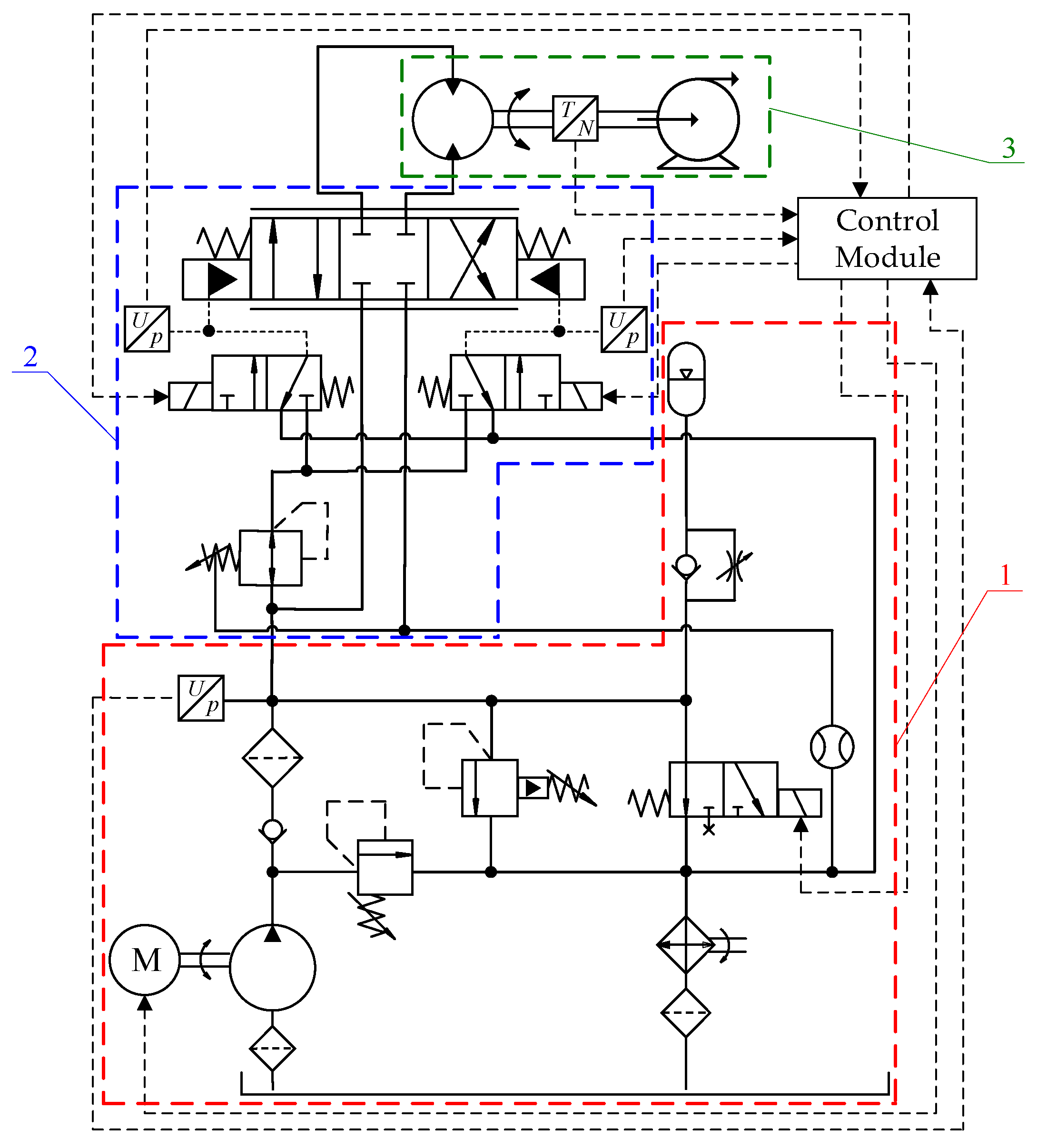
2.1. System Composition and Working Principle

The principle of the constructed DHDS for EDPs is depicted in Figure 1. The entire system mainly consists of the power unit, the hydraulic valve control unit, and the execution unit. Among them, two two-position three-way HSVs independently control the left and right hydraulic chamber-controlled proportional reversing valves (HCPRVs). By controlling the on/off state and on/off time of the HSV, the reversing movement and speed control of the hydraulic motor are achieved, and then the EDP is driven by the hydraulic motor. Since the direction of the EDP is fixed during normal operation, the hydraulic motor does not need to be involved in reverse rotation.

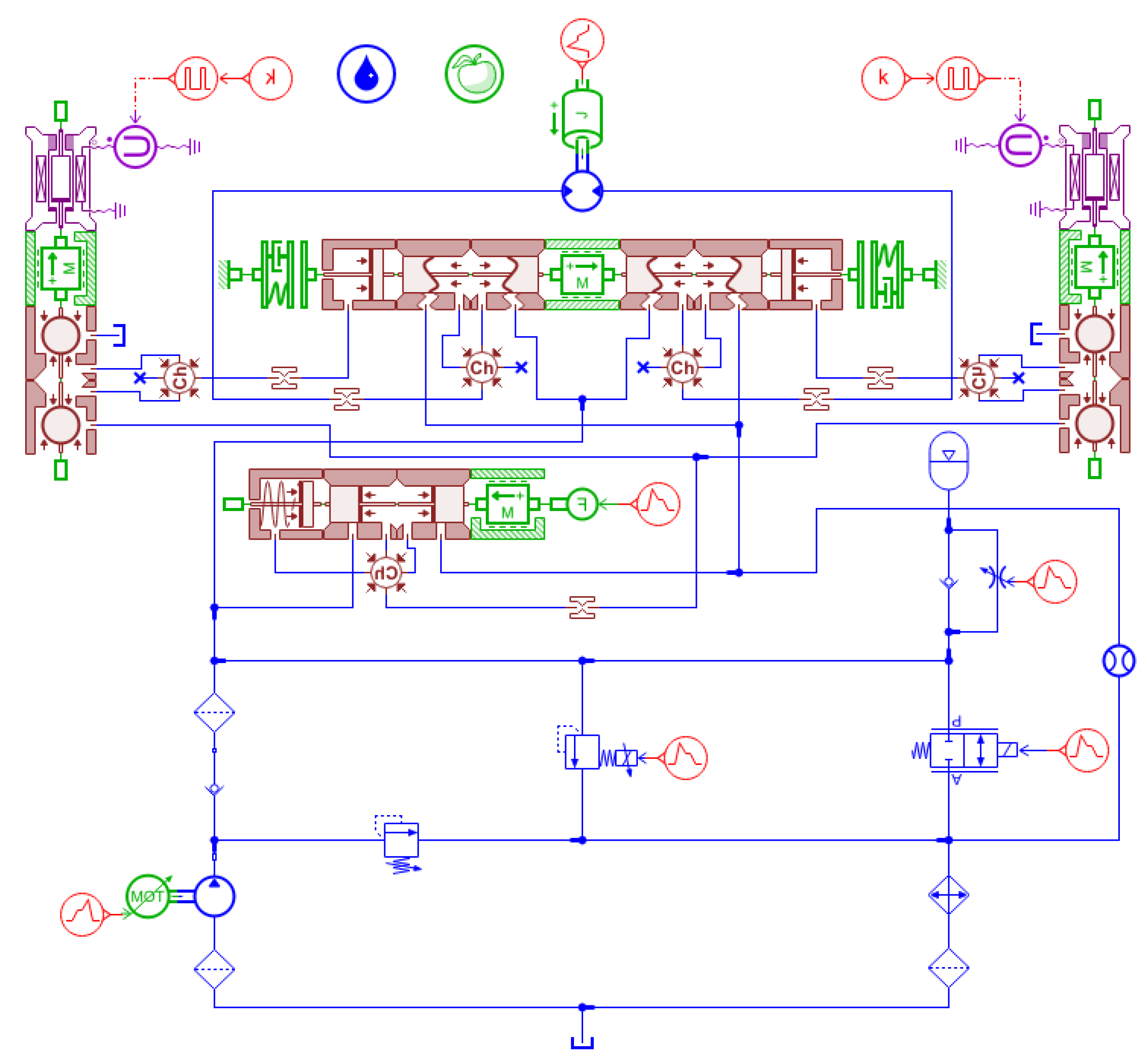
2.2. Modeling of the Hydraulic System

2.2.1. Model of the Power Unit

This paper constructs a power unit that can be used to adjust the output flow and working pressure of the entire DHDS. The principle of the power unit is shown in Figure 2. This power unit includes hydraulic pumps, servo motors, a direct-acting relief valve, a pilot-operated proportional relief valve, a solenoid directional control valve, an accumulator, coolers, and other hydraulic components.

For a pump, without considering its mechanical efficiency and leakage, the simplified mathematical model expression is as follows:

$$\left\{\begin{array}{l}{Q}_{\mathrm{pi}}={\displaystyle \frac{V_{\mathrm{p}}\cdot {\omega }_{\mathrm{p}}}{2\pi }}\times 60\\ T_{\mathrm{p}}=V_{\mathrm{p}}\cdot \left(p_{\mathrm{pj}}-p_{\mathrm{pi}}\right)\\ Q_{\mathrm{pj}}=-Q_{\mathrm{pi}}\end{array}\right.$$

(1)

where V_p represents the displacement of the pump; ω_p is the angular velocity of the drainage pump; p_pi represents the inlet pressure of the pump; p_pj represents the outlet pressure of the pump; Q_pi represents the oil-inlet flow of the pump; Q_pj represents the flow at the oil outlet of the pump; and T_p represents the input torque of the pump.

The accumulator is of vital importance in DHDSs. Reasonable configuration of the accumulator parameters can not only enhance the dynamic performance of the system but also reduce the noise level of the system during startup and operation [29]. When the oil enters the accumulator, the gas is compressed, its volume decreases, and the gas pressure rises. At this moment, the pressure in the air chamber is equal to that in the oil chamber, and the accumulator is in a balanced state. When the hydraulic system requires oil, under the action of gas pressure, the oil is discharged from the accumulator. When the system discharges excess high-pressure liquid, the liquid enters the accumulator, where it compresses the gas again and stores the excess liquid. According to Boyle’s Law, the mathematical model of the accumulator is as follows:

$$p_{\mathrm{a}}{V}_{\mathrm{a}}^{\mathrm{n}}=p_{\mathrm{b}}{V}_{\mathrm{b}}^{\mathrm{n}}=p_{\mathrm{c}}{V}_{\mathrm{c}}^{\mathrm{n}}$$

(2)

where p_a refers to the initial pressure of the gas in the accumulator; V_a is the initial volume of the gas in the accumulator; and n represents the adiabatic index of the gas.

The flow continuity equation of the relief valve is as follows:

$$Q_{\mathrm{d}}=C_{\mathrm{v}}\mathsf{\pi }{D}_{\mathrm{d}}{x}_{\mathrm{d}}\sin \alpha \sqrt{{\displaystyle \frac{2p_{\mathrm{d}}}{\mathsf{\rho }}}}\times 60$$

(3)

where Q_d represents the flow of the relief valve; C_v is the throttling coefficient; D_d refers to the diameter of the relief valve; α represents the half-cone angle of the relief valve; p_d represents the pressure of the relief valve; and ρ represents the density of the oil.

When the direct-acting relief valve is in dynamic equilibrium, the force balance equation of the valve is as follows:

$$p{A}_{\mathrm{d}}=m_{\mathrm{d}}{\displaystyle \frac{{\mathrm{d}}^2{x}_{\mathrm{d}}}{\mathrm{d}{t}^2}}+B{\displaystyle \frac{\mathrm{d}{x}_{\mathrm{d}}}{\mathrm{d}t}}+F_{01}+F_{02}+k_{\mathrm{d}}(x_{\mathrm{d}}+x_0)$$

(4)

where m_d is the mass of the valve; x_d represents the displacement of the valve; B refers to the damping coefficient of the valve; F₀₁ represents the transient flow force; and F₀₂ is a steady-state flow force.

Among them, the expressions of the valve core area A_d, transient flow force F₀₁, and steady-state flow force F₀₂ are, respectively,

$$A_{\mathrm{d}}=\mathsf{\pi }{D}_{\mathrm{d}}\left(1-{\displaystyle \frac{x_{\mathrm{d}}}{2D_{\mathrm{d}}}}\sin 2\alpha \right)x_{\mathrm{d}}\sin \alpha$$

(5)

$$F_{01}=-{\displaystyle \frac{l_{\mathrm{d}}{C}_{\mathrm{v}}\mathsf{\pi }{D}_{\mathrm{d}}\sin \alpha }{\sqrt{2\rho p\frac{\mathrm{d}{x}_{\mathrm{d}}}{\mathrm{d}t}}}}$$

(6)

$$F_{02}=-C_{\mathrm{v}}\mathsf{\pi }{D}_{\mathrm{d}}p{x}_{\mathrm{d}}\sin \left(2\alpha \right)$$

(7)

where l_d is the equivalent damping length.

The pilot-operated proportional relief valve is composed of a proportional electromagnet and relief valve. When a DC electrical signal is input into the electromagnet, an electromagnetic force proportional to the electrical signal acts on the conductor valve core through the push rod and spring. The pressure needed to force open the conductor valve is defined as the regulating pressure. Based on the operating principle of the pilot-operated proportional relief valve, when the pilot valve is open, the working flow is determined by the following equation:

$$Q_{\mathrm{c}}=C_{\mathrm{v}}\mathsf{\pi }{D}_{\mathrm{c}}\sin \phi x\sqrt{{\displaystyle \frac{2p_{\mathrm{c}}}{\rho }}}\times 60=k_{\mathrm{qc}}x\sqrt{p_{\mathrm{c}}}\times 60$$

(8)

where Q_c refers to the flow of the pilot valve; D_c is the diameter of the valve seat hole; φ refers to the semi-cone angle of the valve; x_c represents the displacement of the valve; p_c represents the pressure in the front chamber; and k_qc refers to the characteristic coefficient of the pilot valve.

The HCPRV is of vital importance in the EDPS. It serves as the main valve to achieve the reversing motion of the hydraulic motor. However, it is susceptible to the mechanical vibration of the system, which can cause pressure pulsation and noise in the hydraulic system [30]. When the HCPRV is opened, flow–pressure association at the valve port is expressed as follows:

$$Q_{\mathrm{z}}=C_{\mathrm{v}}\mathsf{\pi }{D}_{\mathrm{z}}\sin \alpha y\sqrt{{\displaystyle \frac{2p_{\mathrm{z}}}{\rho }}}\times 60$$

(9)

where Q_z represents the flow of the HCPRV; D_z represents the diameter of the seat hole; α_z represents the half-cone angle of the HCPRV; y refers to the displacement of the HCPRV when it moves; and p_z represents the inlet pressure of the HCPRV.

During the HCPRV movement, it experiences fluid flow force, spring force, and hydraulic force from the liquid. Thus, the force balance equation for the HCPRV in a steady state is given by the following:

$$k_1\left(y_0+y\right)=A_{\mathrm{f}2}{p}_{\mathrm{f}2}-A_{\mathrm{f}1}{p}_{\mathrm{f}1}-C_{\mathrm{v}}\mathsf{\pi }{D}_{\mathrm{z}}\sin 2\alpha y{p}_{\mathrm{f}1}$$

(10)

where k₁ is the spring stiffness of the upper chamber of the HCPRV; y₀ represents the pre-compression of the spring in the upper chamber of the HCPRV; p_f1 represents the upper-chamber pressure of the HCPRV; p_f2 represents the lower-chamber pressure of the HCPRV; and A_f1 and A_f2 represent the upper- and lower-chamber effective areas of the HCPRV, respectively.

The electromagnetic directional control valve controls the on/off and flow direction of the oil by driving the valve with electromagnetic force. Its mathematical models include the electric field model, magnetic field model, fluid field model, and boundary-coupling model. Among them, the voltage expression of the electromagnetic coil loop in the electric field model is as follows:

$$U_{\mathrm{s}}=\left(R_{\mathrm{s}}+R_{\mathrm{L}}\right)I+e$$

(11)

where U_s represents the power supply voltage; I is the coil current; R_s is the internal resistance of the power supply; R_L is coil resistance; and e represents the induced electromotive force of the coil.

The expressions of the magnetic field model are, respectively,

$$\left\{\begin{array}{l}e=-{\displaystyle \frac{\mathrm{d}\varphi }{\mathrm{d}t}}\\ \varphi =IN{\mu }_0{\displaystyle \frac{S}{x_{\mathrm{z}}}}=L\left(x_{\mathrm{z}}\right)I\\ w_{\mathrm{m}}={\displaystyle \frac{1}{2}}NI\varphi \\ L\left(x_{\mathrm{z}}\right)={\displaystyle \frac{N^2{\mu }_{0}S}{x_{\mathrm{z}}}}\\ F_{\mathrm{d}}={\displaystyle \frac{\mathrm{d}{w}_{\mathrm{m}}}{\mathrm{d}{x}_{\mathrm{z}}}}={\displaystyle \frac{N{I}^2}{2}}\cdot {\displaystyle \frac{\mathrm{d}L\left(x_{\mathrm{z}}\right)}{\mathrm{d}{x}_{\mathrm{z}}}}\end{array}\right.$$

(12)

where N refers to the number of coil turns; μ₀ represents the magnetic permeability coefficient; S represents the cross-sectional area of the magnetic circuit; ω_m stands for the magnetic field energy storage; L(x_z) represents the length of the magnetic circuit; x_z represents the displacement of the electromagnet; and F_d stands for the electromagnetic force.

The expressions of the fluid field model are, respectively,

$$\left\{\begin{array}{l}{F}_{\mathrm{z}}=-k_{\mathrm{e}}{x}_{\mathrm{z}}-B_{\mathrm{e}}{\displaystyle \frac{\mathrm{d}{x}_{\mathrm{z}}}{\mathrm{d}t}}\\ k_{\mathrm{e}}=2C_{\mathrm{d}}{C}_{\mathrm{v}}\mathsf{\pi }{D}_{\mathrm{z}1}\cos \theta \left(p_{\mathrm{i}}-p_{\mathrm{o}}\right)\\ B_e=C_{\mathrm{d}}\mathsf{\pi }{D}_{\mathrm{z}1}\sqrt{\rho \left(p_{\mathrm{e}2}-p_{\mathrm{e}1}\right)}\left(l_{\mathrm{e}2}-l_{\mathrm{e}1}\right)\end{array}\right.$$

(13)

where F_z represents the axial flow force; C_d represents the flow coefficient; C_v refers to the velocity coefficient; D_z1 is the diameter of the valve; θ is the jet angle of the oil; p_i is the pressure of the oil-inlet chamber; p_o is the load pressure; B_e represents the damping coefficient of the transient flow force; p_e1 represents the left-chamber pressure of the valve; p_e2 refers to the right-chamber pressure of the valve; l_e1 represents the left-chamber damping length of the valve; and l_e2 refers to the right-chamber damping length of the valve.

In the boundary-coupling model, the motion equation of the electromagnetic directional control valve is as follows:

$$m_{\mathrm{e}}{\displaystyle \frac{{\mathrm{d}}^2{x}_{\mathrm{z}}}{\mathrm{d}{t}^2}}=F_{\mathrm{d}}+F_{\mathrm{z}}-B_{\mathrm{f}}{\displaystyle \frac{\mathrm{d}{x}_{\mathrm{z}}}{\mathrm{d}t}}-k_{\mathrm{s}}\left(x_{\mathrm{z}}+x_0\right)$$

(14)

where m_e represents the mass of the valve; B_f refers to the viscous damping coefficient of the valve; k_s represents the spring stiffness; and x₀ represents the pre-compression amount of the spring.

2.2.2. Model of the Hydraulic Valve Control Unit

Based on the flow formula, the flow expression of HSV is as follows:

$$Q_{\mathrm{pc}}=C_{\mathrm{d}}{A}_{\mathrm{pc}}\sqrt{{\displaystyle \frac{2\left(p_{\mathrm{s}}-p_{\mathrm{c}}\right)}{\rho }}}\times 6000$$

(15)

$$Q_{\mathrm{ct}}=C_{\mathrm{d}}{A}_{\mathrm{ct}}\sqrt{{\displaystyle \frac{2\left(p_{\mathrm{c}}-p_{\mathrm{t}}\right)}{\rho }}}\times 6000$$

(16)

where Q_pc represents the oil-intake flow; Q_ct represents the return oil flow; C_d is the flow coefficient; A_pc represents the oil-inlet area of the valve; A_ct represents the return oil area of the valve; p_s represents the pressure at the oil inlet; p_c represents the working port pressure; and p_t represents the pressure at the return oil port.

The expressions for the oil-inlet area, A_pc, of the valve port and the oil-return area, A_ct, of the valve port are as follows:

$$A_{\mathrm{pc}}={\displaystyle \frac{1}{2}}\mathsf{\pi }\left(x_{\mathrm{vm}}-x_{\mathrm{v}}\right)\sin 2{\theta }_{\mathrm{v}}\left(D_{\mathrm{v}}+\left(x_{\mathrm{vm}}-x_{\mathrm{v}}\right)\sin {\theta }_v\right)$$

(17)

$$A_{\mathrm{ct}}={\displaystyle \frac{1}{2}}\mathsf{\pi }{x}_{\mathrm{v}}\sin 2{\theta }_{\mathrm{v}}\left(D_{\mathrm{v}}+x_{\mathrm{v}}\sin {\theta }_{\mathrm{v}}\right)$$

(18)

where θ_v refers to the half-cone angle of the valve seat; D_v represents the diameter of the ball valve; and x_vm represents the maximum displacement of the ball valve.

The moving parts of the HSV are subjected to hydraulic force, electromagnetic force, flow force, and viscous resistance. Thus, the dynamic equation of the HSV can be written as follows:

$$m_{\mathrm{f}}{\displaystyle \frac{\mathrm{d}{x}_{\mathrm{f}}^2}{{\mathrm{d}}^{2}t}}=F_{\mathrm{m}}-\left(F_{\mathrm{s}}+F_{\mathrm{t}}\right)-k{\displaystyle \frac{\mathrm{d}{x}_{\mathrm{f}}}{\mathrm{d}t}}-p_{\mathrm{s}}{A}_{\mathrm{s}}$$

(19)

where m_f refers to the mass of the moving part; x_f represents the displacement of the moving part; F_s refers to the liquid pressure acting on the valve; F_t refers to the flow force acting on the valve; k refers to the viscous damping coefficient; and A_s refers to the effective cross-sectional area of the oil inlet.

The basic formula for the output flow, Q_m, of the hydraulic proportional directional control valve is as follows:

$$Q_{\mathrm{m}}=C_{\mathrm{d}}W\left(x_{\mathrm{m}}-x_0\right)\sqrt{2\left(p_{\mathrm{ms}}-p_{\mathrm{mt}}\right)/\rho }\times 6000$$

(20)

where C_d refers to the flow coefficient of the valve; W represents the gradient of the valve opening area; p_ms and p_mt are, respectively, the oil pressures flowing through the left and right ends of the directional control valve; and x₀ represents the negative opening of the valve.

When the HCPRV is in operation, it is subject to the pilot pressure, the elastic force of the return spring, the viscous resistance of the oil, the flow force, etc. Its dynamic equation can be written as follows:

$$M_{\mathrm{m}}{\displaystyle \frac{{\mathrm{d}}^2{x}_{\mathrm{m}}}{\mathrm{d}{t}^2}}=-\left(x_{\mathrm{m}}+x_{\mathrm{k}0}\right)k_{\mathrm{m}}-B_{\mathrm{m}}{\displaystyle \frac{\mathrm{d}{x}_{\mathrm{m}}}{\mathrm{d}t}}-F_{\mathrm{m}}+{\displaystyle \frac{\mathsf{\pi }{D}_{\mathrm{m}}^2}{4}}\left(p_{\mathrm{ms}}-p_{\mathrm{mt}}\right)$$

(21)

where M_m represents the mass of the moving parts of the valve; F_m is the hydraulic force acting on the valve; B_m refers to the viscous damping coefficient of the oil; and x_k0 represents the pre-compression amount of the reset spring.

The flow force acting on the valve consists of both steady-state forces and transient forces. Its momentum equation can be written as follows:

$$F_{\mathrm{m}1}=2\mathsf{\pi }{D}_{\mathrm{m}}{C}_{\mathrm{d}}{C}_{\mathrm{v}}\left(p_{\mathrm{ms}}-p_{\mathrm{mt}}\right)\cos \theta \left(x_{\mathrm{m}}-x_0\right)=k_{\mathrm{d}}\left(x_{\mathrm{m}}-x_0\right)$$

(22)

where C_v refers to the velocity coefficient of the fluid; θ is the jet angle; k_d represents the equivalent elastic coefficient of the steady-state flow force.

The expression of the transient hydrodynamic force obtained by taking the derivative of momentum is as follows:

$$F_{\mathrm{m}2}=C_{\mathrm{d}}\mathsf{\pi }{D}_{\mathrm{m}}l\sqrt{2\rho \left(p_{\mathrm{ms}}-p_{\mathrm{mt}}\right)}\cos \theta {\displaystyle \frac{\mathrm{d}{x}_{\mathrm{m}}}{\mathrm{d}t}}=B_{\mathrm{d}}{\displaystyle \frac{\mathrm{d}{x}_{\mathrm{m}}}{\mathrm{d}t}}$$

(23)

where l represents the flow length of the oil through the cavity of the valve, and B_d refers to the equivalent damping coefficient of the transient flow force.

The pilot pressure is primarily determined by the oil pressures in the control chambers on both sides of the valve, and it is expressed as follows:

$$p_{\mathrm{ms}}={\displaystyle \int \frac{4E}{4V_0+\mathsf{\pi }{D}_{\mathrm{m}}^2{x}_{\mathrm{m}}}}\left(Q_{\mathrm{ms}}-{\displaystyle \frac{\mathsf{\pi }{D}_{\mathrm{m}}^2}{4}}\cdot {\displaystyle \frac{\mathrm{d}{x}_{\mathrm{m}}}{\mathrm{d}t}}\right)\mathrm{d}t$$

(24)

$$p_{\mathrm{mt}}={\displaystyle \int \frac{4E}{4V_0-\mathsf{\pi }{D}_{\mathrm{m}}^2{x}_{\mathrm{m}}}}\left({\displaystyle \frac{\mathsf{\pi }{D}_{\mathrm{m}}^2}{4}}\cdot {\displaystyle \frac{\mathrm{d}{x}_{\mathrm{m}}}{\mathrm{d}t}}-Q_{\mathrm{mt}}\right)\mathrm{d}t$$

(25)

where E refers to the elastic modulus of oil and V₀ represents the initial volume of the control cavity.

2.2.3. Model of the Execution Unit

The mathematical model expression without considering mechanical efficiency and leakage of the motor is as follows:

$$\left\{\begin{array}{l}{J}_{\mathrm{m}}\cdot {\stackrel{•}{\omega }}_{\mathrm{m}}=V_{\mathrm{m}}\cdot \left(p_{\mathrm{mi}}-p_{\mathrm{mj}}\right)-\xi \cdot {\omega }_{\mathrm{m}}-T_{\mathrm{load}}\\ Q_{\mathrm{mi}}={\displaystyle \frac{V_{\mathrm{m}}\cdot {\omega }_{\mathrm{m}}}{2\pi }}\times 60\\ Q_{\mathrm{mi}}=-Q_{\mathrm{mj}}\end{array}\right.$$

(26)

where J_m represents the moment of inertia of the motor; V_m refers to the displacement of the motor; ω_m is the output shaft speed of the motor; Q_mi represents the oil-inlet flow of the motor; Q_mj is the flow of the motor oil outlet; p_mi refers to the inlet pressure of the motor; p_mj is the outlet pressure of the motor; T_load is the load torque; and ξ is the viscous damping coefficient.

In accordance with Newton’s second law, the angular acceleration is directly proportional to the axial torque. The expression for torque balance on a motor is as follows:

$$J_{\mathrm{m}}{\displaystyle \frac{\mathrm{d}{\omega }_{\mathrm{m}}}{\mathrm{dt}}}=T_{\mathrm{m}}-\left(T_{\mathrm{p}}+T_{\mathsf{\xi }}\right)$$

(27)

where T_m refers to the output torque of the motor; T_p is the torque of the pump; and T_ξ is the viscous torque.

The expressions for the output torque, T_m, of the motor, the torque, T_p, of the drainage pump, and the viscous torque, T_ξ, are as follows:

$$T_{\mathrm{m}}={\displaystyle \frac{V_{\mathrm{m}}\Delta p_{\mathrm{p}}{\eta }_{\mathrm{m}}}{2\mathsf{\pi }}}$$

(28)

$$T_{\mathrm{p}}={\displaystyle \frac{\rho g{Q}_{\mathrm{p}}H}{{\eta }_{\mathrm{p}}{\omega }_{\mathrm{p}}}}$$

(29)

$$T_{\mathsf{\xi }}=k_{\mathsf{\xi }}{\omega }_{\mathrm{m}}$$

(30)

where Δp_p represents the inlet and outlet pressure difference in the motor; η_m refers to the mechanical efficiency of the motor; Q_p represents the flow of the pump; k_ξ refers to the viscous damping coefficient; and k_ω represents the viscous damping coefficient.

Due to the complexity of the dynamics of the drainage pump, we assumed that the Q_p–H curve of the drainage pump was sufficiently accurate to describe the working conditions of the pump during the transition process. Thus, its characteristic curve can be expressed as follows:

$$H=A_1+A_2{Q}_{\mathrm{p}}+A_3{Q}_{\mathrm{p}}^2$$

(31)

where A₁, A₂, and A₃ are the characteristic constants of different models of pumps.

Equation (31) determines the static characteristics of the drainage pump. The expression of the pump head can be obtained through its static characteristic expression as follows:

$$H=A_1+A_2{Q}_{\mathrm{p}}+A_3{Q}_{\mathrm{p}}^2={\displaystyle \frac{p_{\mathrm{p}}-p_{\mathrm{p}1}}{\rho g}}$$

(32)

where p_p represents the outlet pressure of the pump and p_p1 refers to the inlet pressure of the pump.

The pressure at the pump inlet can be determined through comprehensive calculations involving the pump, pipeline, and valve. For a drainage pump under a given working condition, the energy that drives the liquid to flow through the pipeline is equal to the energy H_p applied by the pump to the liquid.

$$H_{\mathrm{p}}=h_{\mathrm{gv}}+{\displaystyle \frac{p_{\mathrm{pc}}}{\rho g}}+{\displaystyle \frac{k_{\mathrm{c}}{Q}_{\mathrm{v}}^2}{2g}}$$

(33)

where h_gv is the terrain suction height; p_pc is the inlet pressure of the pipeline; k_c is the pipe coefficient; and Q_v represents the flow of the valve outlet.

Since the actual head is equal to the pump inlet–outlet pressure difference with the same diameter, according to Equations (32) and (33), the expressions for the outlet pressure of the pump and the pressure drop of the valve are as follows:

$$p_{\mathrm{p}}=\rho \mathrm{gH}+p_{\mathrm{p}1}$$

(34)

$$\mathsf{\Delta }{p}_{\mathrm{v}}={\displaystyle \frac{k_{\mathrm{v}}{Q}_{\mathrm{v}}^2}{2A_{\mathrm{v}}^2}}$$

(35)

where k_v is the valve coefficient.

The static characteristics of valves are usually determined using structural data on the valves. We make the assumption that the static characteristics of the valve change linearly and the changes around the position relative to the nominal operating mode are relatively small. According to this assumption, and using Equations (34) and (35), the expressions for the flow, Q_v, of the valve outlet and the torque, T_p, of the drainage pump can be obtained as follows:

$$Q_{\mathrm{v}}=C_v{A}_v\sqrt{{\displaystyle \frac{2\mathsf{\Delta }{p}_{\mathrm{v}}}{\rho }}}$$

(36)

$$T_{\mathrm{p}}={\displaystyle \frac{\left(p_{\mathrm{p}}-p_{\mathrm{p}1}\right)Q_{\mathrm{p}}}{{\eta }_{\mathrm{p}}{\omega }_{\mathrm{p}}}}$$

(37)

Substituting the torques obtained from each part into Equation (27) yields the nonlinear mathematical model of the EDP:

$$J_{\mathrm{m}}{\displaystyle \frac{\mathrm{d}{\omega }_{\mathrm{m}}}{\mathrm{dt}}}={\displaystyle \frac{V_{\mathrm{m}}\mathsf{\Delta }{p}_{\mathrm{p}}{\eta }_{\mathrm{m}}}{2\mathsf{\pi }}}-{\displaystyle \frac{\left(p_{\mathrm{p}}-p_{\mathrm{p}1}\right)Q_{\mathrm{p}}}{{\eta }_{\mathrm{p}}{\omega }_{\mathrm{p}}}}-{\mathrm{k}}_{\mathsf{\xi }}{\omega }_{\mathrm{m}}$$

(38)

2.3. DHDS Model Verification

Based on the mathematical models of the main components, including the hydraulic power source, HSV, HCPRV, hydraulic pump, and hydraulic motor, and the fundamental principles of the DHDS, a simulation model of the DHDS is constructed, as shown in Figure 3.

To prove the correctness of the system simulation model, the rotational speed of the pump is maintained at 1500 r/min, the pilot-operated proportional relief valve is set to 20 MPa, the HSV receives a PWM signal with an amplitude of 24 V, a frequency of 20 Hz, and a duty cycle of 0.5, and the pressure at the valve oil inlet is 2 MPa. The simulation curves for the displacement of HCPRV and the output flow, as well as the flow and rotational speed of motor, are obtained as shown in Figure 4.

As depicted in Figure 4a,b, within 0~0.3 s, the spool begins to move but no flow passes through the hydraulic motor; during this time, the spool moves from the negative opening to the critical state of the HCPRV opening while the HCPRV is closed. That is, after 0.3 s, flow passes through the hydraulic motor, and the flow through the motor increases with the increase in the displacement of the HCPRV. Since a two-position three-way normally closed HSV is used in this paper, when the working port pressure of the valve is the same as the oil-inlet port pressure and the duty cycle is 0.5, at this time, the oil-inlet volume of the pilot valve is the same as the oil-return volume, no pressure is generated in the control chamber of the HCPRV, and the displacement of the HCPRV does not change. However, under a single-voltage signal, the dynamic response of the HSV is poor. As a result, when the duty cycle is 0.5, the oil intake of the HSV is greater than the returned oil volume, and there is still flow output to the control chamber of the HCPRV, causing the valve core to push. Until the output pressure of the HSV is equal to the pressure in the control chamber, the displacement of the valve core does not change.

When the system has been running for 1.9 s, the output pressure of the HSV is approximately equal to the pressure in the control chamber, resulting in simultaneous oil intake and return. Consequently, the valve core displacement begins to oscillate continuously between 3.57 and 3.77 mm, which causes the output flow of the HCPRV to oscillate between 22.26 and 22.68 L/min. As the flow passes through the motor, this change in the output flow of the HCPRV induces shock within the motor, leading to fluctuations in its flow. Therefore, the flow oscillation amplitude of the motor is greater than that of the output flow of the HCPRV, indirectly amplifying the oscillation in rotational speed of the motor. At that moment, the flow of the motor oscillates between 21.92 and 24.1 L/min, while its rotational speed oscillates between 2183 and 2408 r/min. The variation trends in both rotational speed and flow of the motor are essentially consistent, which preliminarily verifies the dynamic response characteristics of the system model.

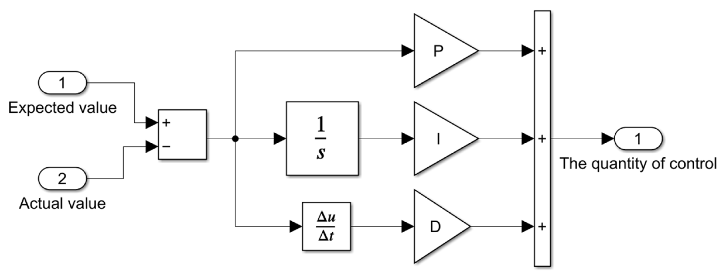
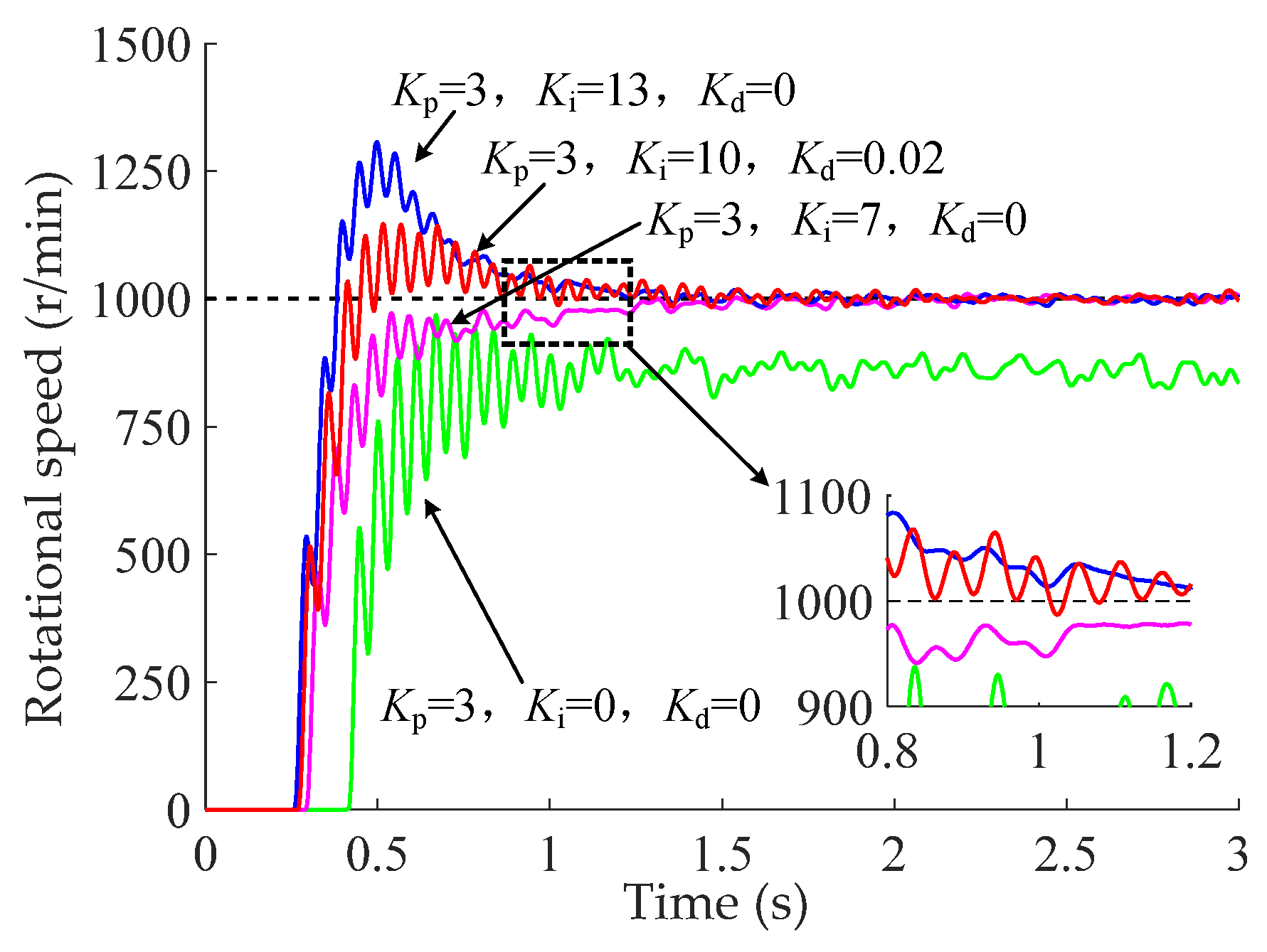
3. Closed-Loop Control Performance Analysis for the DHDS

According to the DHDS simulation model of the EDP in Figure 3, a closed-loop simulation platform for the EDP DHDS is jointly built using AMESim 2020 and Simulink 2020 software, as shown in Figure 5. This closed-loop simulation platform includes the valve control signal module, the load signal module, and the DHDS model. Among them, the reference duty cycle of the composite PWM signal is adjusted by comparing the expected value with the actual value, thereby regulating the input signal of the HSV; the load signal is set using MATLAB 2020, imported into the load signal module LOAD on this simulation platform, and then converted into the load value required by the DHDS of the EDP through formula parameters.

To ensure the rapid response and control accuracy of the rotational speed of the EDP, a DHDS closed-loop control model is established. PID control is adopted to achieve closed-loop speed regulation control and tracking of the hydraulic motor. In this section, the proportional coefficient (K_p), integral coefficient (K_i), and differential coefficient (K_d) of the PID controller are adjusted based on the mechatronic hydraulic-coupling simulation platform. The tracking effect of the target curve is analyzed to obtain the optimal parameter-matching relationship. The expression rule of the PID control algorithm is as follows:

$$u\left(t\right)=K_{\mathrm{p}}e\left(t\right)+K_{\mathrm{i}}{\displaystyle {\int }_0^{t}e\left(t\right)+K_{\mathrm{d}}\frac{\mathrm{d}e\left(t\right)}{\mathrm{d}t}}$$

(39)

Since the DHDS in this study is controlled by a separate HSV for oil intake and return in the control chamber of the HCPRV, and the adjustable duty cycle of the HSV at 100 Hz operating frequency is 0.23~0.83, the input duty cycle signal cannot be negative. To ensure that the curve tracking of closed-loop speed regulation achieved by PID control is not affected by the working state of the HSV, the corresponding logic switch module is designed to enhance the response speed and control the precision of the closed-loop control syste. The PID controller of the DHDS for the EDP was built using Simulink software. The simulation model is shown in Figure 6.

The three control coefficients, K_p, K_i, and K_d, of the PID controller are tuned using the Simulink simulation model illustrated in Figure 6. The target value is set to a step signal of 1000 r/min. The results of the parameter tuning are depicted in Figure 7.

Using only proportional control (K_p = 3) results in fast error reduction but causes large steady-state error and oscillations. To mitigate these issues, an integral term is introduced with K_i initially set at 7, which significantly reduces the steady-state error but extends the response time. Increasing K_i to 13 reduces the response time further, though it leads to excessive overshoot. By adding a derivative term (K_d = 0.02), the overshoot is notably decreased and the response time is slightly improved. The final PID settings are K_p = 3, K_i = 10, and K_d = 0.02, which enhance both the dynamic and static control performance of the digital hydraulic drive system. Based on these PID parameters, trajectory tracking was performed on sine and square wave signals at frequencies of 0.1 Hz and 0.2 Hz, with the results shown in Figure 8 and Figure 9.

It can be deduced from Figure 8 that when the frequency of the square wave signal increases from 0.1 Hz to 0.2 Hz, the adjustment time of the rotational speed increases from 0.84 s to 0.89 s, the rise time increases from 0.25 s to 0.27 s, and the steady-state error improves from 13 r/min to 16 r/min.

As shown in Figure 9, when the frequency of the sinusoidal signal increases from 0.1 Hz to 0.2 Hz, the maximum error rises from 57 to 66 r/min, the average error increases from 32 to 39 r/min, and the standard error grows from 3.69 to 4.5 r/min. Therefore, the signal at 0.1 Hz exhibits slightly better tracking performance than the signal at 0.2 Hz.

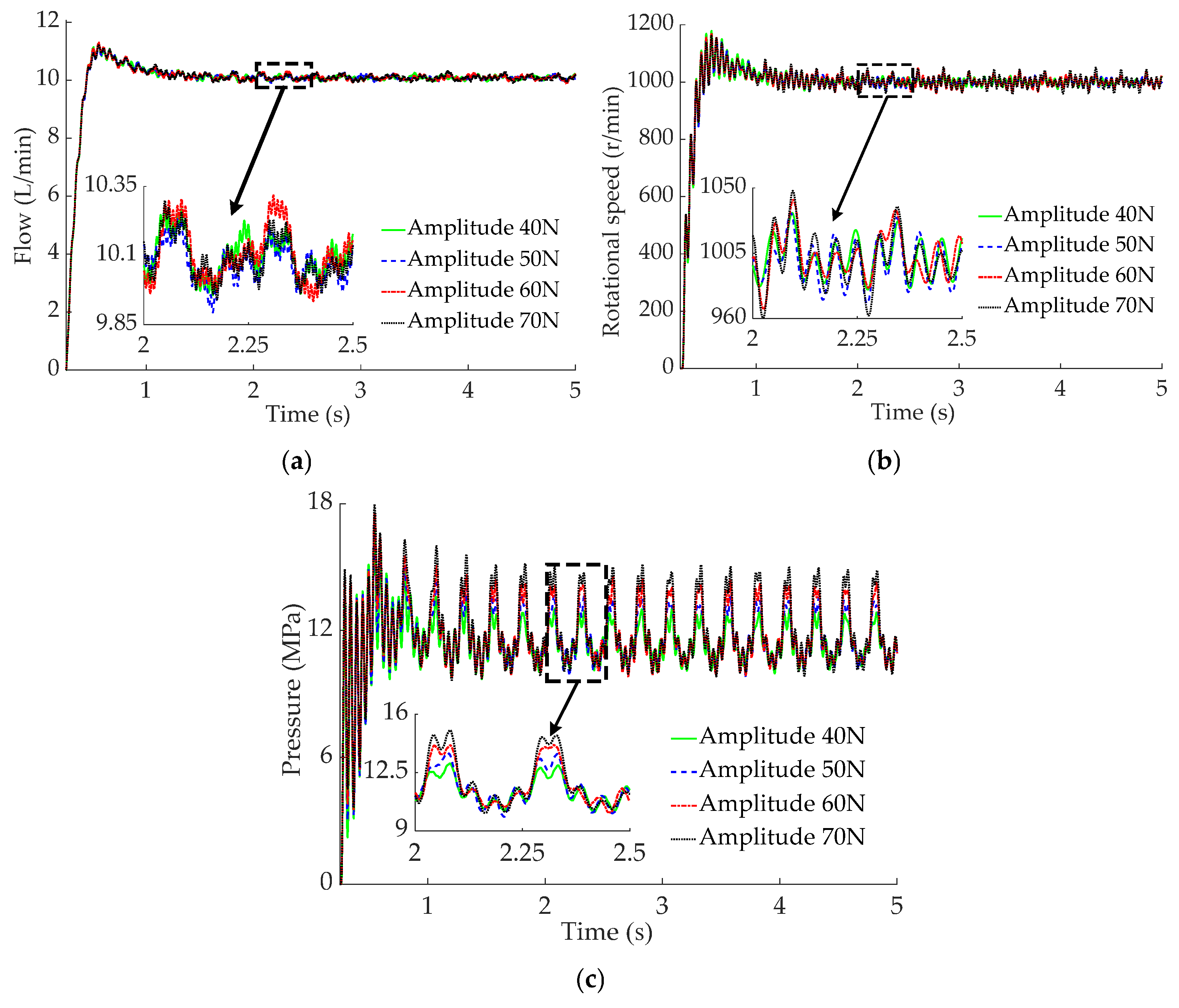
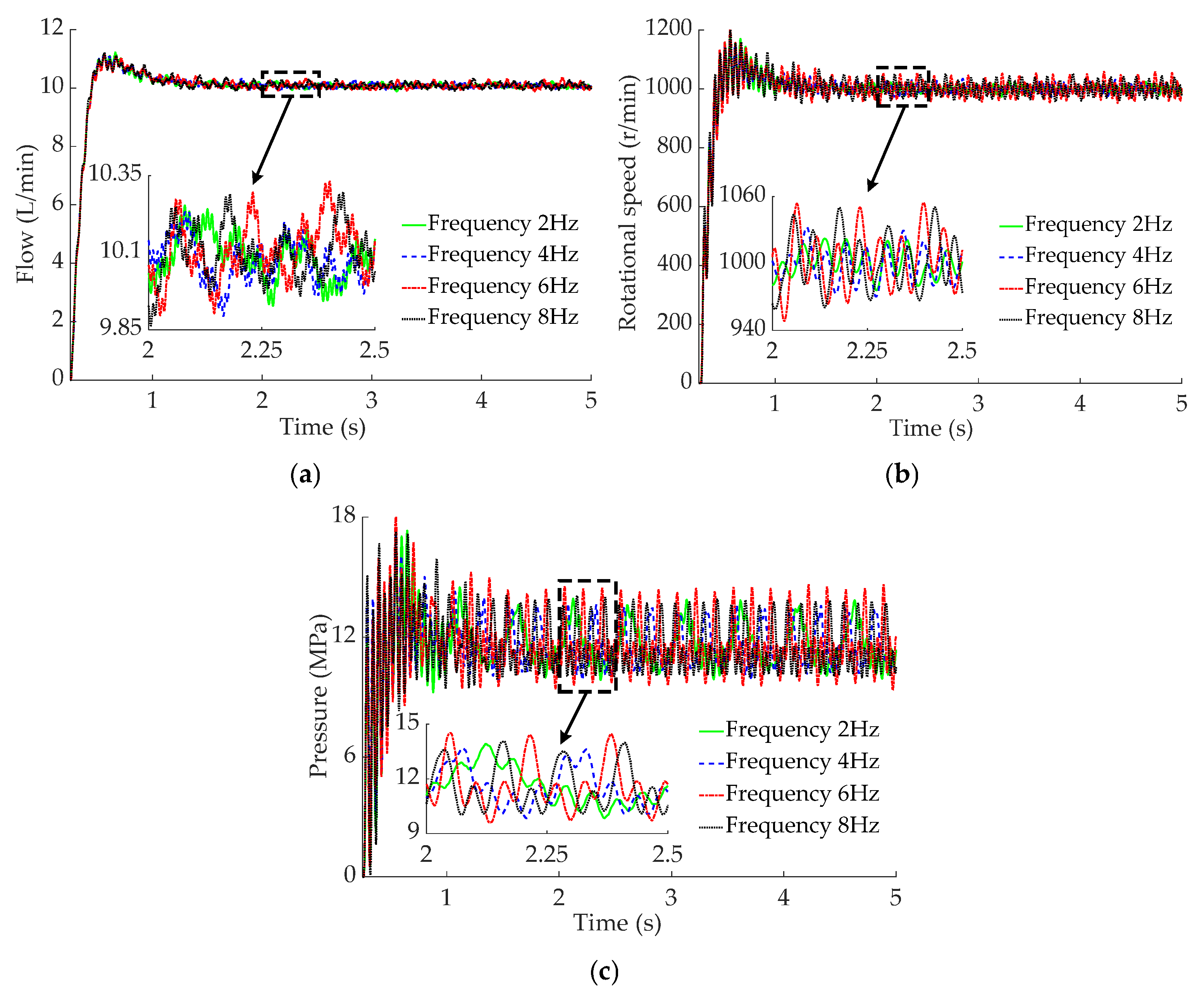
4. Simulation Analysis of the DHDS Under Alternating Loads

To study the action law of alternating loads on the system, alternating loads are classified into three types: different amplitudes, different frequencies, and different waveforms [31]. The amplitudes of the alternating loads were established as 40 N, 50 N, 60 N, and 70 N; the frequencies were from 2 Hz to 8 Hz; and the waveforms were triangular waves and sine waves. The signal distribution of the alternating load is depicted in Figure 10.

Figure 11 summarizes the effects of different alternating-load amplitudes on motor pressure, rotational speed, and output flow. For a 40 N load, during the load increase phase, the motor pressure rises to 13.1 MPa, the rotational speed reaches 1033 r/min, and the output flow peaks at 10.27 L/min; once the load decreases after 0.0625 s, these values drop to 10.16 MPa, 980 r/min, and 9.96 L/min, respectively. As the load amplitude increases, the ranges adjust accordingly: at 50 N, the pressure varies between 10.25 and 13.7 MPa, the rotational speed between 970 and 1032 r/min, and the output flow between 9.9 and 10.22 L/min; at 60 N, the pressure fluctuates from 10.41 to 14.1 MPa, the rotational speed from 966 to 1042 r/min, and the output flow from 9.93 to 10.28 L/min; and at 70 N, the pressure ranges from 9.85 to 15.14 MPa, the rotational speed from 960 to 1048 r/min, and the output flow from 9.92 to 10.3 L/min.

Figure 12 shows that when the alternating-load frequency is 2 Hz, the period of the curve is 0.5 s. At 0.125 s, as the load reaches its peak, the motor pressure peaks at 13.62 MPa, the rotational speed at 1022 r/min, and the output flow at 10.25 L/min. During the subsequent 0.25 s decrease in load, the pressure drops to 10 MPa, the speed to 976 r/min, and the output flow to 9.93 L/min. At 4 Hz, the period is 0.25 s with the rotational speed oscillating between 973 and 1032 r/min; at 6 Hz, the period is 0.17 s with a speed range of 964 to 1050 r/min; and at 8 Hz, the period is 0.125 s with the speed ranging from 959 to 1050 r/min.

Figure 13 shows that with a 50 N alternating load at 4 Hz, all three characteristic curves repeat every 0.25 s, with motor pressure ranging from 9.9 to 13.77 MPa, rotational speed from 973 to 1030 r/min, and output flow from 9.9 to 10.25 L/min. Under a triangular wave load, the rapid changes cause significant internal impacts on the motor, leading to greater buffering in pressure and speed and, consequently, more pronounced output flow oscillations. In contrast, a sine wave load produces gentler fluctuations due to its smaller amplitude variation.

To sum up, when the alternating load increases, the system output characteristics reach the maximum value, and when the load decreases, they drop to the minimum value. During this period, periodic oscillations occur. The increase in the amplitude of the alternating load will cause the amplitude to increase. The increase in the operating frequency will not only increase the amplitude of the system output characteristics but also shorten the variation period of the output characteristics.

5. Experimental Study

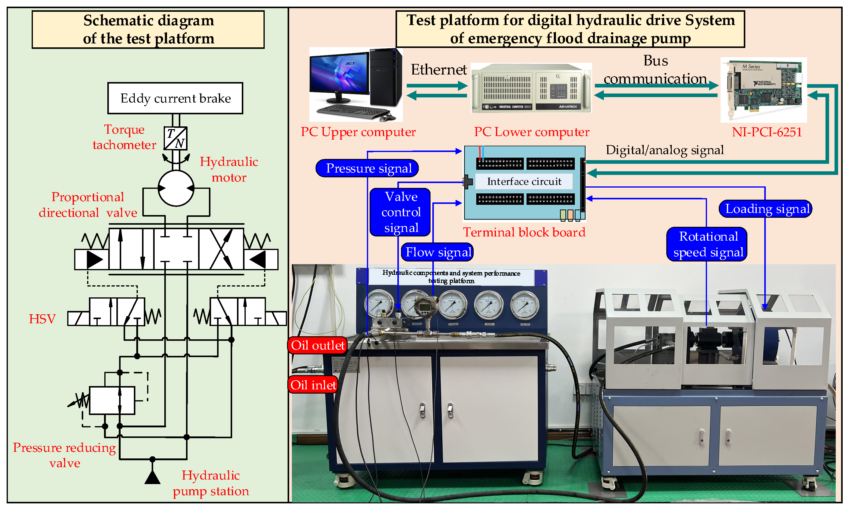
5.1. Test System

To explore the dynamic performance of the DHDS for EDPs and the influence of parameter changes during operation on the dynamic characteristics of the system, a test platform for the EDP DHDS is established. The principle schematic diagram of the experiment system is depicted in Figure 14. The experiment platform is mainly made up of a hydraulic pump station, a hydraulic valve platform, a hydraulic motor brake performance test platform, and a computer control and data acquisition system.

The models and performance parameters of the main components in the test system are as follows:

A CYG1401F-type pressure sensor was selected, with a range of 0~10 MPa, an output signal of 0.1~5 V, an accuracy of 0.5%, and a frequency response of 20 kHz.

A BPMLWGY-type flow sensor was selected, with a measurement range of 3.4 to 20 L/min, an output signal of 4 to 20 mA, and an accuracy of 1%.

A YZJ-type torque and speed sensor was selected. The torque range is −100 to 100 N·m, the speed range is 0 to 6000 r/min, and the accuracy is 0.1%.

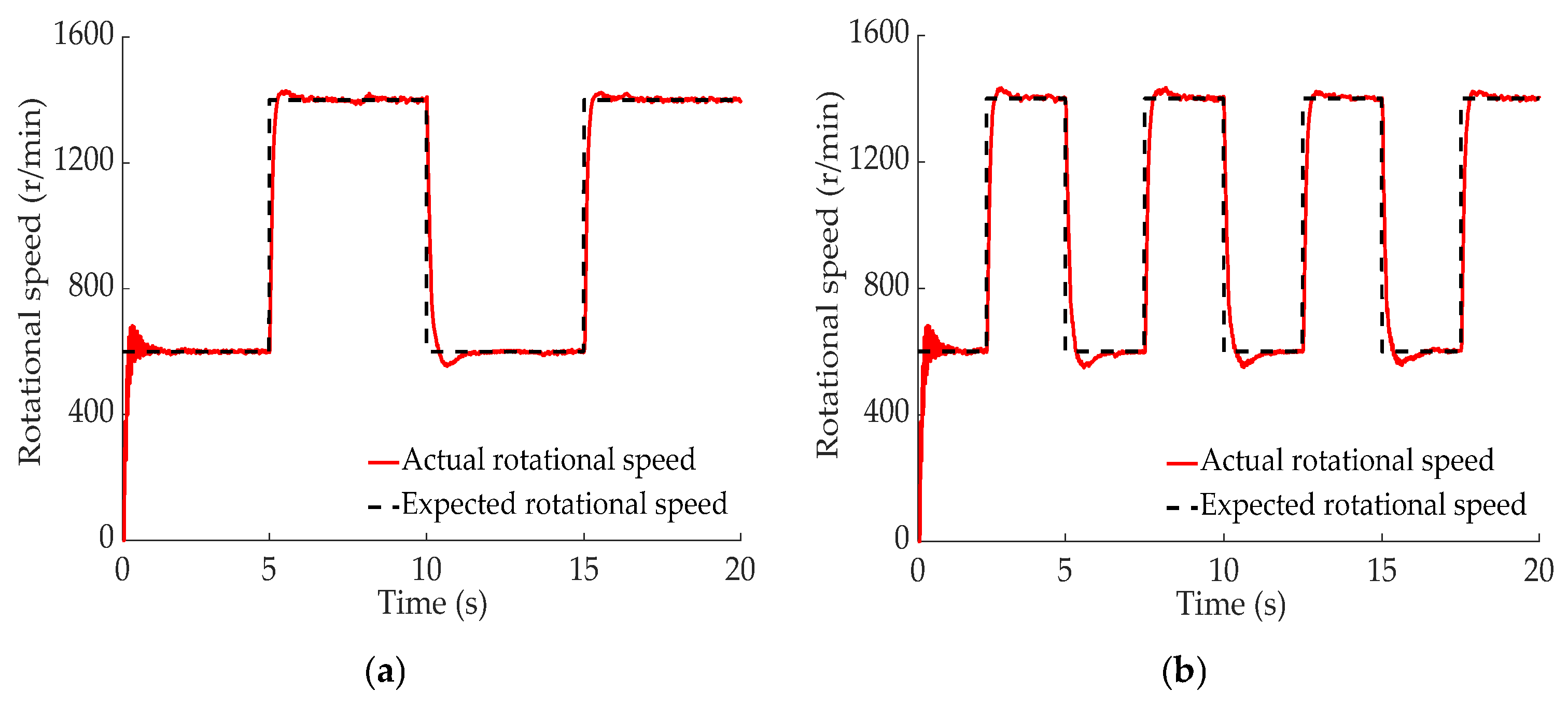
5.2. Closed-Loop Control Performance Test

Due to the differences between the simulation environment and the test environment, situations such as internal leakage of components and losses along the pipeline need to be considered. Therefore, the control parameters determined by the closed-loop simulation study are optimized. Finally, it was determined that the DHDS had better dynamic and static control performance under the following conditions: K_p = 2, K_i = 8, and K_d = 0.02. The expected values of the rotational speed are set to 300, 500, and 700 r/min, respectively, and the test results of the closed-loop control of the system are seen in Figure 15.

It can be deduced from Figure 15 that when the expected rotational speed increases from 300 to 700 r/min, the overshoot of actual rotational speed decreases from 53% to 2.7%, and the stabilization time increases from 3.9 s to 7.1 s. In conclusion, the higher the expected rotational speed is, the smaller the system overshoot will be, but the stabilization time will be relatively longer.

To analyze the response characteristics of the system under closed-loop control, combined with the PID parameters determined by the experiments, tracking tests were conducted, respectively, with square wave signals and sine wave signals of varying amplitudes and frequencies. The tracking results are shown in Figure 16 and Figure 17.

To accurately evaluate the tracking performance of the system for trajectory signals under closed-loop control, in this paper, overshoot, adjustment time, rise time, and steady-state error were adopted as the evaluation indicators of the trajectory-tracking performance of square wave signals, and maximum error, average error, and standard error were adopted as the evaluation indicators of the trajectory-tracking performance of sinusoidal signals. The tracking performance indicators are depicted in

Table 1. Comparison of performance index for square wave and sine wave tracking under a frequency of 0.05Hz and different amplitudes.

Performance Index	Square Wave Signal Amplitude		Performance Index	Sine Wave Signal Amplitude
	200 r/min	400 r/min		200 r/min	400 r/min
Overshoot (%)	31.5	45.7	Maximum error (r/min)	69	87
Adjustment time (s)	2.43	2.65	Average error (r/min)	31	43
Rising time (s)	0.77	0.75	Standard error (r/min)	3.54	4.16
Steady-state error (r/min)	34	23

as follows.

Table 1 shows that a square wave at 200 r/min produces slightly lower overshoot and adjustment time than one at 400 r/min, indicating better response. Likewise, a sinusoidal signal at 100 r/min results in slightly lower maximum, average, and standard errors than one at 200 r/min, reflecting enhanced tracking and stability. Overall, the system performs better with low-amplitude signals, although a slight overshoot or jitter appears as the desired rotational speed decreases.

5.3. Alternating-Load Test

To explore the dynamic response performance of the system under different types of alternating loads, alternating loads were classified into three types: different amplitudes, various frequencies, and different waveforms. It can be seen from the test results of the system under closed-loop control that the stability and subsequent performance are better when the rotational speed of the motor is 700 r/min. Therefore, this section studies the dynamic response characteristics of the DHDS under the action of alternating loads when the rotational speed is 700 r/min. Meanwhile, to prevent pressure shock caused by excessive load and to analyze the dynamic response performance of the system more intuitively, the amplitudes of the alternating loads are set as 5 N·m, 6 N·m, 7 N·m, and 8 N·m, respectively; the frequencies are 0.2 Hz, 0.5 Hz, and 1 Hz, respectively; and the waveforms are triangular waves and sine waves, respectively. The output response performance of the system under different types of alternating loads is shown in Figure 18, Figure 19 and Figure 20.

As shown in Figure 18, when the peak value of the load torque increases from 5 to 8 N·m, the pressure of the motor at the peak point increases from 3.12 MPa to 3.97 MPa. In addition, the output flow of the HCPRV varies slightly with the variation in the amplitude of the alternating load. The fluctuation range of the output flow is 5.61~5.72 L/min. Due to the influence of factors such as flow pulsation and hydraulic pipeline effects, the output flow will have a variation range of 0.11 L/min. The fluctuation range rotational speed enhances with the increase in alternating-load amplitude. The maximum fluctuation range of the rotational speed of the motor is 617~746 r/min.

As is shown in Figure 19, when the frequency of the alternating load rises to 1 Hz, the pressure of the motor gradually increases to 3.52 MPa. When the frequency of the alternating load drops to 0.2 Hz, the pressure of the motor decreases to 2.55 MPa. During the increase in alternating-load frequency, the variation range of the rotational speed is 648~722 r/min. The fluctuation range of the output flow gradually reduced with the increase in frequency, and the maximum fluctuation range is 5.63~5.84 L/min.

In Figure 20, when the alternating load changes suddenly, the pressure in the motor fluctuates between 2.58 and 3.51 MPa. The sine wave curve is smoother than the triangular wave curve. The output flow and rotational speed also undergo periodic changes in line with the load. The flow fluctuates between 5.72 and 5.74 L/min for a sine wave and 5.69 and 5.76 L/min for a triangular wave. The rotational speed remains within 651~721 r/min for different waveforms.

In conclusion, the greater the amplitude of the load torque under an alternating load, the higher the amplitude of the pressure on the motor when it reaches its maximum value and the greater the fluctuation range of the rotational speed. However, the output flow of the HCPRV only changes slightly with the variation in the load torque amplitude. The higher the frequency of the alternating load is, the slower the fluctuation amplitude of the output flow decreases, but the fluctuation range of the pressure and rotational speed of the motor remain basically unchanged. Alternating loads of different waveforms basically do not change the fluctuation range of the pressure and the rotational speed. However, the pressure characteristic curve of the sine wave is smoother and has better continuity than that of the triangular wave, and the fluctuation range of the output flow under the action of sine waves is slightly smaller than that under the action of triangular waves. The research and analysis show that the system can respond quickly to the changes caused by alternating loads under variable working conditions and can recover to a stable state in a short time, verifying that the system has prominent anti-interference ability and output stability.

6. Conclusions

An in-depth analysis and study have been conducted investigating a DHDS for emergency drainage pumps. The EDP DHDS was built, and the influence law of alternating loads on the dynamic response characteristics of the system was explored. The research conclusions are as follows:

(1)

A hydraulic drive system suitable for use in EDPs has been developed, and the working principle of this DHDS has been expounded. The electromechanical hydraulic multi-field coupling dynamic simulation platform of the DHDS for EDPs was further constructed using AMESim and Simulink, and the dynamic response characteristics of the lumped simulation model have been proven.

(2)

Based on the custom functions of the MATLAB software, the parameters of multi-condition loads were set. Variable parameters of amplitude, frequency, and waveform of the alternating loads were also set. The dynamic response characteristics and load action law of the DHDS for EDPs under multi-condition loads was explored. The research and analysis showed that the system can respond quickly to changes in the load under variable working conditions and recover to a stable state in a short time, verifying that the system has good anti-interference ability and output stability.

(3)

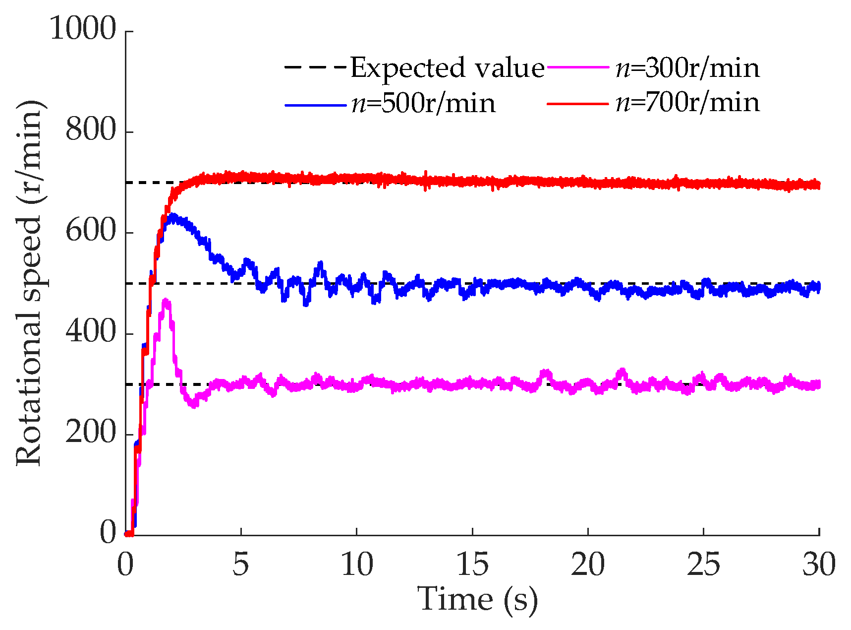
The results of the closed-loop control test showed that when the expected rotational speed is 700 r/min, the overshoot is 2.7%, the stabilization time is 7.1 s, and the stability and followability are good. When tracking square wave signals with amplitudes of 200 r/min and 400 r/min, the overtones are 31.5% and 45.7%, respectively, and the adjustment times are 2.43 s and 2.65 s, respectively. The response characteristics of the square wave signal with an amplitude of 200 r/min are slightly better. When tracking sinusoidal signals with amplitudes of 100 r/min and 200 r/min, the maximum errors are 69 r/min and 87 r/min, respectively, the average errors are 31 r/min and 43 r/min, respectively, and the standard errors are 3.54 r/min and 4.16 r/min, respectively. Thus, the tracking accuracy and stability for the sinusoidal signal with an amplitude of 100 r/min are superior to those for the signal with an amplitude of 200 r/min.

(4)

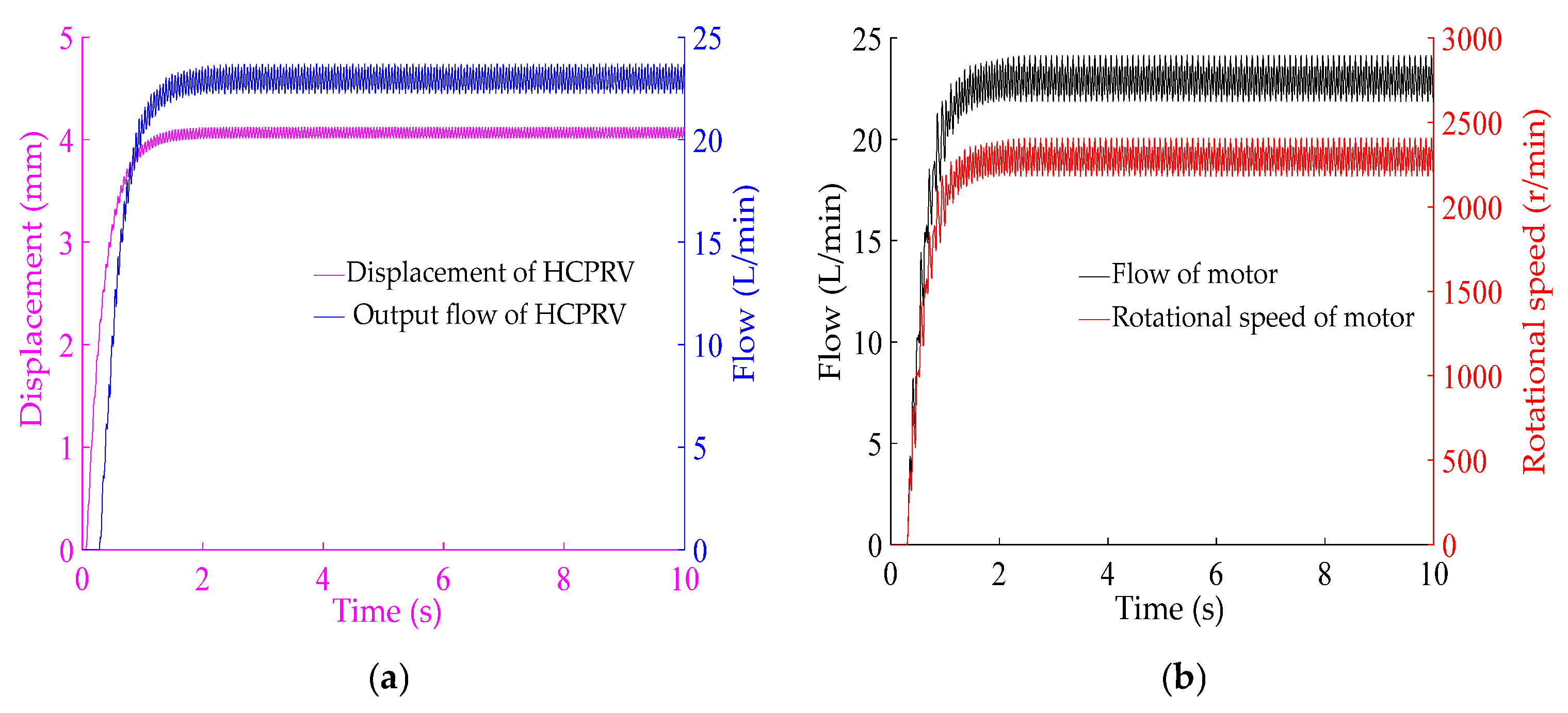
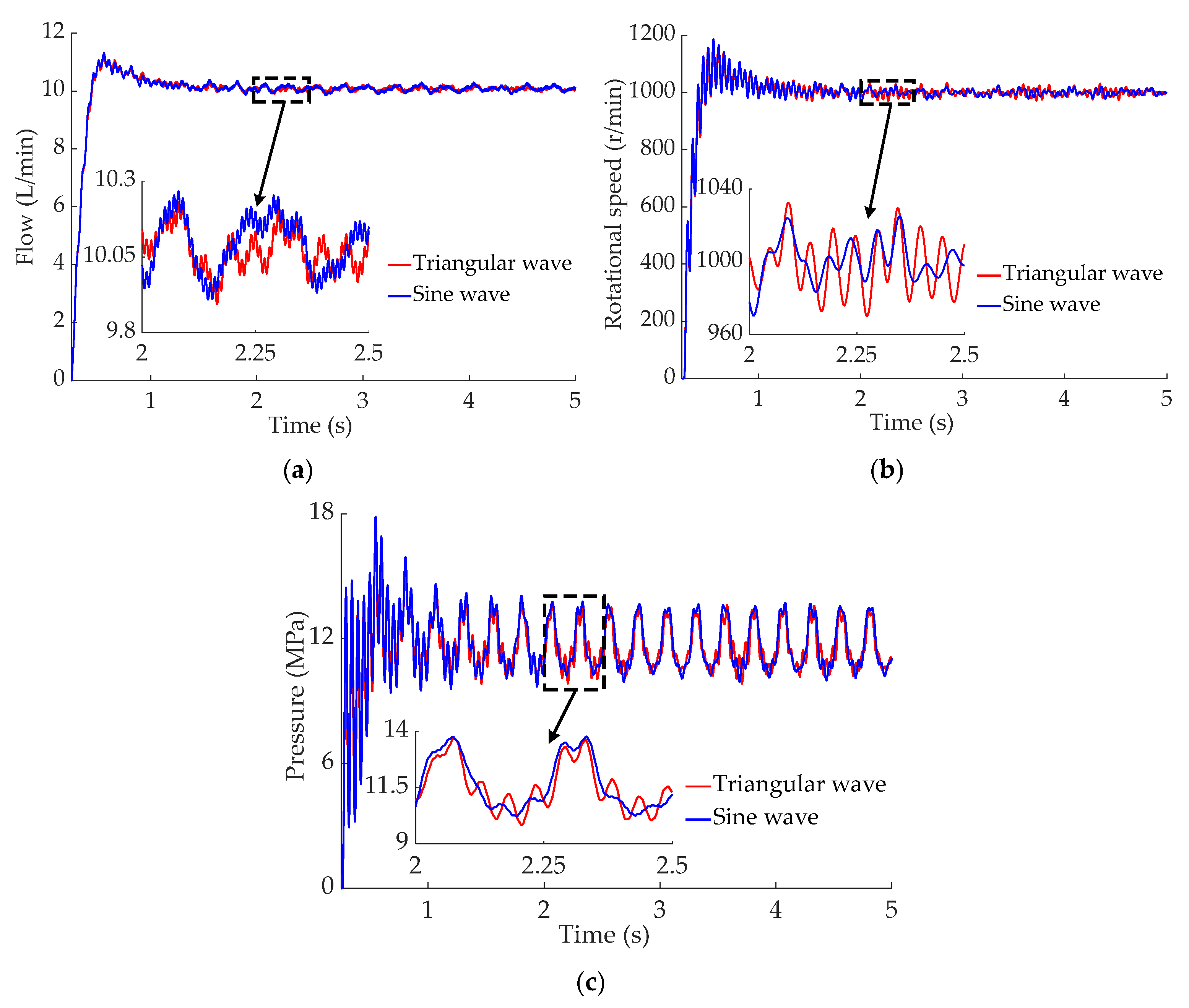
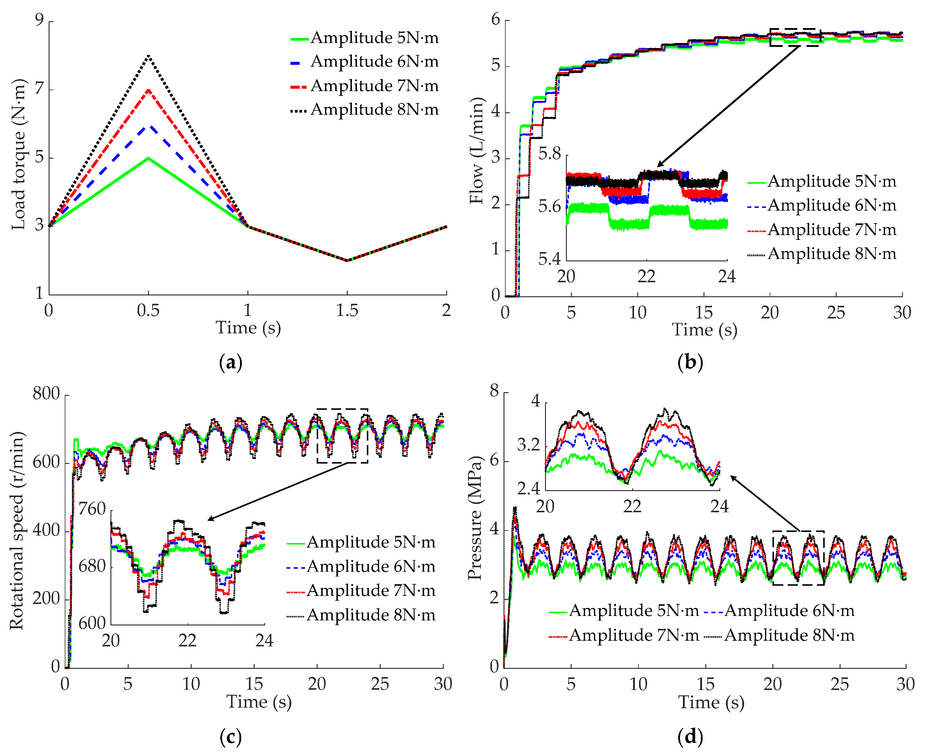
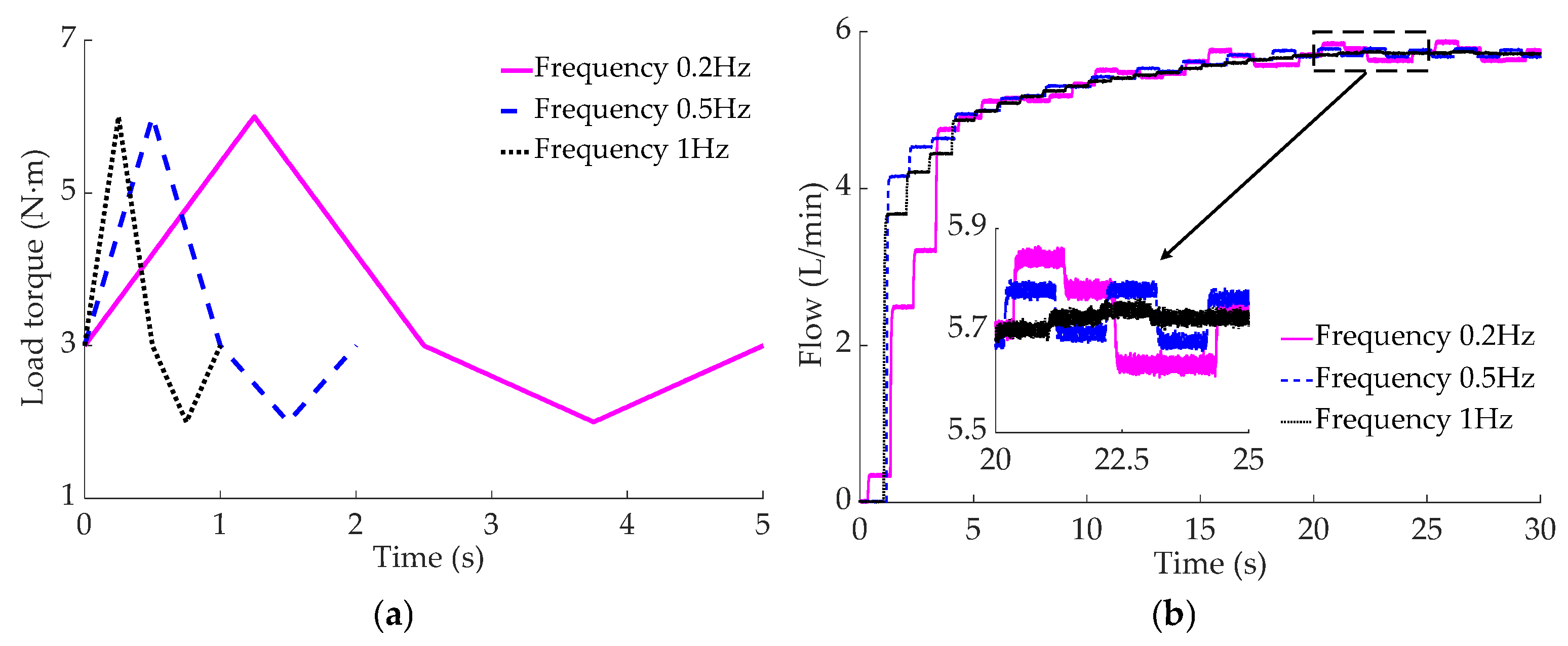
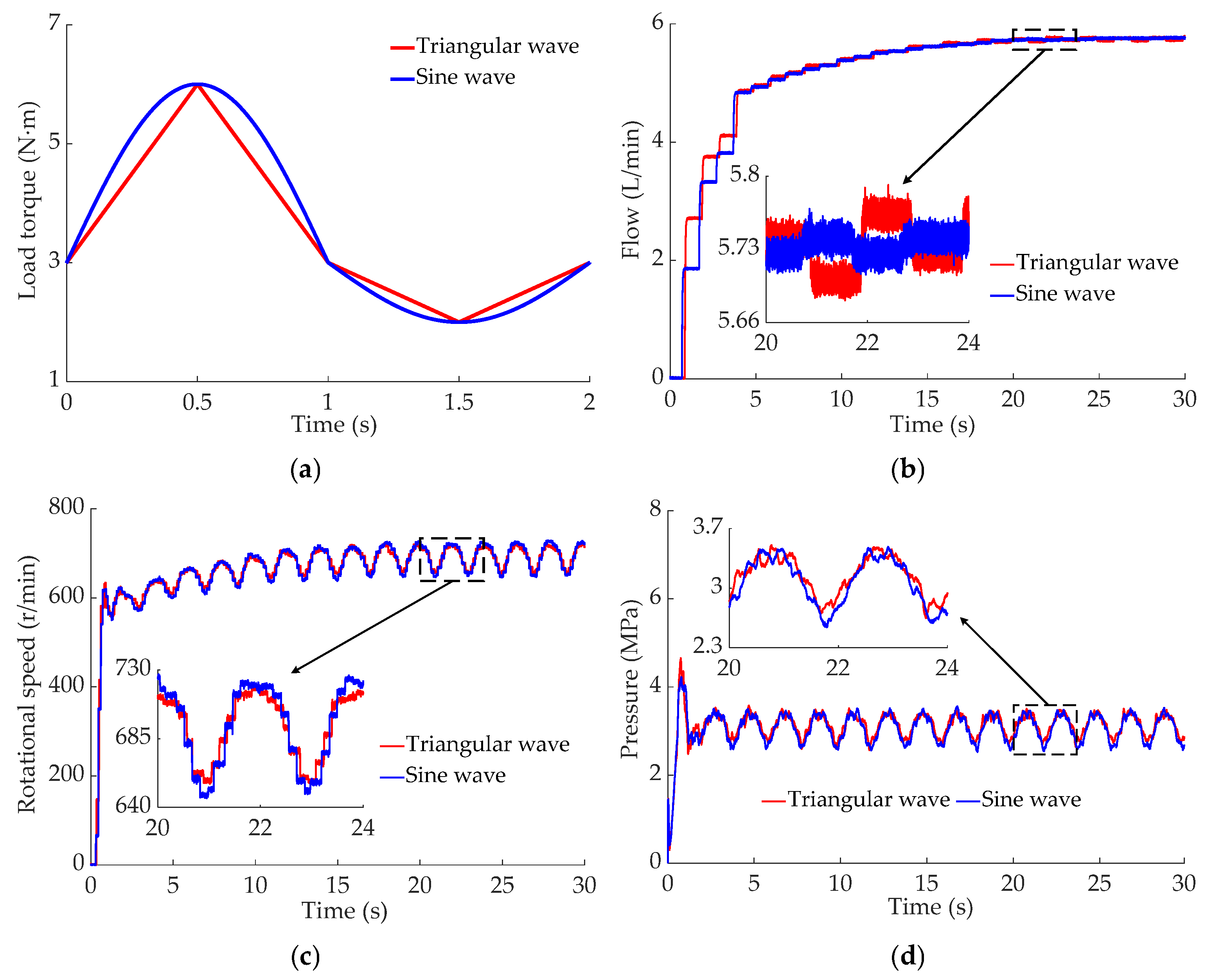
The alternating-load test results indicate that as the load torque enhances from 5 to 8 N·m, the peak pressure of the motor rises from 3.12 to 3.97 MPa, the output flow of the HCPRV fluctuates between 5.61 and 5.72 L/min, and the maximum fluctuation range of the rotational speed of motor extends from 617 to 746 r/min. When the load frequency increases from 0.2 to 1 Hz, the peak value of the pressure of the motor increases from 2.55 to 3.52 MPa, the fluctuation range of the output flow of the HCPRV gradually decreases, and the peak value of the rotational speed of the motor is, at most, 722 r/min. The fluctuation ranges of the pressure and the rotational speed of the motor are basically unaffected by the alternating-load waveforms, which are 2.58~3.51 MPa and 651~721 r/min, respectively. However, the pressure curve of the motor with a sine wave is smoother and has better continuity. The fluctuation range of the output flow of the HCPRV under the influence of the sine wave is slightly smaller. They are 5.72~5.74 L/min and 5.69~5.76 L/min, respectively. The principles derived from the test results are generally in agreement with those from the simulation outcomes.

This study reveals the dynamic response characteristics of the DHDS for EDP under alternating loads, providing a theoretical basis for the revelation of the drive mechanism and stable operation control of EDP, which is powered by digital hydraulics. In the DHDS in this paper, the HSV only adopts PID control. In the future, we will further explore the dynamic response characteristics of EDPs under the control strategies of nonlinear robust control, fuzzy PID, and so on.

References

1. Tian, D.; Si, Q.R.; Liang, K.; Zhang, Y.; Ju, Y.Z.; Yuan, J.P. Study on the Internal Flow Characteristics of High Flowrate Emergency Drainage Series-Parallel Pump. J. Phys. Conf. Ser. 2024, 2854, 012062. [Google Scholar] [CrossRef]
2. Wang, Y.; Wang, X.L.; Liu, H.L.; Xie, L. Optimization and Analysis of Mine Drainage Pump with High Efficiency and Large Flow. J. Low Freq. Noise Vib. Act. 2022, 41, 1091–1107. [Google Scholar] [CrossRef]
3. Rakibuzzaman, M.; Suh, S.H.; Kim, H.H.; Didarul Islam, M.; Zhou, L.; El-Emam, M. Cavitation and Erosion Effects on Hydraulic Performances of a Submersible Drainage Pump. Alexandria Eng. J. 2025, 113, 431–450. [Google Scholar] [CrossRef]
4. Cao, W.D.; Yang, X.Y.; Wang, H.; Leng, X.Y. Numerical Simulation of Gas-Liquid Two-Phase Flow in Emergency Rescue Drainage Pump Based on MUSIG Model. J. Appl. Fluid Mech. 2024, 17, 1730–1745. [Google Scholar]
5. Gong, Y.; Zou, W.H. Optimal Operation of Urban Tidal Drainage Pumping Station Based on Genetic Algorithm Coupled with Head-Water Level Successive Approximation. Front. Energy Res. 2023, 10, 1074529. [Google Scholar] [CrossRef]
6. Huang, X.K.; Wu, X.F.; Tian, Z.Z.; Lin, S.K.; Ji, J.J.; Guo, Y.Y.; Xie, F.W. Fault Diagnosis Study of Mine Drainage Pump Based on MED-WPD and RBFNN. J. Braz. Soc. Mech. Sci. Eng. 2023, 45, 347. [Google Scholar] [CrossRef]
7. Ye, J.; Qin, P.; Xing, Z.R.; Fan, Y.W.; Gao, J.Y.; Deng, Z.S.; Liu, J. Liquid Metal Hydraulic Actuation and Thermal Management Based on Rotating Permanent Magnets Driven Centrifugal Pump. Int. Commun. Heat Mass Transfer 2022, 139, 106472. [Google Scholar] [CrossRef]
8. Kushwaha, P.; Dasgupta, K.; Ghoshal, S.K. A Comparative Analysis of The Pump Controlled, Valve Controlled and Prime Mover Controlled Hydromotor Drive to Attain Constant Speed for Varying Load. ISA Trans. 2022, 120, 305–317. [Google Scholar] [CrossRef]
9. Zhu, Y.; Tang, S.N.; Yuan, S.Q. Multiple-Signal Defect Identification of Hydraulic Pump Using an Adaptive Normalized Model and S Transform. Eng. Appl. Artif. Intell. 2023, 124, 106548. [Google Scholar] [CrossRef]
10. Tang, S.N.; Jiang, Y.X.; Zhou, T.; Zhu, Y.; Lim, K.M. Bayesian Algorithm Optimized Deep Model for Multi-Signal Fault Identification of Hydraulic Pumps. Alexandria Eng. J. 2025, 121, 465–483. [Google Scholar] [CrossRef]
11. Chang, H.; Yang, J.H.; Wang, Z.Q.; Peng, G.J.; Lin, R.Y.; Lou, Y.; Shi, W.D.; Zhou, L. Efficiency Optimization of Energy Storage Centrifugal Pump by Using Energy Balance Equation and Non-dominated Sorting Genetic Algorithms-II. J. Energy Storage 2025, 114, 115817. [Google Scholar] [CrossRef]
12. Tang, S.N.; Jiang, Y.X.; Su, H.; Zhu, Y. A Fault Identification Method of Hydraulic Pump Fusing Long Short-Term Memory and Synchronous Compression Wavelet Transform. Appl. Acoust. 2025, 232, 110553. [Google Scholar] [CrossRef]
13. Wang, Z.; Chen, Y.J.; Rakibuzzaman, M.; Agarwal, R.; Zhou, L. Numerical and Experimental Investigations of a Double-Suction Pump with a Middle Spacer and a Staggered Impeller. Irrig. Drain. 2025, 74, 944–956. [Google Scholar] [CrossRef]
14. Zhao, Z.J.; Jiang, L.; Bai, L.; Pan, B.; Zhou, L. Numerical Simulation and Entropy Production Analysis of Centrifugal Pump with Various Viscosity. Comput. Model. Eng. Sci. 2024, 141, 1730–1745. [Google Scholar] [CrossRef]
15. Pang, Y.Y.; Tang, P.; Li, H.; Marinello, F.; Chen, C. Optimization of Sprinkler Irrigation Scheduling Scenarios for Reducing Irrigation Energy Consumption. Irrig. Drain. 2024, 73, 1329–1343. [Google Scholar] [CrossRef]
16. Wang, W.T.; Chao, Q.; Shi, J.J.; Liu, C.L. Condition Monitoring of Axial Piston Pumps Based on Machine Learning-Driven Real-Time CFD Simulation. Eng. Appl. Comput. Fluid Mech. 2025, 19, 2474676. [Google Scholar] [CrossRef]
17. Sciatti, F.; Tamburrano, P.; Distaso, E.; Amirante, R. Digital Hydraulic Technology: Applications, Challenges, and Future Direction. J. Phys. Conf. Ser. 2023, 2648, 012053. [Google Scholar] [CrossRef]
18. Gao, Q.; Wang, J.; Zhu, Y.; Wang, J.; Wang, J.C. Research Status and Prospects of Control Strategies for High Speed On/Off Valves. Processes 2023, 11, 160. [Google Scholar] [CrossRef]
19. Yang, S.; Yao, J.; Wang, P.; Zhang, P.Y.; Wei, T.F.; Li, D.M. A Novel Dual-Magnetic Circuit Actuated Fast-Switching Valve with Multi-Stage Excitation Control Algorithm. Measurement 2024, 230, 114483. [Google Scholar] [CrossRef]
20. Xu, E.G.; Zhong, Q.; He, X.J.; Mao, Y.X.; Huang, Y.; Yang, H.Y. A Novel Current-Based Identification Method for Dynamic Performance of High-Speed On/Off Valve. Measurement 2024, 232, 114719. [Google Scholar] [CrossRef]
21. Gao, Q.; Liu, H.Y.; Lan, B.; Zhu, Y. A Model-based Sliding Mode Control with Intelligent Distribution for a Proportional Valve Driven by Digital Valve Arrays. ISA Trans. 2024, 151, 312–323. [Google Scholar] [CrossRef]
22. Huang, S.; Zhou, H. Optimizing Multi-Coil Integrated High-Speed On/Off Valves for Enhanced Dynamic Performance with Voltage Control Strategies. Appl. Comput. Electrom. 2024, 39, 1019–1034. [Google Scholar] [CrossRef]
23. Kogler, H. High Dynamic Digital Control for a Hydraulic Cylinder Drive. Proc. Inst. Mech. Eng. Part I J. Syst. Control Eng. 2022, 236, 382–394. [Google Scholar] [CrossRef]
24. Gao, Q. Nonlinear Adaptive Control with Asymmetric Pressure Difference Compensation of a Hydraulic Pressure Servo System Using Two High Speed On/Off Valves. Machines. 2022, 10, 66. [Google Scholar] [CrossRef]
25. Yang, X.; Wu, D.F.; Wang, C.L.; Gao, C.Q.; Gao, H.; Liu, Y.S. Adaptive Fuzzy PID Control of High-Speed On-Off Valve for Position Control System Used in Water Hydraulic Manipulators. Fusion Eng. Des. 2024, 203, 114437. [Google Scholar] [CrossRef]
26. Li, Q.Z.; Hao, P.; Wang, J.; Deng, H. Pulse-Width-Modulation-Based Ttime-Delay Compensation Control for High-Speed On/Off Valves. Electronics. 2023, 12, 3627. [Google Scholar] [CrossRef]
27. Zhong, Q.; Mao, Y.X.; Xu, E.G.; Wang, X.L.; Li, Y.B.; Yang, H.Y. Fast Dynamics and Low Power Losses of High-Speed Solenoid Valve Based on Optimized Pre-Excitation Control Algorithm. Therm. Sci. Eng. Prog. 2024, 47, 102363. [Google Scholar] [CrossRef]
28. Zhong, Q.; Wang, J.X.; Xu, E.G.; Yu, C.; Li, Y.B. Multi-Objective Optimization of a High Speed On/Off Valve for Dynamic Performance Improvement and Volume Minimization. Chin. J. Aeronaut. 2024, 37, 435–444. [Google Scholar] [CrossRef]
29. Stosiak, M.; Karpenko, M. The Influence of the Hydropneumatic Accumulator on the Dynamic and Noise of the Hydrostatic Drive Operation. Eksploat. Niezawodn. 2024, 26, 2. [Google Scholar] [CrossRef]
30. Stosiak, M.; Karpenko, M.; Ivannikova, V.; Maskeliunaite, L. The Impact of Mechanical Vibrations on Pressure Pulsation, Considering the Nonlinearity of the Hydraulic Valve. J. Low Freq. Noise Vib. Act. Control 2024, 44, 706–719. [Google Scholar] [CrossRef]
31. Guo, D.D.; Wang, M.; Jiang, N.; Zeng, Y.Y.; Cao, H.Q.; Wang, D.Y.; Lu, J.; Wu, D.Y. Operation Characteristics of Soil Blasting Vibration Test Device under Vibration Load. Rev. Sci. Instrum. 2023, 94, 045007. [Google Scholar] [CrossRef]
Figure 1. Schematic diagram of the DHDS for EDPs. 1—power unit; 2—hydraulic valve control unit; 3—execution unit.
Machines 13 00636 g001
Figure 2. Schematic diagram of power unit. 1—oil suction filter; 2—pump; 3—direct-acting relief valve; 4—pilot-operated proportional relief valve; 5—electromagnetic directional control valve; 6—cooler; 7—accumulator.
Machines 13 00636 g002
Figure 3. Simulation model of the DHDS for EDPs.
Machines 13 00636 g003
Figure 4. Simulation results: (a) displacement and output flow of the HCPRV; (b) flow and rotational speed of the motor.
Machines 13 00636 g004
Figure 5. Closed-loop simulation platform of a DHDS for EDPs.
Machines 13 00636 g005
Figure 6. Simulation model of PID controller.
Machines 13 00636 g006
Figure 7. Comparison of the simulation results for PID parameter tuning.
Machines 13 00636 g007
Figure 8. Simulation results of a closed-loop control system tracking different frequencies of square wave signal: (a) 0.1 Hz; (b) 0.2 Hz.
Machines 13 00636 g008
Figure 9. Simulation results of the closed-loop control system tracking different frequencies of sine signal: (a) 0.1 Hz; (b) 0.2 Hz.
Machines 13 00636 g009
Figure 10. Signal of alternate loads: (a) amplitudes; (b) frequencies; (c) waveforms.
Machines 13 00636 g010
Figure 11. System response characteristics with a frequency of 4 Hz and different amplitudes: (a) flow; (b) rotational speed; (c) pressure.
Machines 13 00636 g011
Figure 12. System response characteristics with a amplitude of 50 N and different frequencies: (a) flow; (b) rotational speed; (c) pressure.
Machines 13 00636 g012
Figure 13. System response characteristics with an amplitude of 50 N, a frequency of 4 Hz, and different waveforms: (a) flow; (b) rotational speed; (c) pressure.
Machines 13 00636 g013
Figure 14. Schematic diagram of the DHDS for EDPs.
Machines 13 00636 g014
Figure 15. Rotational speed characteristic of a hydraulic motor under closed-loop control.
Machines 13 00636 g015
Figure 16. Experimental results of closed-loop control system tracking with 0.05 Hz square wave signals: (a) amplitude 200 r/min; (b) amplitude 400 r/min.
Machines 13 00636 g016
Figure 17. Experimental results of closed-loop control system tracking with 0.1 Hz sine wave signals: (a) amplitude 100 r/min; (b) amplitude 200 r/min.
Machines 13 00636 g017
Figure 18. System response characteristics with a frequency of 4 Hz and different amplitudes: (a) alternating loads; (b) flow; (c) rotational speed; (d) pressure.
Machines 13 00636 g018
Figure 19. System response characteristics with a load torque of 6 N·m and different frequencies: (a) alternating loads; (b) flow; (c) rotational speed; (d) pressure.
Machines 13 00636 g019aMachines 13 00636 g019b
Figure 20. System response characteristics with load torque of 6 N·m, a frequency of 4 Hz, and different waveforms: (a) alternating loads; (b) flow; (c) rotational speed; (d) pressure.
Machines 13 00636 g020