Development of an Advanced Wear Simulation Model for a Racing Slick Tire Under Dynamic Acceleration Loading

Abstract

This study investigates the development of a tire wear model using finite element techniques. Experimental testing was conducted using the Hoosier R25B slick tire mounted onto a Mustang Dynamometer (MD-AWD-500) in the Automotive Center of Excellence, Oshawa, Ontario, Canada. A general acceleration/deceleration procedure was performed until the battery was completely exhausted. A high-fidelity finite element tire model using Virtual Performance Solution by ESI Group, a part of Keysight Technologies, was developed, incorporating highly detailed material testing and constitutive modeling to simulate the tire’s complex mechanical behavior. In conjunction with a finite element model, Archard’s wear theory is implemented algorithmically to determine the wear and volume loss rate of the tire during its acceleration and deceleration procedures. A novel application using a modified wear theory incorporates the temperature dependence of tread hardness to measure tire wear. Experimental tests show that the tire loses 3.10 g of mass within 45 min of testing. The results from the developed finite element model for tire wear suggest a high correlation to experimental values. This study demonstrates the simulated model’s capability to predict wear patterns, ability to quantify tire degradation under dynamic loading conditions and provides valuable insights for optimizing performance and wear estimation.

1. Introduction

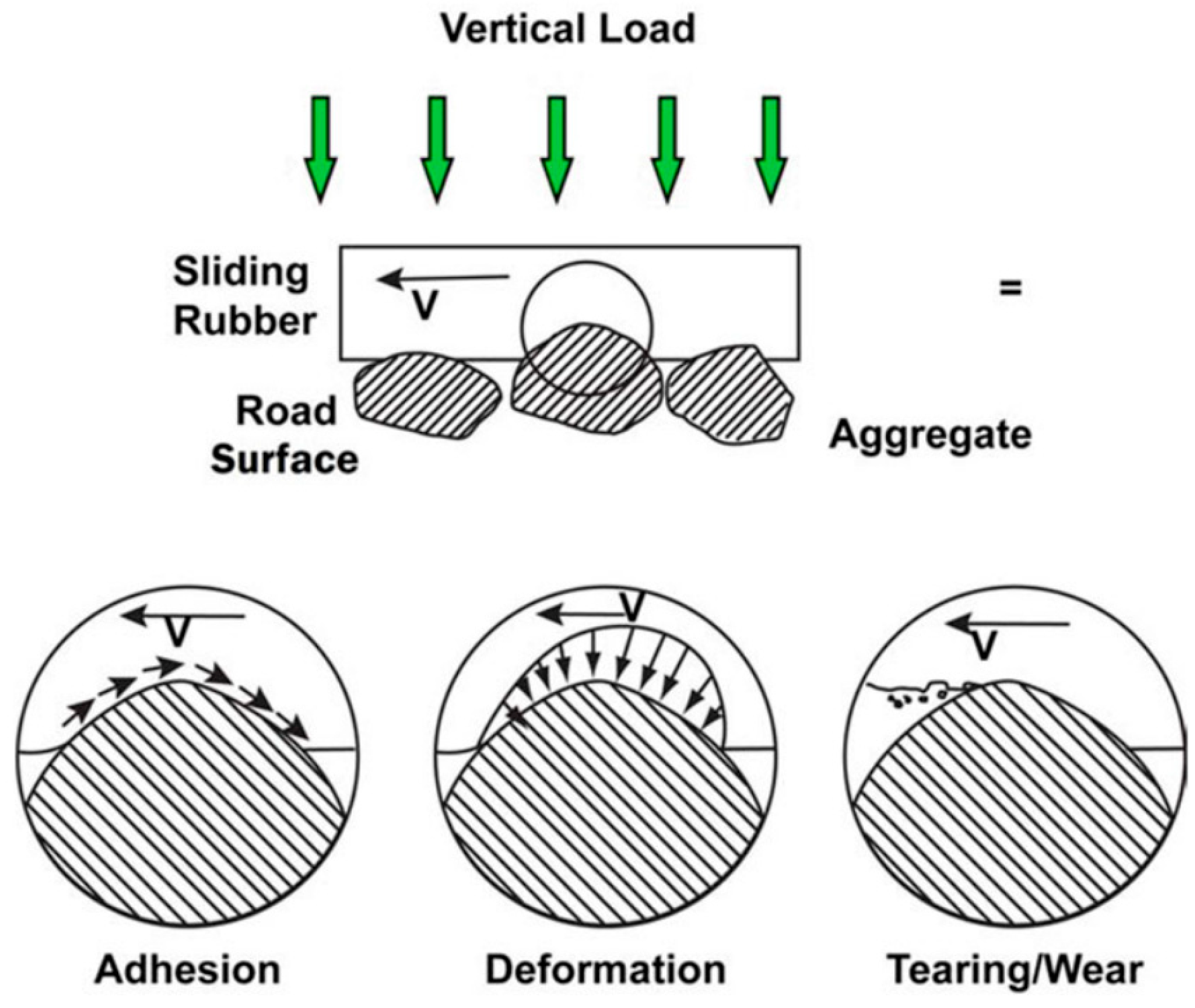
The tire rubber wear phenomenon is defined as the result of energy dissipation into friction. Energy dissipation is largely characterized by tire adhesion and hysteresis. In general, there are three components to rubber friction: adhesion, deformation, and abrasion, as in Figure 1 [1]. Adhesion is present when two sliding surfaces slide on one another with some pressure. Hysteresis, on the other hand, is a material characteristic that defines the response of a deformed subject returning to its normal state from compression or expansion [2,3]. For viscoelastic tire materials, the hysteresis wear occurs from the material being penetrated by the asperities of the road onto the tire, whilst developing high and low deformation areas. When the tire slides at any point over a surface in this fashion, the rubber creates a pressure hysteresis in the tire. This is generally a mild type of wear; however, depending on the material and material-dependent properties like temperature, the process can be exponential.

Experimental-based methodologies to estimate tire wear involve quantitative measuring tools such as sensor data. The data is then used to relate to tire-road frictional data to estimate a wear model. Khaleghian et al. [4] describe the experimental approach in three steps: obtaining wear-related parameters, correlating the data through wear-related formulations, and estimating the tire wear.

In 2002, Grosch [5] developed an abrasion testing machine for empirical tire wear simulations. Grosch’s experimental procedure uses a sample piece of a tire attached to a mount that rolls over an abrasive disc. This machine is titled the Grosch machine, or the Laboratory Abrasion and Skid Tester (LAT) 100. In this test, the lateral force at a given slip angle is observed.

Simulated tire wear approaches are the analysis of tire wear using theoretical, mathematical, or computer-aided simulated models. DaSilva et al. [6] used a similar approach of formulating wear with abrasion, like in Grosch’s work, but theoretically in the form of the bicycle model. This tire wear model was an estimation using only steady-state cornering maneuvers and a 2-degree-of-freedom bicycle model. In this model, any lateral load transfer was negligible, and no tire suspension characteristics were considered. Additionally, the model is only valid for low lateral accelerations.

In 2011, Chang et al. [7] developed a Finite Element Analysis (FEA) tire wear model with a programmed subroutine using the Archard wear model. This model was a simple sliding abrasion relationship between two surfaces. This study analyzed the wear using Archard’s wear model under straight free rolling and driven conditions and estimated tire wear as a function of mass and depth. In 2014, Zang et al. [8] combined FEA tire wear testing and neural network tools to estimate tire wear. In this study, an FEA tire model using the Neo-Hookean tread material equipped with constant shear and unconditional stability is used in several varying simulations. This analysis looks at a particular material type, and the neural network is trained for input variables of inflation pressure, speed, load, and different vibrational frequencies of the tire. In 2017, Wu et al. [9] researched a semi-empirical model of wear using FEA and the LAT100 wear test machine. This model uses the LAT100 with a rubber specimen, but simulates a rolling tire on a wheel within FEA. This study showed that the wear rate is exponential to the friction energy rate. In similar studies, it was also noticed in tire wear simulation that footprint frictional energy dissipation is the main cause of tire wear [10,11]. In 2013, Dumitriu et al. [12] worked on an FEA friction model using Coulomb’s law, which yielded results that agreed with experimental data. Konde et al. [13] did similar research for an aircraft tire, also using Coulomb’s law, which yielded agreeable results with experiments. In 2015, Alroqi et al. [14] developed a tire model that uses a mass-spring-damper system to measure vertical loads for a tire wear model. This model also implemented Archard’s wear theory depending on tire normal load, hardness and slip ratio. This model uses a generic load model alongside a simplified wear model for a tire that is mostly locked and sliding on asphalt. In 2021, Hartung et al. [15] developed a tire wear model on the block level. This study looked at the tire wear of a portioned block of tire rubber pressed and sliding over a track. This model also used Archard’s wear theory to simulate the tire block wear using Coulomb’s law. In 2022, Li et al. [16] developed a finite element tire model capable of simulating tire wear using Archard’s wear theory. This tire was limited in validation as it was only statically tested against experimental results. The wear simulation implementation also lacks temperature and hardness modeling using constant values from varying literature. In 2023, Zhang et al. [17] did similar research, developing a tire wear model using finite element models, studying the impact of cornering. However, similar limitations were seen with temperature, material hardness, and overall tire validation against experimental results.

This study aims to advance the work in tire wear modeling by developing a wear model process using the finite element method and MATLAB R2025a. The model incorporates a high-fidelity tire model that was comprehensively validated against experimental results. This should yield a highly accurate friction dissipation energy rate at its contact patch within the simulation. Following this, a modified Archard’s wear theory is used, incorporating a temperature-dependent hardness model and a velocity-dependent friction model. By utilizing in-house tire modeling, material testing, and custom tire wear testing, an agreeable wear test method is proposed. This research provides insight into the clear gaps in the current body of literature for tire wear simulation. The novel wear model presented in this research uses a highly validated tire model in both static and dynamic domains. Also, the tire wear model incorporates a tread hardness-temperature correlation for dynamic tire maneuvering. The model simulates the tread wear for a dynamic rolling tire through acceleration and deceleration procedures and is validated against controlled experimental tests. The insights provided from this body of work will contribute to the understanding of tire wear mechanics and support the development of tire wear measurement methods.

2. Experimental Testing

This section outlines the experimental setup for acquiring physical data on the R25B tire wear model. The dynamometer, vehicle setup, tire setup, specifications, and data acquisition are comprehensively presented.

2.1. Dynamometer and Vehicle Setup

The vehicle used in this study is the Formula Society of Automotive Engineers (FSAE) F22 Ontario Tech University (OTU) race car. The F22 is an all-electric race car that was custom-designed and built at OTU in Oshawa, Canada for FSAE competition. This vehicle is equipped with a 400 V battery pack, a 5.76 kWh capacity, and a max output power of 80 kW. The battery powers the EMRAX 208 High Voltage (HV) motor that has a peak torque rating of 150 Nm and a continuous torque rating of 90 Nm. This vehicle was chosen for this wear study as all information and data sets regarding the F22 are well documented, including some tire data. Furthermore, being an engineering development vehicle, it was additionally equipped with data acquisition tools to measure all aspects of vehicle performance. Additionally, the electric motor power delivery of the vehicle made it very capable of controlled and consistent tire tests.

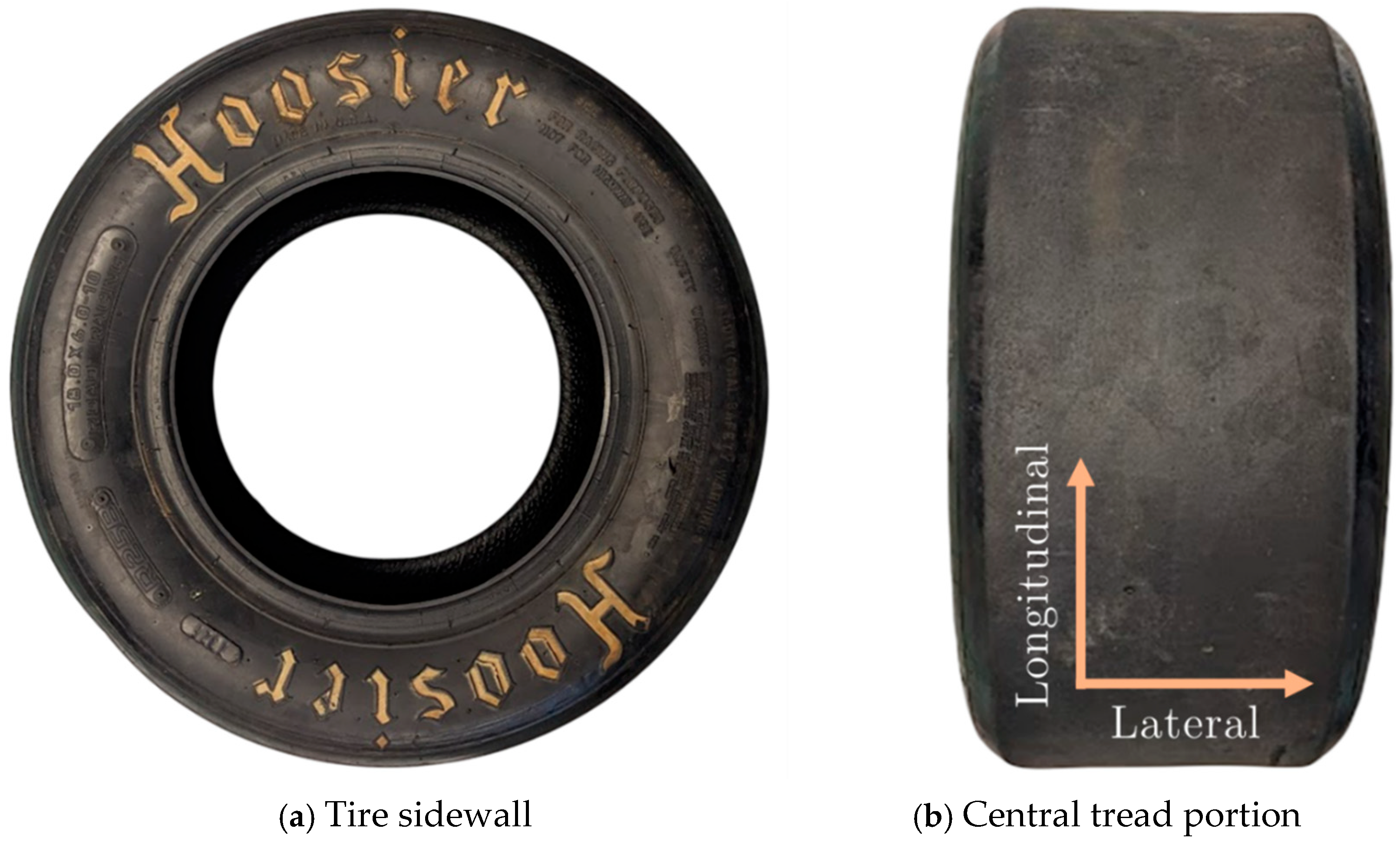
The 18.0X6.0-10 Hoosier R25B tires were set on 10-inch rims, and their tire data was available through the Calspan Corporation and FSAE Tire Test Consortium (TTC). Since the test was completed on a full vehicle setup, the acceleration data and tire wear data would prove useful for analysis on the vehicle’s actual dynamics for performance and future work.

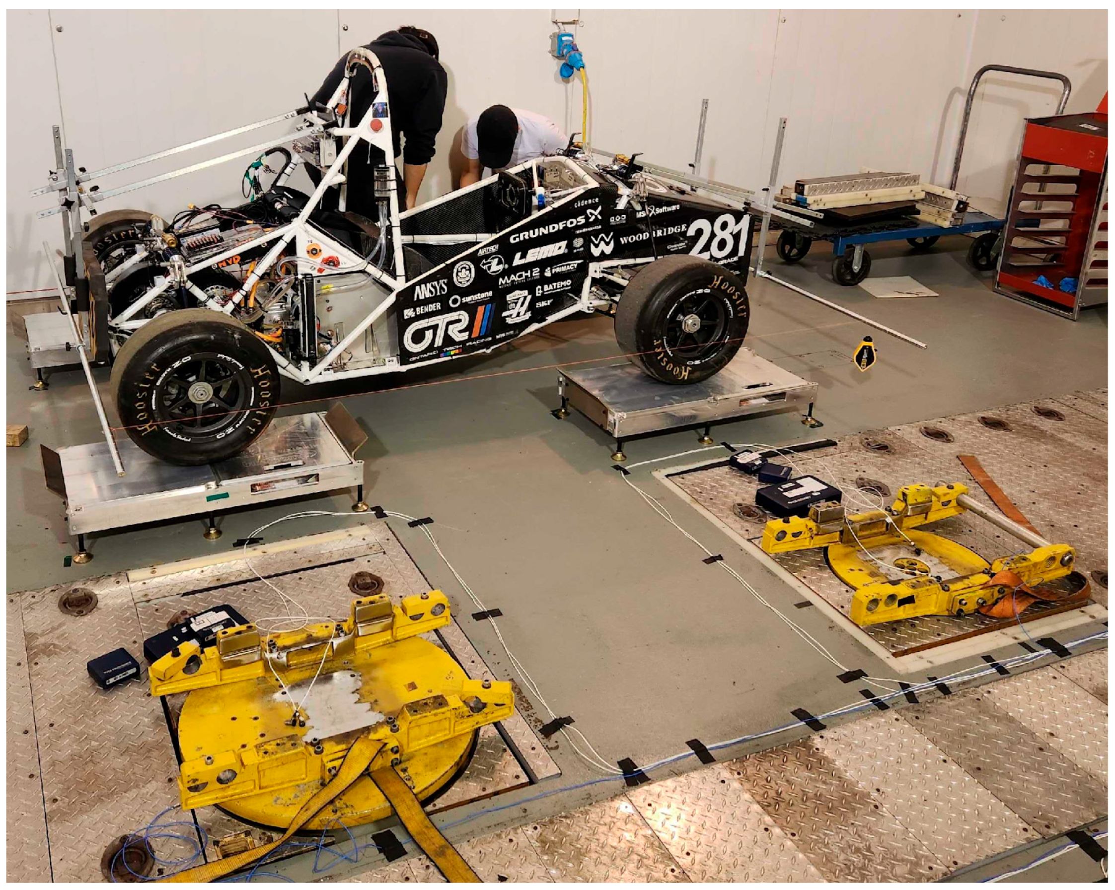
Before wear testing, the vehicle needed to be mechanically conditioned and set up for the required experiments. The vehicle and wheel setup were calibrated for weight and alignment as seen in Figure 2. This was required for high-accuracy measurements for pretest measurements, post-test measurements, and the creation of virtual sensors. The alignment process consisted of using a rigid fixture referenced from the chassis of the vehicle to 4 datum points outside the perimeter of the wheels and centered at the wheel center. Using a string to link each of the datums on each side of the vehicle, a measurement can be taken at the fore and aft points on each of the wheel rims about its center. Using these measurements, the toe angle of each wheel could be adjusted and set. The corner weights were set using precision scales on each wheel, placed on pads leveled to the floor. By adjusting the pre-load on the springs and the push rods, the ride height and corner weights were set to the desired target for testing.

Once this was completed, the vehicle was ready to be strapped onto the dynamometer. The dynamometer used was a Mustang MD-AWD-500 series chassis dynamometer. This dynamometer is used for a vast variety of vehicle testing, including tire testing. The system is capable of handling AWD drive systems, but for this test, it was used in single axle mode. The rear wheels were placed onto the single-axle dynamometer steel drum. The steel drum was manufactured with a knurled pattern to maintain grip. The drum was also painted yellow, whose importance will be discussed later in the Section 4.

The Mustang MD-AWD-500 series chassis dyno uses an internal drive system. It can achieve a max horsepower (hp) of 3000 hp and a max absorption of 1800 hp. The MD-AWD-500 is equipped with an air-cooled eddy current power absorber (MDK-250) loading device and uses a closed-loop strain gauge dynamic load cell for torque measurements. It is rated for 2000 lbs. of inertia in the 2-wheel drive mode and 3625 lbs. in the all-wheel drive mode. The knurled steel drum is precision-machined and dynamically balanced. The dimensions are 370.675 mm in diameter, with a face length of 939 mm, inner track width of 609 mm, and outer track width of 2489.20 mm.

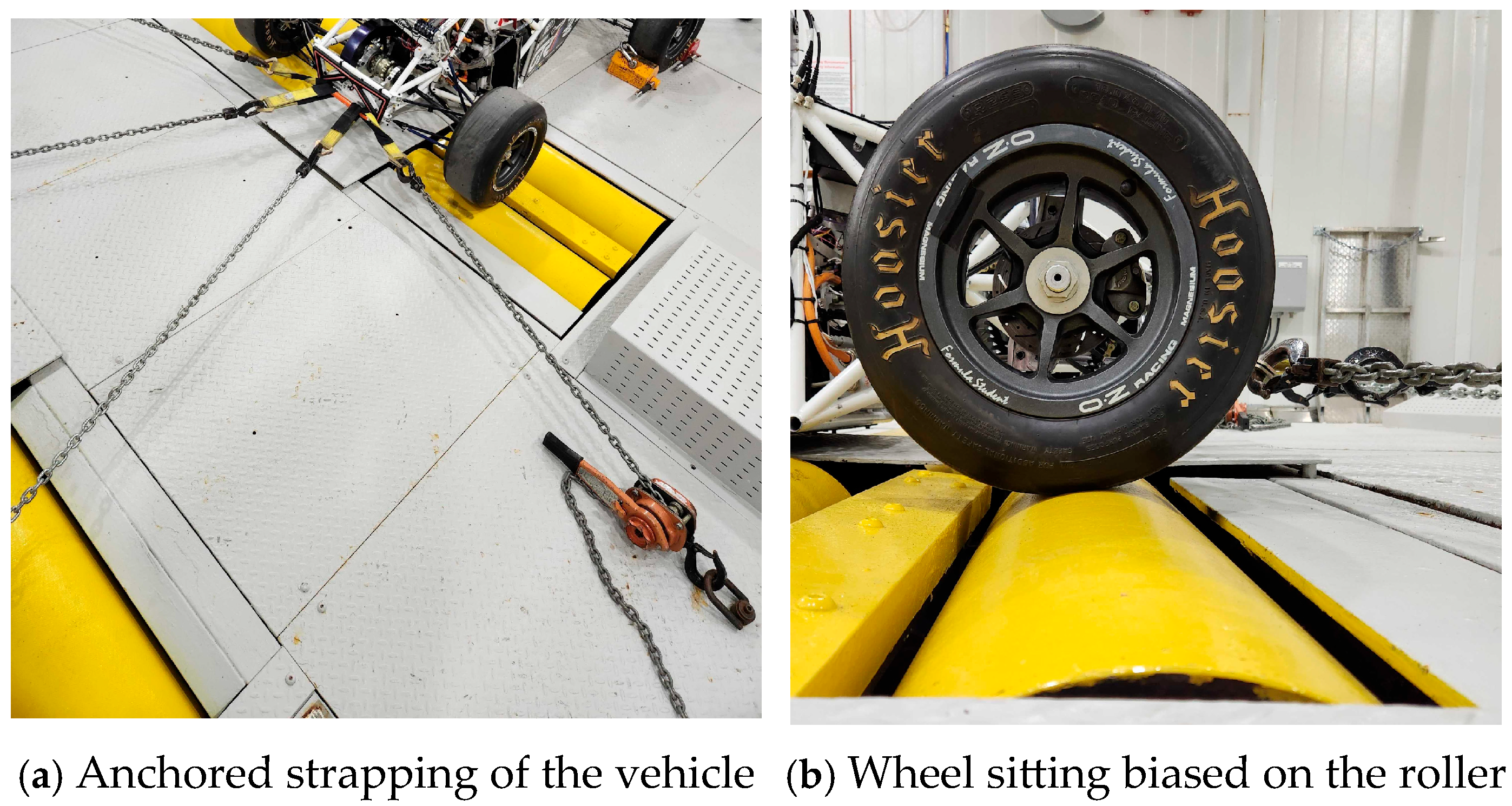
The vehicle was strapped to the dyno in six opposite directions, all pulling from the unsprung mass. The vehicle was set up so that the rear wheels were biased on the front face of the rollers so the vehicle would roll off and away from the rollers in an unsafe event, as seen in Figure 3a,b.

To operate the vehicle, the signals that were otherwise coming from the analog sensors of the driver interface, a bypass were bypassed through a Controller Area Network (CAN) communication. The CAN communication was fed to the motor’s inverter for standardized throttle input profile requests. All operators were placed at a safe distance from the vehicle using this remote setup. Other safety items were also in place, such as an e-stop used to shut down the HV interlock and remove the tractive system voltage from the surrounding environment. To apply a constant road load, the MD-AWD-500 user interface was used to throttle the resistance of the dyno drum. To finish up setting the vehicle on the dyno, a strap loading was used to apply a controlled vertical force on the tires.

Data acquisition was performed through a combination of the systems on the F22 and a separate apparatus used to measure tire slip. All data was collected through CAN communication and a CAN logger on board F22 from CSS Electronics. This allowed the ability to obtain data that was time synchronized, aiding in data validity and usability. Virtual sensors were any data that could be modeled by a combination of other real sensor data, vehicle known values, a mathematical model, and/or a physics model.

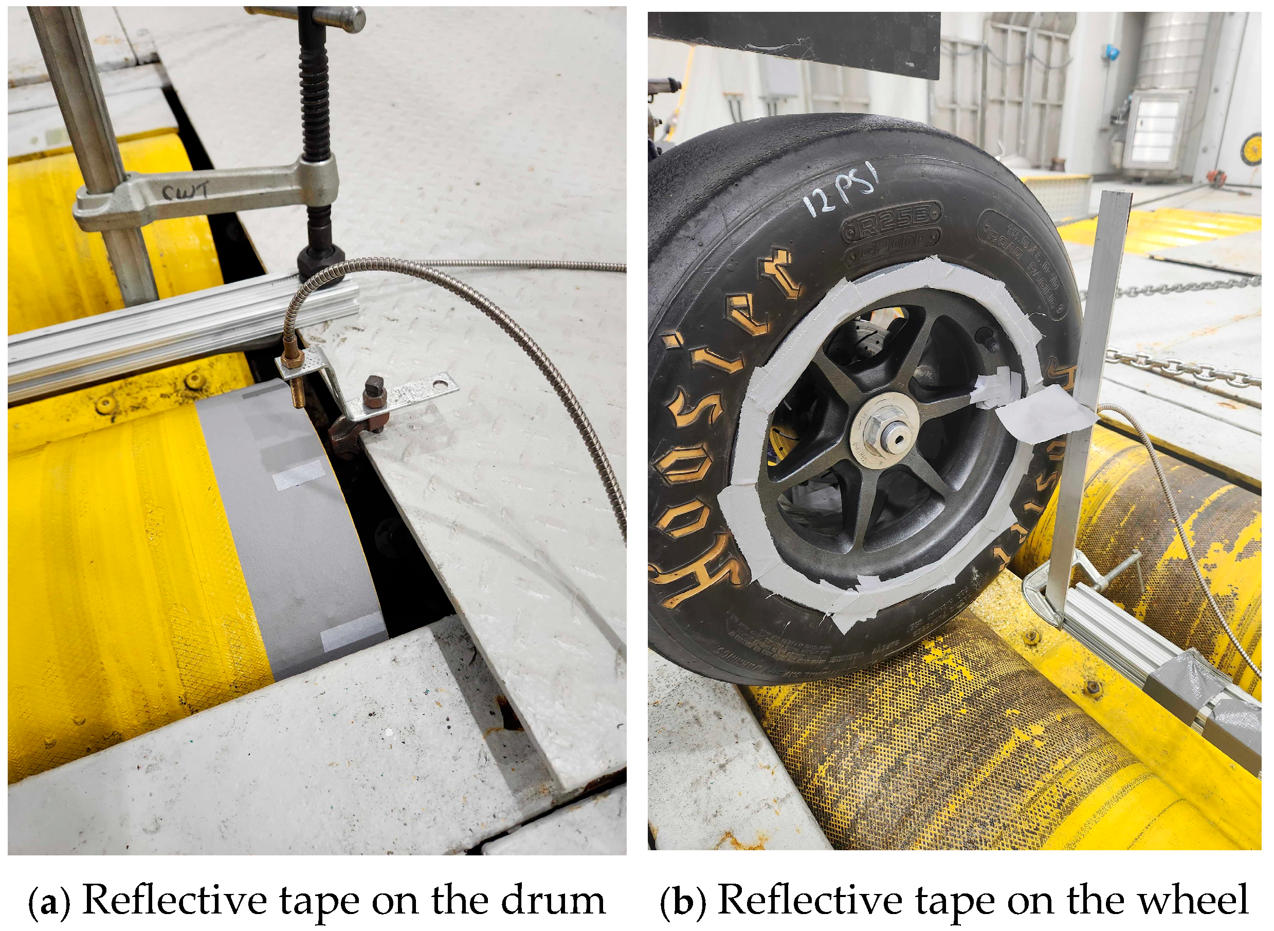
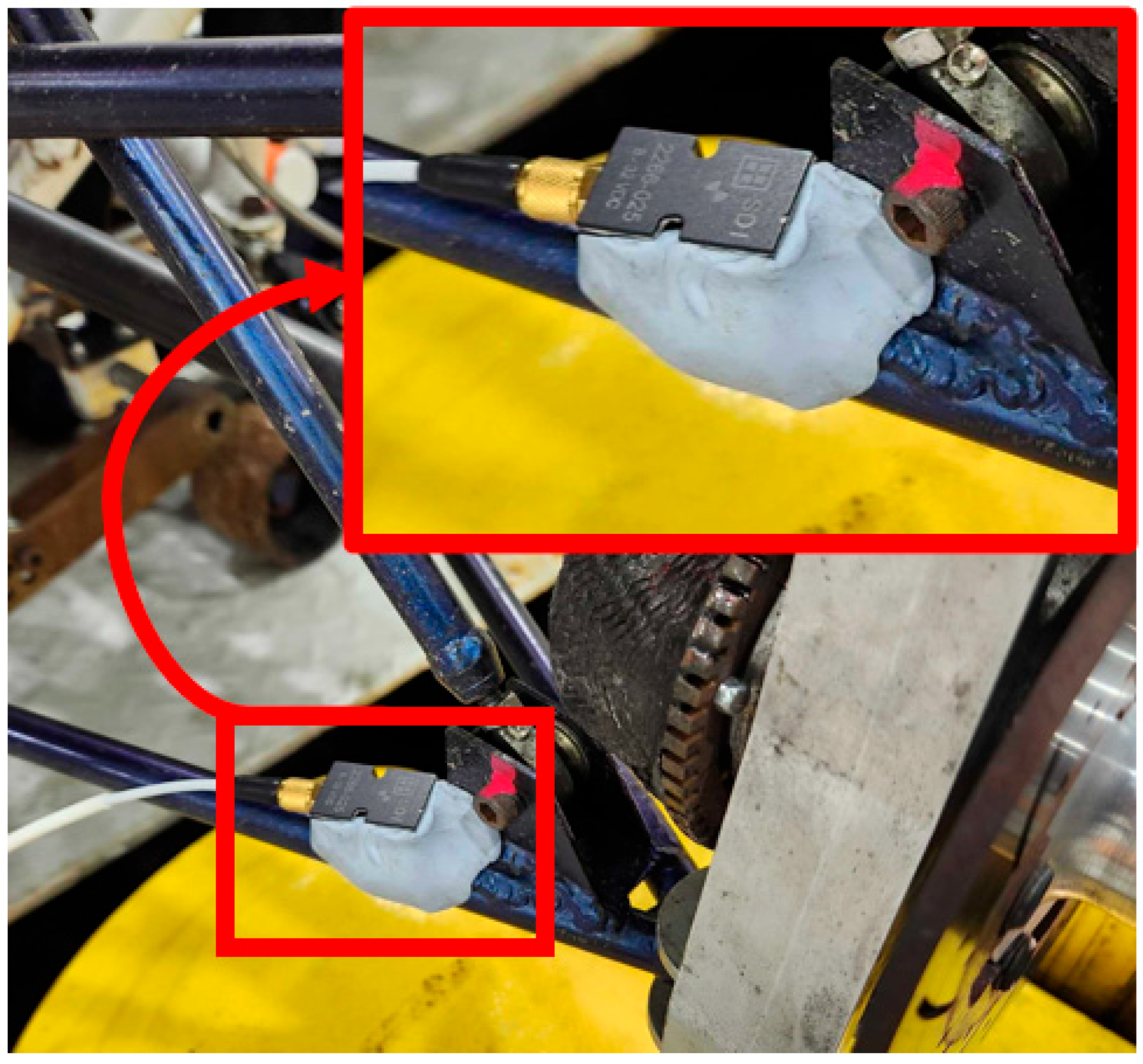
Most of the data related to tire forces were calculated using the outputs from the vehicle motor inverter. Using its calculated torque measurement, various tire parameters and forces would be displayed. The inverter was also able to provide motor speed, which can be used to calculate wheel speed. For additional measurements, the accurate speed of the road and wheel is required. To do this, a CSS digital to CAN module was used along with a reflective pulse sensor to calculate dynamometer drum speed and wheel speed, as in Figure 4. Comparing these relative speeds can be used to determine the slip between the wheel and the road. This could then be used to determine the friction coefficient of the tire and road and monitor any excessive slip.

Vertical loading was a static measurement based on the pretest data, and then adding the additional force calculated via the suspension spring compression. Due to the vehicle not moving on a course, this was sufficient for data collection. Despite this, an accelerometer was also placed at the end of the control arm nearest to the upright and collected vibrational data. This allowed for compensation due to any additional forces introduced by any phenomena like wheel hop related to the kinematic characteristics of the suspension during acceleration, and any imbalance in the driveline. This can be seen in Figure 5.

At the end of every test, the tire was weighed on a high-precision scale with an accuracy of 0.01 g to calculate the tire wear over time. Using a datum weight taken before the test, the amount of tire compound that was shed during testing could also be determined to calculate tire degradation. At the end of testing, the data were presented as a time series for post-processing in Excel and MATLAB R2025a.

2.2. Wear Experiment Setup

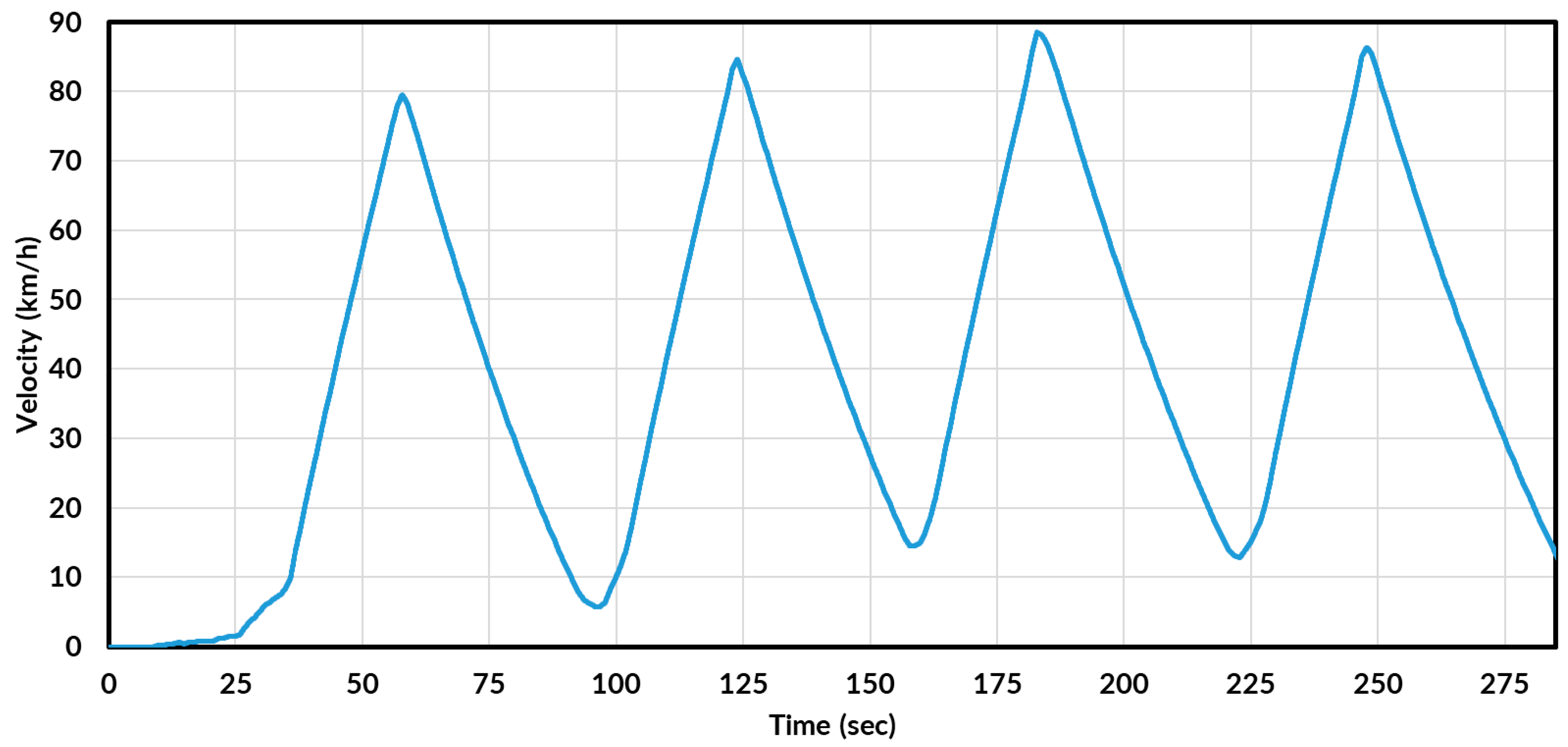
The wear experiment on the dynamometer consisted of three sets of acceleration-deceleration tests. Each test lasted 900 s (15 min), with a predefined testing profile. Between each 900-s set, the batteries were required to charge for approximately an hour. Each experimental Wear Test (WT) in this work will be noted as: Wear Test 1 (WT1), Wear Test 2 (WT2), and Wear Test 3 (WT3). Each wear test used the same testing profile, where one acceleration-deceleration cycle is completed in approximately 60 s. The torqued wheel speed of the tire on the dynamometer is recorded and used as input in the simulations to retain accuracy.

The strapped-down tire load on the dynamometer was measured to be 220 lbs., inflated to 12 psi, and was set up for 0-degree toe, slip angle and inclination angle. The tire was accelerated to approximately 85 km/h longitudinal velocity and decelerated to 15 km/h. This acceleration profile was a common acceleration profile for the FSAE vehicle and was also used to test the limitations of the battery onboard. The experimental velocity output for the WT tire can be seen in Figure 6 for the first 300 s.

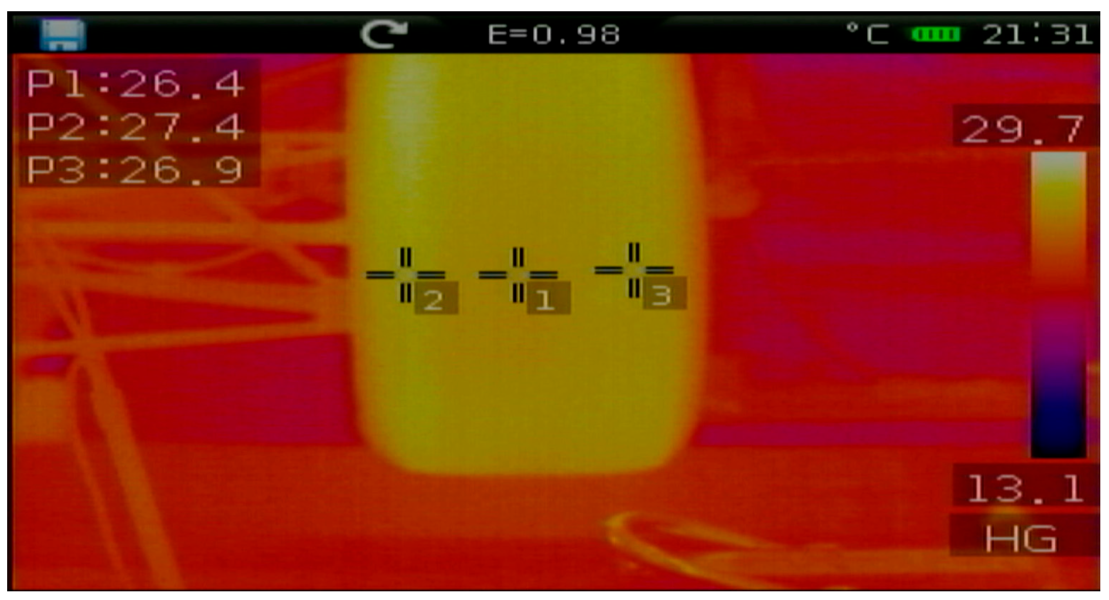
An infrared thermal camera was used to determine the tread temperature of the tire as it rotates on the dynamometer drum. Three measurements of the tire temperature along its width were recorded. Figure 7 shows the tire thermal measurements in °C, where P1 indicates the central tread surface temperature, P2 indicates the inside tire temperature closest to the vehicle chassis, and P3 indicates the outermost tire surface temperature.

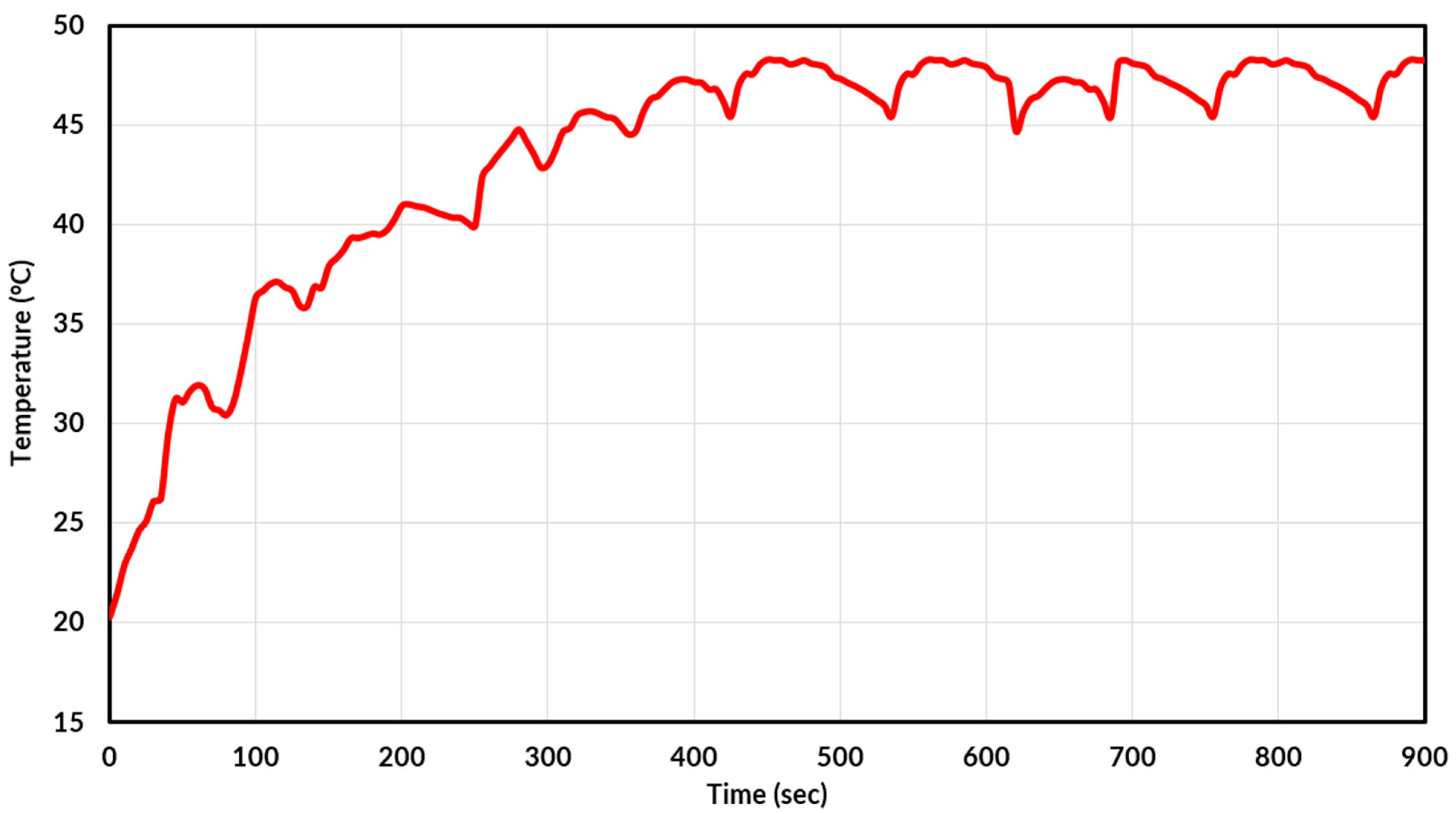
With these measurements, the tread temperature during the tire’s transient acceleration and deceleration loading can be measured. The average tire temperature, which was used for the tread-hardness correlation over time, can be seen in Figure 8. The tread temperature can be seen to follow the velocity profile, where wheel speed and temperature increase together. However, after the first cycle, the temperature is seen to lag behind the wheel speed due to the viscoelastic behaviour of the tire, as also seen in the supporting literature [18]. This is due to the heat in tires being generated from both internal hysteresis and friction at the contact patch. From this heat, the dissipation through conduction, convection, and radiation does not happen instantaneously, leading to temperature drag. At approximately 400 s into the WT runs, the temperature saturates at 51 °C. This temperature relationship is later used in correlation to a tread hardness model for the R25B tire.

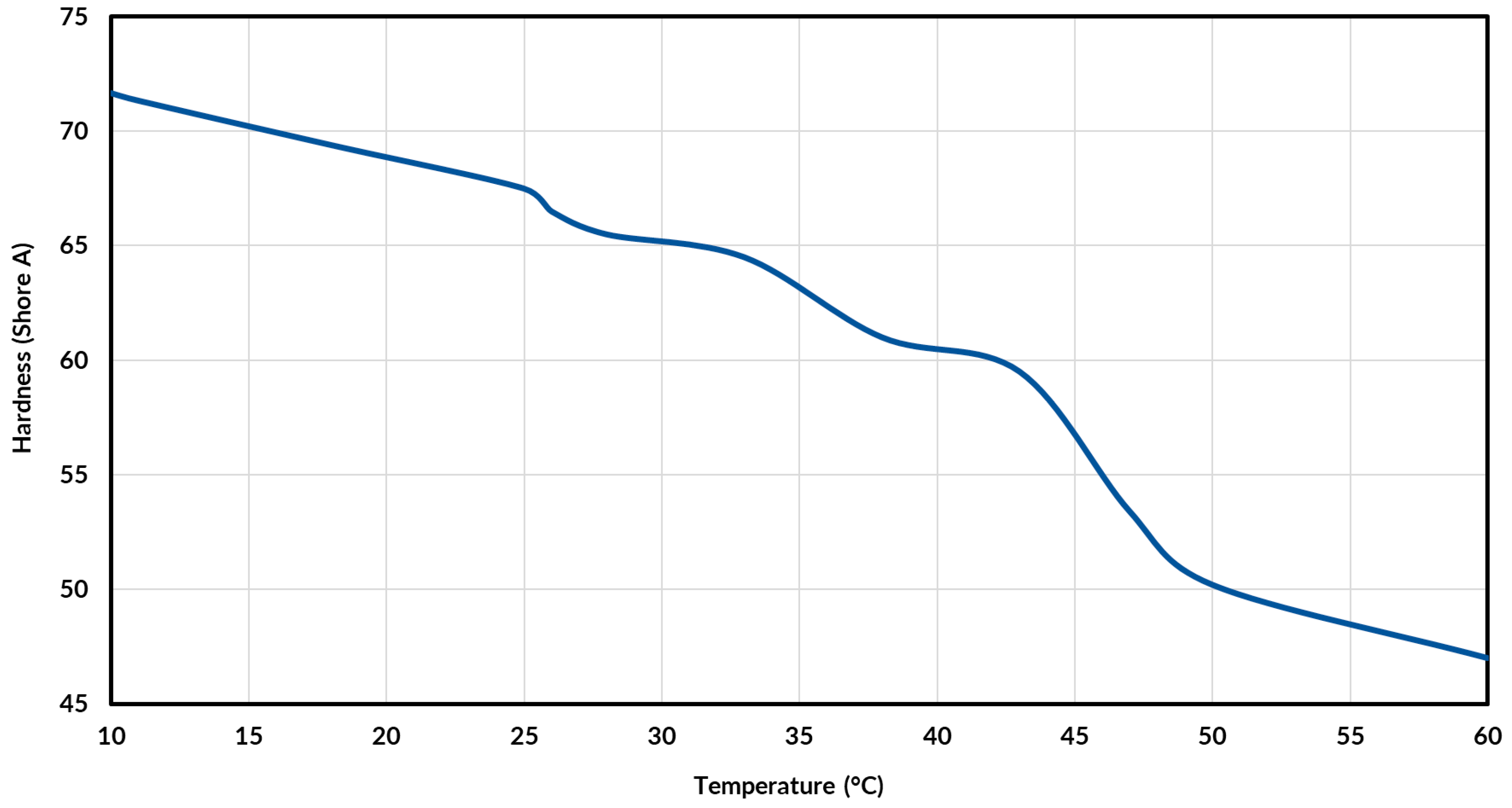
The Shore A hardness durometer was used to measure the hardness of the tread rubber at varying temperatures. The tire was placed into an AES ZBD-908 laboratory oven, heating the tread up to 60 °C. More specifically, the tire tread portion was evenly heated within the oven to closely replicate the tread surface temperature experienced in testing. As the tire cooled to 10 °C, the Shore A durometer was placed against the tire tread to determine its hardness as it cooled. The Shore A hardness can be seen to decrease non-linearly as temperature increases in Figure 9. As tire temperature increases, the tread rubber becomes soft and pliable, hence the decrease in hardness. The same trend for tire rubber can be seen in the literature [19].

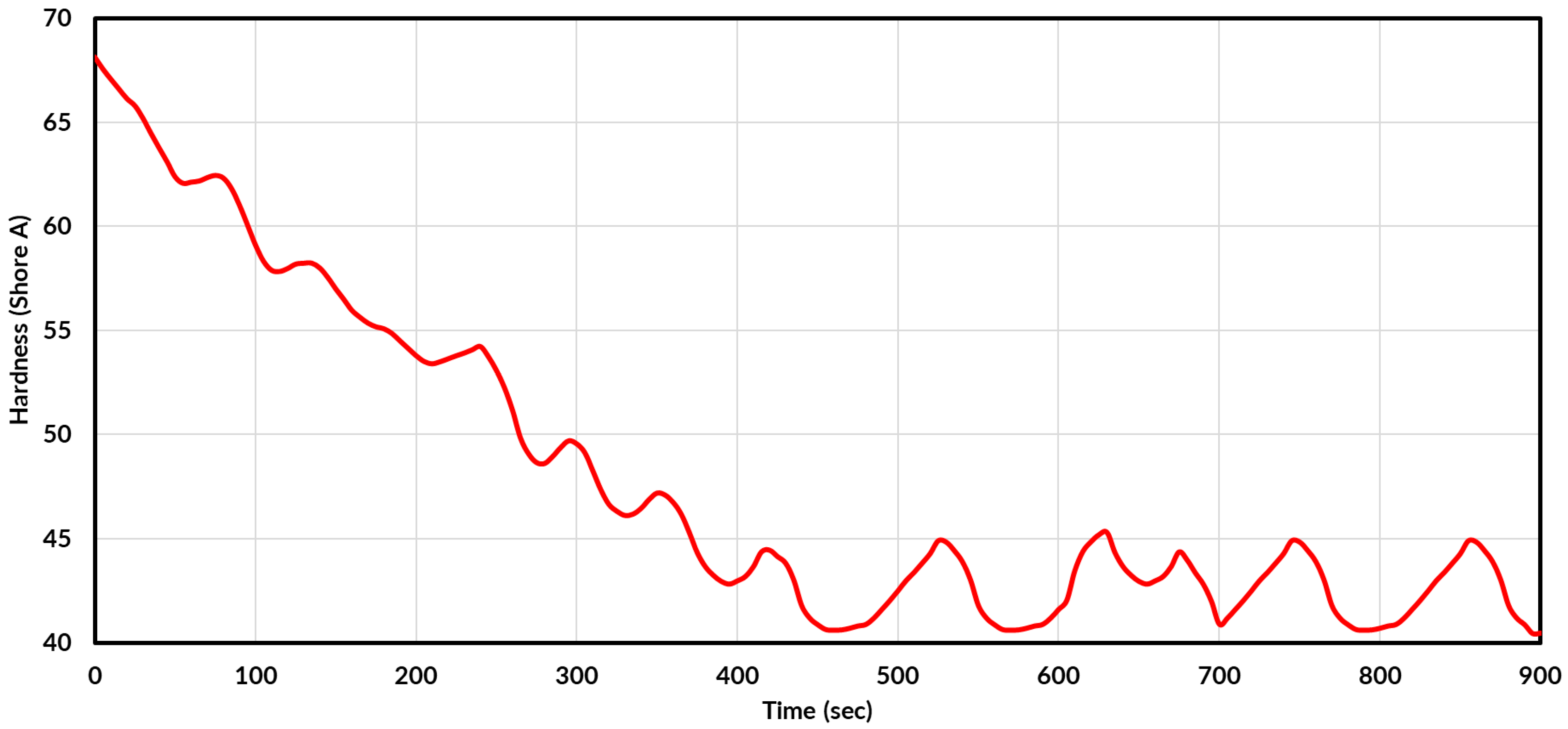
When combining the temperature readings of the tire in Figure 8 and the hardness relationship in Figure 9, the tire’s hardness relative to time and, therefore, velocity can be determined. This is shown in Figure 10, where the hardness of the tread decreases with the WTs acceleration-declaration cycles over time. The hardness can be seen to decrease non-linearly over time, in similar oscillations to those of Figure 8. Then the hardness saturates at approximately 42 Shore A, as temperature saturates at 51 °C. These trends are expected, as the hardness relationship is dependent on the temperature relationship and therefore shares similar oscillations and patterns. This hardness model is then used later in the wear model discussed in the Section 4.

3. Wear Simulation

This section briefly outlines the tire FEA model, its specifications and validation process. More importantly, the wear simulation model is presented.

3.1. FEA R25B Tire Model

The FEA R25B tire is a fully solid three-dimensional model using mainly the Ogden material definition in Virtual Performance Solutions (VPS). To model the Hoosier R25B 18X6.0-10 Tire, the tire was measured in both its external and internal dimensions along with its cross-section to determine its internal construction. The deflated tire dimensions were taken when the tire was recreated in the FEA environment. The sidewall nearest to the bead included an additional layer of nylon ply, increasing the stiffness of the region, and extended towards the mid-section of the tire’s sidewall. The nylon ply and the rubber of the tire were found to be around 3 to 3.5 mm thick in the tread of the tire. To adequately simulate the tire, the material properties of the nylon ply in the longitudinal and lateral directions, and the rubber were implemented into the model. When modeling the tire, the tire was split into five primary parts: the Bead, Lower Bead, Upper Sidewall, Lower Sidewall, and Tread. The direction of these components can be seen in Figure 11. These distinctions allowed for different configurations of materials to achieve a more accurate model of the R25B 18X6.0-10 tire, as seen in Figure 12. The tire model also consists of 10 layers of material. Figure 12b depicts the various parts of the FEA tire model, including its 10 layers. Aside from the bead, there were approximately 3–5 layers of rubber towards the outer wall of the tire. Towards the lower sidewall and lower bead, there were denser concentrations of ply layers, and thus more of the composite and ply material was allocated in those regions. The bead nodes were constrained to a Center of Gravity (COG) node that was located at the symmetric center of the tire in all axes. This tire center COG included the properties of the rim, including materials and density.

The Ogden tire parameters for the FEA model can be seen in

Table 1. Tire material Ogden Parameters for VPS FEA model.

	${\mathit{\mu }}_1$	${\mathit{\mu }}_2$	${\mathit{\alpha }}_1$	${\mathit{\alpha }}_2$
Composite—Longitudinal	0.1038	−0.2164	3.85	−7.498
Composite—Lateral	0.103	2.838	0.6284	2.131
Ply—Longitudinal	3.28	2.85	4.16	3.59
Ply—Lateral	−1.96	−0.695	−7.33	−8.21
Rubber—Tread	−0.00183	−0.144	−9.62	-5.8
Rubber Sidewall	0.898	−0.00733	1.25	−7.04

, obtained through uniaxial tensile tests. The Ogden material definition was used to define the tire materials and hyperelastic tread materials. This Ogden hyperelastic model is a linear combination of strain invariants, where the principal stretches are independent variables that are also subject to an incompressibility constraint. As mentioned, the Ogden hyperelastic model fits rubber and soft material effectively and is versatile, as it can degenerate and represent Neo-Hookean and Mooney-Rivlin material models. The Ogden strain energy function, as used in the VPS FEA environment, can be seen in Equation (1).

$${\overline{W}}^0\left(\overline{C}\right)={\sum }_{A=1}^3 {\sum }_{i=1}^{N_{\mathrm{shear} }} 2{\displaystyle \frac{{\mu }_i}{{\alpha }_i}}\left({\overline{\lambda }}_A^{{\alpha }_i}-1\right)+{\sum }_{i=1}^{N_{\mathrm{vol} }} {\displaystyle \frac{1}{D_i}}(J-1{)}^{2i}$$

(1)

where ${\lambda }_A$ are the eigenvalues of the deformation gradient matrix, $J$ is the determinant of the deformation gradient matrix, $U^0$ and ${\overline{W}}^0$ are volumetric and volume-preserving portions of the stored energy function, and ${\mu }_i$ and ${\alpha }_i$ are material parameters and fitting components for the Ogden model.

The viscoelastic properties of the tread rubber were captured through a stress relaxation test using the TA Instruments Q800, as seen in Figure 13. The stress relaxation test was used to determine the tread rubber’s viscoelastic effect by stretching the rubber to various strains (20%, 60%, 80%) and observing the stress response over time. The captured stress relaxation response, as in Figure 13, is directly input into ESI VPS 2023.

To validate the tire model, a vertical stiffness test was performed within VPS FEA, where a simulated stiffness was found to be 97.449 N/mm. This yielded a 2.702% error with a measured stiffness of 100.173 N/mm at 0-degree camber. A footprint test was also simulated in VPS FEA, where a simulated footprint yielded 13,665.672 mm². The measured footprint was 13,650 mm², resulting in a 0.115% error. Finally, a Rolling Resistance Coefficient (RRC) test was performed at different speeds with FEA as seen in Figure 14. The largest error found against experimental data was 3.45% at 72 km/h. The R25B tire model shows comprehensive agreement compared to its experimental test results.

3.2. Wear Simulation Model

To determine wear in the simulation environment, Archard’s wear theory is implemented in conjunction with MATLAB. First, the FEA model is loaded to 220 lbs. of vertical load on the dynamometer, and inflated to 12 psi as in Figure 15. Then the required torque drives the tire to accelerate to a maximum longitudinal velocity of 85 km/h. The tire follows the same velocity profile as the driven tire shown in Figure 6, using an imposed rotational velocity load. The contact used between the tire and drum is the non-symmetric master-slave node-to-segment-oriented contact. The loading is applied to the tire center using the Multiple-Nodes-to-One-Node (MTOCO) constraint, tying the bead nodes to one node to the arbitrary rim center. The constraint equations that define the MTOCO can be seen in Equations (2) and (3).

$$\overrightarrow{U}\left(n_d\right)=\overrightarrow{U}\left(n_i\right)+\overrightarrow{\theta }\left(n_d\right)\wedge \overrightarrow{d}$$

(2)

$$\overrightarrow{\theta }\left(n_d\right)=\overrightarrow{\theta }\left(n_i\right)$$

(3)

where $\overrightarrow{U}\left(n_d\right)$ and $\overrightarrow{U}\left(n_i\right)$ are the displacement vectors of the dependent nodes and independent nodes, respectively, $\overrightarrow{\theta }\left(n_d\right)$ and $\overrightarrow{\theta }\left(n_i\right)$ are the rotation vectors of the dependent nodes and independent nodes, respectively, and $\overrightarrow{d}$ is the vector from $n_i$ to $n_d$.

Within the simulation, the required contact pressure, contact area, interface velocity, and consequently the friction energy developed are obtained. The friction energy and the tread temperature are then correlated within MATLAB accordingly, and a wear ablation value is determined. Archard’s wear theory was implemented to determine the wear of the R25B tire. The wear model can be seen in Equation (4).

$$\dot{q}={\displaystyle \frac{k}{H}}PA\dot{\delta }$$

(4)

where $\dot{q}$ is volumetric material loss, k is a wear coefficient, H is material hardness, P is contact pressure, A is contact area and $\dot{\delta }$ is contact slip rate. The product of the contact terms: P, A and $\dot{\delta }$, is the contact patch frictional dissipation energy rate.

Traditionally, Archard’s wear theory functioned well for constant area, constant pressure and constant speed applications. However, further efforts have shown Archard’s wear theory to be effective in dynamic/transient situations. One study applied an exponential constant to the contact terms to adjust for the exponential characteristics of rolling resistance with speed [16]. However, it is more effective to develop a proper model, with validated rolling resistance up to the speeds required for the wear model, like this R25B FEA model. Developing a high-fidelity model that is validated in multiple domains will ensure an accurate frictional dissipation rate from the contact patch output within the FEA environment. Additionally, a R25B tread hardness model will be used in tandem with Archard’s wear to effectively measure wear alongside tread temperature. A modified Archard’s wear model was proposed to estimate wear as in Equation (5).

$$\dot{q}={\displaystyle \frac{K}{\frac{\partial H}{\partial t}}}·{\displaystyle \frac{\partial {\dot{E}}_{fric.diss.rate}}{\partial t}}$$

(5)

where ${\displaystyle \frac{\partial H}{\partial t}}$ is the change of tread hardness of the R25B tire with time, and ${\displaystyle \frac{\partial {\dot{E}}_{fric.diss.rate}}{\partial t}}$ is the change of contact friction dissipation rate over time. The ${\displaystyle \frac{\partial {\dot{E}}_{fric.diss.rate}}{\partial t}}$ ensures that Archard’s wear functions with under transient maneuvers, and ${\displaystyle \frac{\partial H}{\partial t}}$ ensures that the tread hardness captures the differences due to temperature over time.

Once the wear ablation is determined, or wear reduction, the nodes in the tread section only are then uniformly reduced, and the simulation continues again for further simulation cycles. The tread is linearly reduced in the vector of the tread element towards the tire center. The process repeats for the required number of cycles to predict wear. The more time, simulation cycles, and frequency of remeshing, the more detailed the wear model, but the more computationally expensive it is. The ablation process to reduce the tread nodes utilized VPS FEA’s CATGEN export/import functions. The CATGEN export control generates a dedicated export file during a simulation or run. This output file allows the modification of nodes, particularly the outer-tread nodes, and then continues the simulation through CATGEN import. This feature outputs many applications, including: sub-modeling displacement, velocity, mapping stress and strain, geometrical mapping modification, complex remeshing, and much more. The import feature uses a temporal interpolation algorithm. In general, the simulation procedure for wear can be seen in Figure 16.

4. Simulation Results and Validation

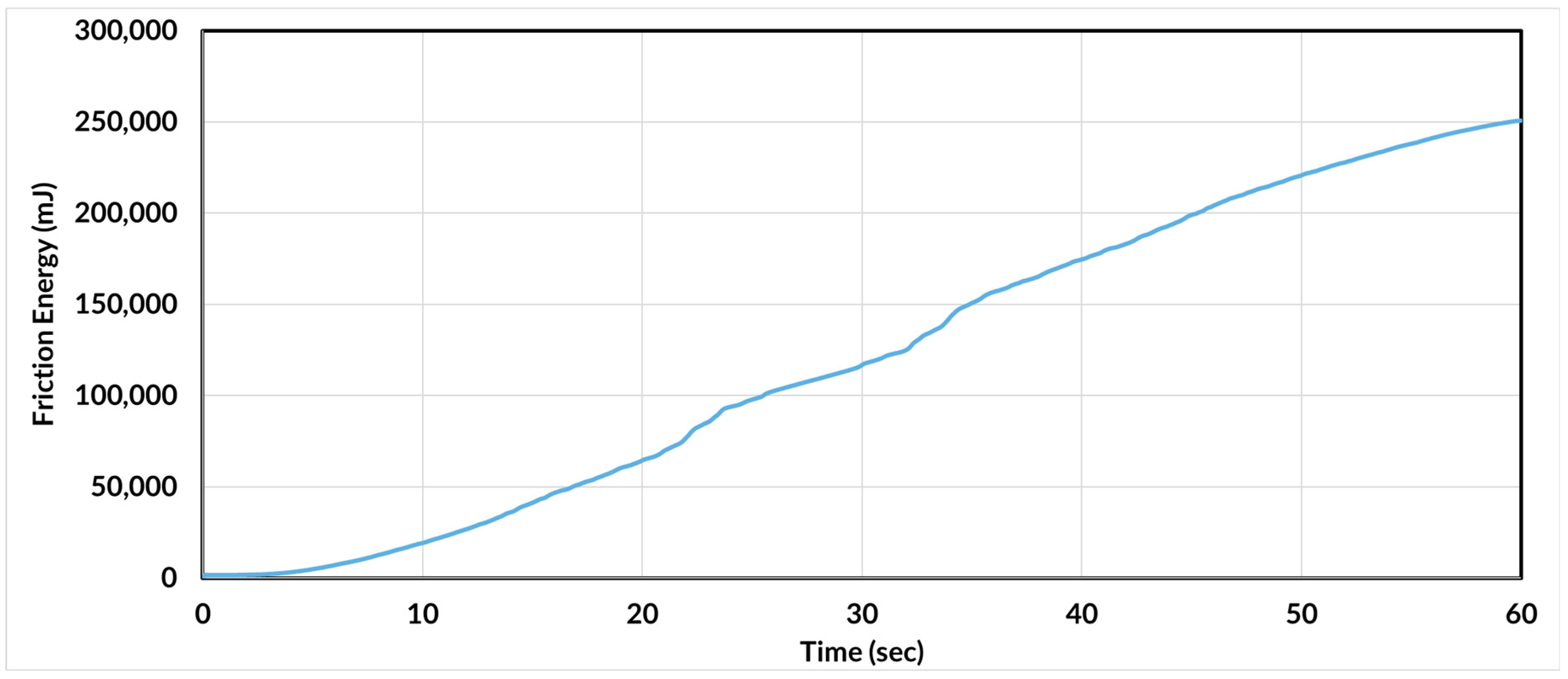
Generally, the friction energy dissipated at the tire contact can be seen to follow an exponential trend, as in Figure 17. This shows the friction energy rate for the reference tire simulation model with no wear, hence a datum. The friction energy can be seen to increase slightly exponentially during acceleration up to 30 s. As the tire decelerates, the friction energy continues to increase; however, it saturates at the 30 s mark, and saturates further near the end of deceleration at 60 s.

To replicate the tire wear from experiments, 12 wear reductions in the tire tread were simulated according to the implemented wear process. The simulated tire in each wear step lasted for 180 s to 225 s, depending on wear rate. Each wear step reduced the radius by approximately 0.001 mm, corresponding to a volume reduction of approximately 250 mm³ each step. This was found to produce a wear model that was more than sufficient to accurately capture the wear of this model. However, it should be noted that more aggressive and instantaneous tire wear will require more wear steps to accurately capture the mass loss phenomena. Each wear step is a reduction of approximately 0.001 mm for the outer tread layer within the FEA tire model. In terms of volumetric losses, outer tread elemental volume is clearly presented in

Table 2. Outer layer tread elements volume for each wear step.

Wear Step	Outer Tread Layer Element Volume (mm3)
0	175,675
1	175,424
2	175,193
3	174,962
4	174,731
5	174,489
6	174,248
7	174,007
8	173,776
9	173,545
10	173,314
11	173,083
12	172,852

. For clarity, as aforementioned, the ablation is dependent on the friction energy dissipation, tread hardness and speed. Additional considerations for ablation are the nodes connecting the sidewall to the central tread portion. When reducing the tread layer, the connecting nodes and consequent elements are affected towards the sidewall.

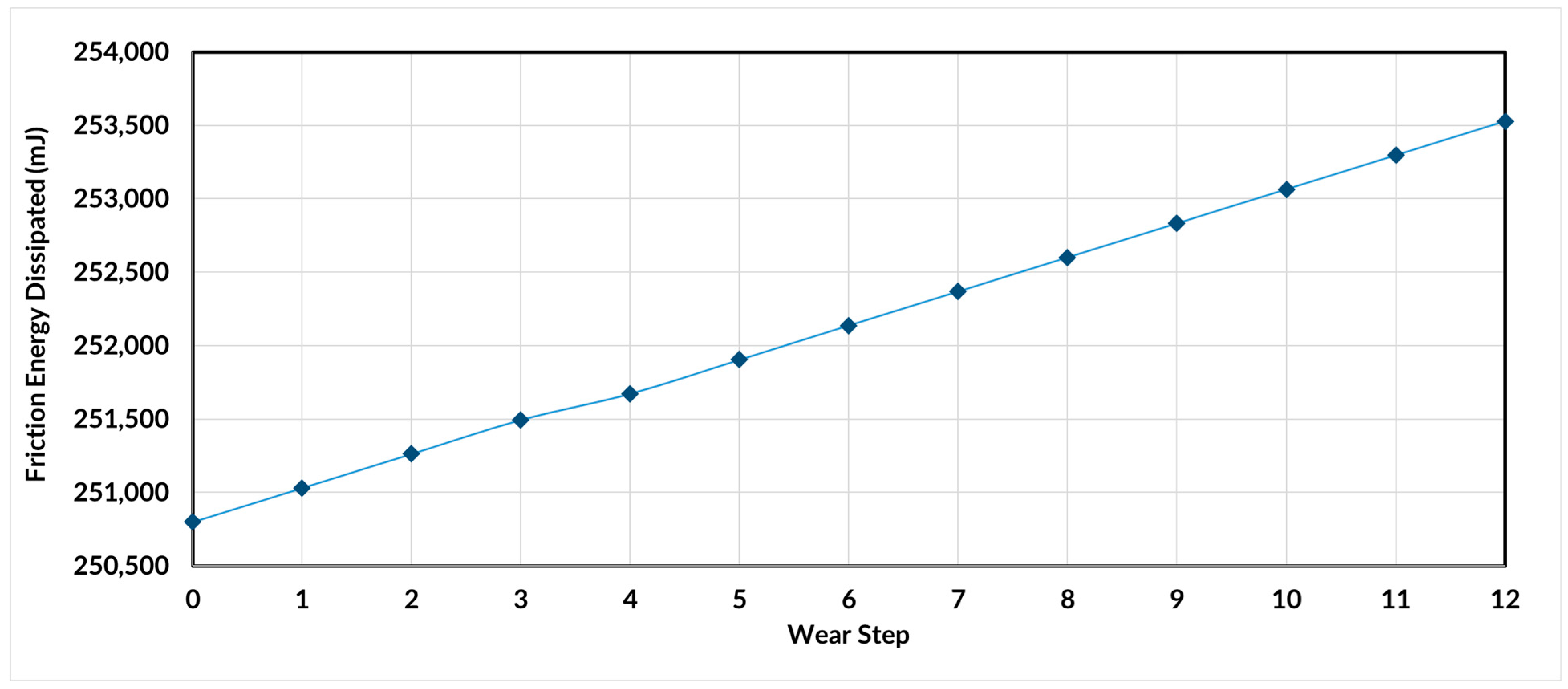
Figure 18 presents the friction energy dissipation difference of the datum or reference tire model with each worn tire model, denoted as ‘Step 1’, ‘Step 2’, and so on. When comparing the dissipated friction energy of different wear step tire models to the reference datum plane, wear step 12 shows the largest difference of 2728.031 mJ. For clarity, the difference between the reference energy rate and the step 1 model energy rate is minuscule, in that it is presented closest to 0 mJ. However, the reference energy rate is heavily different when the model reaches wear step 12, showing a difference of 2728.031 mJ at the end of a cycle. It is observed in simulation that each wear step tire model increases linearly in friction energy dissipation per cycle, with the exception of wear step 4. In step 4, the slightest of changes for the connecting nodes between the tread and sidewall altered the linearity of friction energy dissipation for a cycle. This is more clearly noticed in Figure 19, where there is a very small dip in friction energy for the otherwise linear trend.

Figure 19 shows the friction energy for the span or an acceleration-deceleration cycle for every wear step model. This suggests that for the wear amount of the tire, the friction energy linearly increases with every wear step. The general pattern of this is as expected, due to the tire maintaining the same speed with a reduced tread, there will be a slight increase in rolling resistance for the wear occurring.

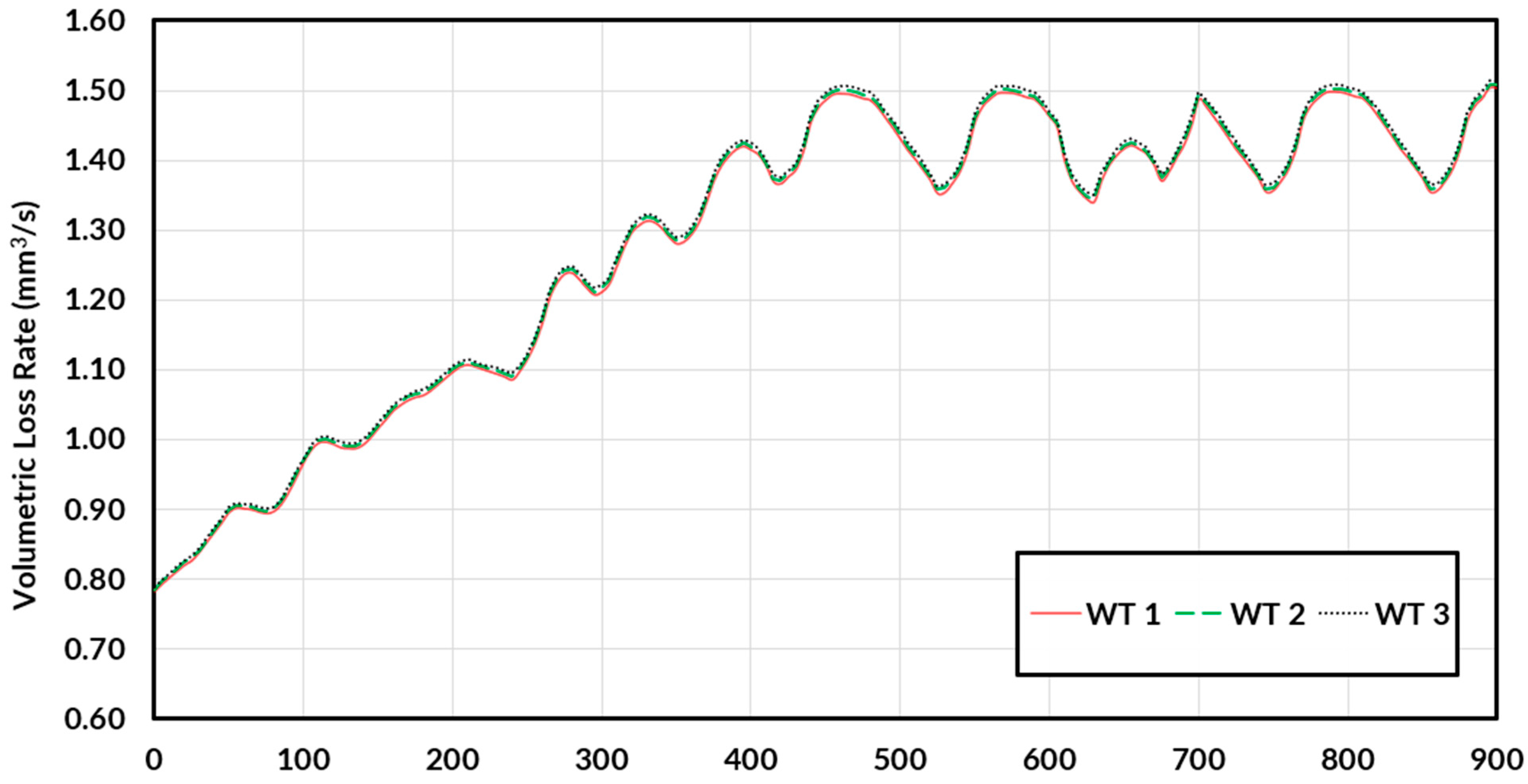
Using the modified Archard’s wear equation, the volumetric loss rate, $\dot{q}$ was determined for the full 900-s simulation as seen in Figure 20. Each 900-s simulation can be seen through WT 1, WT 2, and WT 3 with their respective $\dot{q}$ values. WT 1 underwent 5 wear steps, WT2 and WT3 underwent 4 wear steps each, where each wear step varied the friction energy rate slightly. Due to Archard’s wear theory, the increasing friction energy rate yields a slightly higher volumetric loss rate as they are directly correlated. Therefore, while the $\dot{q}$ can be seen to be quite similar in linear regions, but it can also differ at its peaks after accelerating for varying WT. As the tire wore more over time, a higher $\dot{q}$ can be observed when comparing WT 1, WT 2 and WT 3. The difference was observed to be more prominent in later times for each wear step as the first 200 s showed very similar results between WTs. A major factor that determines the $\dot{q}$ is the tire’s thermal generation at the tread. The hardness value in the wear theory used was determined using a temperature-hardness correlation from Figure 8 and Figure 9. The temperature of the tread surface as determined by the experimental thermal measurements, can be seen to contribute to the general trend of $\dot{q}$ with time in an inverse relationship.

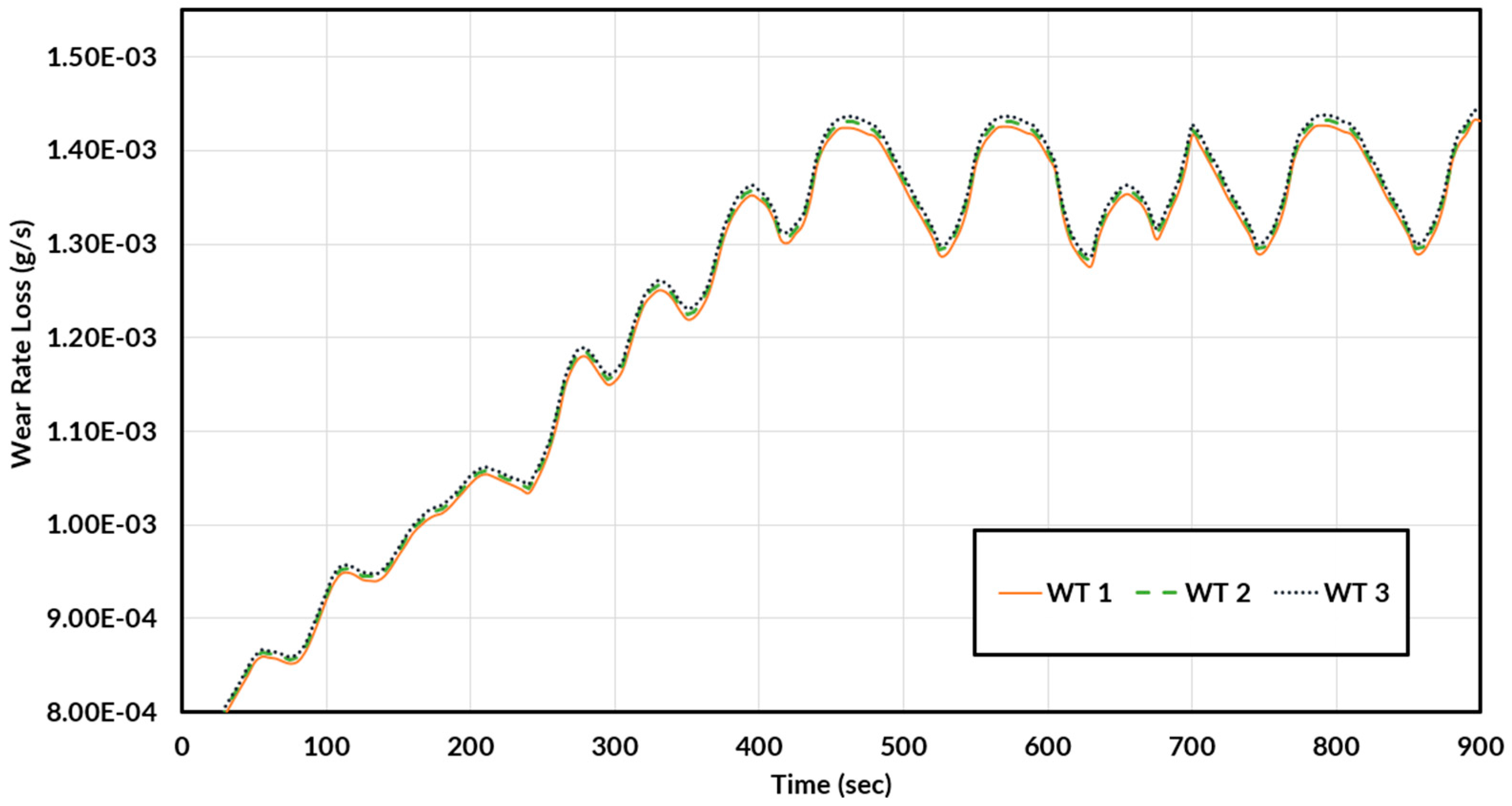
Figure 21 presents the tread wear rate loss between each WT. This is the result of the product between $\dot{q}$ and tread rubber density, 953,228.8 g/m³. In post-processing for calculating $\dot{q}$, a time step of 5 s was used. For every 5 s, a wear rate loss is determined as seen in Figure 21. When taking the product of the instantaneous wear loss rate in its time span, the wear mass value can be predicted.

When looking at the actual tire wear mass over time from simulation as presented in Figure 22, each WT shows a slight exponential increase of tire wear with time, heavily influenced by the temperature increase of the tire tread and slightly correlated by the difference in friction energy. Between the WTs, the differences at the beginning show negligible wear differences; however, the wear differences are more apparent after accumulating some temperature at the tread compound. 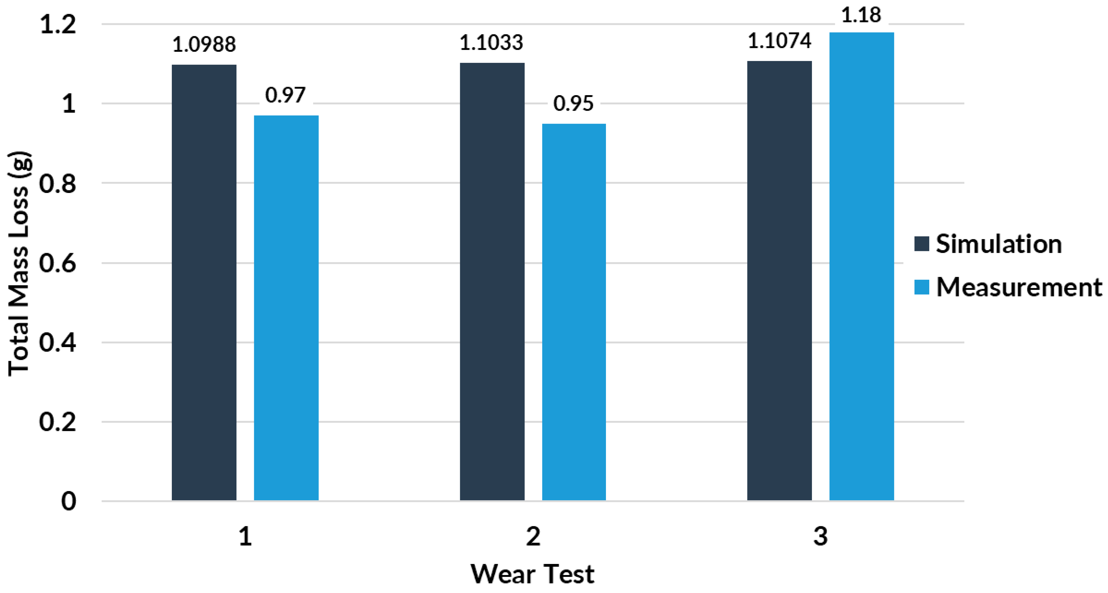Alike $\dot{q}$, the wear mass difference can be seen to be more apparent later in the simulation. As it is difficult to show the variation between the simulated WTs, the total mass loss can be seen clearly in Figure 23.

The tire wear mass for WT 1, which includes 5 wear steps, was found to be 1.0988 g, WT 2, including 4 wear steps, was found to be 1.1033 g and WT3, including 4 wear steps was 1.10741 g. WT 1 and WT 2 differed by 0.00454 g, and WT2 and WT 3 differed by 0.00407 g of tire wear loss. In experimental measurement, there is no distinct trend between the mass loss per WT. Between WT 1 and WT 2, there was only a 0.02 g difference in mass loss, however, a 0.23 g difference can be seen between WT 2 and WT3, which may suggest a mass loss increase correlation with wear.

A total wear loss of 2.95983 g was seen between the WT simulations with an estimated wear coefficient of $2.8162\times {10}^{-7}$. The experimental tests yielded a wear mass loss of 3.10 g, resulting in a 4.5216% error, which shows agreement between measurements and simulation. Between WT 1 and WT 2, the total mass loss can be seen to differ from experimental measurements. However, including WT 3, the trends do show an overall increase of total mass loss with each progressing WT. The small difference between WT 1 and WT 2 in the experimental tests may be attributed to temperature changes between the garage door opening. Where the outdoor ambient temperature and the dynamometer area inside the facility may have caused a slight difference in mass measurement. Additionally, there was a significant accumulation of paint from the steel roller by the end of WT 3 in experiments that may have contributed to the significant increase in mass by WT 3. In the experiment, as the tire wore more, the tread surface may have increased in roughness. In parallel with significant temperature changes over time, the tire tread was seen to accumulate more paint as the wear tests continued. The paint on the tire can be seen in Figure 24.

The wear model can be seen to be heavily influenced by temperature and tread surface hardness, and for the wear amount simulated, slightly influenced by friction energy rate. This work suggests that there is an exponential increase in wear mass loss over time that is dependent on the friction energy rate, and therefore tread hardness, contact area, contact pressure and speed. As this study shows slight increases in friction dissipation rates and mass loss for a moderate amount of tire wear; the data suggests a more significant, exponential difference were the tire to show excessive wear. For future work, other velocity profiles can be used to observe the impact of varying maneuvers to tire wear using the same model. This model can also be implemented for other tires provided that an adequate FEA model is developed, and tread hardness for varying temperatures are obtained. Following this, for more instantaneous wear applications a mesh sensitivity analysis will be required. High acceleration loads will deform the elements at the contact patch in more extreme manners compared to those found in this study.

5. Conclusions

This study presents the development of an FEA tire model capable of estimating the wear in transient maneuver scenarios. The FEA wear model built within VPS is a fully solid model, equipped with the Ogden material definition. In conjunction with MATLAB and excel, a modified Archard’s wear theory is applied using a temperature-dependent hardness model and velocity-dependent wear rate. The hardness was obtained at different temperatures of the tire tread, resulting in a hardness-temperature correlation. In combination with a velocity-temperature relationship, a hardness-velocity relationship was established. Using this with the modified Archard’s wear theory, a wear process was built using VPS FEA 2023, MATLAB R2025a, and Excel. The simulated wear model suggested that it is highly dependent on the temperature-hardness relationship, more so than the differences in friction energy rate. The wear mass rate simulated showed an exponential increase with time for each of the WT, whereas the experimental results show a slight increase of wear mass loss between WTs. The simulated wear mass loss was found to be 2.95983 g, compared to a measured mass loss of 3.10 g yielding an agreeable 4.5216% error. Overall, this study suggests that the modified Archard’s wear theory and custom tire model developed from in-house materials testing showed promising results.