An Integrated Mechanical Fault Diagnosis Framework Using Improved GOOSE-VMD, RobustICA, and CYCBD

Abstract

Rolling element bearings serve as critical transmission components in industrial automation systems, yet their fault signatures are susceptible to interference from strong background noise, complex operating conditions, and nonlinear impact characteristics. Addressing the limitations of conventional methods in adaptive parameter optimization and weak feature enhancement, this paper proposes an innovative diagnostic framework integrating Improved Goose optimized Variational Mode Decomposition (IGOOSE-VMD), RobustICA, and CYCBD. First, to mitigate modal aliasing issues caused by empirical parameter dependency in VMD, we fuse a refraction-guided reverse learning mechanism with a dynamic mutation strategy to develop the IGOOSE. By employing an energy-feature-driven fitness function, this approach achieves synergistic optimization of the mode number and penalty factor. Subsequently, a multi-channel observation model is constructed based on optimal component selection. Noise interference is suppressed through the robust separation capabilities of RobustICA, while CYCBD introduces cyclostationarity-based prior constraints to formulate a blind deconvolution operator with periodic impact enhancement properties. This significantly improves the temporal sparsity of fault-induced impact components. Experimental results demonstrate that, compared to traditional time–frequency analysis techniques (e.g., EMD, EEMD, LMD, ITD) and deconvolution methods (including MCKD, MED, OMEDA), the proposed approach exhibits superior noise immunity and higher fault feature extraction accuracy under high background noise conditions.

1. Introduction

Industrial machinery, as a cornerstone of modern industrial production, has played a pivotal role in driving industrial progress, improving production efficiency, and reducing operational costs. In various manufacturing processes, industrial machinery enables precise and efficient production, thereby enhancing product quality and consistency. Rolling bearings, as critical transmission components in industrial machinery, significantly impact the performance and reliability of the entire mechanical system. These bearings support crucial functions such as load bearing, rotational movement, and friction reduction, and their health status is directly correlated with the overall performance and lifespan of the machinery. Therefore, timely and precise fault diagnosis of rolling bearings is crucial to maintain the stable operation of industrial machinery, minimize downtime, and optimize production efficiency. By detecting faults early, maintenance costs can be reduced, and potential damage to other components can be prevented, ensuring the longevity and reliability of the entire mechanical system.

During continuous operation, rolling bearings face numerous challenges such as fatigue accumulation, material wear, and changes in lubrication conditions, all of which can lead to performance degradation and even failure. Under faulty conditions, the vibration characteristics of bearings undergo significant changes, manifested in complex and varied vibration signals that contain abundant fault characteristic information. Therefore, an in-depth analysis of these vibration signals becomes a crucial pathway to reveal the health status of bearings, predict, and diagnose potential faults. Traditionally, vibration signal analysis has relied heavily on classical methods such as the Fourier Transform and its variants [1,2], the Wigner–Ville Distribution [3,4], and the Wavelet Transform [5,6,7]. These methods possess a solid foundation and extensive applications in signal processing, but gradually reveal limitations when dealing with bearing vibration signals exhibiting significant nonlinearity and nonstationarity, making it difficult to fully capture transient features and time-varying patterns within the signals. In light of this, academia and industry have actively explored more advanced adaptive time–frequency analysis methods to enhance the accuracy and efficiency of fault feature extraction. In recent years, adaptive techniques such as Empirical Mode Decomposition (EMD) [8,9], Ensemble Empirical Mode Decomposition (EEMD) [10,11], Local Mean Decomposition (LMD) [12,13], and Intrinsic Time-Scale Decomposition (ITD) [14,15] have emerged. These methods do not require predefined basis functions and can flexibly adapt to complex signal variations, effectively extracting intrinsic mode components that reflect the essential characteristics of the signals. While these methods have demonstrated certain advantages in rolling bearing fault diagnosis, there is still room for further improvement.

Variational Mode Decomposition (VMD) [16], as an emerging time–frequency analysis method, has demonstrated superior performance in vibration signal processing due to its excellent noise robustness, clarity of mode decomposition, and computational efficiency. By solving the optimal solution of a variational problem, VMD achieves adaptive segmentation of signals in the frequency domain, providing a more precise and effective technical approach for fault diagnosis. Z. Jin et al. [17] proposed a train bearing fault diagnosis method based on VMD and an improved Convolutional Neural Network (CNN). This method decomposes signals using VMD to eliminate noise and then utilizes an optimized CNN to enhance classification accuracy. Experimental results show that this method achieves high fault diagnosis accuracy, providing an effective solution for bearing fault diagnosis. Y. Yang et al. [18] introduced a method for extracting rolling bearing condition features based on VMD and Improved Envelope Spectrum Entropy (IESE). Initially, VMD is applied to decompose the bearing vibration signals into multiple Intrinsic Mode Functions (IMFs). Subsequently, the envelope spectrum entropy of each IMF is calculated, and the original feature set is reconstructed through these calculations. Then, Joint Approximate Diagonalization of Eigenmatrices (JADE) is employed to fuse the feature set, yielding a new feature set. Finally, a Support Vector Machine (SVM) is utilized to train and test the new feature set for bearing condition identification. Experimental validation indicates that this method outperforms other approaches in feature extraction. J. Zhou et al. [19] presented a novel rolling bearing fault diagnosis method based on the Whale Gray–Wolf Optimization Algorithm (WGWOA) combined with VMD-SVM. This method utilizes WGWOA to optimize VMD for signal decomposition and feature extraction, followed by SVM for fault classification. Experimental results demonstrate that this method performs exceptionally well on multiple datasets, achieving high fault diagnosis accuracy and outperforming traditional methods, thereby providing an effective solution for rolling bearing fault diagnosis. However, two critical parameters in the VMD decomposition process are the modal component and penalty factor [20,21], both of which are flexible and can be adjusted according to specific needs, significantly impacting the decomposition results. Therefore, how to reasonably select and adjust these parameters poses a significant challenge in VMD applications. Addressing this optimization problem, the GOOSE algorithm (GOOSE) proposed in early 2024 offers a novel and effective solution [22]. Inspired by the behavior of goose flocks in nature, GOOSE is a metaheuristic optimization algorithm that ingeniously simulates the wisdom of geese maintaining balance while standing on one leg during rest and their high degree of coordination and adaptability when foraging or encountering threats. By mimicking these behavioral patterns, GOOSE constructs a unique search and optimization mechanism that efficiently explores the solution space and rapidly converges to the global or near-global optimal solution of the optimization problem.

When conducting an in-depth analysis of signals processed through time–frequency analysis, a prominent challenge lies in the intricate mixture of strong noise components within the signals, significantly complicating the precise extraction of fault features. Consequently, it becomes imperative to implement more sophisticated post-processing steps for the signals. In recent years, blind source separation (BSS) techniques have emerged as a research focus in the field of signal processing. By employing the criterion of statistical independence, BSS optimizes the decomposition of multiple observed signals into a series of mutually independent components, effectively enhancing the purity and analyzability of the signals. Among the numerous BSS algorithms, Robust Independent Component Analysis (RobustICA) stands out with its unique advantages. RobustICA not only demonstrates exceptional performance in signal-to-noise separation, effectively mitigating the interference of noise on signal components, but also achieves significant improvements in computational efficiency, ensuring a rapid and efficient processing process. This characteristic has enabled RobustICA to find applications in signal processing, particularly in fault diagnosis and condition monitoring of complex systems. J. Yao et al. [23] proposed an internal combustion engine noise source separation method based on the Gammatone filterbank and RobustICA, addressing the overlap of combustion noise and piston slap noise in the time–frequency domain. Through semi-anechoic chamber experiments, the noise sources were separated using the masking method, and the signal pattern components were extracted using the Gammatone filterbank. Subsequently, RobustICA was employed to extract independent components, and the effectiveness of the separation was verified through spectral analysis and other methods. J. Yu et al. [24] introduced a bridge modal parameter identification method combining modified empirical wavelet transform and RobustICA. This method reconstructs the denoised GNSS monitoring data, extracts the source signal features, and solves for the structural natural frequencies and damping ratios. Experimental results demonstrate that this method effectively reduces noise, successfully identifies the vibration frequencies and damping ratios of bridges, and improves the accuracy and reliability of bridge monitoring. J. Yao et al. [25] presented a single-channel algorithm combining Time-Varying Filtering Empirical Mode Decomposition (TVF-EMD) and RobustICA for separating combustion noise and piston slap noise in internal combustion engines. The signal is first decomposed into multiple intrinsic mode functions using TVF-EMD, and then RobustICA is utilized to extract independent components. Prior knowledge and time–frequency analysis are combined to identify the noise sources. Further validation of the separation effectiveness is conducted using spectral filtering methods and piston slap noise calculations based on dynamic models. Both simulation and experimental results demonstrate the effectiveness of the proposed method.

In summary, this paper proposes a fault feature extraction method based on the integration of VMD optimized by IGOOSE and RobustICA-CYCBD. Specifically, the improved GOOSE is first applied to optimize the parameters of VMD, precisely selecting the optimal number of modal components and penalty factor based on energy characteristic indicators. Subsequently, the optimized parameters are applied to VMD to decompose the bearing vibration signals. Then, effective signal components are screened through energy characteristic indicators to construct observation channels, and RobustICA is utilized to achieve efficient signal-to-noise separation. Finally, the noise-reduced signals are further processed using the CYCBD filtering technique, and fault features are extracted in conjunction with envelope demodulation. The proposed method aims to effectively suppress the adverse impacts of strong background noise on bearing fault signal analysis and improve the accuracy and reliability of fault feature extraction. The main contributions of this study are as follows:

(1)

An improved GOOSE algorithm (IGOOSE) is introduced to optimize the initialization parameters of Variational Mode Decomposition (VMD). This strategy effectively addresses the balance between global and local optimization in the traditional GOOSE algorithm by incorporating refractive direction learning and mutation learning strategies, thereby improving the accuracy and speed of optimization. In comparison with other optimization algorithms, IGOOSE demonstrates significant advantages, providing a more robust method for processing complex signals.

(2)

An automatic tuning method for VMD initialization parameters based on energy feature indicators is proposed. By dynamically identifying and separating frequency bands closely related to the target fault mode, modal aliasing and endpoint effects are effectively avoided, significantly improving the extraction accuracy of fault feature frequencies. This method exhibits strong fault feature highlighting capabilities in the processing of nonstationary and nonlinear signals, providing powerful support for accurately determining fault types.

(3)

A fault feature extraction mechanism based on RobustICA and CYCBD is established. By screening the optimal signal components as input to the RobustICA observation channel, high-quality noise reduction of the signal is achieved. Furthermore, through CYCBD filtering of the denoised signal, deep enhancement and fine extraction of fault impact components are successfully realized. In experiments, this method not only accurately captures the fault frequency and its harmonic components but also demonstrates superior fault feature extraction performance compared to traditional methods, providing new ideas for improving the accuracy and reliability of rolling bearing fault diagnosis.

The structure of this paper is as follows: Section 2 elaborates on the basic theories of VMD, IGOOSE, RobustICA, and CYCBD algorithms in detail. Section 3 describes the specific implementation steps and procedures of the fault feature extraction method. Section 4 verifies the optimization performance of IGOOSE through the CEC2017 benchmark test and demonstrates the superior performance of the proposed method in practical applications through dual verification using both simulated signals and measured bearing vibration data. Section 5 is the conclusion of this paper.

2. Theoretical Background

2.1. VMD

VMD, as an innovative non-recursive signal analysis method [26], centers on precisely identifying and separating the amplitude- and frequency-modulated components (IMF) embedded in signals by solving optimization problems within a carefully designed variational framework. During its iterative execution, VMD dynamically adjusts and optimizes the center frequency and bandwidth parameters of each component, ultimately achieving adaptive decomposition and extraction of IMF components based on the signal’s inherent frequency domain characteristics. Its mathematical representation constructs a rigorous framework, formulated as a process of solving an optimization objective aimed at maximizing the modal clarity of IMF components and the reconstruction accuracy of the signal. The mathematical definition can be elaborated as follows:

$${\mu }_k(t)=A_k(t)\cos [{\varphi }_k(t)]$$

(1)

where the phase ${\varphi }_k(t)$ is a non-decreasing function, with ${\varphi }_k(t)\ge 0$. $A_k(t)$ represents the envelope function, and ${\omega }_k(t)$ denotes the instantaneous phase of ${\mu }_k(t)$.

$${\omega }_k(t)={\varphi }_k^{\prime }(t)={\displaystyle \frac{d{\varphi }_k(t)}{dt}}$$

(2)

where ${\mu }_k(t)$ can be regarded as a harmonic signal with an amplitude of $A_k(t)$ and a frequency of ${\omega }_k(t)$.

At the core of the VMD algorithm, the input signal X(t) is meticulously decomposed into K signal components, each carrying specific physical or mathematical significance. This process unfolds through a series of steps. Initially, a Hilbert transform is applied to each signal component to obtain its corresponding analytic representation, thereby constructing the signal in the complex domain for subsequent processing. Subsequently, frequency modulation is performed to generate the baseband signals of each component, effectively revealing their distribution characteristics in the frequency domain. Next, the algorithm calculates the gradient squared norm of the demodulated signals after translation, serving as a metric to evaluate the bandwidth of each signal component. The resulting expression with constraints can be formulated as follows:

$$\left\{\begin{array}{l}\underset{\left\{{\mu }_k\right\},\left\{{\omega }_k\right\}}{\min }\left\{{\displaystyle \sum _k{‖d_t[(\delta (t)+\frac{j}{\pi t})\times {\mu }_k(t)]e^{-j{\omega }_{k}t}‖}_2^2}\right\}\\ \mathrm{s}.\mathrm{t}.\hspace{0.33em}\hspace{0.33em}{\displaystyle \sum _k{\mu }_k(t)}=x(t)\hspace{0.33em}\end{array}\right.$$

(3)

Based on this, penalty factors $\alpha$ and Lagrange multipliers are introduced to expand the Lagrange expression as follows:

$$L(\left\{{\mu }_k\right\},\left\{{\omega }_k\right\},\lambda )=\alpha {{\displaystyle \sum _k{‖d_t[(\delta (t)+\frac{j}{\pi t})\times {\mu }_k(t)]e^{-j{\omega }_{k}t}‖}_2^2+‖x(t)\hspace{0.33em}-{\displaystyle \sum _k{\mu }_k(t)}‖}}_2^2+\langle \lambda (t),x(t)-{\displaystyle \sum _k{\mu }_k(t)}\rangle$$

(4)

The operational mechanism of the VMD hinges on an iterative optimization framework that pursues local or global minima of the Lagrange function. This process forms the cornerstone of signal decomposition, ensuring that the algorithm progressively approximates and achieves precise dissection of the original input signal into K independent signal components, each embodying distinct characteristics. In the exploration of optimizing VMD’s core parameters, existing theoretical research has predominantly focused on adjusting the modal components and penalty factors, as these two parameters directly influence the rationality and accuracy of the decomposition results. The modal components ensure an appropriate and precise number of modes during decomposition, while the penalty factors are intimately tied to the quality of signal reconstruction. The rational selection of these parameters holds significant implications for the performance of the VMD. Specifically, overly large parameter settings can lead to mutual interference between modes, resulting in mode aliasing, whereas too small settings may overlook critical details in the signal, causing information loss.

GOOSE algorithm mimics the balancing strategies of geese while resting (such as standing on one leg) and their collective wisdom and adaptability in response to environmental changes, serving as a framework for solving optimization problems. Compared to other metaheuristic algorithms, GOOSE exhibits remarkable exploration and exploitation capabilities, particularly in finding superior solutions to complex optimization problems. Given this, this paper proposes a VMD parameter optimization strategy based on an improved GOOSE algorithm (IGOOSE). By adaptively adjusting and enhancing the traditional GOOSE, we aim to more precisely regulate the modal components and penalty factors in VMD, with the objective of achieving automatic optimization of these two crucial parameters. This strategy not only reduces the complexity and subjectivity of manual parameter tuning but also leverages the strengths of intelligent algorithms to explore and lock in the optimal parameter combination that maximizes the effectiveness of VMD decomposition, thereby enhancing the precision and efficiency of signal processing.

2.2. Improved GOOSE

2.2.1. GOOSE

The GOOSE algorithm, a novel swarm intelligence optimization algorithm introduced in 2024, draws profound inspiration from the collective wisdom exhibited by geese in their resting and foraging activities in nature. Specifically, the algorithm mimics the highly coordinated behavior patterns observed in geese during rest periods, where members of the flock closely gather, with individuals adopting a unique one-legged standing posture to maintain balance. This phenomenon not only showcases the sophistication of biomechanics but also serves as an inspiration source for the tight coupling and independent decision-making among individuals in the algorithm. Furthermore, the GOOSE algorithm ingeniously incorporates an interesting habit of geese during rest—the tendency for an individual to place a small stone on its non-supporting leg, which, if dropped due to falling asleep, acts as a self-awakening mechanism. This feature symbolizes the self-reflection and awakening capabilities possessed by individuals within the algorithm. Additionally, the GOOSE algorithm profoundly simulates the rapid response mechanism of goose flocks in the face of environmental changes. When any member of the flock detects abnormal sounds or activities, it immediately emits an alarm call, triggering heightened vigilance and coordinated action throughout the entire group.

(1)

Exploitation phase

The weight of the stone stored by geese in their feet is identified to range approximately between 5 and 25 g. The weight of the stone for any iteration is randomly determined through the following formula.

$$S\_W_{it}=randi([5,25],\hspace{0.33em}1,\hspace{0.33em}1)$$

(5)

Next, within the following formula, the time required for the stone to reach the Earth’s surface upon falling, denoted as T_o_A_O_it, should be calculated. This time varies randomly between iterations, reflecting the dynamic nature of the dimensions involved in the aforementioned formula and loop, as represented below.

$$T\_o\_A\_O_{it}=rand(1,\hspace{0.33em}dim)$$

(6)

In the subsequent equation, the total time required for the sound to propagate throughout the iteration process and reach individual geese within the flock is determined. This is represented by the first formula listed below. To obtain the desired average time, the total time is divided by 2, as shown in the second formula.

$$T\_T={\displaystyle \frac{{\displaystyle \sum (T\_o\_A_{it})}}{dim}}$$

(7)

$$T\_A={\displaystyle \frac{T\_T}{2}}$$

(8)

Throughout the entire process, a random variable, rnd, governs the distribution of the exploitation and exploration phases. Additionally, the value of the variable pro is randomly selected from the range [0, 1]. Considering the conditions where the value of pro is greater than 0.2 and S_Wit is greater than or equal to 12. To safeguard and awaken the geese within the group, the following equation should be computed.

$$F\_F\_S=T\_o\_O_{it}\times {\displaystyle \frac{\sqrt[2]{S\_W_{it}}}{9.81}}$$

(9)

To determine the distance D_S_T_it traveled by the sound, it must be calculated as the product of the speed of sound in air, S_S, and the time taken for the sound to propagate, T_o_A_S_it, as shown in the following formula.

$$D\_S\_T_{it}=S\_S\times T\_o\_A\_S_{it}$$

(10)

Then, the distance D_S_T_it traveled by the sound is multiplied by 1/2, as only the time taken for the sound to propagate is required for further calculations.

$$D\_G_{it}=0.5\times D\_S\_T_{it}$$

(11)

To awaken individual geese within the flock, it is crucial to identify the optimal X_it. The following equation comprises the average of the falling object’s velocity F_F_S, augmented by the product of the goose’s distance D_G_it and the square of the time T_A.

$$X_{(it+1)}=F\_F\_S+D\_G_{it}\times T\_A^{^2}$$

(12)

If both variables, the stone’s weight S_W_it and pro, are sequentially less than 12 and 0.2 or equal to 0.2, respectively, a new X is identified, as shown in the formula below.

$$F\_F\_S=T\_o\_A\_O_{it}\times {\displaystyle \frac{S\_W_{it}}{9.81}}$$

(13)

On the other hand, a novel X has been discovered within the newly formulated mathematical equation. In the subsequent formula, all variables, including the velocity of the falling object, the distance of the goose, the average time, and Coe, are sequentially multiplied together.

$$X_{(it+1)}=F\_F\_S\times D\_G_{it}\times T\_A^{^2}\times Coe$$

(14)

(2)

Exploration phase

In the behavior of geese, when one of them awakens, it commences screeching to safeguard all individuals within the flock. This triggers the commencement of the exploration phase. If the value of the variable rnd is less than 0.5, the following equation is applied.

$$X_{(it+1)}=randn(1,\hspace{0.33em}dim)\times (M\_T\times alpha)+Best\_pos$$

(15)

where ‘dim’ represents the number of dimensions in the problem, and ‘Best_pos’ denotes the optimal X or position that we have discovered within the search space. The variable ‘alpha’ ranges in value from 2 to 0, significantly decreasing with each iteration of the loop. The value of ‘alpha’ is computed as shown in the following formula.

$$alpha=(2-({\displaystyle \frac{loop}{\frac{Max\_It}{2}}}))$$

(16)

2.2.2. Improved Strategies for GOOSE

(1)

Refraction-based opposition-based learning strategy

Addressing the challenge of population diversity decay encountered by the GOOSE algorithm towards the latter stages of the optimization process, which exacerbates the risk of falling into local optima and subsequently limits convergence accuracy, this paper incorporates a refraction-based opposition initialization strategy to enhance population diversity. This strategy stems from the opposition-based learning concept proposed by Tizhoosh, with its core strategy lying in broadening the exploration boundaries of the search space by computing the opposite solutions of current candidate solutions, aiming to uncover superior potential solution sets tailored to specific problems [27]. By combining intelligent algorithms with opposition-based learning mechanisms, the accuracy and efficiency of solutions can be significantly improved. However, traditional opposition-based learning has also shown limitations in application, particularly in the later stages of the optimization process, where solely relying on opposite solutions may prompt the algorithm to converge prematurely to non-global optima. In light of this, this paper proposes incorporating the refraction principle into the opposition-based learning framework, aiming to mitigate the risk of premature convergence during the final stages of the search. The principle is illustrated in Figure 1.

The optimization range for solutions on the X-axis is [l,u], with the y-axis representing the normal line. The angles α and β represent the angles of incidence and refraction, respectively. The lengths h and h* correspond to the incident and refracted rays, respectively, while O denotes the midpoint of the range. Based on the mathematical and geometric relationships of the median line, the following expressions can be derived:

$$\left\{\begin{array}{l}\sin \alpha =((l+u)/2-x)/h\\ \sin \beta =(x^{*}-(l+u)/2)/h^{*}\end{array}\right.$$

(17)

According to the definition of refractive index $n=\sin \alpha /\sin \beta$, the formula for calculating the refractive index n is as follows:

$$n={\displaystyle \frac{h^{*}((l+u)/2-x)}{h(x^{*}-(l+u)/2)}}$$

(18)

By defining the scaling factor k = h/h*, and substituting it into the above equation, we can derive the following transformed formula:

$$x^{*}={\displaystyle \frac{l+u}{2}}+{\displaystyle \frac{l+u}{2kn}}-{\displaystyle \frac{x}{kn}}$$

(19)

When n = 1 and k = 1, the above expression can be transformed into a reverse learning formula.

$$x^{*}=l+u-x$$

(20)

(2)

Mutation learning strategy

In nature, the interplay of inheritance, mutation, and selection leads to the survival of the fittest among organisms, continuously evolving from lower to higher levels. People have discovered that the law of “survival of the fittest” can be modeled, thereby forming a series of optimization algorithms. The Differential Evolution (DE) algorithm is an intelligent optimization algorithm derived from this model. Among them, the crossover and mutation operations play a crucial role in generating better individuals through feasible manipulations, thereby driving the evolutionary process of the population. In the DE algorithm, the mutation operation is a key step, and this paper adopts the DE/rand-to-best/1 mutation operation to generate new individuals. Since this algorithm introduces the optimal target vector, it enhances the local search capability of the original GOOSE algorithm. This mutation operation can be expressed as follows:

$$y_i=\left[\left|x_i+F\left[(x_{best}-x_i)+(x_{r1}-x_{r2})\right]\right|\right]$$

(21)

where: x_i represents the currently selected individual; F is the scaling factor; x_best is the best individual in the current population; x_r1 and x_r2 are randomly selected individuals from the population.

Furthermore, as the number of iterations increases in the GOOSE, the search range narrows, making it prone to being trapped in local optima. Cauchy mutation, an innovative approach, ingeniously incorporates the Cauchy distribution as the core of its mutation mechanism. When generating population individuals, this method adopts the Cauchy distribution as the probability distribution model, resulting in a significant enhancement in the variance in individual position information within the population, thereby improving the dispersion of the population. This characteristic endows the algorithm with superior exploration capabilities across the global range. Based on this, the present study introduces the Cauchy mutation mechanism into the GOOSE. When the current optimal solution fails to update for an extended period, Cauchy perturbation generates larger step sizes to escape from local optima.

$$y_{newbest}=x_{best}+x_{best}{C}_{auchy}(0,1)$$

(22)

where $C_{auchy}(0,1)$ represents the Cauchy operator.

2.3. RobustICA

The RobustICA algorithm employs kurtosis as a measure within an optimization framework to iteratively search for the optimal step size, aiming to precisely locate the unmixing matrix W and subsequently calculate the true morphology of the source signals. In the vast landscape of statistics, kurtosis stands as a fundamental and powerful metric that profoundly reveals the deviation in random variables from a Gaussian distribution, providing an intuitive and efficient means to assess the non-Gaussianity of data. The core concept of Independent Component Analysis (ICA) lies in constructing the separation matrix W. This process embodies the profound logic of extracting independent source signals Y from mixed signals X, which can be mathematically expressed as follows: Y = WX. Here, each column of W represents a specific separation vector, each corresponding to a distinct estimate of the source signal. The principle is illustrated in Figure 2. Based on this framework, the concept of kurtosis can be extended to the level of separation vectors ω, which can be expressed as follows:

$$K(\omega )={\displaystyle \frac{E\left\{\right|y{|}^4\}-2E^2\{\left|y{|}^2\right\}-\left|E\right\{y^2\}{|}^2}{E^2\left\{\right|y{|}^2\}}}$$

(23)

RobustICA, as an improved ICA method, employs kurtosis as a contrast function and then determines an optimal linear optimization step size ${\mu }_{opt}$, which can be expressed as follows:

$${\mu }_{opt}=\arg \underset{u}{\max }\left|K(\omega +\mu g)\right|$$

(24)

Within the iterative framework of the RobustICA, each step aims to optimize the separation process to ensure accurate extraction of source signals. Specifically, RobustICA adopts the following strategies in each iteration to perform this optimization task:

(1)

Determine the parameters of the optimization step size polynomial.

$$P(u)={\displaystyle \sum _{k=0}^4{a}_k{u}^k}$$

(25)

(2)

Analyze the roots of the optimal step size polynomial.

(3)

Carefully select the optimal step size to maximize the kurtosis value.

$${\mu }_{opt}=\arg \underset{u}{\max }\left|K(W+\mu g)\right|$$

(26)

(4)

Based on the selected optimal step size, the algorithm performs an update operation on the separation vectors: $W^{+}$:$W^{+}=W+{\mu }_{opt}g$;

(5)

Normalize the separation vectors: $W^{+}$:$W^{+}\leftarrow {\displaystyle \frac{W^{+}}{‖W^{+}‖}}$;

(6)

Check if the current separation vectors satisfy the preset convergence criteria. If the convergence standard is not met, the algorithm returns to step (1) to continue the next iteration; if convergence is achieved, it signifies the successful completion of the separation vector solution process.

2.4. CYCBD

The CYCBD algorithm aims to accurately extract potential fault characteristic signals from complex and mutually interfering observed signals. Its core objective is to recover and separate the original input source signals from the original measured signal set, s, through a series of meticulously designed processing steps [28]. This deconvolution process, essentially an inverse engineering task, can be mathematically expressed as follows:

$$s=x\otimes h=(s_0\otimes g)\otimes h\approx s_0$$

(27)

where s represents the estimated source signal. x represents the measured signal; ⊗ denotes the convolution operator; h is the inverse filter. The above equation can be written in the following form.

$$s=Xh$$

(28)

Further decompose it into the following form:

$$\left[\begin{array}{c}s[N-1]\\ ⋮\\ s[L-1]\end{array}\right]=\left[\begin{array}{ccc}x[N-1]& \cdots & x[0]\\ ⋮& ⋮& ⋮\\ x[L-1]& \cdots & x[L-N-2]\end{array}\right]\hspace{0.33em}·\hspace{0.33em}\left[\begin{array}{c}h[0]\\ ⋮\\ h[N-1]\end{array}\right]$$

(29)

The operation denoted by $h^H$ involves taking the conjugate transpose of h. Meanwhile, $R_{XX}$ serves as the representation of the correlation matrix, and $R_{XWX}$ stands for the weighted version of this correlation matrix. Furthermore, the weighting matrix W can be expressed in the following manner.

$$W=diag({\displaystyle \frac{p[{\left|s\right|}^2]}{s^{H}s}})(L-N+1)$$

(30)

$$p[{\left|s\right|}^2]={\displaystyle \frac{E{E}^H{\left|s\right|}^2}{L-N+1}}$$

(31)

$${\left|s\right|}^2=[s{\left|N-1\right|}^2,\dots ,\hspace{0.33em}s{\left|L-1\right|}^2{]}^T$$

(32)

$$E=\left[\begin{array}{ccc}{e}^{-j2\pi {\displaystyle \frac{1}{T}}(N-1)}& \cdots & e^{-j2\pi {\displaystyle \frac{K}{T}}(N-1)}\\ ⋮& ⋮& ⋮\\ e^{-j2\pi {\displaystyle \frac{1}{T}}(L-1)}& \cdots & e^{-j2\pi {\displaystyle \frac{K}{T}}(L-1)}\end{array}\right]$$

(33)

where N signifies the extent of the source signal, and L represents the range of the filtering process. K denotes the quantity of samples, and T captures the periodicity or cycle associated with the fault under analysis.

In the theoretical framework of CYCBD, the core concept of “cyclic frequency” is introduced, which profoundly uncovers the inherent periodic fluctuation characteristic of cyclostationary signals. This characteristic is intimately tied to the underlying and often unknown patterns of energy variations within the signal. Serving as a bridge between the physical essence of signals and their mathematical description, cyclic frequency holds paramount significance for understanding and analyzing dynamic behaviors in mechanical systems, such as gear wear and bearing faults. Specifically, cyclic frequency not only reflects the repetitive structure of signals along the time axis but also implicitly encapsulates frequency components associated with specific physical events, like fault impacts and periodic vibrations.

$$\alpha =k/T$$

(34)

Specifically, Rayleigh entropy serves as an indicator to measure the distribution or independence of signals, with the magnitude of its eigenvalues reflecting the degree of independence and energy concentration of signal components in specific dimensions. Consequently, in the context of the CYCBD algorithm, the process of maximizing ICS2 is essentially equivalent to seeking and maximizing the eigenvalues within the framework of Rayleigh entropy.

$$R_{XWX}h=R_{XX}h\mu$$

(35)

3. The Process of Fault Feature Extraction

3.1. VMD Parameter Optimization Based on IGOOSE

Within the framework of VMD, the fine-tuning of modal components and penalty factors constitutes the cornerstone for ensuring the rationality and accuracy of signal decomposition. Based on this premise, this study introduces the IGOOSE to optimize the parameters of VMD. During the parameter optimization process driven by the IGOOSE, the selection of the fitness function plays a pivotal role, as it not only guides the search path of the optimization algorithm but also profoundly impacts its convergence efficiency.

Given that faulty rolling bearings generate periodic impulse signals, which exhibit distinctive identifiable characteristics in both the time and frequency domains, this study proposes an optimization strategy. Firstly, an instantaneous energy analysis is performed on the damage signals in the time domain, effectively capturing the transient energy variations within the signals. Subsequently, Fourier transform techniques are utilized to map the energy time series into the frequency domain, generating an energy spectrum E(f), thereby enabling a deeper analysis and identification of the unique characteristics of the damage in the frequency domain. To further enhance the effectiveness of the VMD in feature extraction from complex signal environments, this study constructs a fitness function design framework based on an Energy-Based Evaluation Criterion Index (E_ECI). By quantitatively analyzing the distribution characteristics of energy in the frequency domain, E_ECI not only provides a novel perspective for evaluating the decomposition performance of VMD but also automatically guides the fine-tuning of the number of modal components and penalty factors during the VMD process.

$$E_{ECI}={\displaystyle \frac{E_{rms}^2(f)}{E^2(f_c)+E^2(2f_c)+E^2(3f_c)+E^2(4f_c)}}$$

(36)

where f represents the frequency in the energy spectrum; f_c denotes the fault characteristic frequency in the energy spectrum; $E(f_c)$, $E(2f_c)$, $E(3f_c)$, and $E(4f_c)$ are the amplitudes at the fundamental frequency, second harmonic, third harmonic, and fourth harmonic of the fault characteristic frequency, respectively, in the energy spectrum. $E_{rms}(f)$ stands for the effective value of the energy spectrum. The convergence of the energy-based evaluation criterion index directly reflects the degree of concentration of the energy at the damage characteristic frequency in the spectrum. The closer its value is to convergence, the more pronounced the damage characteristics become, which is crucial for damage identification. Compared to traditional evaluation metrics such as kurtosis and information entropy, the energy-based evaluation criterion index is not significantly influenced by occasional external impacts. This implies that in complex and variable engineering environments, the energy-based evaluation criterion index maintains high stability and reliability. Additionally, it exhibits excellent noise robustness, enabling the effective extraction and quantification of damage characteristic information even in strong noise backgrounds. The basic flowchart of the IGOOSE algorithm for optimizing VMD is shown in Figure 3, and its specific steps can be described as follows:

(1)

Initialization of IGOOSE parameter system: In this stage, the core parameters of the IGOOSE are set, including the population size, the maximum number of iterations, and the search ranges for the key parameters of VMD, providing reasonable search boundaries for the algorithm.

(2)

Construction of fitness function and initialization of population distribution: To quantify the effectiveness of VMD decomposition, a fitness function based on the energy-based evaluation criterion index of signal components is constructed in this study. This function accurately reflects the quality of signal decomposition under different combinations of VMD parameters. Subsequently, an initial population of candidate solutions, i.e., a series of VMD parameter sets, is randomly distributed within the predefined search space, and the fitness value of each candidate solution is calculated, serving as the starting point for the subsequent optimization process.

(3)

Implementation of iterative optimization strategy: Entering the iterative optimization phase, the position of each goose is updated according to the core mechanism of the IGOOSE algorithm. This process integrates both exploitation and exploration strategies. By dynamically adjusting the search direction, it ensures both in-depth exploration near the known optimal solution and extensive search of unknown regions. After each iteration, the fitness values of all individuals are reassessed, and the global optimal solution is updated, continuously driving the search process towards a more optimal solution domain.

(4)

Termination condition evaluation and result output: As the number of iterations increases, continuous checks are made to determine whether the preset maximum number of iterations has been reached. If not, the iterative optimization strategy continues to execute. Once the termination condition is met, it is considered that the algorithm has sufficiently explored the search space and found the optimal solution under the current conditions. At this point, the iteration process is terminated, and the global optimal solution, along with its corresponding VMD parameter set, is officially output.

(5)

Application of optimal parameters to VMD: The globally optimal VMD parameter set obtained through the IGOOSE optimization is assigned to the VMD, constructing and applying the optimized VMD model for signal decomposition processing.

3.2. Selection Criteria for IMF Components

Within the research framework of this paper, an adaptive decomposition of bearing vibration signals is implemented by introducing the IGOOSE-VMD method. This process generates multiple signal components spanning from high to low frequencies, inevitably including components weakly correlated with the original signal. Directly utilizing these components for subsequent RobustICA-based signal denoising, without screening, may compromise the effectiveness, potentially introducing unnecessary noise or misinterpreting fault characteristics. In light of this, the study introduces an energy feature index system designed in the preceding sections (refer to Equation (36)), aiming to scientifically and systematically evaluate and select effective signal components crucial for subsequent analysis. The core of this evaluation system lies in leveraging energy feature indices to quantitatively analyze the degree of energy concentration at damage characteristic frequencies within the spectral domain of each signal component, thereby precisely identifying those carrying vital information.

In practice, based on this evaluation system, the energy-based evaluation criterion index (E_ECI) of each signal component is calculated, sorted, and compared. Ultimately, the signal components with the lowest index values are selected as optimal choices since they exhibit higher energy concentration and stronger correlation in the frequency spectrum, more likely representing the true vibration state of the bearing. Subsequently, these optimized signal components are fed into the RobustICA algorithm to construct the observation signal channels.

3.3. Algorithm Steps and Flow

For the analysis of vibration characteristics of rolling bearings, this paper proposes a fault feature extraction method combining IGOOSE-optimized VMD with RobustICA-CYCBD. The detailed flowchart is illustrated in Figure 4, and the specific steps are elaborated as follows:

(1)

Signal acquisition and parameter optimization. Firstly, the vibration signals of rolling bearings are systematically collected as the basis for analysis. Subsequently, IGOOSE is employed to finely adjust the initialization parameters of VMD—the modal number K and penalty factor α, aiming to explore and determine the optimal configuration that optimizes both the accuracy and efficiency of signal decomposition.

(2)

VMD decomposition and IMF signal component extraction. The optimal parameters obtained after IGOOSE optimization are input into the VMD framework, and the decomposition process is executed after initializing the necessary parameters. This step aims to adaptively partition the complex vibration signal into multiple IMF components, each containing characteristic information of the signal across different frequency bands.

(3)

IMF component evaluation and channel construction. Based on the proposed energy feature evaluation index, the IMF components resulting from VMD decomposition are quantitatively evaluated to select the most energy-concentrated and representative IMF signal components that best reflect fault features, which are then constructed as observation signal channels. The remaining IMF signal components are utilized to form virtual noise channels, providing assistance for subsequent signal processing.

(4)

RobustICA demixing and signal purification. The RobustICA algorithm is utilized to perform in-depth demixing of the designed observation signal channels and virtual noise channels. This step aims to effectively separate and extract useful signal components submerged in noise, significantly enhancing the signal-to-noise ratio and purity of the signals.

(5)

Filtering with CYCBD. Based on prior knowledge of bearing fault frequencies, a reasonable set of cyclic frequencies is established as a guide. Subsequently, the signals processed by RobustICA undergo CYCBD filtering. Through meticulous filtering operations, the impulse characteristics and fault features in the signals are further highlighted, reducing the interference from non-fault-related information.

(6)

Hilbert envelope spectrum analysis and feature extraction. Hilbert transform is applied to construct the envelope spectrum of the signals, enabling an in-depth analysis of the signals after CYCBD filtering. Through careful observation of the envelope spectrum, the fault characteristic frequencies of rolling bearings are identified and extracted.

4. Experimental Verification

4.1. Analysis of Optimization Performance of IGOOSE

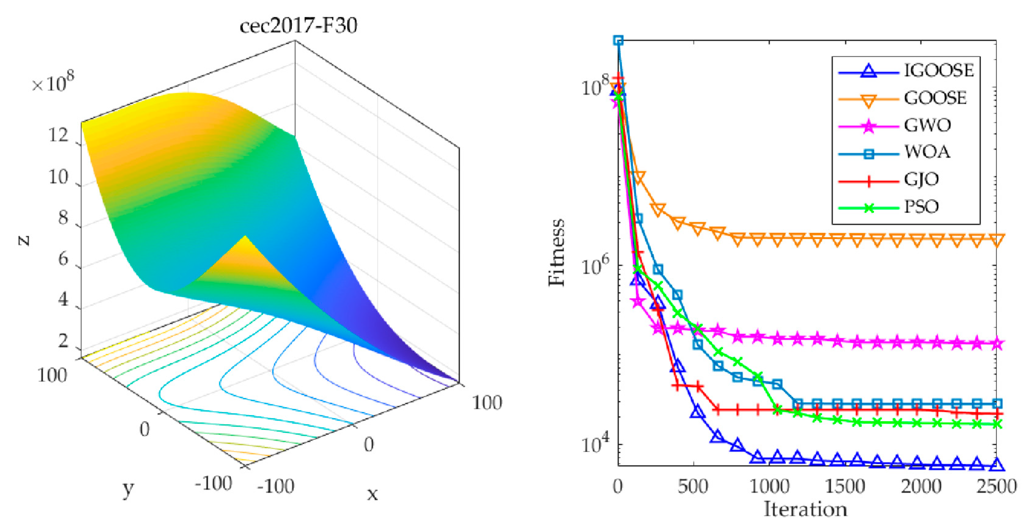
To evaluate the optimization performance of the IGOOSE, this study designed comparative experiments by subjecting the IGOOSE, alongside the GOOSE, the emerging Grey Wolf Optimizer (GWO), Whale Optimization Algorithm (WOA), Golden Jackal Optimization (GJO), and the widely recognized Particle Swarm Optimization (PSO) [29,30,31,32], to optimization tests on three benchmark functions under the CEC2017 dataset. During the experiments, the parameter settings of each algorithm were meticulously configured following standard procedures and are detailed in

Table 1. Parameter Settings of the Algorithm.

Algorithm	Parameter Settings
GOOSE	alphamax = 2, alphamin = 0
GWO	amax = 2, amin = 0
WOA	b = 1
GJO	-
PSO	w = 0.8, c1 = c2 = 1.5

to ensure the objectivity of experimental results. By analyzing the convergence curves of these algorithms, this study not only quantified their performance in terms of convergence speed and accuracy but also delved into their strategies and effectiveness in exploring and exploiting the search space while avoiding local optima. As illustrated in Figure 5, Figure 6 and Figure 7, these charts visually present the fitness trends of each algorithm on the three complex test functions: F2, F11, and F30.

The experimental results indicate that the IGOOSE, with its unique optimization strategies, exhibits significant advantages in convergence speed, stability, and global search capability. In particular, its improved optimization mechanism effectively accelerates the convergence process and significantly reduces the final optimal fitness value, demonstrating the efficiency and accuracy of the algorithm in solving complex optimization problems. Furthermore, the IGOOSE demonstrates robust capabilities in escaping local optima, enabling it to effectively jump out of local extrema regions and comprehensively search the solution space for better global solutions.

To enhance the robustness of the experimental results, this study further conducted replication experiments under controlled experimental conditions, specifically setting the maximum number of iterations to 2500. Specifically, each algorithm was independently executed 30 times to eliminate the potential influence of randomness introduced by a single run. Based on this, the standard deviation (Std) and average value (Avg) of each experiment were calculated and recorded as quantitative indicators to evaluate the optimization performance of the algorithms, as detailed in

Table 2. Comparison of the results of several test functions run by CEC2017.

Function	Index	IGOOSE	GOOSE	GWO	WOA	GJO	PSO
F2	Std	8.047 × 10−5	8.157 × 10−5	1.004 × 107	1.484 × 104	8.916 × 107	5.519 × 107
	Ave	2.000 × 102	2.000 × 102	2.796 × 106	1.547 × 104	2.943 × 107	1.062 × 107
F11	Std	9.235	5.984 × 101	2.837 × 101	9.482 × 101	3.516 × 101	1.571 × 101
	Ave	1.115 × 103	1.204 × 103	1.131 × 103	1.207 × 103	1.140 × 103	1.115 × 103
F30	Std	4.618 × 105	9.171 × 105	7.455 × 105	5.471 × 105	7.915 × 105	1.717 × 106
	Ave	3.316 × 105	4.692 × 105	5.694 × 105	4.679 × 105	6.256 × 105	8.979 × 105

. Through a comprehensive examination and comparative analysis of the data, it can be clearly observed that the IGOOSE exhibits relatively superior performance in both the standard deviation and average value dimensions compared to other optimization algorithms under comparison. Specifically, its lower standard deviation reflects the stability and reliability of the algorithm’s results, while the relatively lower average value demonstrates the advantages of the IGOOSE in terms of solution efficiency and accuracy.

4.2. Simulation Verification

To ensure the uniqueness of our validation approach, this study employs synthetic signals tailored specifically to mimic the characteristics of rolling bearing vibrations. The formulation for these custom-generated signals is elaborated as follows:

$$s(t)=y_0{e}^{-2\pi f_n\xi t}\sin (2\pi f_n\sqrt{1-{\xi }^2}t)$$

(37)

In the aforementioned equation, we define a carrier frequency, f_n = 3000 Hz, and a damping factor, ξ = 0.1. The signal is sampled at a frequency f_s = 20,000 Hz, with t representing individual sampling instants within a period T = 0.01 s. The total number of samples acquired is N = 4096, and the characteristic failure frequency under investigation is denoted as f₀ = 100 Hz.

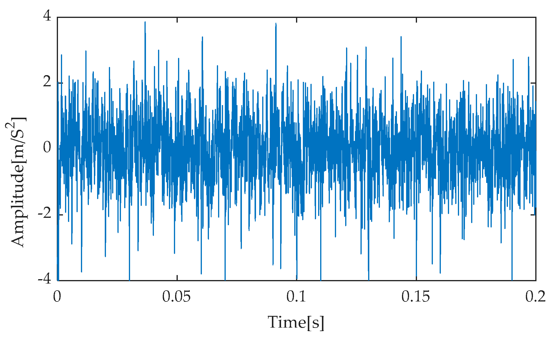
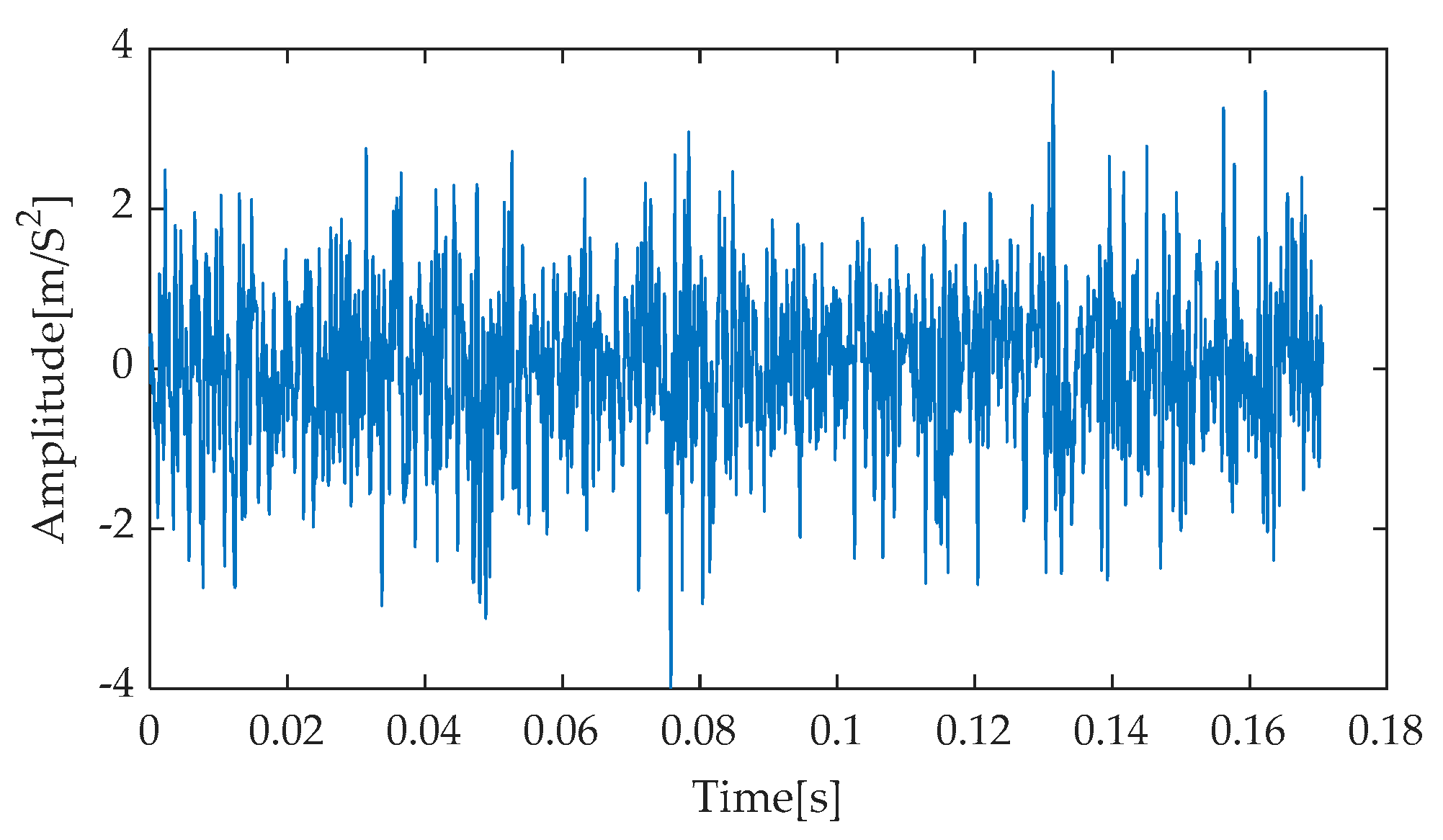
In this experiment, to simulate potential bearing faults in real-world scenarios, noise with a signal-to-noise ratio (SNR) of −7 dB was introduced into the simulated signal. This step aimed to mimic signal interference caused by environmental factors or inherent equipment issues under actual operating conditions. The simulation and analysis were conducted using the MATLAB R2023b software platform, with the objective of observing and analyzing signal characteristics against a strong noise background. 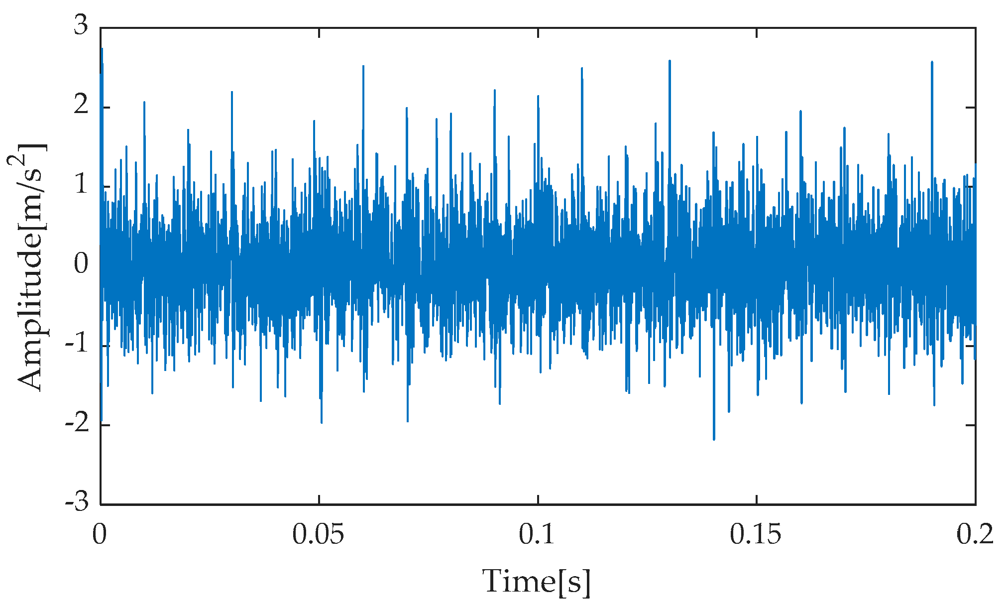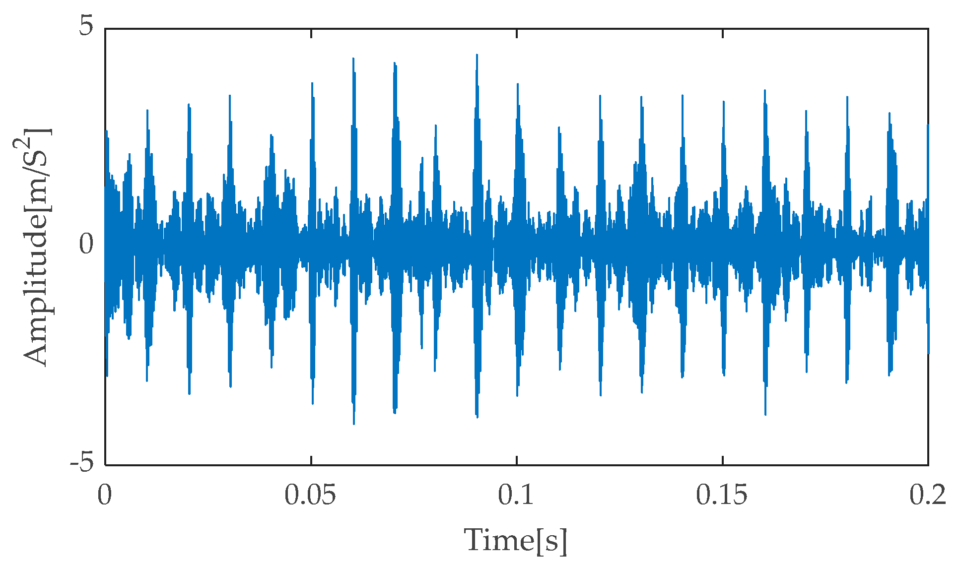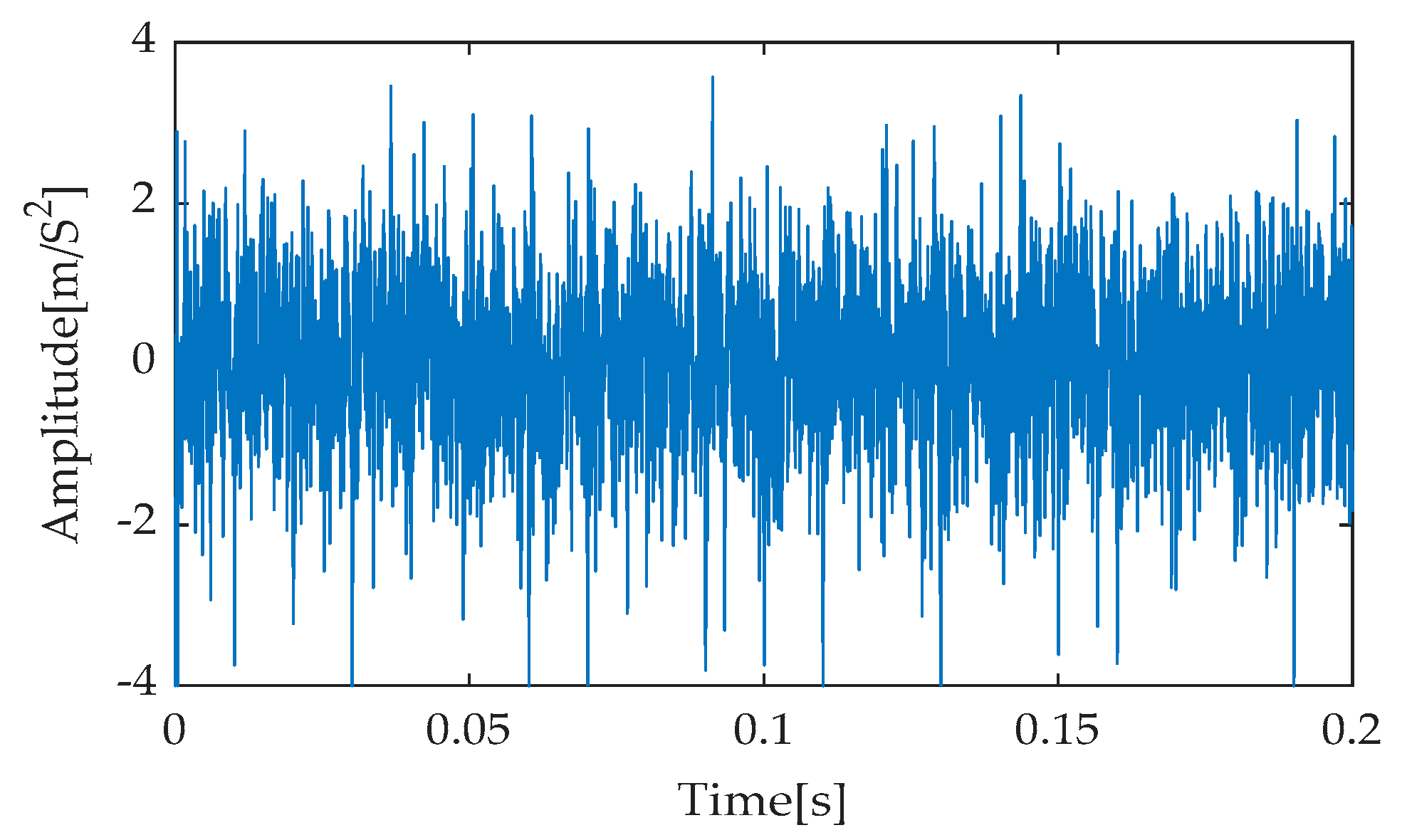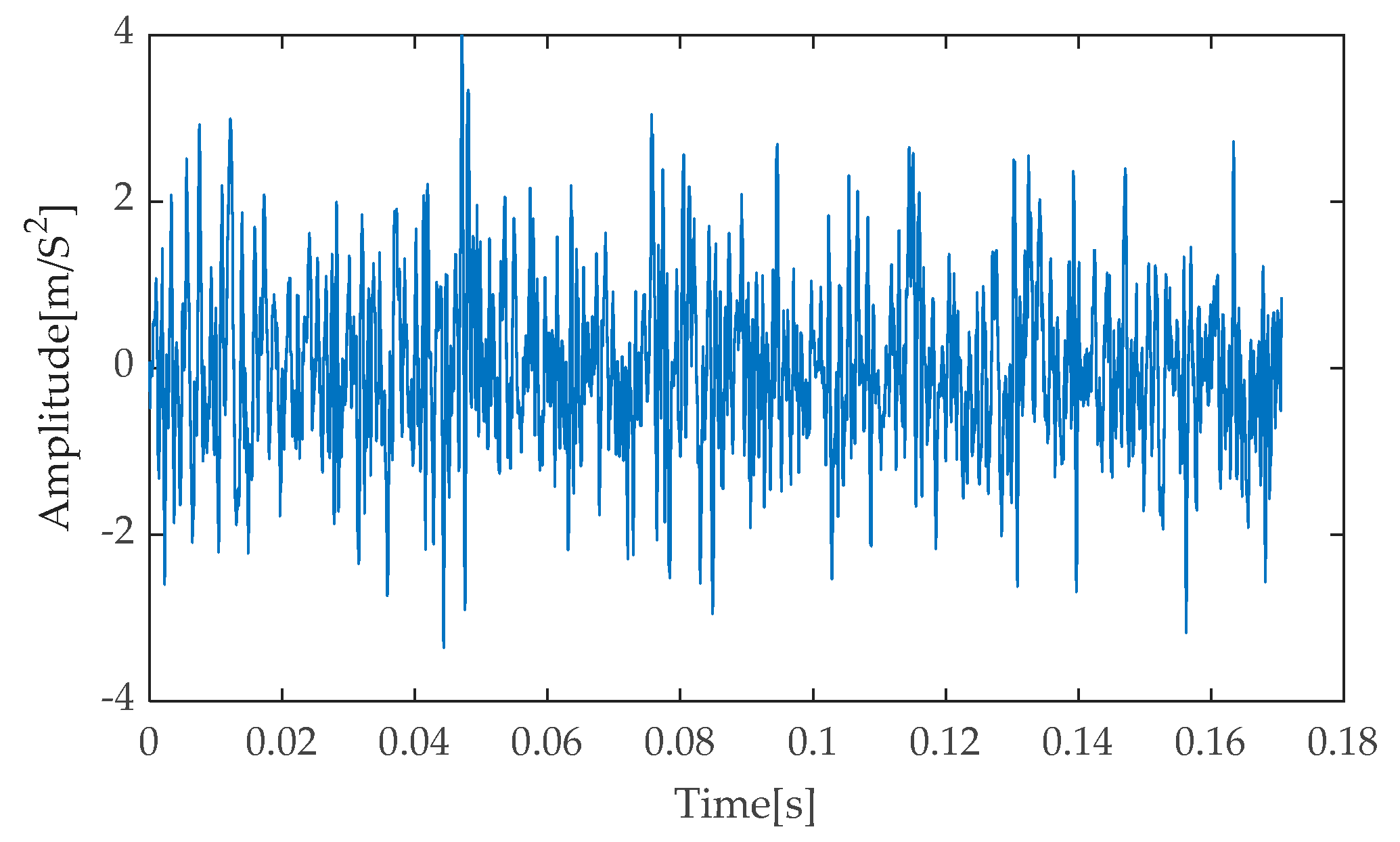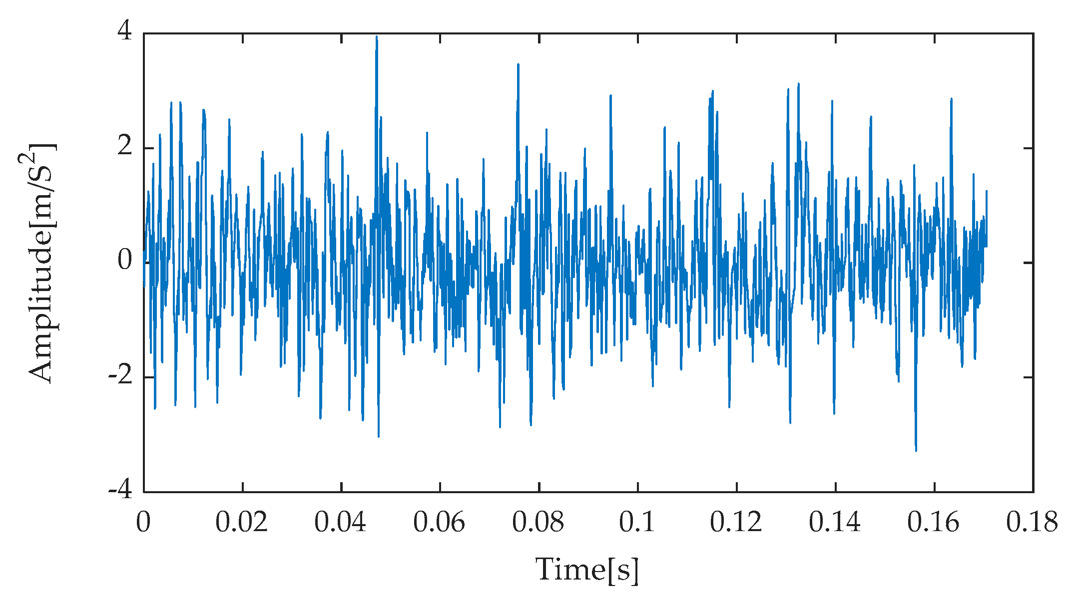Figure 8 presents the time–domain waveform of the original, noise-free simulated signal, serving as a benchmark for comparison with subsequent processing results. Subsequently, after incorporating noise with an SNR of −7 dB into the simulated signal, the resulting noisy simulated signal’s time–domain waveform is depicted in Figure 9. As evident from Figure 9, the strong background noise significantly overwhelms the periodic features originally present in the simulated signal, rendering it extremely challenging to directly extract useful fault information from the time–domain waveform. Consequently, further processing and analysis of the noisy signal are necessary.

Given the significant interference posed by noise on signals, this study introduces an IGOOSE strategy to optimize the critical parameters of VMD, specifically the selection of the number of modal components K and the penalty factor a. This optimization process aims to lay a solid foundation for subsequent signal decomposition by precisely configuring the initialization parameters of VMD. In implementing the IGOOSE algorithm, an Energy-Based Evaluation Criterion Index (E_ECI) proposed in this paper is designed and adopted as the fitness function to automatically search and optimize the VMD parameters, ensuring optimal decomposition results. During the initialization phase of IGOOSE, meticulous optimization operations are focused on the two crucial parameters in VMD: the number of modal components and the penalty factor. Specifically, the search range for the number of decomposition components is set to [2, 10], while the penalty factor is searched within the interval [100, 5000], ensuring that the algorithm explores within a reasonable parameter space. Additionally, in IGOOSE, a population size of 30 and a maximum number of iterations of 30 are configured to promote stable convergence and efficient execution of the algorithm.

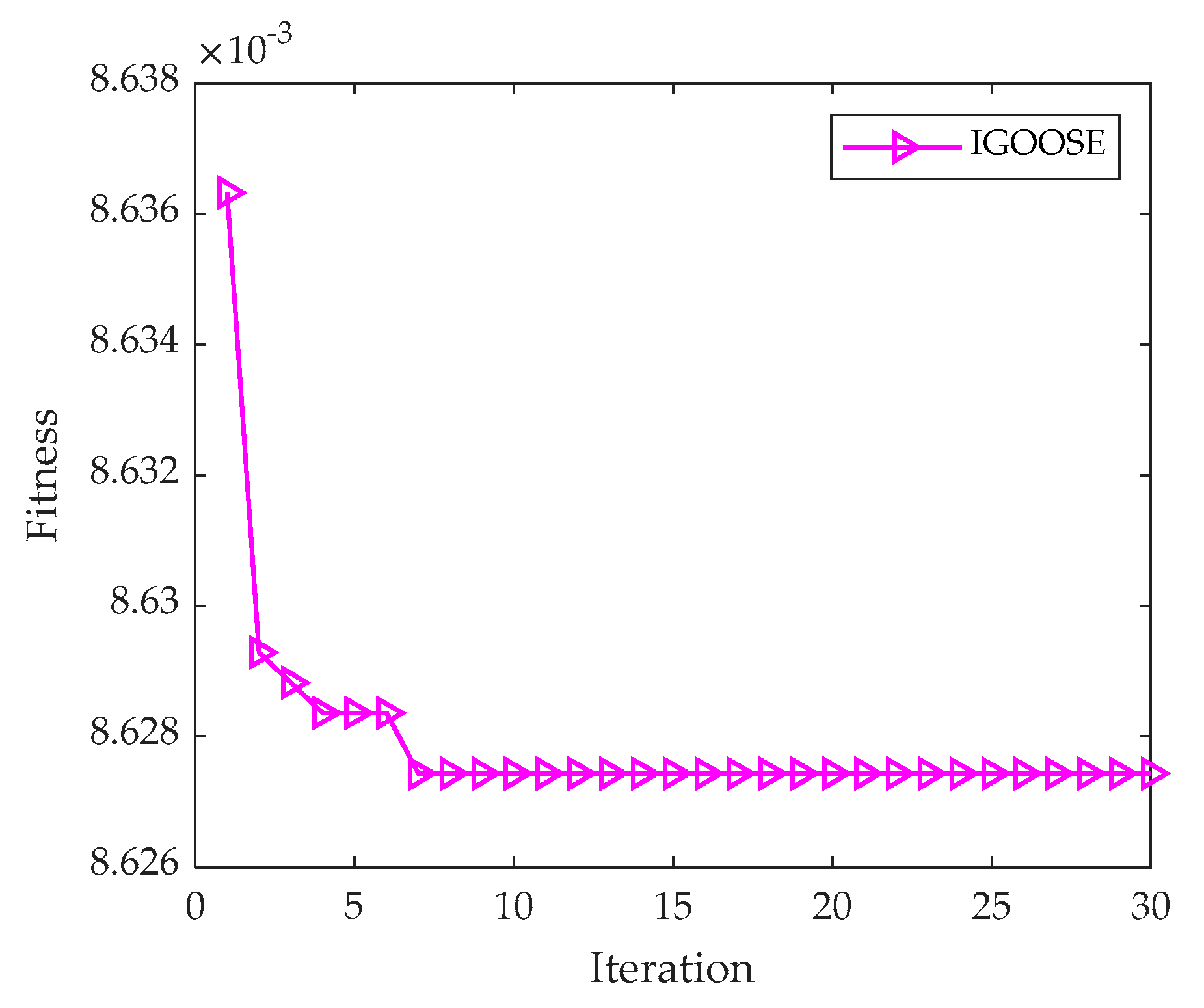
As depicted in Figure 10, the fitness curve variation of IGOOSE visually illustrates the rapid convergence of the algorithm to the optimal solution. Upon reaching the optimal fitness value, the experiment determines the optimal number of decomposition components to be 2 and the optimal penalty factor to be 4237. These optimized parameters are then applied to the VMD model for effective decomposition of the noisy simulated signal. To comprehensively evaluate the effectiveness of the IGOOSE-VMD method, this study also conducted parallel comparative experiments using Empirical Mode Decomposition (EMD), Ensemble Empirical Mode Decomposition (EEMD), Local Mean Decomposition (LMD), and Intrinsic Time-Scale Decomposition (ITD). Figure 11, Figure 12, Figure 13, Figure 14 and Figure 15 showcase the signal decomposition results obtained using IGOOSE-VMD, EMD, LMD, EEMD, and ITD, respectively, providing intuitive visual references for subsequent performance comparisons and in-depth analysis.

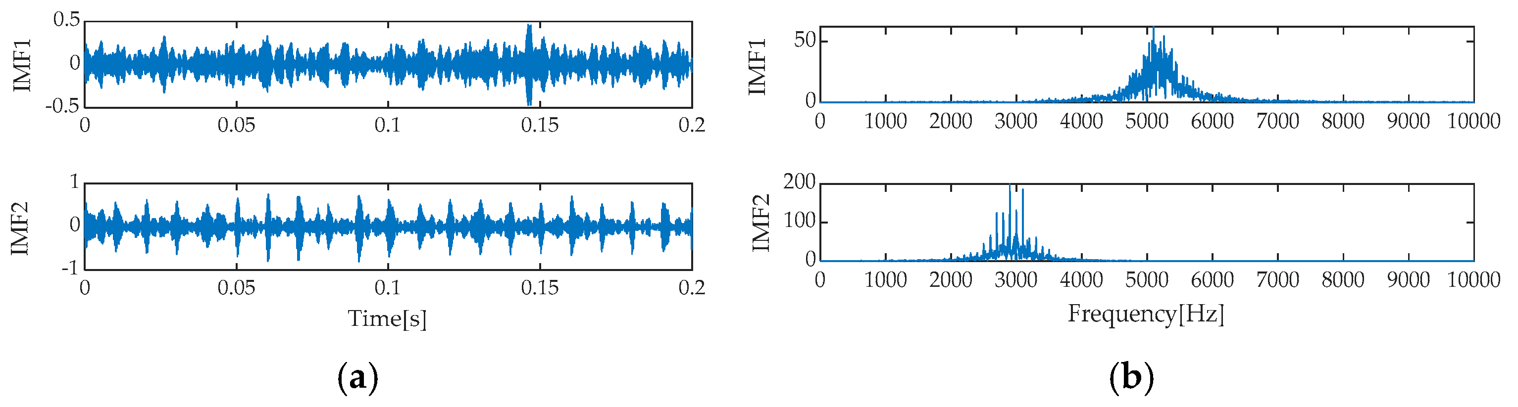
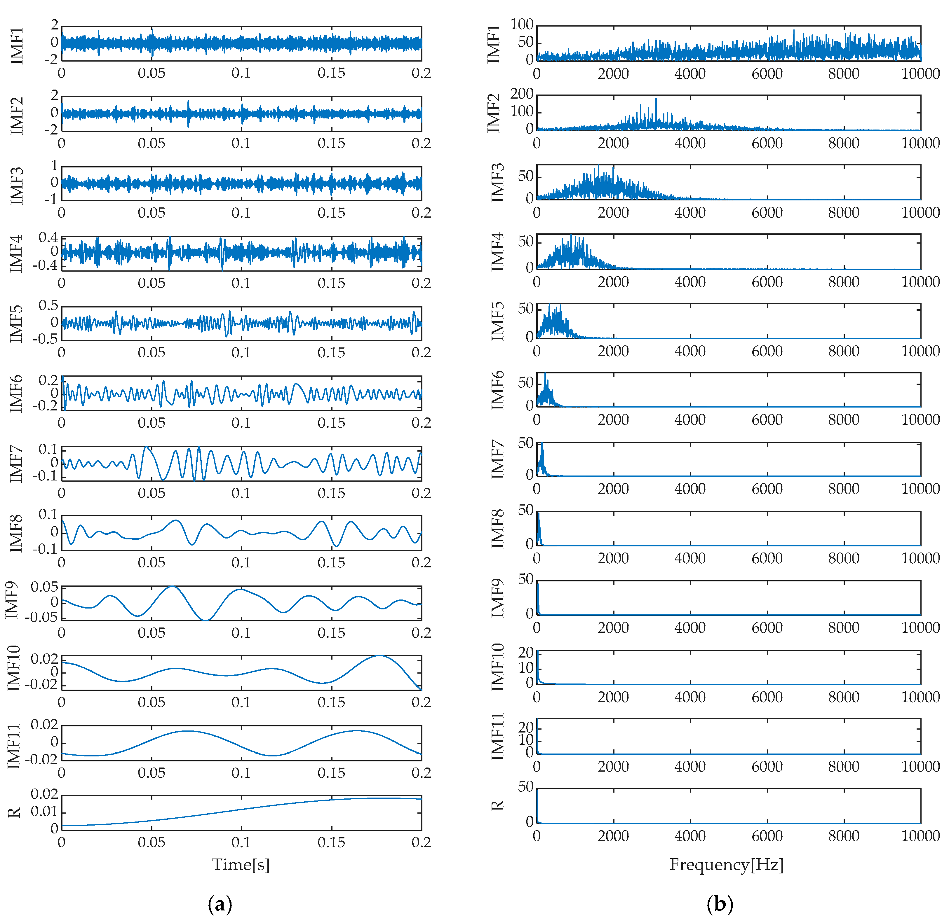
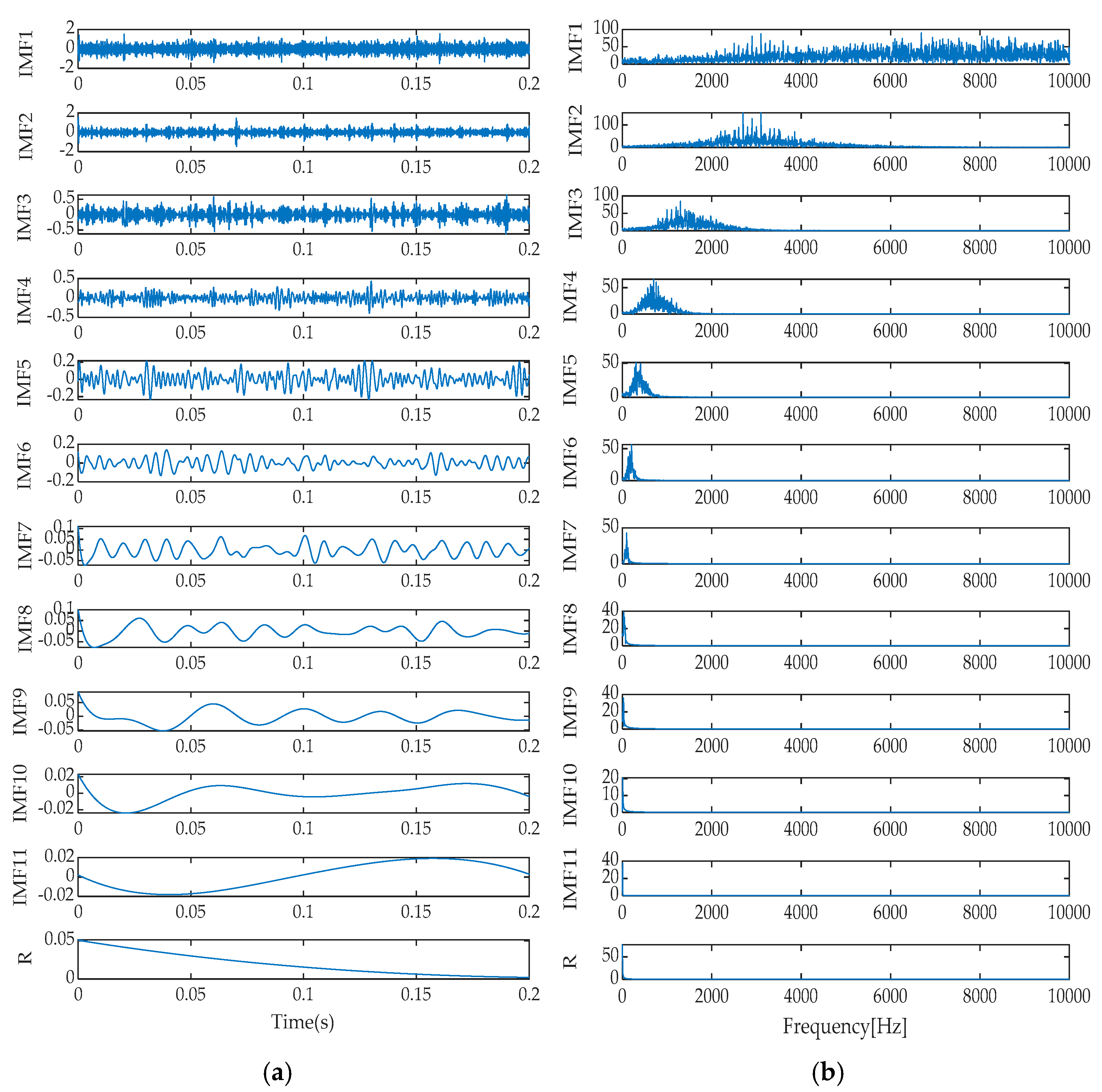
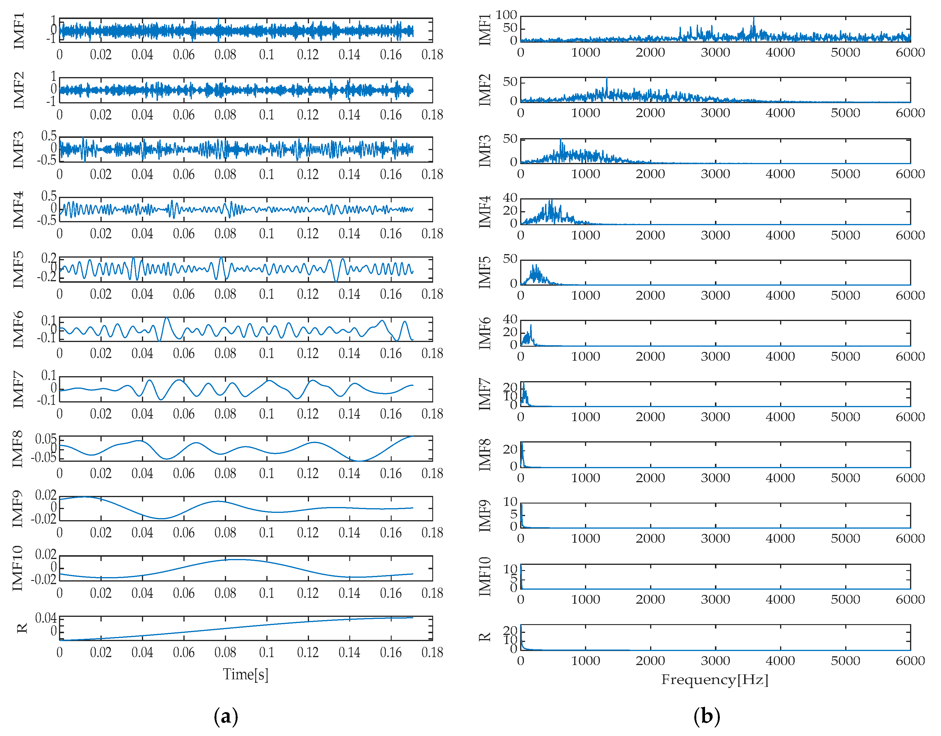
Upon a thorough analysis of the decomposition effects presented in Figure 11, Figure 12, Figure 13, Figure 14 and Figure 15, we can clearly observe the differences in performance among various signal decomposition methods. Specifically, after processing the signal using the IGOOSE-VMD method, two signal components were successfully separated, with their spectral characteristics exhibiting excellent separation and no overlap, ensuring uniformity and clarity in the spectral distribution. In contrast, the EMD method yielded 11 signal components and 1 residual component. Its time–domain representation distinctly identifies the presence of mode mixing, which is further corroborated in the frequency spectrum, particularly between IMF1, IMF2, and IMF3 components, where significant spectral overlap affects the purity and effectiveness of signal decomposition. Moving on to the EEMD method, although designed to alleviate the mode mixing issue of EMD, in this experiment, it also produced 11 signal components and 1 residual component, with similar mode mixing phenomena visible in the time–domain plot as EMD, failing to significantly improve the signal decomposition outcome.

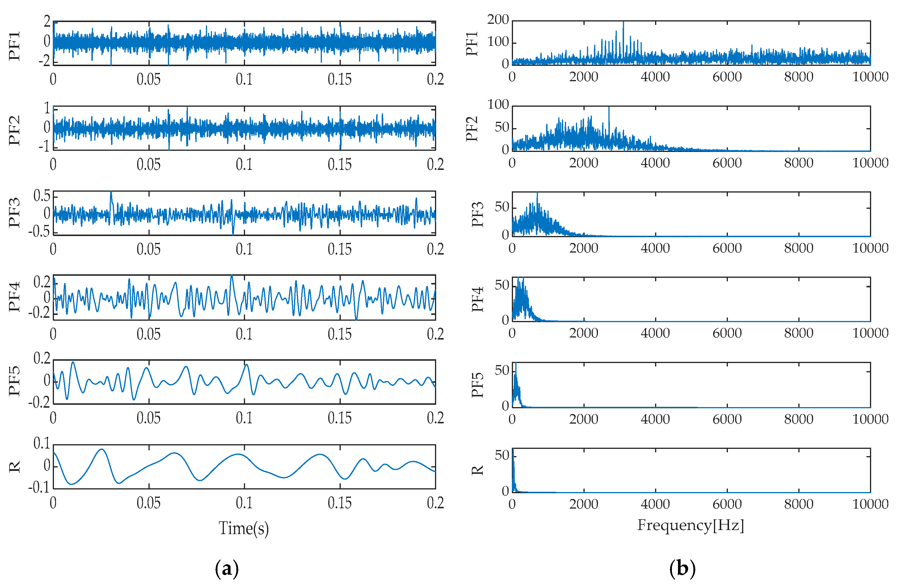
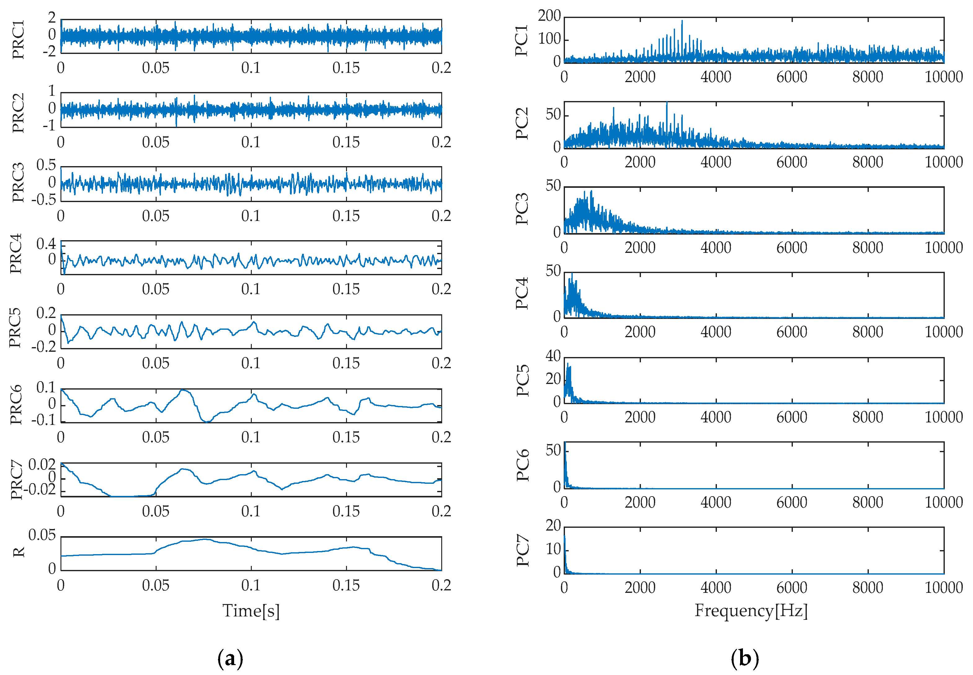
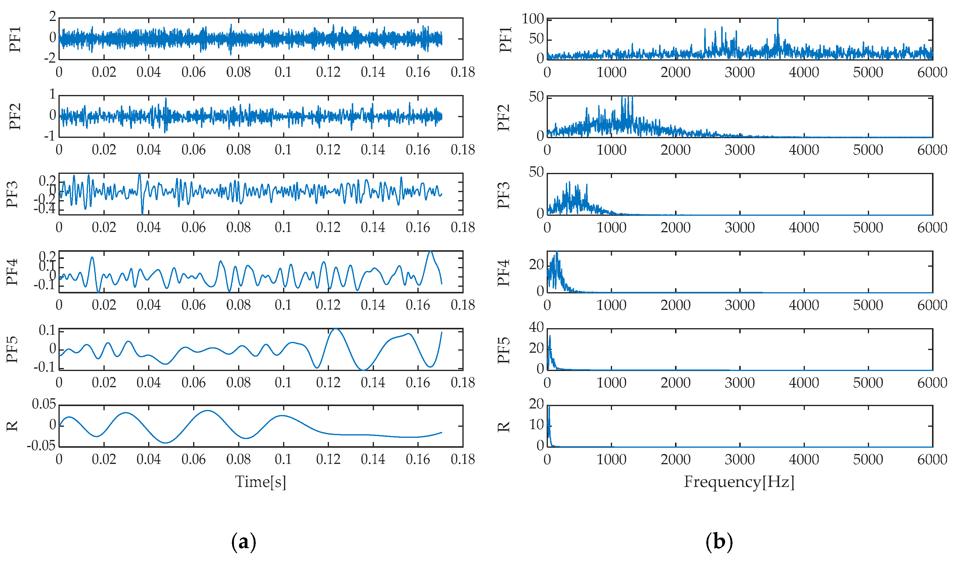
Additionally, the frequency spectra of the individual signal components exhibited spectral overlap, indicating that EEMD’s improvement is limited in handling complex, noisy signals. As for the LMD method, it decomposed the signal into five signal components and one residual component. Modal mixing was effectively suppressed in the time–domain plot. However, a certain degree of spectral overlap still existed between PF1 and PF3 components in the frequency spectrum, suggesting that while maintaining signal independence, further optimization of LMD’s spectral separation capability is needed. Finally, the ITD method decomposed the signal into seven signal components and one residual component, with signs of mode mixing reappearing in its time–domain representation. Meanwhile, notable spectral overlap between PRC1 and PRC3 components in the frequency spectrum indicates that ITD also faces challenges in mode separation and spectral clarity when dealing with complex signals. In summary, different signal decomposition methods exhibit their respective advantages and limitations when processing the same signal. Among them, IGOOSE-VMD performs relatively better in spectral separation.

To precisely select the most suitable signal components from the decomposition results of various signal time–frequency analysis methods, this study introduces the proposed E_ECI as the core evaluation criterion. Firstly, the E_ECI values of each signal component under each method were meticulously calculated and tabulated in

Table 3. Indicator result value (IGOOSE-VMD).

	IMF1	IMF2
EECI	0.001	0.018

,

Table 4. Indicator result value (EMD).

	IMF1	IMF2	IMF3	IMF4	IMF5	IMF6	IMF7	IMF8	IMF9	IMF10	IMF11
EECI	0.022	0.004	0.006	0.009	0.038	0.015	0.049	0.223	0.486	0.029	0.041

,

Table 5. Indicator result value (EEMD).

	IMF1	IMF2	IMF3	IMF4	IMF5	IMF6	IMF7	IMF8	IMF9	IMF10	IMF11
EECI	0.014	0.004	0.008	0.013	0.010	0.050	0.030	0.031	0.029	0.029	0.032

,

Table 6. Indicator result value (LMD).

	PF1	PF2	PF3	PF4	PF5
EECI	0.007	0.011	0.013	0.011	0.024

and

Table 7. Indicator result value (ITD).

	PRC1	PRC2	PRC3	PRC4	PRC5	PRC6	PRC7
EECI	0.008	0.010	0.020	0.025	0.088	0.018	0.022

for analysis. As evident from Table 3, the IMF1 component obtained from the IGOOSE-VMD method possesses the smallest E_ECI value, significantly indicating that the energy of the signal damage characteristic frequency is highly concentrated in this component, making the damage feature particularly prominent. Therefore, IMF1 was chosen for reconstructing the observed signal channel, while the remaining components were allocated to the reconstruction of the noise signal channel. Similarly, Table 4 reveals that after EMD decomposition, IMF2 exhibits the smallest E_ECI value, implying its excellence in capturing signal damage characteristics with energy concentrated at the damage characteristic frequency. Consequently, IMF2 was selected as the basis for reconstructing the observed signal channel, and the rest of the components were utilized for the noise channel reconstruction. Further analysis of Table 5 shows that the EEMD method also highlights the superiority of IMF2 in terms of E_ECI, further confirming its effectiveness in representing signal damage characteristics. Thus, IMF2 was designated as the core for reconstructing the observed signal channel, while the other components aided in constructing the noise signal channel.

In Table 6, the application of the LMD method indicates that PF1 has the smallest EECI value, demonstrating its high focus of energy distribution on the signal damage characteristic frequency, resulting in clear damage features. Hence, PF1 was utilized for reconstructing the observed signal channel, while the other components contributed to the reconstruction of the noise signal channel. Lastly, from Table 7, it is evident that the PRC1 component obtained from the ITD method possesses the smallest E_ECI value, which also proves the high concentration of energy on the signal damage characteristic in this component. Therefore, PRC1 was chosen as the key component for reconstructing the observed signal channel, and the remaining components were used to build the noise signal channel. Based on the above screening, this study further employed the RobustICA algorithm to effectively separate the signal from noise. Specifically, the proposed method was compared with traditional methods such as EMD-RobustICA, EEMD-RobustICA, LMD-RobustICA, and ITD-RobustICA in terms of noise reduction effects (as shown in Figure 16, Figure 17, Figure 18, Figure 19 and Figure 20).

Figure 16, Figure 17, Figure 18, Figure 19 and Figure 20 present the time–domain waveforms obtained after applying different noise reduction methods. Upon careful analysis, it is evident that the proposed IGOOSE-VMD-RobustICA method significantly enhances the visibility and clarity of the periodic impulsive components in the signal post-denoising. In contrast, while traditional methods such as EMD-RobustICA, EEMD-RobustICA, LMD-RobustICA, and ITD-RobustICA can also observe impulsive components to some extent after noise reduction, these components are often obscured by larger irrelevant noise peaks, leading to less clear waveforms.

Following the RobustICA noise reduction process, to comprehensively and deeply quantify the noise reduction performance of each method, the experimental analysis selected three indicators: cross-correlation coefficient, kurtosis, and mean absolute error (MAE) for a comprehensive analysis. These indicators not only reflect the similarity between the denoised signal and the original signal but also embody the sharpness of the signal waveform and the overall impact of noise reduction processing on signal errors. Specifically,

Table 8. Analysis of evaluation indicators.

Evaluating Indicator	Correlation Coefficient	Kurtosis	MAE
IGOOSE-VMD	0.649	5.097	0.789
EMD	0.493	4.413	0.722
EEMD	0.415	4.800	0.816
LMD	0.400	4.044	0.827
ITD	0.375	4.289	0.821

details the specific values of each evaluation indicator after applying different noise reduction methods. Notably, the IGOOSE-VMD-RobustICA method demonstrates significant advantages in both cross-correlation coefficient and kurtosis. Its cross-correlation coefficient reaches 0.649, indicating a high degree of similarity between the denoised signal and the original signal. The kurtosis value of 5.097 further reveals the effective enhancement in the clarity and sharpness of the impulsive components in the signal. Although this method slightly lags behind the EMD-RobustICA method in terms of MAE, the difference is relatively small. Further observation of the evaluation results for other methods reveals that, regardless of EMD-RobustICA, EEMD-RobustICA, LMD-RobustICA, or ITD-RobustICA, their performance in cross-correlation coefficient and kurtosis falls short of the IGOOSE-VMD-RobustICA method. While these traditional methods can reduce noise to a certain extent, they exhibit notable deficiencies in preserving signal characteristics and enhancing signal clarity.

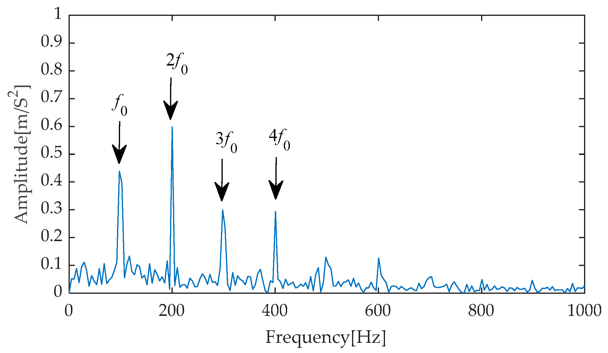
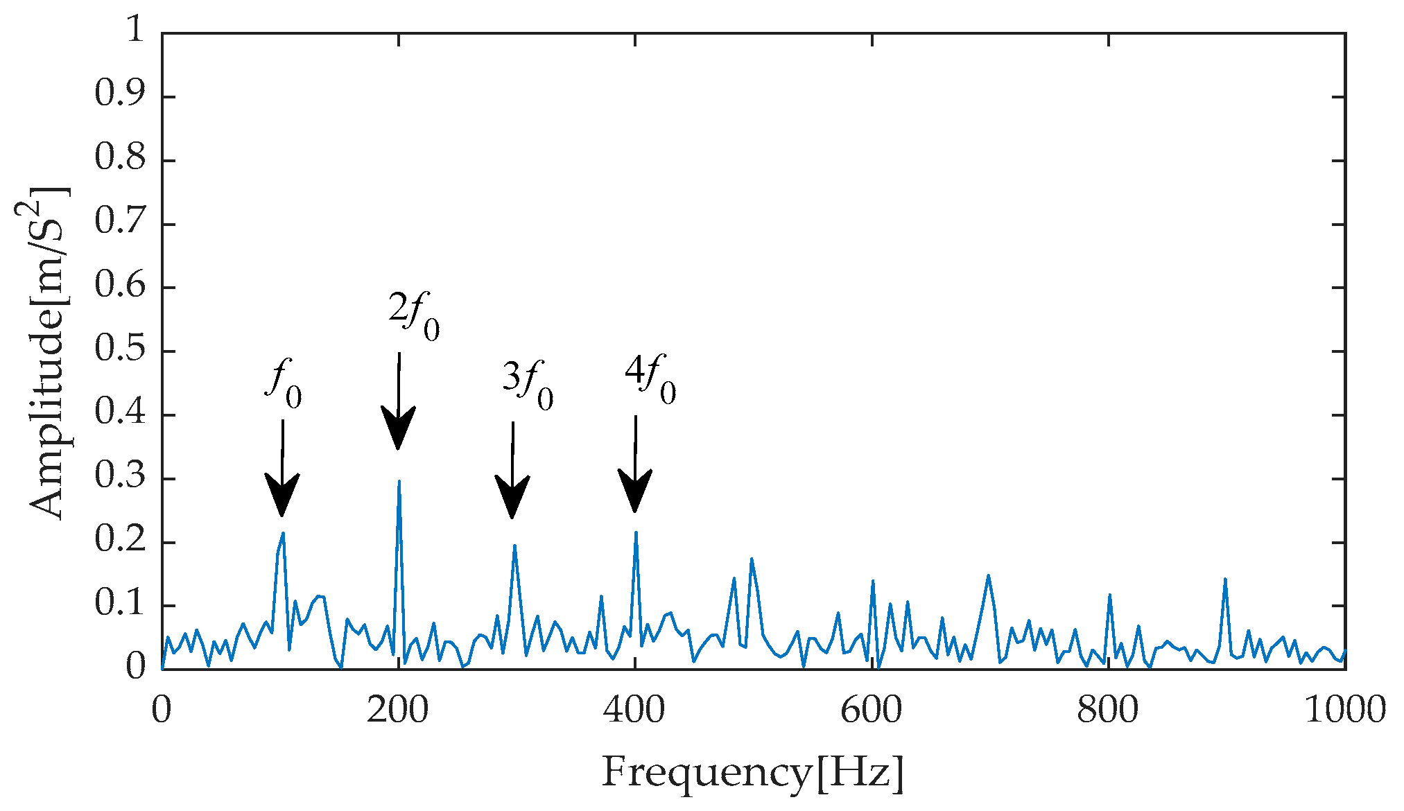
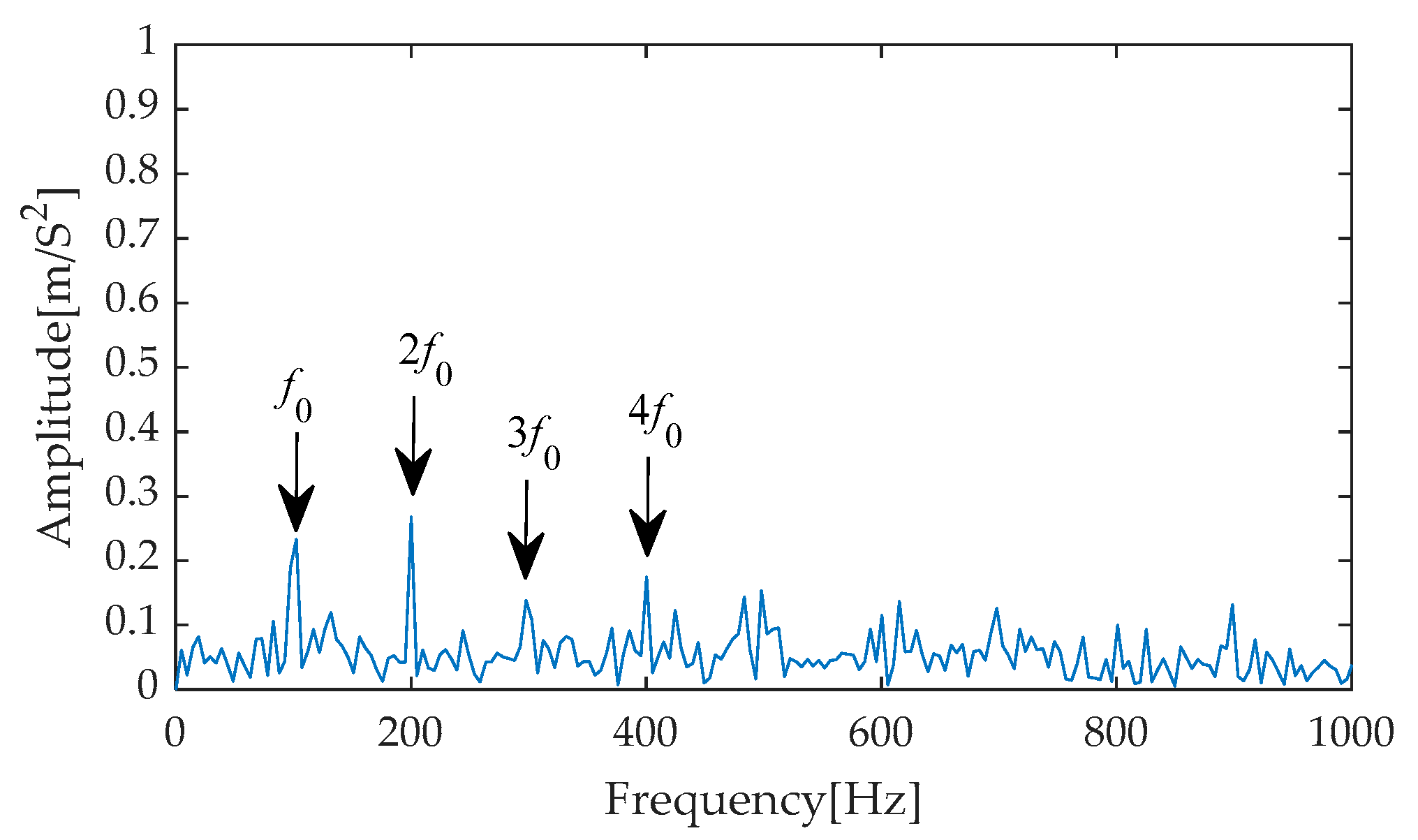
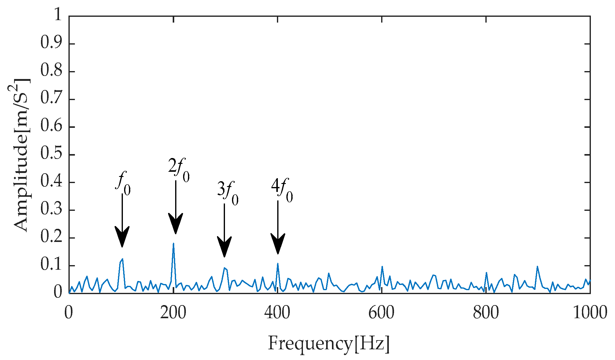
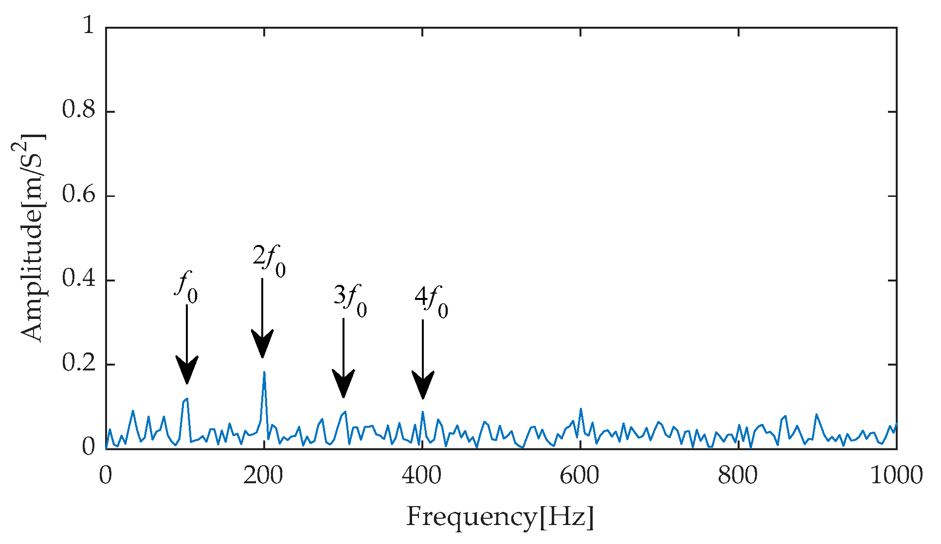
Furthermore, to precisely extract fault characteristics, Hilbert envelope demodulation was implemented on the results of effective signal-noise separation achieved through the aforementioned diverse methods. The resulting envelope spectra (as shown in Figure 21, Figure 22, Figure 23, Figure 24 and Figure 25) comprehensively display the frequency components under different processing methods, with notable changes particularly evident from the first to the fourth harmonics of the fault characteristics. Through comparative analysis, it can be observed that while methods such as EMD-RobustICA, EEMD-RobustICA, LMD-RobustICA, and ITD-RobustICA can reveal the existence of the first to the fourth harmonics of fault characteristics, the amplitudes of these frequency components are relatively low. Notably, in the envelope spectra of LMD-RobustICA and ITD-RobustICA, the amplitudes of fault frequencies are similar to those of background noise or irrelevant interference components, posing a significant challenge to the accuracy of fault diagnosis and increasing the risk of misdiagnosis or missed diagnoses.

In contrast, the envelope spectrum obtained using the IGOOSE-VMD-RobustICA method exhibits superior performance. Specifically, this method not only significantly enhances the amplitudes of the first to the fourth harmonics of fault characteristics, making them stand out among numerous frequency components and thereby more intuitively indicating the occurrence of faults, but also effectively reduces the interference from irrelevant components near the fault frequencies, greatly improving the clarity and accuracy of fault diagnosis. Subsequently, the signal denoised by the IGOOSE-VMD-RobustICA method is input into the CYCBD filter to further enhance the periodic impulsive characteristics in the signal.

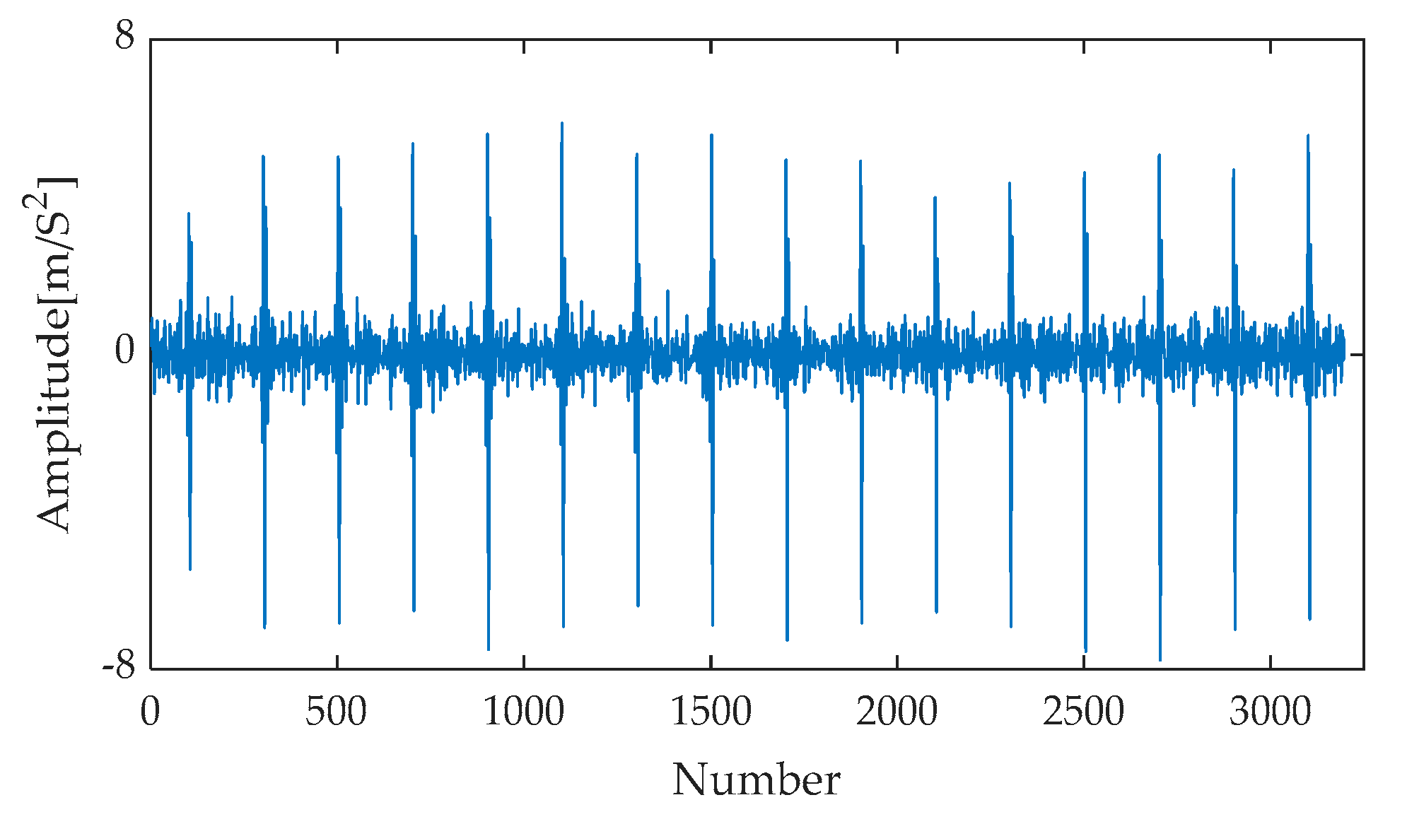
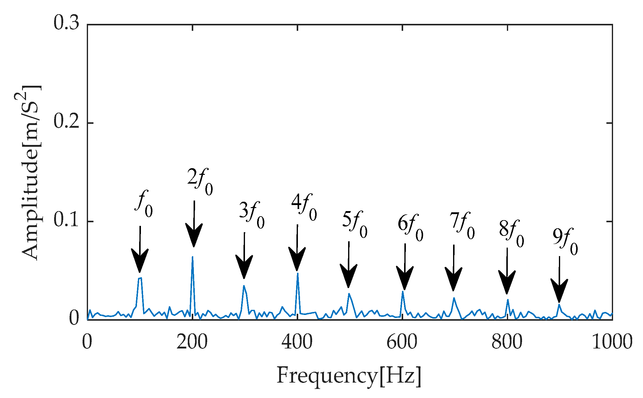
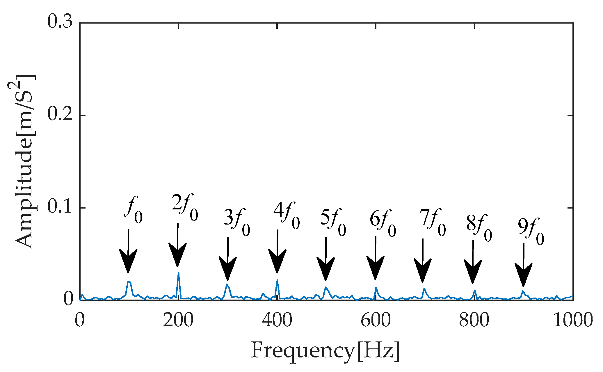
After the refinement of the original signal through the CYCBD filter, the experimental results yielded its time–domain waveform (as shown in Figure 26) and the corresponding envelope spectrum (as shown in Figure 27). In the time–domain waveform of Figure 26, the periodic impulse components within the signal are effectively extracted by the filter, becoming exceptionally clear with significantly enhanced amplitudes. Further observation of the envelope spectrum in Figure 27 reveals that within the crucial frequency range of 0 to 1000 Hz, the fault characteristic frequency and its second to ninth harmonics stand out prominently with extremely high amplitudes. This pronounced frequency distribution characteristic not only validates the effectiveness of the filter but also provides compelling evidence indicating the presence of a fault within the bearing system.

To comprehensively evaluate the effectiveness of different deconvolution methods in signal filtering, this study employed the signal denoised by the IGOOSE-VMD-RobustICA method and further processed it using three deconvolution techniques: Maximum Correlated Kurtosis Deconvolution (MCKD), Minimum Entropy Deconvolution (MED), and Optimal Minimum Entropy Deconvolution Adjusted (OMEDA) for in-depth filtering. To further analyze the filtering effects, the processed signals underwent Hilbert envelope analysis to generate envelope spectrums, with the results presented in Figure 28, Figure 29 and Figure 30. Upon careful examination of these envelope spectra, it becomes evident that the amplitudes of irrelevant interference components are significantly reduced after filtering with MCKD, MED, and OMEDA. Specifically, within the frequency range of 0 Hz to 1000 Hz, these methods can clearly identify and extract the fundamental frequency of the fault characteristic frequency along with its first to ninth harmonics, demonstrating their proficiency in complex signal analysis. However, it is noteworthy that despite the unique features and respective advantages of MCKD, MED, and OMEDA, when compared to the CYCBD method, they yield relatively lower amplitudes in extracting the fault characteristic frequencies. This further underscores the superiority of the CYCBD method in enhancing the amplitudes of fault characteristic frequencies.

4.3. Experimental Verification

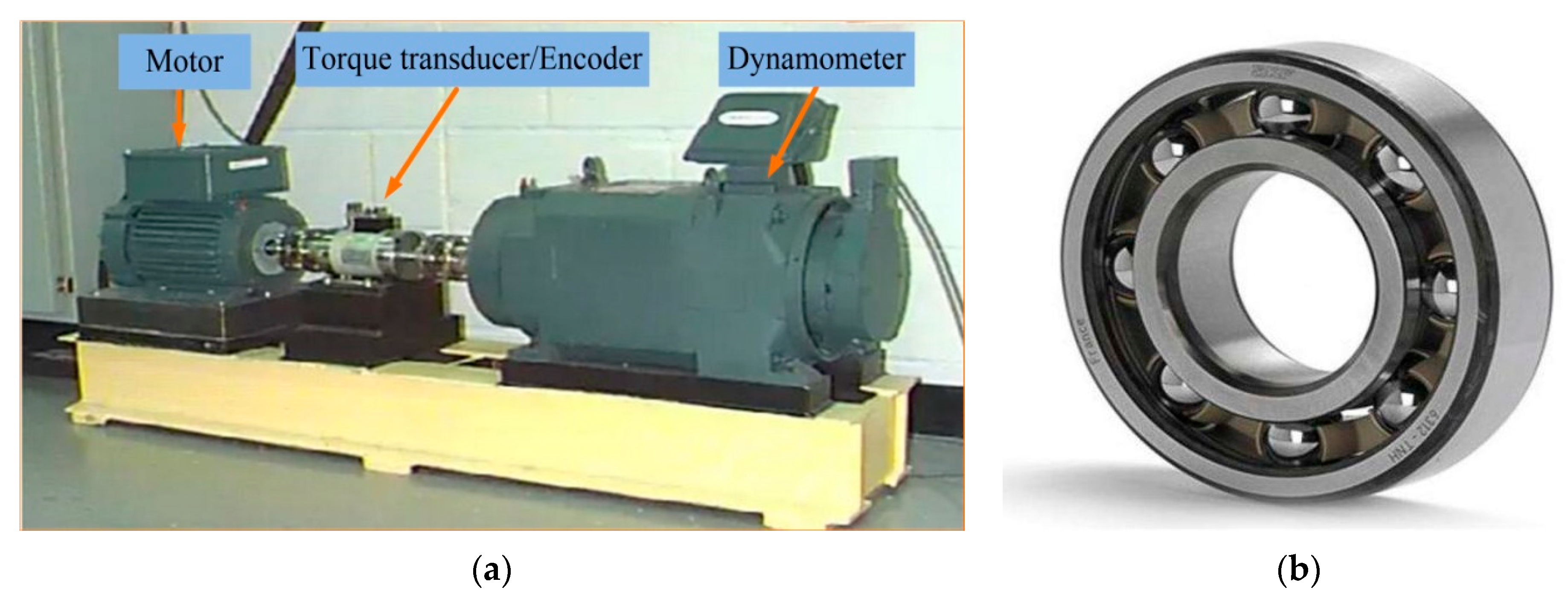
To validate the practical effectiveness of the proposed method, experiments were conducted using the publicly available bearing dataset from the renowned Case Western Reserve University for in-depth analysis. Figure 31 illustrates the overall architecture and components of the rolling bearing fault monitoring setup [33,34]. The core components of this experimental framework encompass the motor system, torque sensor devices, among others, which collaborate to establish a foundation of high precision and robustness for the experimental process. The experiments focused on a specific bearing model, namely the SKF6205 series, where single-point defects with a defined diameter were artificially introduced to critical locations of the bearings using advanced electrical discharge machining techniques, aiming to accurately simulate fault modes that may occur under actual operating conditions.

In terms of experimental parameter configuration, a sampling frequency of 12 kHz was meticulously selected as the standard for data acquisition, while the equipment was maintained at a constant rotational speed of 1797 revolutions per minute to ensure consistency and accuracy in data collection. Under these conditions, representative vibration signals were collected from the preset faults on the bearing inner race, with the intention of thoroughly analyzing the fault characteristics through these data.

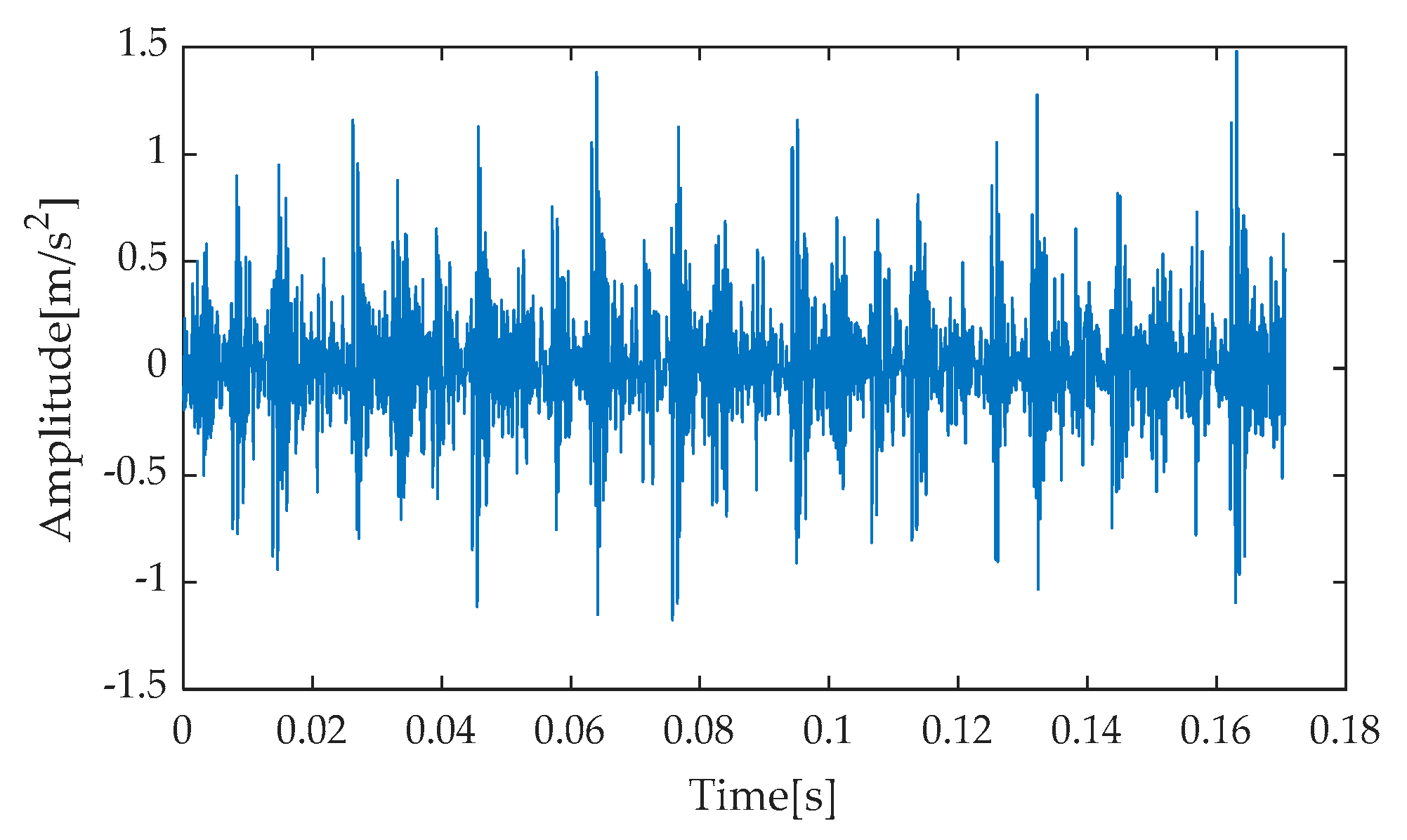
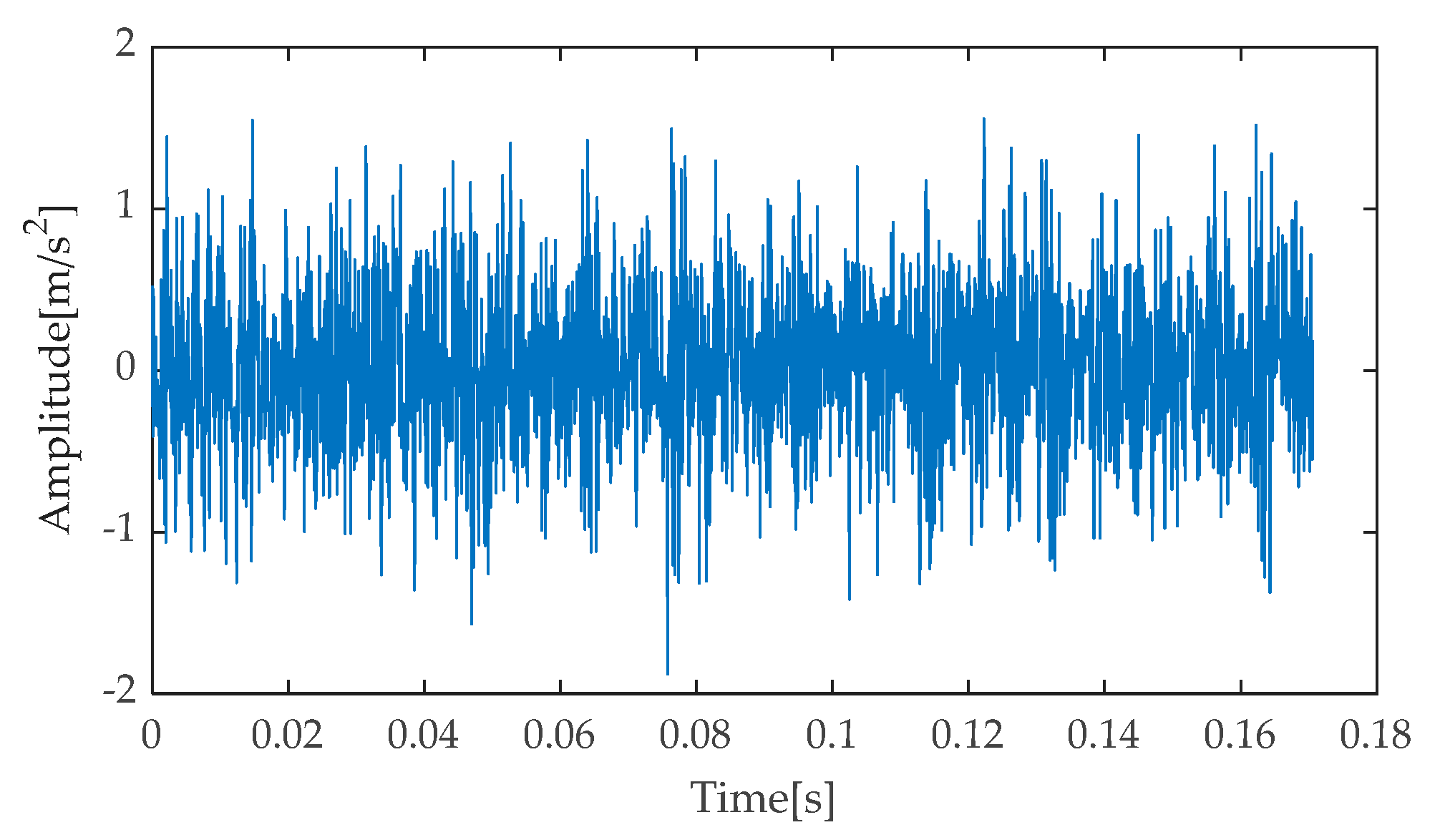
For the collected fault data, the time–domain waveform of the rolling bearing inner race fault is extracted, and the specific results are presented in Figure 32. Upon close examination of this waveform, it can be discerned that the noise interference is relatively weak. To further validate the practicality and robustness of the method proposed in this paper, noise with a signal-to-noise ratio (SNR) of −3 dB was introduced into the pure inner race fault signal, constructing a composite signal. The time–domain representation of this composite signal is shown in Figure 33. Observing Figure 33, it becomes evident that the introduction of noise significantly impacts the clarity of the original inner race fault signal, particularly making the distinctive impact features more subtle and difficult to identify against the noise background. This experimental design aims to simulate the complex signal environment under real operating conditions to comprehensively evaluate the performance of the proposed method.

Given the significant impact of noise interference in signal analysis, this study first optimizes the key parameters of VMD through the IGOOSE to fine-tune its core parameters—specifically, the number of decomposition components and the penalty factor. The goal is to strengthen the initial conditions of VMD through optimal parameter configuration, laying a solid foundation for subsequent signal analysis. In the implementation strategy of the IGOOSE, the E_ECI proposed in this paper is adopted as the fitness function to achieve automatic search and optimization of VMD parameters, ensuring the efficiency and precision of the decomposition process. During the initialization phase of the IGOOSE, the search ranges for the critical VMD parameters are experimentally set as follows: the search interval for the number of decomposition components is set to [2, 10], and the search space for the penalty factor is determined to be [100, 5000], ensuring that the algorithm can conduct a comprehensive exploration within a reasonable parameter domain. Furthermore, the population size is set to 30 individuals, and the maximum number of iterations is limited to 30, aiming to balance the convergence speed and computational efficiency of the algorithm.

Figure 34 illustrates the fitness evolution curve of the IGOOSE, clearly reflecting the dynamic process of the algorithm rapidly approaching and locking onto the optimal solution. Ultimately, the experiments determined the optimal number of decomposition components to be 7, and the optimal value of the penalty factor was set at 739. These optimized parameters were then input into the VMD model for high-quality decomposition of the noisy simulation signals. To comprehensively validate the superiority of the IGOOSE-VMD method, this study employed the same evaluation framework as in the simulation signal experiments and introduced comparative analysis methods such as EMD, EEMD, LMD, and ITD. Figure 35, Figure 36, Figure 37, Figure 38 and Figure 39 visually present the decomposition results of each method, providing rich data support for subsequent performance comparisons and in-depth analysis.

Upon meticulous analysis of the decomposition results presented in Figure 35, Figure 36, Figure 37, Figure 38 and Figure 39, we can clearly contrast the performance differences among various signal decomposition techniques. Specifically, when applying the IGOOSE-VMD method for signal decomposition, seven independent signal components were successfully extracted, exhibiting excellent separation performance in their spectral characteristics. The boundaries between spectra are distinct and free from overlap, ensuring the purity and clarity of spectral information. In contrast, the EMD method produced a combination of 10 signal components and 1 residual component. By observing its time–domain waveform, we can identify significant modal mixing, which is further confirmed in the corresponding frequency spectrum, particularly among IMF1, IMF2, and IMF3 components, where spectral overlap is particularly prominent.

As an improvement over EMD, the EEMD method aims to mitigate modal mixing. However, in our experiments, its output still included 10 signal components and 1 residual term, and the modal mixing issue in the time domain remained largely unresolved. Spectral overlap was also observed in the frequency spectrum, indicating that EEMD’s improvement is limited in decomposing signals under complex noise environments. The LMD method demonstrated different decomposition characteristics, yielding five signal components and one residual term. From a time–domain perspective, LMD effectively suppressed modal mixing, but at the spectral level, some degree of spectral overlap was still visible among PF1 to PF3 components. Finally, the ITD method decomposed the signal into seven signal components and one residual term. Modal mixing reappeared in its time–domain representation, and spectral overlap between PRC1 and PRC3 components was also evident in the frequency spectrum.

To accurately identify and extract the most suitable signal components among various time–frequency analysis techniques, this study also employs the proposed E_ECI as an assessment criterion. During the experiments, the E_ECI values of each signal component under each time–frequency decomposition method were systematically calculated, and the detailed data were organized in

Table 9. Indicator result value (IGOOSE-VMD).

	IMF1	IMF2	IMF3	IMF4	IMF5	IMF6	IMF7
EECI	0.034	0.032	0.031	0.009	0.010	0.037	0.043

,

Table 10. Indicator result value (EMD).

	IMF1	IMF2	IMF3	IMF4	IMF5	IMF6	IMF7	IMF8	IMF9	IMF10
EECI	0.014	0.015	0.037	0.065	0.168	0.239	0.659	0.082	0.078	8.308

,

Table 11. Indicator result value (EEMD).

	IMF1	IMF2	IMF3	IMF4	IMF5	IMF6	IMF7	IMF8	IMF9	IMF10
EECI	0.013	0.014	0.032	0.066	0.266	0.356	4.496	0.176	0.303	0.091

,

Table 12. Indicator result value (LMD).

	PF1	PF2	PF3	PF4	PF5
EECI	0.017	0.032	0.062	0.267	0.078

and

Table 13. Indicator result value (ITD).

	PRC1	PRC2	PRC3	PRC4	PRC5	PRC6
EECI	0.037	0.053	0.031	0.033	0.036	0.053

for further analysis. From the exhaustive data in Table 9, it can be intuitively inferred that the IMF4 component decomposed by the IGOOSE-VMD method exhibits the lowest E_ECI value, strongly suggesting that the energy of the signal damage characteristic frequency within this component is highly concentrated, and the damage characteristics are particularly prominent. Consequently, this study decides to adopt the IMF4 signal component as the basis for reconstructing the observation signal channel, while assigning the remaining components to the reconstruction system of the noise signal channel. Similarly, the data in Table 10 reveals the significant advantage of the IMF1 component decomposed by the EMD method in terms of E_ECI, indicating that its energy is efficiently concentrated at the damage characteristic frequency, demonstrating an exceptional ability to capture signal damage. Therefore, IMF1 is selected as the core for reconstructing the observation signal channel, while the remaining components contribute to the reconstruction of the noise channel. Upon further examination of Table 11, the EEMD method also highlights the leading position of the IMF1 component in E_ECI values. Therefore, IMF1 is chosen as the foundation for reconstructing the observation signal channel, with the remaining components aiding in the reconstruction of the noise signal channel. In the application analysis of the LMD method (as shown in Table 12), the PF1 component stands out with the lowest EECI value. Based on this, PF1 is designated as the primary component for reconstructing the observation signal channel, while the other components contribute to the construction of the noise signal channel. Finally, the data in Table 13 indicates that the PRC3 component decomposed by the ITD method possesses the smallest E_ECI value, which also verifies the high degree of energy concentration on the signal damage characteristic of this component. Therefore, PRC3 is identified as the crucial element for reconstructing the observation signal channel, and the remaining components are utilized in the construction of the noise signal channel. Based on these selection results, this study employs the same comparison criteria as in the simulation experiments to conduct an in-depth comparative analysis of the noise reduction performance between the proposed method and traditional methods such as EMD-RobustICA, EEMD-RobustICA, LMD-RobustICA, and ITD-RobustICA, aiming to comprehensively evaluate and validate the effectiveness of the proposed method.

During the thorough examination of the experimental results, Figure 40, Figure 41, Figure 42, Figure 43 and Figure 44 visually present the time–domain waveform characteristics after noise reduction using various methods. Through meticulous comparison and analysis of these waveforms, the IGOOSE-VMD-RobustICA method proposed in this paper demonstrates its unique superiority. Specifically, the processed signal exhibits a clearer waveform profile with prominently enhanced periodic impulse components, showcasing a high degree of clarity and discriminability. This characteristic is crucial for subsequent signal analysis and feature extraction. In contrast, traditional methods such as EMD-RobustICA, EEMD-RobustICA, LMD-RobustICA, and ITD-RobustICA, though capable of suppressing noise to some extent and revealing impulse components within the signal, are limited by higher background noise levels in the presentation of these components. Specifically, in the waveforms after noise reduction using these traditional methods, the impulse components are often surrounded or interfered with by more significant noise peaks that are not directly related to the signal characteristics, leading to a decrease in overall waveform clarity and affecting the accurate capture of the signal’s true characteristics.

In the subsequent stage of the experiment, we performed Hilbert envelope demodulation on the time–domain signals obtained after separating signals from noise through the aforementioned methods, aiming to precisely extract fault features. The resulting envelope spectra (Figure 45, Figure 46, Figure 47, Figure 48 and Figure 49) provided us with intuitive analytical evidence. Specifically, Figure 45 exhibits the envelope spectrum processed by the method proposed in this paper, where multiple prominent high-amplitude peaks are clearly visible, particularly the first and second harmonics of the fault characteristic frequency, which are distinctly outlined with prominent amplitudes. Notably, the amplitudes of unrelated interference components in the background remain at a low level, effectively reducing the disturbance to the identification of fault characteristics. In contrast, Figure 46, Figure 47, Figure 48 and Figure 49 present the envelope spectra obtained using traditional methods such as EMD-RobustICA, EEMD-RobustICA, LMD-RobustICA, and ITD-RobustICA, respectively. Although these methods can also capture the first and second harmonics of the fault characteristic frequency, their amplitudes appear relatively weaker and are surrounded by numerous unrelated interference waveforms with similar amplitudes, undoubtedly increasing the difficulty of fault feature identification and potentially leading to misinterpretation or omission in subsequent fault diagnosis. The aforementioned comparative analysis demonstrates that the method proposed in this paper exhibits superior performance in fault feature extraction, with more significant extraction effects, contributing to improved accuracy and reliability in fault diagnosis. To further enhance the periodic impulse characteristics in the signal, the denoised signal was input into the designed CYCBD filter, aiming to further highlight the crucial fault information within the signal.

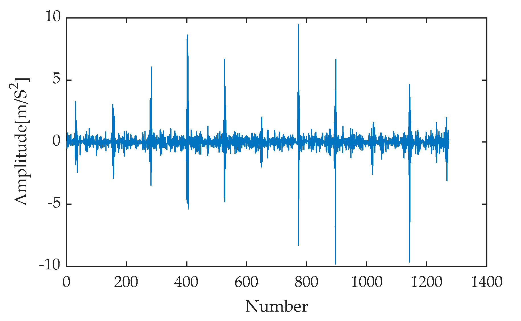
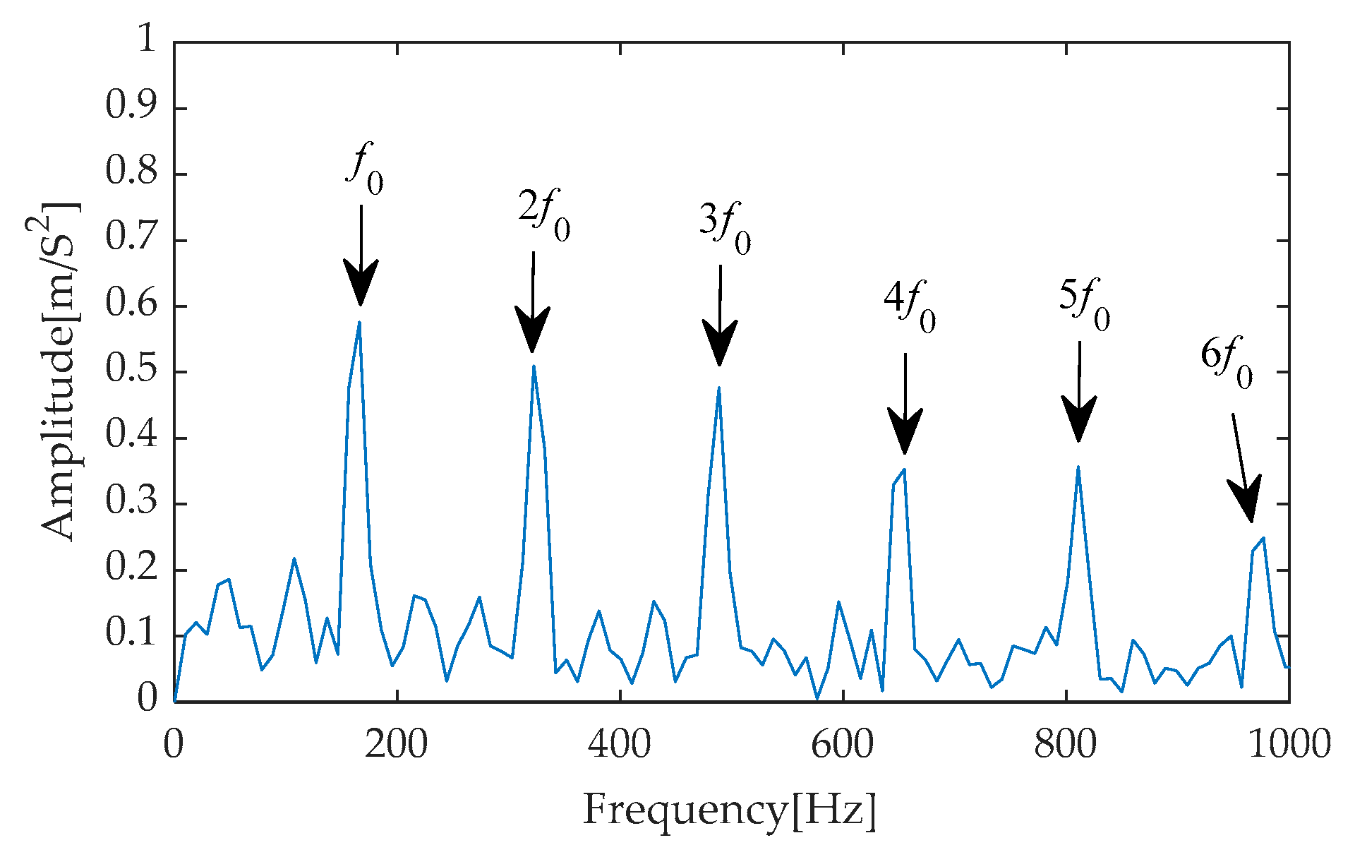
By inputting the signal processed by IGOOSE-VMD-RobustICA into the CYCBD filter for filtering, the experiment obtained an optimized time–domain waveform signal, as shown in Figure 50. In the depiction of the time–domain waveform in Figure 50, the filter successfully highlights the periodic impulse components within the signal, making them visually prominent and significantly amplifying their amplitudes, thereby demonstrating the effectiveness of the filtering process in enhancing signal characteristics. Subsequently, Hilbert envelope demodulation was performed on the filtered signal, and the corresponding envelope spectrum analysis is presented in Figure 51. The experiment focused on an in-depth analysis within the frequency range of 0 to 1000 Hz. Within this range, the fault characteristic frequency and its multiples (specifically, the second to sixth harmonics) are prominently displayed with extremely high amplitudes, forming a clearly distinguishable frequency distribution pattern. This phenomenon not only validates the excellent performance of the CYCBD filter in extracting and enhancing fault features but also strongly supports the conclusion that there is a fault in the inner race of the bearing system.

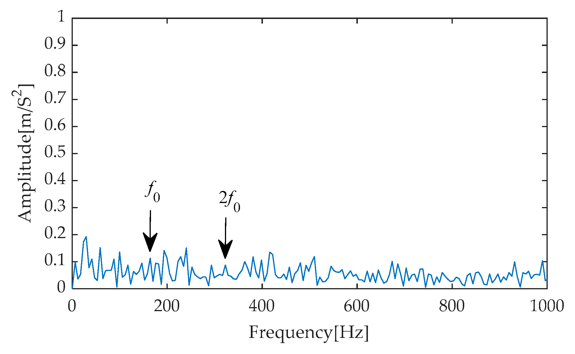
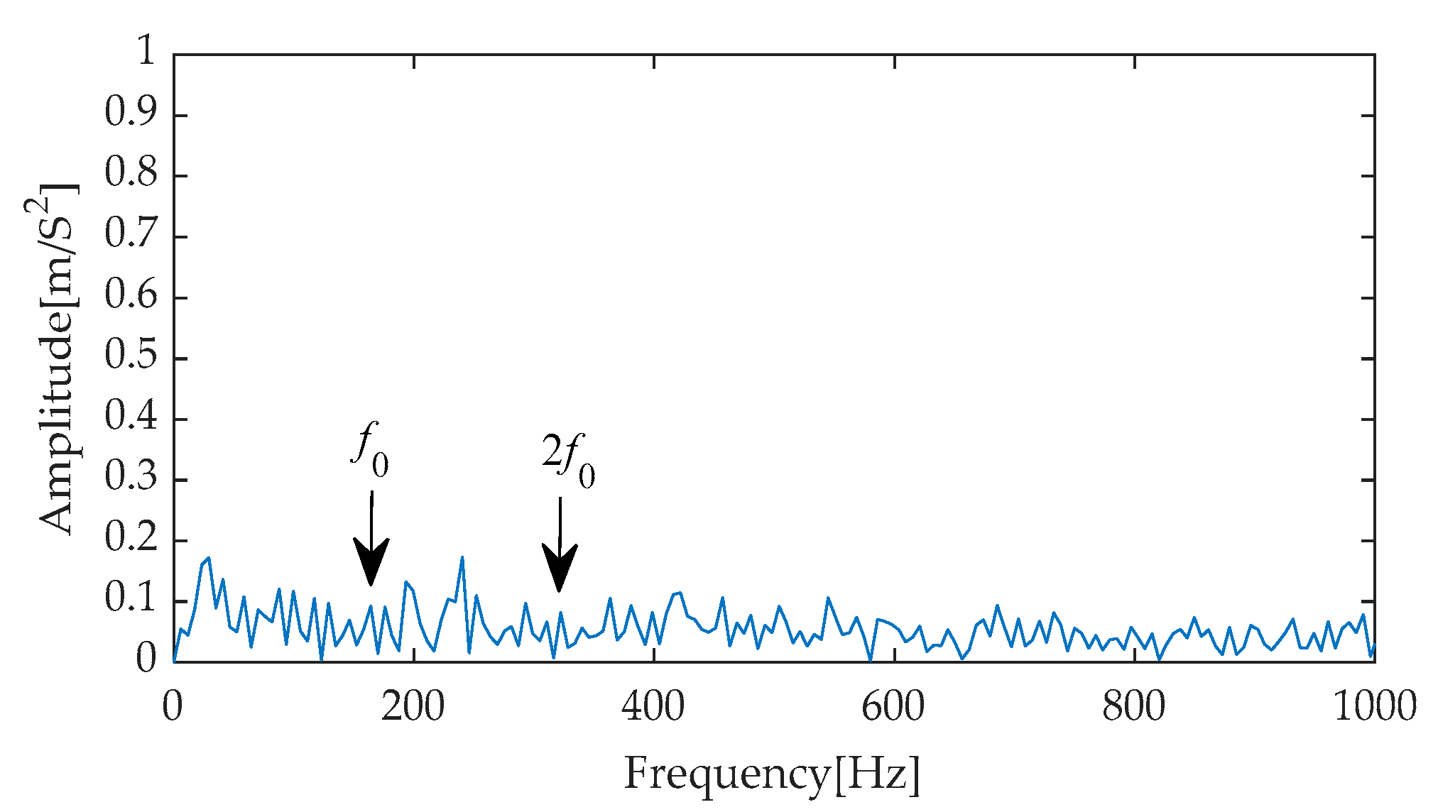
To comprehensively and laterally evaluate the filtering performance of the CYCBD method, this study further selected signals denoised by the IGOOSE-VMD-RobustICA algorithm as the analysis subjects. Subsequently, three deconvolution techniques, namely MCKD, MED, and OMEDA, were applied to these signals for in-depth filtering. To refine the assessment of filtering effects, Hilbert envelope analysis was conducted on the signals processed by each method, and corresponding envelope spectra were plotted, as shown in Figure 52, Figure 53 and Figure 54. Through meticulous analysis of these envelope spectra, it is observed that the MCKD, MED, and OMEDA methods are all capable of effectively extracting multiple harmonic components of the bearing inner race fault characteristic frequency. Specifically, within the frequency range of 0 Hz to 1000 Hz, the MCKD successfully identifies and extracts the first, second, and fifth harmonics of the inner race fault characteristic frequency; the MED similarly captures these harmonic components; whereas the OMEDA extends the detection range further, additionally extracting the third harmonic. These findings demonstrate the efficacy of these deconvolution techniques in fault feature extraction. However, compared to the CYCBD, while the aforementioned methods can identify similar fault characteristic frequencies, they exhibit relatively lower amplitudes in the extracted fault characteristic frequencies, and the envelope spectra still contain a certain degree of non-target component interference.

5. Conclusions

In the field of fault diagnosis for machinery rolling bearings, this study proposes a fault feature extraction method based on IGOOSE-optimized VMD technology combined with RobustICA-CYCBD. The following key conclusions are drawn:

(1)

Addressing the high parameter sensitivity of VMD when processing complex signals, this study introduces an improved GOOSE algorithm to optimize the initialization parameters of VMD. By incorporating refraction direction learning and mutation learning strategies into the IGOOSE, it better overcomes the limitations of GOOSE in balancing global and local optimization, enhancing the algorithm’s precision and speed in global optimization. Compared to optimization algorithms such as GOOSE, GWO, WOA, GJO, and PSO, the proposed algorithm demonstrates certain advantages in test functions.

(2)

During the optimization of VMD using the IGOOSE, an optimization strategy based on energy characteristic indicators is proposed, enabling automatic tuning of VMD’s initialization parameters. This method dynamically identifies and separates frequency bands closely related to the target fault mode, effectively avoiding modal aliasing and endpoint effects caused by inappropriate preset parameters, significantly improving the extraction accuracy of fault characteristic frequencies in nonstationary and nonlinear signals. Compared with traditional methods (e.g., EMD, EEMD, LMD, ITD), this study’s method exhibits stronger fault feature highlighting capabilities, providing robust support for accurately determining fault types.

(3)

This study designs a signal component selection mechanism based on energy characteristic indicators. By selecting the optimal signal component as input for the RobustICA observation channel, high-quality noise reduction of the signal is achieved. Experimental results show that, for both constructed simulation signals and actually collected rolling bearing signals, this method achieves better noise reduction performance compared to traditional combinations such as EMD-RobustICA, EEMD-RobustICA, LMD-RobustICA, and ITD-RobustICA. Moreover, the time–domain waveform of the denoised signal retains the characteristics of the original signal to a high degree, ensuring information integrity.

(4)

By applying CYCBD filtering to the signal after RobustICA noise reduction, this study successfully achieves deep enhancement and precise extraction of fault impact components. In both simulation experiments and tests based on the publicly available bearing dataset from Case Western Reserve University, this method accurately captures fault frequencies and their harmonic components. Compared to traditional methods based on EMD, EEMD, LMD, ITD, as well as filtering techniques like MCKD, MED, and OMEDA, it demonstrates superior fault feature extraction performance. This achievement not only enriches the technical means for rolling bearing fault diagnosis but also provides new insights into improving the accuracy and reliability of diagnosis.

The computational cost and real-time applicability of the fault feature extraction method proposed in this paper are worth discussing. In terms of computational cost, the iterative optimization of the IGOOSE algorithm and the VMD decomposition will increase the computational load. In subsequent research, further optimization of the algorithm will be conducted to reduce computational resource consumption. Meanwhile, given that the algorithm may still have shortcomings—such as suboptimal convergence speed and a tendency to be trapped in local optima—when dealing with complex signals, it is advisable to consider introducing more heuristic strategies or adaptive mechanisms in the future to further enhance the algorithm’s global search capability and convergence speed in order to meet the feature extraction requirements of rolling bearing fault signals under different operating conditions. Regarding real-time applicability, when faced with high-speed and continuous bearing fault monitoring, it is also necessary to further test the response speed and stability of this method under different data streams to ensure the timely and accurate extraction of fault features in real industrial scenarios, providing reliable support for real-time diagnosis of bearing faults.

References

1. Bracewell, R.N. The fourier transform. Sci. Am. 1989, 260, 86–95. [Google Scholar] [CrossRef] [PubMed]
2. Heckbert, P. Fourier transforms and the fast Fourier transform (FFT) algorithm. Comput. Graph. 1995, 2, 15–463. [Google Scholar]
3. Chen, J.Y.; Li, B.Z. The short-time Wigner–Ville distribution. Signal Process. 2024, 219, 109402. [Google Scholar] [CrossRef]
4. Huang, Z.; Chen, G.; Beer, M. Multi-taper S-transform method for estimating Wigner-Ville and Loève spectra of quasi-stationary harmonizable processes. Mech. Syst. Signal Process. 2024, 206, 110880. [Google Scholar] [CrossRef]
5. Dong, H.; Yu, G.; Lin, T.; Li, Y. An energy-concentrated wavelet transform for time-frequency analysis of transient signal. Signal Process. 2023, 206, 108934. [Google Scholar] [CrossRef]
6. Grobbelaar, M.; Phadikar, S.; Ghaderpour, E.; Struck, A.F.; Sinha, N.; Ghosh, R.; Ahmed, Z.I. A survey on denoising techniques of electroencephalogram signals using wavelet transform. Signals 2022, 3, 577–586. [Google Scholar] [CrossRef]
7. Pouyani, M.F.; Vali, M.; Ghasemi, M.A. Lung sound signal denoising using discrete wavelet transform and artificial neural network. Biomed. Signal Process. Control 2022, 72, 103329. [Google Scholar] [CrossRef]
8. Huang, N.E.; Shen, Z.; Long, S.R.; Wu, M.C.; Shih, H.H.; Zheng, Q.; Yen, N.-C.; Tung, C.C.; Liu, H.H. The Empirical Mode Decomposition and the Hilbert Spectrum for Nonlinear and Non-Stationary Time Series Analysis. Proc. R. Soc. Lond. A 1998, 454, 903–995. [Google Scholar] [CrossRef]
9. Zhang, J.; Sang, H.; Zhao, S. EMD-based time–frequency denoising algorithm for the self-sensing of vibration signals in ultrasonic-assisted grinding. Meas. Sci. Technol. 2022, 33, 104004. [Google Scholar] [CrossRef]
10. Wu, Z.; Huang, N.E. Ensemble Empirical Mode Decomposition: A Noise-Assisted Data Analysis Method. Adv. Adapt. Data Anal. 2009, 1, 1–41. [Google Scholar] [CrossRef]
11. Dao, F.; Zeng, Y.; Qian, J. A novel denoising method of the hydro-turbine runner for fault signal based on WT-EEMD. Measurement 2023, 219, 113306. [Google Scholar] [CrossRef]
12. Smith, J.S. The Local Mean Decomposition and Its Application to EEG Perception Data. J. R. Soc. Interface 2005, 2, 443–454. [Google Scholar] [CrossRef] [PubMed]
13. Zhao, H.; Li, X.; Liu, Z.; Wen, H.; He, J. A Double Interpolation and Mutation Interval Reconstruction LMD and Its Application in Fault Diagnosis of Reciprocating Compressor. Appl. Sci. 2023, 13, 7543. [Google Scholar] [CrossRef]
14. Frei, M.G.; Osorio, I. Intrinsic time-scale decomposition: Time-frequency energy analysis and real-time filtering of nonstationary signals. Proc. R. Soc. Lond. 2007, 463, 321–342. [Google Scholar] [CrossRef]
15. Gao, S.; Xu, L.; Li, Y.; Ji, J. Roll eccentricity extraction and compensation based on MPSO-WTD and ITD. PLoS ONE 2022, 17, e0259810. [Google Scholar] [CrossRef] [PubMed]
16. Dragomiretskiy, K.; Zosso, D. Variational mode decomposition. IEEE Trans. Signal Process. 2013, 62, 531–544. [Google Scholar] [CrossRef]
17. Jin, Z.; Chen, D.; He, D.; Sun, Y.; Yin, X. Bearing fault diagnosis based on VMD and improved CNN. J. Fail. Anal. Prev. 2023, 23, 165–175. [Google Scholar] [CrossRef]
18. Yang, Y.; Liu, H.; Han, L.; Gao, P. A feature extraction method using VMD and improved envelope spectrum entropy for rolling bearing fault diagnosis. IEEE Sens. J. 2023, 23, 3848–3858. [Google Scholar] [CrossRef]
19. Zhou, J.; Xiao, M.; Niu, Y.; Ji, G. Rolling bearing fault diagnosis based on WGWOA-VMD-SVM. Sensors 2023, 22, 6281. [Google Scholar] [CrossRef] [PubMed]
20. Fang, C.; Chen, Y.; Deng, X.; Lin, X.; Han, Y.; Zheng, J. Denoising method of machine tool vibration signal based on variational mode decomposition and Whale-Tabu optimization algorithm. Sci. Rep. 2023, 13, 1505. [Google Scholar] [PubMed]
21. Sun, Y.; Jin, Z. Research on fault diagnosis method of bearing based on parameter optimization VMD and improved DBN. J. Vibroeng. 2023, 25, 1068–1082. [Google Scholar] [CrossRef]
22. Hamad, R.K.; Rashid, T.A. GOOSE algorithm: A powerful optimization tool for real-world engineering challenges and beyond. Evolving Syst. 2024, 2024, 1–26. [Google Scholar] [CrossRef]
23. Yao, J.; Xiang, Y.; Qian, S.; Wang, S. Radiation Noise Separation of Internal Combustion Engine Based on Gammatone-RobustICA Method. Shock Vib. 2017, 2017, 7565041. [Google Scholar] [CrossRef]
24. Yu, J.; Xie, Y.; Fang, Z.; Peng, Z.; Yang, R.; Wang, Y. Identification of bridge modal parameters from GNSS data by integrating IEWT and robust ICA algorithm. Meas. Sci. Technol. 2024, 35, 046124. [Google Scholar] [CrossRef]
25. Yao, J.; Xiang, Y.; Qian, S.; Wang, S. Noise Source Separation of an Internal Combustion Engine Based on a Single-Channel Algorithm. Shock Vib. 2019, 2019, 1283263. [Google Scholar] [CrossRef]
26. Li, H.; Liu, T.; Wu, X.; Chen, Q. An optimized VMD method and its applications in bearing fault diagnosis. Measurement 2020, 166, 108185. [Google Scholar] [CrossRef]
27. Xiao, S.Q.; Luo, K.K. Herd optimization algorithm with reverse-learning and local-learning behavior. Comput. Eng. Appl. 2018, 54, 34–39. [Google Scholar]
28. Huo, W.; Jiang, Z.; Sheng, Z.; Zhang, K.; Xu, Y. Cyclostationarity blind deconvolution via eigenvector screening and its applications to the condition monitoring of rotating machinery. Mech. Syst. Signal Process. 2025, 222, 111782. [Google Scholar] [CrossRef]
29. Mirjalili, S.; Mirjalili, S.M.; Lewis, A. Grey wolf optimizer. Adv. Eng. Softw. 2014, 69, 46–61. [Google Scholar] [CrossRef]
30. Mirjalili, S.; Lewis, A. The whale optimization algorithm. Adv. Eng. Softw. 2016, 95, 51–67. [Google Scholar] [CrossRef]
31. Chopra, N.; Ansari, M.M. Golden jackal optimization: A novel nature-inspired optimizer for engineering applications. Expert Syst. Appl. 2022, 198, 116924. [Google Scholar] [CrossRef]
32. Wang, D.; Tan, D.; Liu, L. Particle swarm optimization algorithm: An overview. Soft Comput. 2018, 22, 387–408. [Google Scholar] [CrossRef]
33. Sun, P.; Liao, Y.H.; Lin, J. The shock pulse index and its application in the fault diagnosis of rolling element bearings. Sensors 2017, 17, 535. [Google Scholar] [CrossRef] [PubMed]
34. Neupane, D.; Seok, J. Bearing fault detection and diagnosis using case western reserve university dataset with deep learning approaches: A review. IEEE Access 2020, 8, 93155–93178. [Google Scholar] [CrossRef]
Figure 1. Basic principle of refraction-based opposition-based learning strategy.
Machines 13 00631 g001
Figure 2. The framework of independent component analysis.
Machines 13 00631 g002
Figure 3. Flow chart of VMD optimization based on IGOOSE.
Machines 13 00631 g003
Figure 4. Framework for the Fault Feature Extraction Method.
Machines 13 00631 g004
Figure 5. Optimization results of the F2 function.
Machines 13 00631 g005
Figure 6. Optimization results of the F11 function.
Machines 13 00631 g006
Figure 7. Optimization results of the F30 function.
Machines 13 00631 g007
Figure 8. Simulated signal waveform.
Machines 13 00631 g008
Figure 9. Time domain of noisy signal (−7 dB).
Machines 13 00631 g009
Figure 10. IGOOSE-VMD fitness curve.
Machines 13 00631 g010
Figure 11. Time–domain and frequency spectrum via IGOOSE-VMD. (a) Time domain diagram; (b) Frequency spectrum diagram.
Machines 13 00631 g011
Figure 12. Time–domain and frequency spectrum via EMD. (a) Time domain diagram; (b) Frequency spectrum diagram.
Machines 13 00631 g012
Figure 13. Time–domain and frequency spectrum via LMD. (a) Time domain diagram; (b) Frequency spectrum diagram.
Machines 13 00631 g013
Figure 14. Time–domain and frequency spectrum via EEMD. (a) Time domain diagram; (b) Frequency spectrum diagram.
Machines 13 00631 g014
Figure 15. Time–domain and frequency spectrum via ITD. (a) Time domain diagram; (b) Frequency spectrum diagram.
Machines 13 00631 g015
Figure 16. Time–domain diagram based on IGOOSE-VMD-RobustICA.
Machines 13 00631 g016
Figure 17. Time–domain diagram based on EMD-RobustICA.
Machines 13 00631 g017
Figure 18. Time–domain diagram based on EEMD-RobustICA.
Machines 13 00631 g018
Figure 19. Time–domain diagram based on LMD-RobustICA.
Machines 13 00631 g019
Figure 20. Time–domain diagram based on ITD-RobustICA.
Machines 13 00631 g020
Figure 21. Envelope spectrum based on IGOOSE-VMD-RobustICA.
Machines 13 00631 g021
Figure 22. Envelope spectrum based on EMD-RobustICA.
Machines 13 00631 g022
Figure 23. Envelope spectrum based on EEMD-RobustICA.
Machines 13 00631 g023
Figure 24. Envelope spectrum based on LMD-RobustICA.
Machines 13 00631 g024
Figure 25. Envelope spectrum based on ITD-RobustICA.
Machines 13 00631 g025
Figure 26. CYCBD signal’s time waveform after IGOOSE-VMD-RobustICA.
Machines 13 00631 g026
Figure 27. Envelope spectrum of CYCBD filter signal after IGOOSE-VMD-RobustICA.
Machines 13 00631 g027
Figure 28. Envelope spectrum of MCKD filter signal after IGOOSE-VMD-RobustICA.
Machines 13 00631 g028
Figure 29. Envelope spectrum of MED filter signal after IGOOSE-VMD-RobustICA.
Machines 13 00631 g029
Figure 30. Envelope spectrum of the OMEDA filter signal after IGOOSE-VMD-RobustICA.
Machines 13 00631 g030
Figure 31. Fault detection apparatus. (a) Bearing evaluation platform. (b) High-resolution rolling contact bearing.
Machines 13 00631 g031
Figure 32. Inner race fault signal waveform.
Machines 13 00631 g032
Figure 33. Signal waveform after adding −3 dB noise.
Machines 13 00631 g033
Figure 34. IGOOSE-VMD fitness curve.
Machines 13 00631 g034
Figure 35. Time–domain and frequency spectrum via IGOOSE-VMD. (a) Time domain diagram; (b) Frequency spectrum diagram.
Machines 13 00631 g035
Figure 36. Time–domain and frequency spectrum via EMD. (a) Time domain diagram; (b) Frequency spectrum diagram.
Machines 13 00631 g036
Figure 37. Time–domain and frequency spectrum via EEMD. (a) Time domain diagram; (b) Frequency spectrum diagram.
Machines 13 00631 g037
Figure 38. Time–domain and frequency spectrum via LMD. (a) Time domain diagram; (b) Frequency spectrum diagram.
Machines 13 00631 g038
Figure 39. Time–domain and frequency spectrum via ITD. (a) Time domain diagram; (b) Frequency spectrum diagram.
Machines 13 00631 g039
Figure 40. Time–domain diagram based on IGOOSE-VMD-RobustICA.
Machines 13 00631 g040
Figure 41. Time–domain diagram based on EMD-RobustICA.
Machines 13 00631 g041
Figure 42. Time–domain diagram based on EEMD-RobustICA.
Machines 13 00631 g042
Figure 43. Time–domain diagram based on LMD-RobustICA.
Machines 13 00631 g043
Figure 44. Time–domain diagram based on ITD-RobustICA.
Machines 13 00631 g044
Figure 45. Envelope spectrum based on IGOOSE-VMD-RobustICA.
Machines 13 00631 g045
Figure 46. Envelope spectrum based on EMD-RobustICA.
Machines 13 00631 g046
Figure 47. Envelope spectrum based on EEMD-RobustICA.
Machines 13 00631 g047
Figure 48. Envelope spectrum based on LMD-RobustICA.
Machines 13 00631 g048
Figure 49. Envelope spectrum based on ITD-RobustICA.
Machines 13 00631 g049
Figure 50. CYCBD signal’s time waveform after IGOOSE-VMD-RobustICA.
Machines 13 00631 g050
Figure 51. Envelope spectrum of CYCBD filter signal after IGOOSE-VMD-RobustICA.
Machines 13 00631 g051
Figure 52. Envelope spectrum of MCKD filter signal after IGOOSE-VMD-RobustICA.
Machines 13 00631 g052
Figure 53. Envelope spectrum of MED filter signal after IGOOSE-VMD-RobustICA.
Machines 13 00631 g053
Figure 54. Envelope spectrum of the OMEDA filter signal after IGOOSE-VMD-RobustICA.
Machines 13 00631 g054