
Research on Unsupervised Domain Adaptive Bearing Fault Diagnosis Method Based on Migration Learning Using MSACNN-IJMMD-DANN


Abstract
1. Introduction
2. Methods
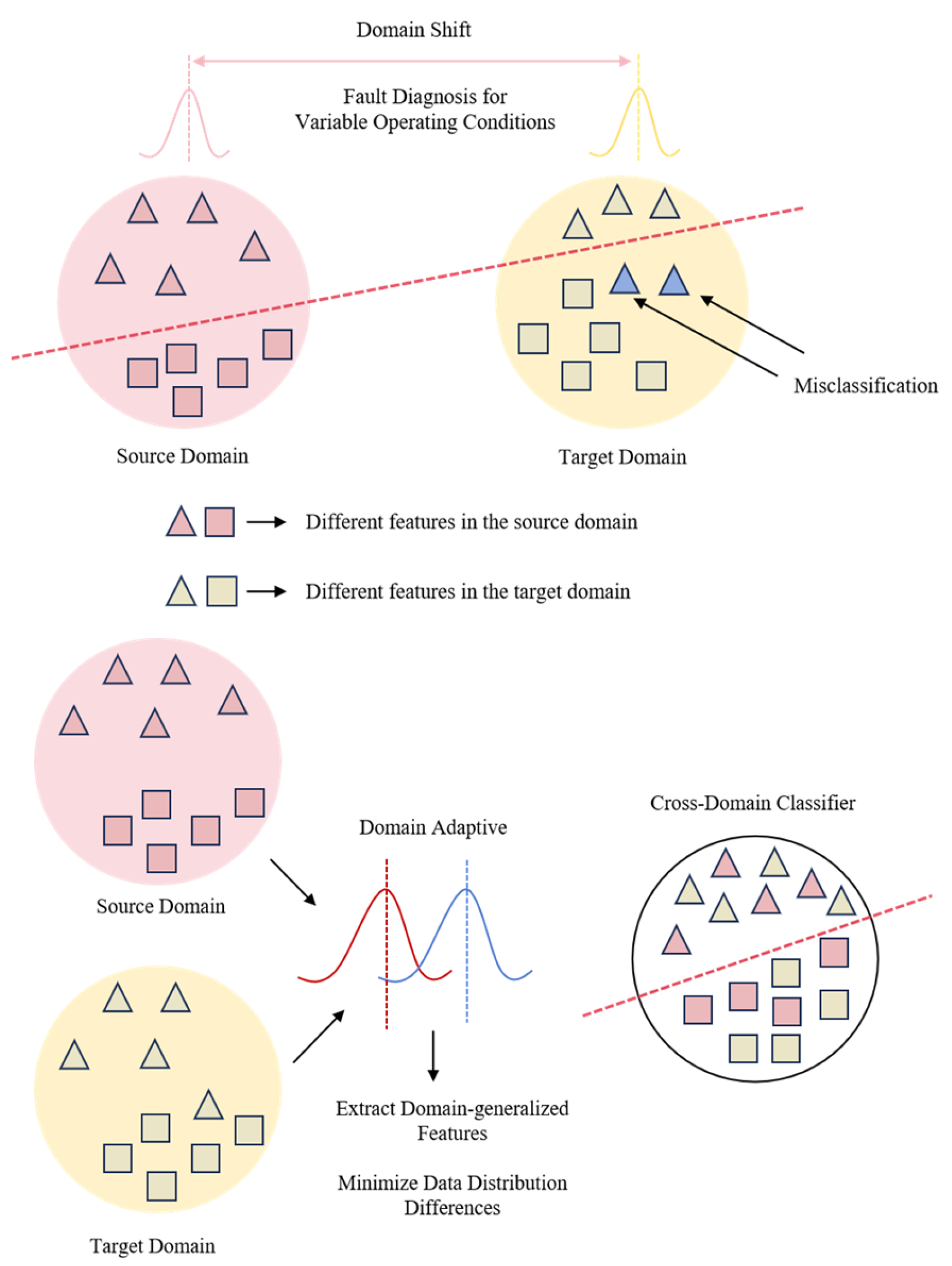
2.1. Unsupervised Domain Adaptation
2.2. Multi-Scale Convolution
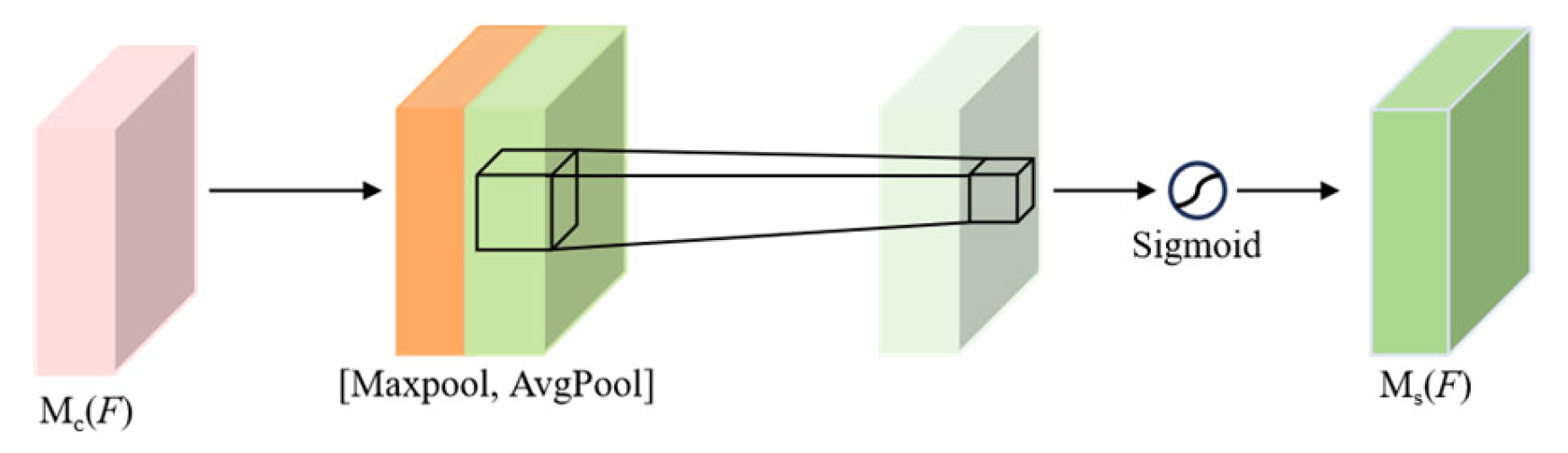
2.3. Convolutional Block Attention Module
2.4. JMMD and CORAL
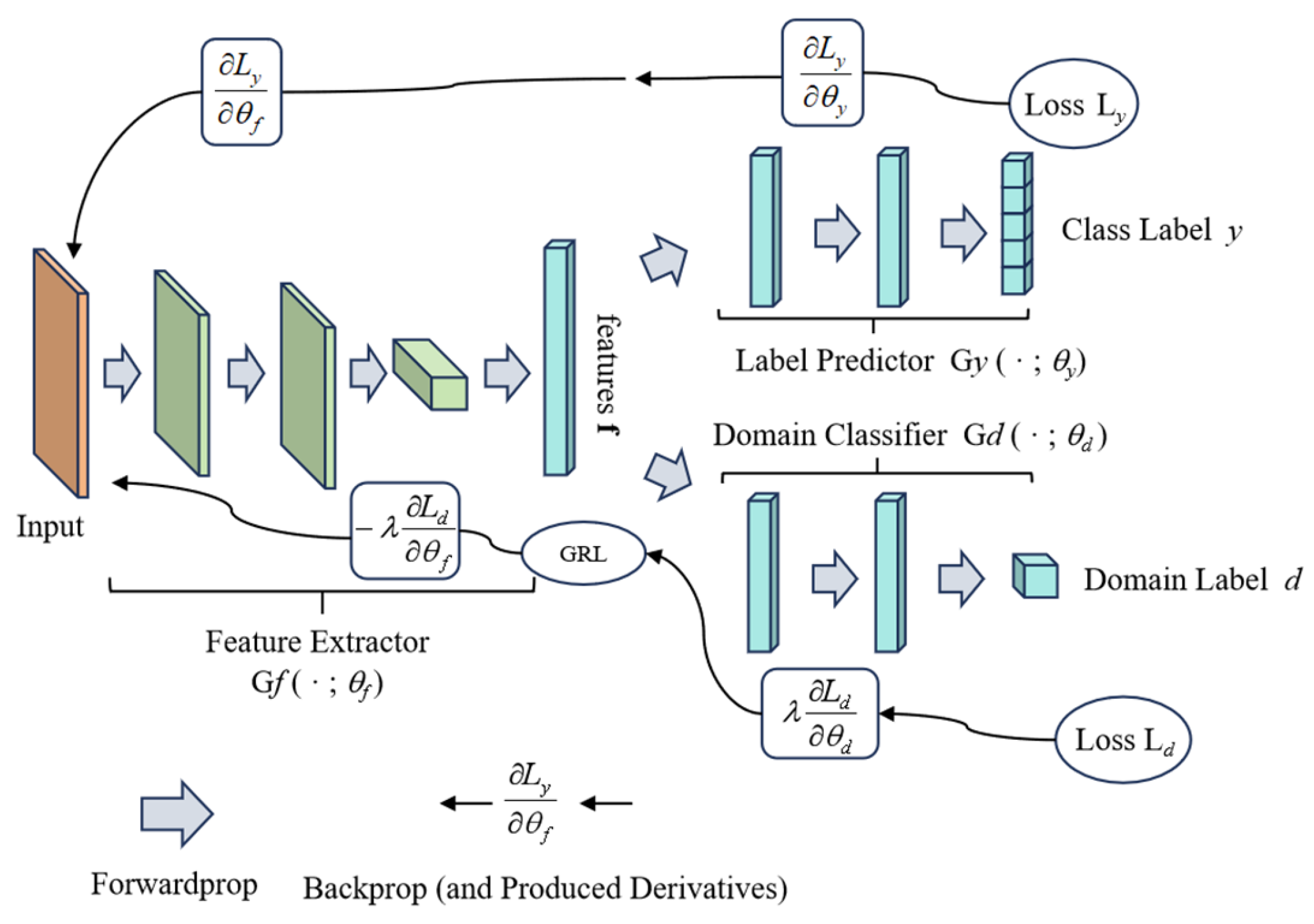
2.5. DANN
3. Bearing Fault Diagnosis Model Based on Migration Learning
4. Results
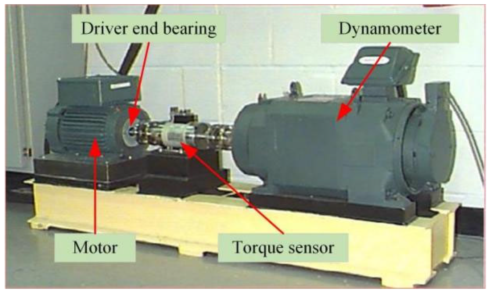
4.1. Introduction to the Experimental Setup and Open Bearing Dataset
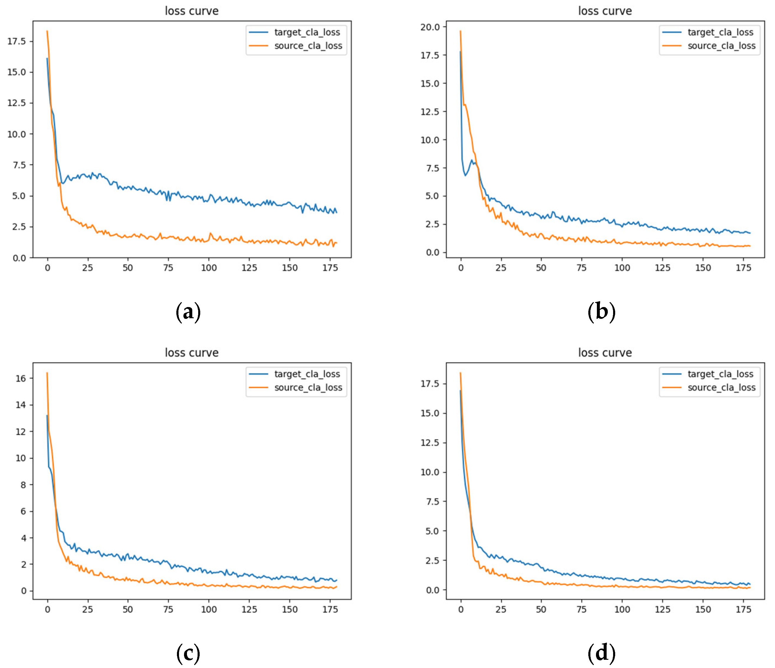
4.2. Comparative Experiments and Analysis of Results
4.3. Ablation Experiment and Result Analysis
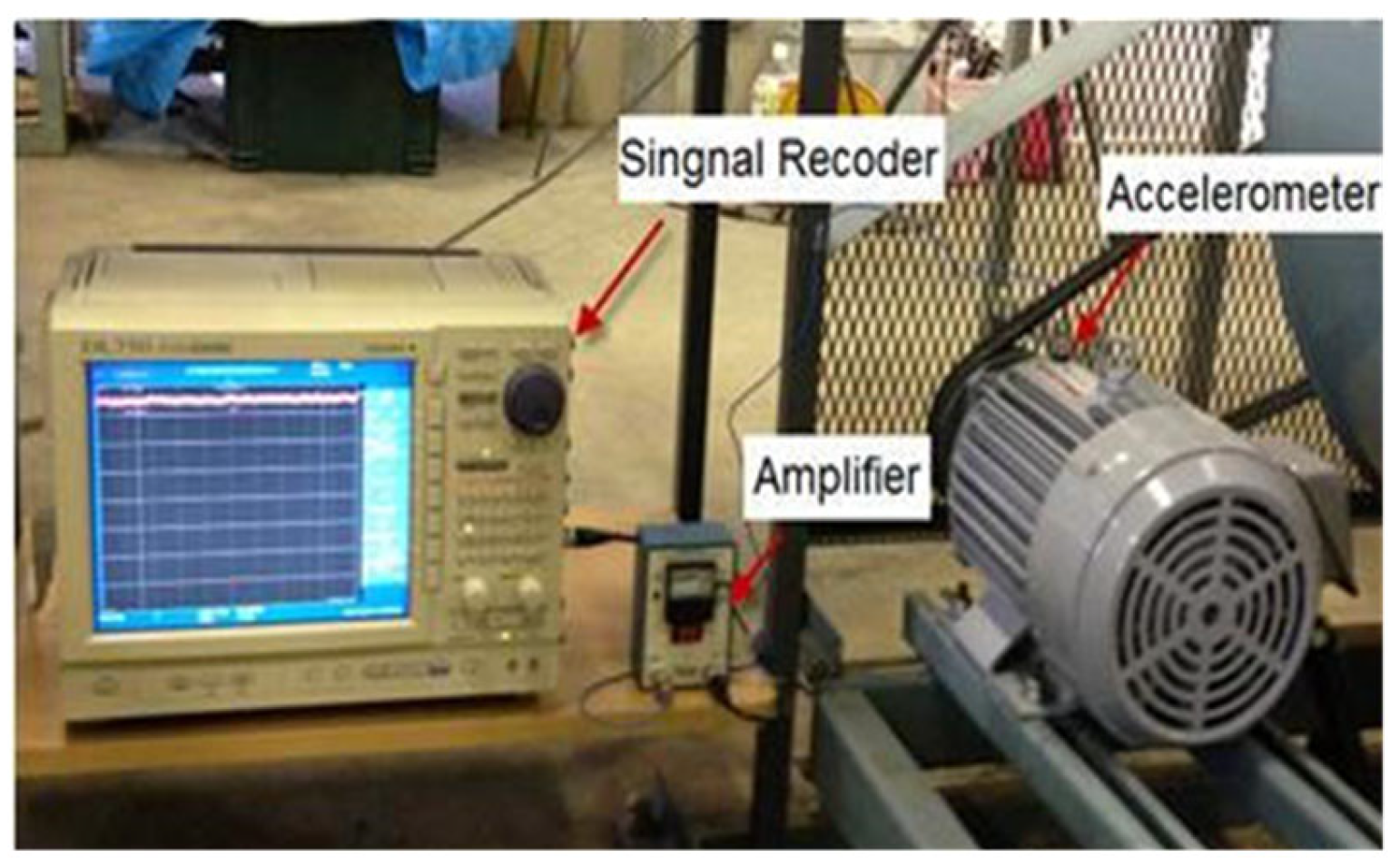
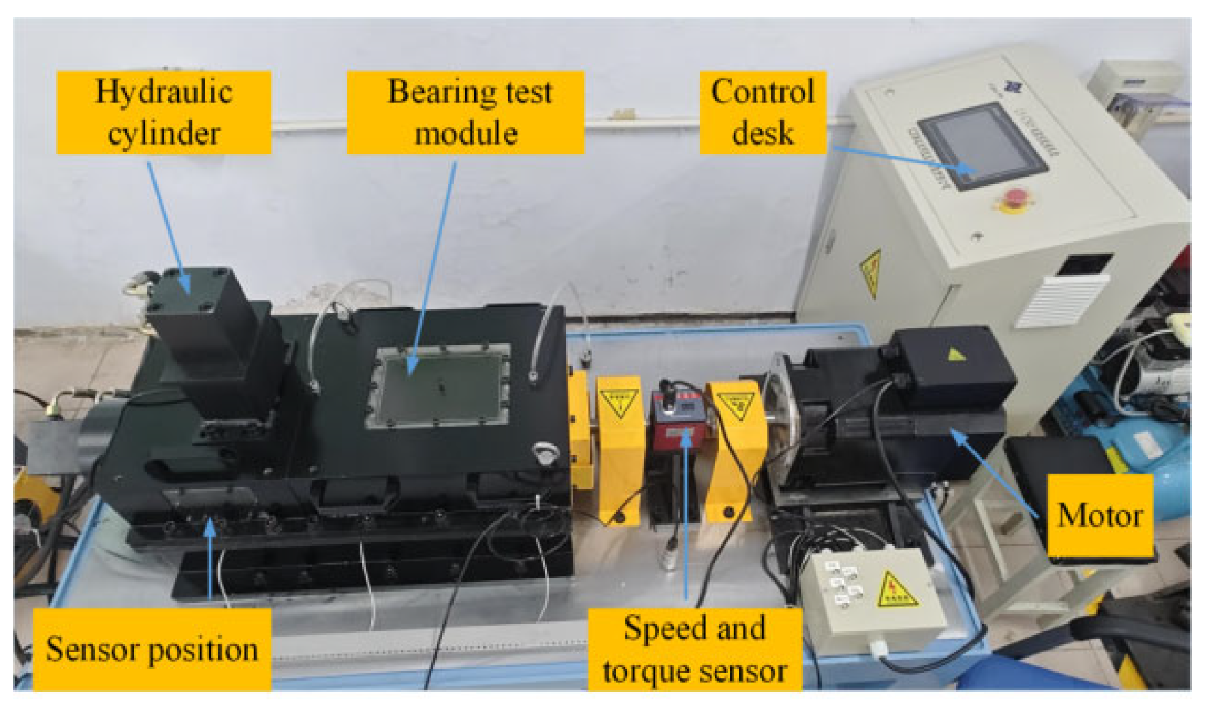
4.4. Introduction to the Experimental Setup and Our Laboratory Bearing Dataset
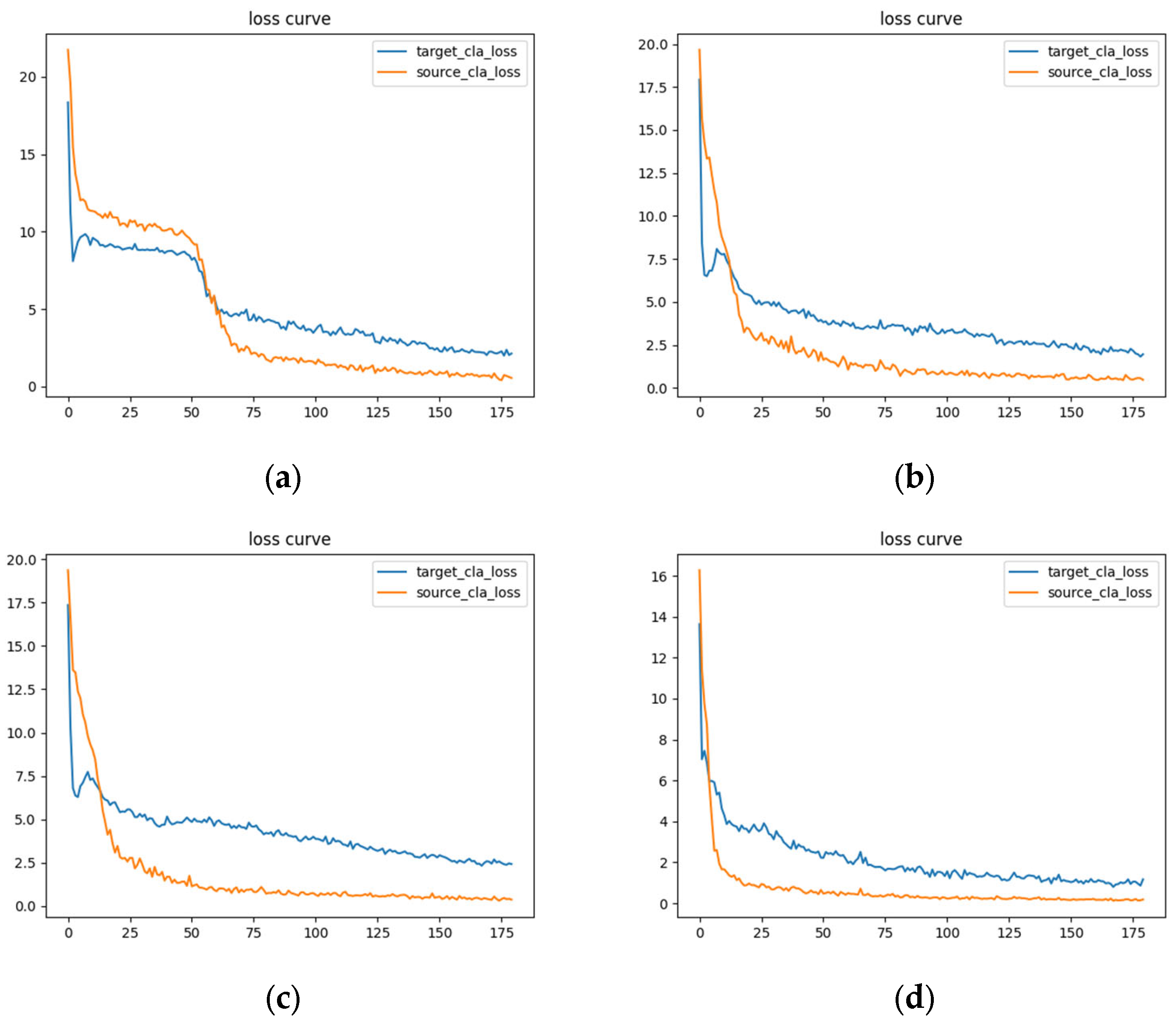
4.5. Experimental Results and Analysis
5. Discussion
Author Contributions
Funding
Institutional Review Board Statement
Informed Consent Statement
Data Availability Statement
Conflicts of Interest
Abbreviations
References
- Tian, J.; Jiang, Y.; Zhang, J.; Luo, H.; Yin, S. A novel data augmentation approach to fault diagnosis with class-imbalance problem. Reliab. Eng. Syst. Saf. 2024, 243, 109832. [Google Scholar] [CrossRef]
- Lu, W.; Liu, J.; Lin, F. The Fault Diagnosis of Rolling Bearings Is Conducted by Employing a Dual-Branch Convolutional Capsule Neural Network. Sensors 2024, 24, 3384. [Google Scholar] [CrossRef] [PubMed]
- Zhong, S.; Fu, S.; Lin, L. A novel gas turbine fault diagnosis method based on transfer learning with CNN. Measurement 2019, 137, 435–453. [Google Scholar] [CrossRef]
- Yang, X.; Yang, J.; Jin, Y.; Liu, Z. A New Method for Bearing Fault Diagnosis across Machines Based on Envelope Spectrum and Conditional Metric Learning. Sensors 2024, 24, 2674. [Google Scholar] [CrossRef] [PubMed]
- Wang, Y.; Liang, J.; Gu, X.; Ling, D.; Yu, H. Multi-scale attention mechanism residual neural network for fault diagnosis of rolling bearings. Proc. Inst. Mech. Eng. Part C J. Mech. Eng. Sci. 2022, 236, 10615–10629. [Google Scholar] [CrossRef]
- Li, Y.; Gu, X.; Wei, Y. A Deep Learning-Based Method for Bearing Fault Diagnosis with Few-Shot Learning. Sensors 2024, 24, 7516. [Google Scholar] [CrossRef]
- Zhu, H.; Sui, Z.; Xu, J.; Lan, Y. Fault Diagnosis of Mechanical Rolling Bearings Using a Convolutional Neural Network–Gated Recurrent Unit Method with Envelope Analysis and Adaptive Mean Filtering. Processes 2024, 12, 2845. [Google Scholar] [CrossRef]
- Li, X.; Chen, J.; Wang, J.; Wang, J.; Li, X.; Kan, Y. Research on Fault Diagnosis Method of Bearings in the Spindle System for CNC Machine Tools Based on DRSN-Transformer. IEEE Access 2024, 12, 74586–74595. [Google Scholar] [CrossRef]
- Li, X.; Chen, J.; Wang, J.; Wang, J.; Wang, J.; Li, X.; Kan, Y. Multi-Scale Channel Mixing Convolutional Network and Enhanced Residual Shrinkage Network for Rolling Bearing Fault Diagnosis. Electronics 2025, 14, 855. [Google Scholar] [CrossRef]
- Chen, X.; Zhang, B.; Gao, D. Bearing fault diagnosis base on multi-scale CNN and LSTM model. J. Intell. Manuf. 2021, 32, 971–987. [Google Scholar] [CrossRef]
- Li, T.; Zhao, Z.; Sun, C.; Cheng, L.; Chen, X.; Yan, R.; Gao, R.X. Wavelet Kernel Net: An interpretable deep neural network for industrial intelligent diagnosis. IEEE Trans. Syst. Man Cybern. Syst. 2021, 52, 2302–2312. [Google Scholar] [CrossRef]
- Liu, X.; Chen, J.; Zhang, K.; Liu, S.; He, S.; Zhou, Z. Cross-domain intelligent bearing fault diagnosis under class imbalanced samples via transfer residual network augmented with explicit weight self-assignment strategy based on meta data. Knowl. Based Syst. 2022, 251, 109272. [Google Scholar] [CrossRef]
- Kumar, P.; Kumar, P.; Hati, A.S.; Kim, H.S. Deep transfer learning framework for bearing fault detection in motors. Mathematics 2022, 10, 4683. [Google Scholar] [CrossRef]
- Kuang, J.; Xu, G.; Tao, T.; Wu, Q. Class-imbalance adversarial transfer learning network for cross-domain fault diagnosis with imbalanced data. IEEE Trans. Instrum. Meas. 2021, 71, 1–11. [Google Scholar] [CrossRef]
- Tong, Z.; Li, W.; Zhang, B.; Jiang, F.; Zhou, G. Bearing Fault Diagnosis Under Variable Working Conditions Based on Domain Adaptation Using Feature Transfer Learning. IEEE Access 2018, 6, 76187–76197. [Google Scholar] [CrossRef]
- Azamfar, M.; Singh, J.; Li, X.; Lee, J. Cross-domain Gearbox Diagnostics under Variable Working Conditions with Deep Convolutional Transfer Learning. J. Vib. Control 2021, 27, 854–864. [Google Scholar] [CrossRef]
- Li, X.; Zhang, W.; Ding, Q.; Sun, J.-Q. Multi-Layer domain adaptation method for rolling bearing fault diagnosis. Signal Process. 2019, 157, 180–197. [Google Scholar] [CrossRef]
- An, J.; Ai, P.; Liu, D. Deep domain adaptation model for bearing fault diagnosis with domain alignment and discriminative feature learning. Shock Vib. 2020, 2020, 4676701. [Google Scholar] [CrossRef]
- Han, T.; Liu, C.; Yang, W.; Jiang, D. Deep Transfer Network with Joint Distribution Adaptation: A New Intelligent Fault Diagnosis Framework for Industry Application. ISA Trans. 2020, 97, 269–281. [Google Scholar] [CrossRef]
- Zhao, K.; Jiang, H.; Wang, K.; Pei, Z. Joint Distribution Adaptation Network with Adversarial Learning for Rolling Bearing Fault Diagnosis. Knowl. Based Syst. 2021, 222, 106–117. [Google Scholar] [CrossRef]
- Xiao, Y.; Shao, H.; Han, S.; Huo, Z.; Wan, J. Novel joint transfer network for unsupervised bearing fault diagnosis from simulation domain to experimental domain. IEEE/ASME Trans. Mechatron. 2022, 27, 5254–5263. [Google Scholar] [CrossRef]
- Zhao, X.; Wang, L.; Zhang, Y.; Han, X.; Deveci, M.; Parmar, M. A review of convolutional neural networks in computer vision. Artif. Intell. Rev. 2024, 57, 99. [Google Scholar] [CrossRef]
- Yang, Y.; Zhang, T.; Li, G.; Kim, T.; Wang, G. An unsupervised domain adaptation model based on dual-module adversarial training. Neurocomputing 2022, 475, 102–111. [Google Scholar] [CrossRef]
- Xu, Y.; Liu, J.; Wan, Z.; Zhang, D.; Jiang, D. Rotor fault diagnosis using domain-adversarial neural network with time-frequency analysis. Machines 2022, 10, 610. [Google Scholar] [CrossRef]
- Zhang, W.; Wu, D. Discriminative joint probability maximum mean discrepancy (DJP-MMD) for domain adaptation. In Proceedings of the 2020 International Joint Conference on Neural Networks (IJCNN), Glasgow, UK, 19–24 July 2020; IEEE: New York, NY, USA, 2020; pp. 1–8. [Google Scholar]
- Zhu, Y.; Zhuang, F.; Wang, J.; Ke, G.; Chen, J.; Bian, J.; Xiong, H.; He, Q. Deep subdomain adaptive networks for image classification. IEEE Trans. Neural Netw. Learn. Syst. 2020, 32, 1713–1722. [Google Scholar] [CrossRef]
- Wang, Z.; Ming, X. A Domain Adaptation Method Based on Deep Coral for Rolling Bearing Fault Diagnosis. In Proceedings of the 2023 IEEE 14th International Symposium on Diagnostics for Electrical Machines, Power Electronics and Drives (SDEMPED), Chania, Greece, 28–31 August 2023; IEEE: New York, NY, USA, 2023; pp. 211–216. [Google Scholar]


| Layers | Components | Tied Parameters | Padding |
|---|---|---|---|
| Layer1 | Conv1 | Kernels: 64 × 1 × 32, stride: 16 | 24 |
| BN | 32 | / | |
| ReLU | / | / | |
| Maxpool 1 | 2 | / | |
| Layer2 | Conv2 | Kernels: 32 × 1 × 32, stride: 16 | 16 |
| BN | 32 | / | |
| ReLU | / | / | |
| Maxpool 2 | 2 | / | |
| Layer3 | Conv3 | Kernels: 16 × 1 × 32, stride: 16 | 8 |
| BN | 32 | / | |
| ReLU | / | / | |
| Maxpool 3 | 2 | / | |
| CBAM | / | 96 | / |
| FC1 | / | 96 × 512 | / |
| FC2 | / | 512 × 4 | / |
| Type of Data Set | Type of Fault | Frequency | Speed (r/min) | Load/(Hp) | Fault Size | Sample Size | Tab |
|---|---|---|---|---|---|---|---|
| CWRU | NC | 12 kHz | 1750 | 2 | 0 | 1000 | 0 |
| IF | 1750 | 2 | 0.007 inch. | 1000 | 1 | ||
| OF | 1750 | 2 | 0.007 inch. | 1000 | 2 | ||
| BF | 1750 | 2 | 0.007 inch. | 1000 | 3 | ||
| JNU | N | 50 kHz | 600 | / | / | 1000 | 0 |
| IB | 600 | / | / | 1000 | 1 | ||
| OB | 600 | / | / | 1000 | 2 | ||
| TB | 600 | / | / | 1000 | 3 | ||
| N | 800 | / | / | 1000 | 0 | ||
| IB | 800 | / | / | 1000 | 1 | ||
| OB | 800 | / | / | 1000 | 2 | ||
| TB | 800 | / | / | 1000 | 3 | ||
| N | 1000 | / | / | 1000 | 0 | ||
| IB | 1000 | / | / | 1000 | 1 | ||
| OB | 1000 | / | / | 1000 | 2 | ||
| TB | 1000 | / | / | 1000 | 3 |
| Migration Tasks | MMD | DC | DANN | DSAN | Method of This Paper |
|---|---|---|---|---|---|
| A1 → B1 | 82.83 ± 1.42% | 91.57 ± 0.95% | 93.97 ± 1.18% | 94.25 ± 0.92% | 98.65 ± 0.41% |
| A1 → C1 | 82.75 ± 1.44% | 92.90 ± 0.96% | 92.15 ± 1.20% | 93.72 ± 0.92% | 99.50 ± 0.43% |
| A1 → D1 | 84.75 ± 1.43% | 92.15 ± 0.96% | 93.95 ± 1.19% | 95.37 ± 0.94% | 98.60 ± 0.42% |
| B1 → A1 | 84.33 ± 1.43% | 93.17 ± 0.95% | 93.80 ± 1.19% | 93.35 ± 0.92% | 98.17 ± 0.41% |
| B1 → C1 | 85.35 ± 1.42% | 94.72 ± 0.96% | 92.87 ± 1.18% | 94.20 ± 0.92% | 98.45 ± 0.41% |
| B1 → D1 | 82.82 ± 1.43% | 92.70 ± 0.97% | 90.97 ± 1.18% | 95.60 ± 0.93% | 97.87 ± 0.43% |
| C1 → A1 | 81.52 ± 1.44% | 92.22 ± 0.96% | 92.07 ± 1.20% | 94.47 ± 0.92% | 98.50 ± 0.42% |
| C1 → B1 | 86.15 ± 1.42% | 91.42 ± 0.95% | 91.62 ± 1.18% | 95.30 ± 0.91% | 99.27 ± 0.42% |
| C1 → D1 | 85.00 ± 1.42% | 91.60 ± 0.95% | 90.07 ± 1.19% | 96.25 ± 0.93% | 99.32 ± 0.41% |
| D1 → A1 | 83.25 ± 1.43% | 91.72 ± 0.97% | 92.62 ± 1.20% | 94.80 ± 0.94% | 98.57 ± 0.43% |
| D1 → B1 | 85.15 ± 1.43% | 91.97 ± 0.95% | 92.87 ± 1.18% | 93.92 ± 0.92% | 98.80 ± 0.41% |
| D1 → C1 | 84.90 ± 1.42% | 92.00 ± 0.96% | 92.21 ± 1.18% | 93.25 ± 0.92% | 99.33 ± 0.41% |
| Average Value | 84.07 | 92.35 | 92.43 | 94.54 | 98.75 |
| Migration Tasks A1 → D1 | MMD | DC | DANN | DSAN | Method of This Paper |
|---|---|---|---|---|---|
| Accuracy | 84.75 ± 1.43% | 92.15 ± 0.96% | 93.95 ± 1.19% | 95.37 ± 0.94% | 98.60 ± 0.42% |
| Runtime | 0.058 s | 0.098 s | 0.113 s | 0.173 s | 0.105 s |
| Migration Tasks | Experiment 1 | Experiment 2 | Experiment 3 | Experiment 4 | Experiment 5 | Method of This Paper |
|---|---|---|---|---|---|---|
| A1 → B1 | 86.80 ± 0.74% | 94.87 ± 0.54% | 91.32 ± 0.93% | 92.62 ± 0.61% | 95.95 ± 0.52% | 98.65 ± 0.41% |
| A1 → C1 | 84.70 ± 0.75% | 93.97 ± 0.56% | 90.67 ± 0.95% | 92.55 ± 0.63% | 95.70 ± 0.52% | 99.50 ± 0.43% |
| A1 → D1 | 84.95 ± 0.75% | 94.35 ± 0.54% | 90.13 ± 0.93% | 92.75 ± 0.62% | 96.53 ± 0.53% | 98.60 ± 0.42% |
| B1 → A1 | 85.32 ± 0.74% | 94.07 ± 0.55% | 90.87 ± 0.93% | 93.12 ± 0.61% | 95.15 ± 0.52% | 98.17 ± 0.41% |
| B1 → C1 | 85.15 ± 0.74% | 94.53 ± 0.55% | 90.05 ± 0.94% | 93.10 ± 0.61% | 95.87 ± 0.53% | 98.45 ± 0.41% |
| B1 → D1 | 84.75 ± 0.76% | 94.45 ± 0.54% | 90.30 ± 0.94% | 92.22 ± 0.62% | 94.97 ± 0.52% | 97.87 ± 0.43% |
| C1 → A1 | 84.73 ± 0.76% | 94.12 ± 0.56% | 90.75 ± 0.95% | 92.67 ± 0.63% | 95.62 ± 0.54% | 98.50 ± 0.42% |
| C1 → B1 | 85.02 ± 0.75% | 93.95 ± 0.55% | 90.27 ± 0.95% | 93.12 ± 0.62% | 96.72 ± 0.52% | 99.27 ± 0.42% |
| C1 → D1 | 84.15 ± 0.74% | 93.71 ± 0.56% | 91.97 ± 0.94% | 92.82 ± 0.62% | 96.22 ± 0.53% | 99.32 ± 0.41% |
| D1 → A1 | 84.72 ± 0.75% | 93.75 ± 0.56% | 90.60 ± 0.95% | 92.02 ± 0.61% | 95.72 ± 0.53% | 98.57 ± 0.43% |
| D1 → B1 | 85.02 ± 0.76% | 94.37 ± 0.54% | 90.47 ± 0.94% | 91.97 ± 0.63% | 95.95 ± 0.54% | 98.80 ± 0.41% |
| D1 → C1 | 85.61 ± 0.75% | 94.27 ± 0.55% | 91.22 ± 0.93% | 92.17 ± 0.62% | 96.61 ± 0.53% | 99.33 ± 0.41% |
| Average Value | 85.08 | 94.20 | 90.72 | 92.59 | 95.92 | 98.75 |
| Migration Tasks A1 → D1 | Experiment 1 | Experiment 2 | Experiment 3 | Experiment 4 | Experiment 5 | Method of This Paper |
|---|---|---|---|---|---|---|
| Accuracy | 84.95 ± 0.75% | 94.35 ± 0.54% | 90.13 ± 0.93% | 92.75 ± 0.62% | 96.53 ± 0.53% | 98.60 ± 0.42% |
| Runtime | 0.143 s | 0.063 s | 0.023 s | 0.095 s | 0.081 s | 0.105 s |
| Frequency | SNR/dB | Speed/(r/min) | Tab |
|---|---|---|---|
| A2 | NF | 800 | 0 |
| IF | 1 | ||
| OF | 2 | ||
| BF | 3 | ||
| B2 | NF | 1200 | 0 |
| IF | 1 | ||
| OF | 2 | ||
| BF | 3 | ||
| C2 | NF | 1600 | 0 |
| IF | 1 | ||
| OF | 2 | ||
| BF | 3 | ||
| D2 | NF | 2000 | 0 |
| IF | 1 | ||
| OF | 2 | ||
| BF | 3 |
| Migration Tasks | MMD | DC | DANN | DSAN | Method of This Paper |
|---|---|---|---|---|---|
| A2 → B2 | 85.12 ± 1.37% | 91.15 ± 1.05 | 92.67 ± 0.94 | 93.30 ± 0.72 | 99.42 ± 0.51 |
| A2 → C2 | 83.62 ± 1.38% | 92.95 ± 1.07 | 92.72 ± 0.94 | 95.25 ± 0.71 | 97.55 ± 0.52 |
| A2 → D2 | 82.77 ± 1.38% | 91.82 ± 1.06 | 92.60 ± 0.95 | 94.67 ± 0.71 | 98.52 ± 0.52 |
| B2 → A2 | 85.20 ± 1.37% | 91.15 ± 1.05 | 94.52 ± 0.94 | 94.37 ± 0.73 | 99.70 ± 0.51 |
| B2 → C2 | 86.45 ± 1.37% | 92.90 ± 1.05 | 93.90 ± 0.96 | 93.75 ± 0.72 | 97.87 ± 0.52 |
| B2 → D2 | 82.77 ± 1.39% | 91.92 ± 1.07 | 93.57 ± 0.96 | 94.80 ± 0.71 | 96.53 ± 0.51 |
| C2 → A2 | 85.40 ± 1.38% | 89.85 ± 1.06 | 92.72 ± 0.95 | 94.92 ± 0.72 | 98.30 ± 0.53 |
| C2 → B2 | 81.70 ± 1.37% | 90.62 ± 1.05 | 90.05 ± 0.94 | 93.55 ± 0.71 | 99.27 ± 0.51 |
| C2 → D2 | 85.60 ± 1.37% | 91.02 ± 1.05 | 93.90 ± 0.94 | 95.57 ± 0.73 | 98.92 ± 0.51 |
| D2 → A2 | 83.97 ± 1.39% | 90.92 ± 1.07 | 91.65 ± 0.96 | 94.77 ± 0.72 | 99.17 ± 0.53 |
| D2 → B2 | 84.67 ± 1.37% | 90.85 ± 1.05 | 92.40 ± 0.94 | 93.82 ± 0.71 | 99.35 ± 0.51 |
| D2 → C2 | 83.21 ± 1.38% | 93.40 ± 1.05 | 93.07 ± 0.95 | 94.17 ± 0.73 | 98.30 ± 0.51 |
| Average Value | 84.21 | 91.55 | 92.81 | 94.41 | 98.58 |
Disclaimer/Publisher’s Note: The statements, opinions and data contained in all publications are solely those of the individual author(s) and contributor(s) and not of MDPI and/or the editor(s). MDPI and/or the editor(s) disclaim responsibility for any injury to people or property resulting from any ideas, methods, instructions or products referred to in the content. |
© 2025 by the authors. Licensee MDPI, Basel, Switzerland. This article is an open access article distributed under the terms and conditions of the Creative Commons Attribution (CC BY) license (https://creativecommons.org/licenses/by/4.0/).
Share and Cite
Li, X.; Wang, J.; Wang, J.; Wang, J.; Li, Q.; Yu, X.; Chen, J. Research on Unsupervised Domain Adaptive Bearing Fault Diagnosis Method Based on Migration Learning Using MSACNN-IJMMD-DANN. Machines 2025, 13, 618. https://doi.org/10.3390/machines13070618
Li X, Wang J, Wang J, Wang J, Li Q, Yu X, Chen J. Research on Unsupervised Domain Adaptive Bearing Fault Diagnosis Method Based on Migration Learning Using MSACNN-IJMMD-DANN. Machines. 2025; 13(7):618. https://doi.org/10.3390/machines13070618
Chicago/Turabian StyleLi, Xiaoxu, Jiahao Wang, Jianqiang Wang, Jixuan Wang, Qinghua Li, Xuelian Yu, and Jiaming Chen. 2025. "Research on Unsupervised Domain Adaptive Bearing Fault Diagnosis Method Based on Migration Learning Using MSACNN-IJMMD-DANN" Machines 13, no. 7: 618. https://doi.org/10.3390/machines13070618
APA StyleLi, X., Wang, J., Wang, J., Wang, J., Li, Q., Yu, X., & Chen, J. (2025). Research on Unsupervised Domain Adaptive Bearing Fault Diagnosis Method Based on Migration Learning Using MSACNN-IJMMD-DANN. Machines, 13(7), 618. https://doi.org/10.3390/machines13070618