Abstract
In the era of rapid industrial automation advancements, the complexity of intelligent manufacturing equipment has been steadily escalated. Stringent demands for high-efficiency and high-precision diagnosis are increasingly being unmet by conventional fault diagnosis methods. To address these challenges, a novel fault diagnosis approach grounded in quantum Q-learning is presented in this paper. The distinct advantages of quantum computing are innovatively integrated with the decision-making framework of Q-learning through this method. By harnessing the multi-information-carrying capacities of qubits, vast amounts of multi-source heterogeneous data generated during equipment operation can be efficiently processed. Latent fault features are thereby rapidly uncovered, significantly reducing the time required for fault-feature extraction. Furthermore, optimal decisions can be dynamically formulated by Q-learning within evolving production environments, leveraging precise analysis outcomes from quantum computing. Real-time equipment status is continuously monitored to accurately identify fault types, pinpoint locations, and promptly generate targeted maintenance strategies. Fault-diagnosis tests conducted on typical industrial intelligent manufacturing equipment demonstrate that the quantum Q-learning method outperforms traditional approaches in terms of diagnosis accuracy, efficiency, and adaptability to complex fault patterns. This breakthrough opens up new frontiers for fault diagnosis in intelligent manufacturing systems.
1. Introduction
Intelligent manufacturing [1,2] has emerged as a pivotal trend in advanced industries. As the foundational infrastructure of this transformation, intelligent manufacturing equipment must operate with stability and reliability, which is essential to ensuring system integrity and maintaining operational efficiency. However, as automation technology advances rapidly, the structure of intelligent manufacturing equipment has grown increasingly complex, while its operating environment has become more dynamic—particularly in high-end precision manufacturing sectors like aerospace components and high-performance chip production [3]. The equipment integrates a large number of the precision components, involves multi-disciplinary integration, and needs to operate continuously and stably under harsh conditions. This has brought to intelligent manufacturing equipment the unprecedented challenges of monitoring, operation, and maintenance. The traditional fault diagnosis method based on a single sensor and simple threshold judgment can hardly capture the subtle faults early [4,5]. Once the intelligent manufacturing equipment fails or stops, the loss of production suspension per minute or even per second may be substantial, which brings great economic pressure to enterprises, and also seriously affects the collaborative promotion of the entire industrial chain. Therefore, timely and accurate fault diagnosis for intelligent manufacturing equipment is crucial to minimizing downtime, reducing maintenance costs, and improving production efficiency. Proactive anomaly detection and resolution can substantially enhance system reliability while ensuring operational continuity in intelligent manufacturing equipment. Currently established fault diagnosis methodologies mainly fall into three categories: signal processing-based approaches [6], knowledge-based systems [7], and machine learning algorithms [8]. Although these techniques have proven effective to varying degrees in diagnosing conventional industrial equipment anomalies, they exhibit inherent limitations when applied to contemporary intelligent manufacturing systems.
The fault diagnosis methodologies based on signal processing are primarily concerned with the acquisition, analysis, and manipulation of diverse operational signals (including vibration, acoustic, and current signals among others). The feature extraction is performed to identify signatures indicative of the equipment’s operational state, followed by automated fault detection and classification to determine the presence, type, and severity of anomalies. Fault diagnosis and analysis of rotating machinery was conducted in [9] through the application of signal processing techniques and lightweight methodologies, incorporating mechanical structural characteristics for feature extraction and anomaly detection. The fault diagnosis of distribution network was studied in [10] based on artificial intelligence and signal processing technology.
Although the above efforts have successfully implemented fault diagnosis for diverse mechanical systems through the application of signal processing techniques, this methodological framework inherently faces significant challenges in addressing modern industrial requirements. The signal processing fault diagnosis technology has limited complex signal processing capability and insufficient noise resistance, so it has difficulty dealing with non-stationary, non-linear and multi-source signals, and it is also vulnerable to non-Gaussian noise and low signal-to-noise ratio. Moreover, the signal processing fault diagnosis technology generalizability is limited, and it is difficult to adapt to the working condition changes of intelligent manufacturing equipment. It can only extract shallow features, and it has poor ability.
However, knowledge-based fault diagnosis methods offer distinct advantages in addressing these limitations. In [11], the fault diagnosis method based on knowledge achieved good performance on rolling bearings without the need for fault sample training. The method of self-supervised learning based on prior knowledge in [12] achieved the diagnosis of intelligent bearing faults with a small number of fault samples. However, in practical engineering scenarios, the knowledge-based fault diagnosis methods often encounter challenges due to the inherent difficulties in knowledge acquisition, coupled with the limitations of the acquired knowledge. These factors significantly restrict their capacity to effectively address emerging fault patterns in real-world applications.
The Q-learning method can interact with the environment through agents and continuously learn the optimal strategy to maximize the cumulative reward, and has been applied in the fault management in various industries. An adaptive fault diagnosis and classification approach for large-capacity low-inertia power systems was proposed in [13] through the utilization of machine learning techniques and phasor measurement unit (PMU) data. Effective immune biomarkers for the diagnosis and classification of alopecia areata were identified in [14] using Q-learning techniques, complemented by correlation analysis between core genes and key biomarker genes. However, traditional Q-learning algorithms exhibit significant limitations in addressing high-dimensional state spaces and complex decision-making tasks, primarily due to their computational inefficiency and slow convergence speed. This restricts their applicability in modern intelligent manufacturing systems characterized by complex operational environments and rapid dynamic requirements. Quantum computing, in contrast, offers distinctive advantages through quantum parallelism and entanglement, which have been theoretically proven to exponentially enhance computational efficiency for complex problem-solving scenarios, as detailed in [15,16]. Therefore, the integration of quantum computing principles with Q-learning frameworks enables the realization of synergistic complementarity, thereby expanding their applicability across diverse industrial sectors as documented in [17,18,19,20]. A quantum Q-learning framework was applied in [21] to optimize real-time resource allocation for electric vehicle charging systems, yielding significant improvements, including reduced charging service time, enhanced service success rate, and minimized operational costs. In [22], a Q-learning approach founded on quantum chains is investigated. This approach models the problem of determining the optimal position and number of particles as a Markov decision process. Subsequently, it employs the proximal policy optimization algorithm to seek the optimal chain construction strategies and structures across various scenarios, thereby attaining optimal energy and state transitions. Nevertheless, in the above references, the quantum Q-learning approaches were presented to optimize industrial control systems without accounting for the multifaceted impacts and specific requirements imposed by system faults. Current quantum Q-learning frameworks predominantly focus on enhancing system performance indices during normal operation, improving computational efficiency, and optimizing resource allocation. Conversely, research on fault diagnosis methodologies integrating quantum Q-learning for intelligent manufacturing systems remains scarcely available in the existing literature. Therefore, in this paper, a quantum Q-learning fault diagnosis method is studied for the intelligent manufacturing equipment.
In the proposed method, the quantum computing and Q-learning work together; this can not only sensitively detect faults in the initial stage and avoid serious losses caused by fault deterioration to production, but also continuously optimize the fault diagnosis and response processes and comprehensively improve the reliability, stability and production efficiency of intelligent manufacturing equipment. The paper makes the following contributions:
- It transcends the limitations of traditional fault diagnosis methodologies through quantum computing, facilitating cross-domain integration and expanding the application scope of fault diagnosis technology. This not only augments the diagnostic accuracy and minimizes misdiagnosis and missed detection, but also bolsters the reliability of the overall system.
- Leveraging the parallel processing capabilities of quantum computing, it drastically curtails the fault diagnosis time for intelligent manufacturing equipment. Consequently, the diagnostic efficiency is remarkably enhanced, aptly catering to the exigencies of time-critical systems.
- By incorporating the feedback mechanism inherent in Q-learning, the diagnosis strategy can be dynamically optimized in light of the real-time system status and past diagnostic outcomes. This actualizes the intelligence and adaptability of the diagnostic processes, endowing it with the flexibility to adeptly respond to diverse operating conditions and environmental fluctuations.
2. Principles and Algorithms of Quantum Q-Learning
2.1. Quantum Computing
Quantum computing, emerging as a revolutionary computing paradigm, offers an innovative avenue for resolving intricate computational conundrums. At its heart lie several pivotal concepts, namely qubits, quantum superposition, and quantum entanglement. These elements not only constitute the theoretical bedrock upon which quantum computing is built but also endow it with unparalleled advantages, setting it apart from traditional computing methodologies [23,24]. In the realm of quantum computing, the quantum bit, or Qubit for short, serves as the fundamental building block of information and exhibits essential distinctions when compared to the bit in traditional computing. In traditional computing, a bit is only capable of representing two discrete states, namely 0 or 1. In stark contrast, a quantum bit has the remarkable property of being able to exist in a superposition state encompassing both 0 and 1 simultaneously, which can be mathematically formulated as follows:
where is the quantum bit state vector, which is used to describe the quantum state of the quantum bit. are complex numbers, and they satisfy:
where and represent the probabilities of the quantum bit being in the and states, respectively, which means that the quantum bit can store and process multiple pieces of information simultaneously, greatly expanding the representation and processing capabilities of information. and become the ground states of the quantum computation; they are the orthogonal ground states, and together, they constitute a basis for the state space of the quantum bit.
As can be observed from Equations (1) and (2) mentioned above, within the aforementioned quantum computation system, the calculation process is carried out in a sequential manner, where only a single piece of data can be processed at a time. When confronted with a complex engineering problem demanding a solution, this calculation system is compelled to test different solutions one after another, which substantially hampers the speed and operational efficiency of the system. In contrast, quantum superposition represents a crucial characteristic of the qubit. It empowers the quantum system to exist in multiple states concurrently, thereby enabling parallel computing and presenting a significant departure from the limitations of the traditional sequential approach. In practical application, its state equation can be formulated as:
where is the number of qubits in the system, and is the computational basis state of the qubits, . In this context, denotes a complex number. In accordance with Equation (2), it adheres to the following expression as:
It is evident from Equations (3) and (4) that quantum superposition endows qubits with the ability to exist in multiple states simultaneously. This implies that the quantum computing system is capable of concurrently calculating and evaluating multiple pieces of data, thus significantly enhancing computational efficiency.
From another perspective, quantum entanglement pertains to the profound interdependence that exists among the states of multiple qubits, transcending the constraints of time and space. In the remarkable scenario where two qubits are in an entangled state, any measurement conducted on one of them will instantaneously exert an impact on the state of the other qubit. The intricate entangled state of qubits can be formulated as follows:
where denote the complex numbers relevant to quantum entanglement. In accordance with Equation (4), they also fulfill the following expression:
Quantum entanglement endows quantum system computing with potent parallel processing and information transmission capabilities, empowering quantum computing systems to undertake complex computing tasks that are arduous to accomplish in the realm of intelligent manufacturing engineering. Entanglement entropy represents a crucial physical quantity for quantifying the extent of quantum entanglement. When the entanglement entropy registers zero, it implies the absence of entanglement among the unit quanta within the quantum system; conversely, a larger entanglement entropy value signifies a higher degree of entanglement between the unit quanta in the quantum system. To further validate the significance of the entanglement entropy within the practical domain of intelligent manufacturing engineering, herein, the existence of a bipartite quantum system AB is postulated, and is represented in the form of a density matrix. The reduced density matrix of subsystem A can be obtained when the partial trace over subsystem B is taken and can be expressed as:
where Tr( ) signifies the trace operation function. Subsequently, the entanglement entropy of subsystem A can be defined as:
2.2. Principle of Q-Learning Methodology
Q-learning constitutes a significant domain within machine learning [25]. Its primary objective is to tackle the issue of how an agent can, via interaction with the surrounding environment, acquire the optimal behavioral policy, thereby maximizing the cumulative long-term rewards. The fundamental constituents of Q-learning encompass the agent, environment, state, action, reward, and so forth. These elements engage in mutual interaction and formulate the foundational framework of Q-learning [26,27].
A policy delineates the manner in which the agent selects its action within each state. Such a policy can either be deterministic, meaning that the agent’s actions are predictable based on the state, or stochastic, indicating that the agent’s actions involve an element of randomness. Typically, it is employed within Q-learning systems to signify the probability of opting for action a when in state S, and this relationship can be formulated as:
where represents the state at time t, and is the action taken at time t.
Based on the aforementioned formula, the probability of the agent transitioning to the subsequent state upon choosing action a in state S can be defined as follows:
Within the realm of the Q-learning system, drawing upon Equations (9) and (10), the environment transitions to the subsequent state in accordance with the transition probability . Simultaneously, it bestows a reward upon the agent, with the dispensing of this reward being contingent upon the action selected by the agent as well as the current state . This complex interaction can be formulated as:
Naturally, within the framework of a Q-learning system, the agent aggregates all the rewards it garners from a particular point in time t extending into the future. This aggregated reward is denoted as following:
where represents the discount factor. This factor is specifically utilized to mirror the reality that immediate rewards carry greater significance compared to those in the future.
In order to capture the average magnitude of the cumulative reward that an agent attains subsequent to executing a series of actions in state s under a specified policy π, the state value is defined as follows:
where denotes the expectation and symbolizes the state-value function.
During the state-updating process of the agent within the Q-learning algorithm, to effectively characterize the Markov decision making process, the TD learning presented in the formula is employed to define the update of the state-value function:
where is the learning rate.
Likewise, with the aim of representing the anticipated cumulative reward that the agent secures after executing action a from state s while adhering to policy π, the action value is defined as following:
The updating process of the action value function is likewise predicated upon the Bellman equation and TD learning. Consequently, its update formula can be further deduced as follows:
Policy π updates rely on the value function. To generate an updated policy, the greedy policy improvement approach is employed. This updated policy can be defined as follows:
Throughout the Q-learning process, the aforementioned steps are iteratively repeated. As time elapses, the agent continuously updates variables , and in its interaction with the environment, progressively converging towards the discovery of the optimal policy that maximizes the reward.
2.3. Algorithm of Quantum Q-Learning
Quantum Q-learning represents a potent methodology for augmenting the performance and efficacy of traditional Q-learning by capitalizing on the unique capabilities offered by quantum computing. It serves as an efficacious means for resolving intricate decision-making conundrums. At its heart, the core concept entails the infusion of quintessential quantum traits, namely qubits, quantum superposition, and quantum entanglement, into the overarching framework of Q-learning, thereby enabling the quantum-based representation and manipulation of pivotal elements like the state space, action space, and value functions.
Within a quantum Q-learning system, the progression of the quantum state adheres to the principles of quantum mechanics. Assume that at the discrete time t, the state of the system is denoted by . Subsequently, upon executing the action at, the system state can transition to the next novel quantum state in accordance with the quantum dynamics. The process of this evolution can be mathematically formulated as:
where denotes the quantum operator corresponding to the action at. The aforementioned equation encapsulates the temporal variation with respect to time t. Specifically, the action at exerts its influence on the quantum state via thereby giving rise to the quantum state at time t + 1.
In the quantum Q-learning system, the action selection probability is formulated as the square of the modulus of the inner product between two quantum states. Consequently, in line with Equation (10), the probability of opting for action a while in state under quantum policy can be mathematically represented as:
where denotes the quantum state associated with action a, and stands for the quantum policy function.
Owing to the inherent complexity of quantum systems and the extensive diversity of application scenarios, it is infeasible to formulate a fixed expression for the immediate reward function. Instead, it becomes imperative to define the expression in accordance with specific problems and the corresponding environments. Nevertheless, given the dynamic evolution of quantum states and the stochastic nature of action selection, the expectation factor demands careful consideration in the realm of quantum Q-learning. Hence, in this academic paper, the expected total reward accrued by a quantum state over T discrete time periods is defined as:
where represents the immediate reward acquired upon executing action a within the quantum state . Meanwhile, signifies the expected total reward.
The value function of quantum states embodies the anticipated cumulative reward when commencing from quantum state under policy . It offers a long-term assessment of quantum states and is formulated in this paper as follows:
where denotes the value function pertaining to quantum states. In light of the Bellman equation, Equation (21) can be further formulated as:
The quantum action-value function characterizes the expected cumulative reward obtained by executing action a in state and subsequently adhering to policy . It serves to assess the worth of a particular action within a specific state and can be defined as follows:
Here, stands for the quantum action value function. In accordance with the Bellman equation, Equation (23) can be further presented as:
As stated above, Equations (22) and (24) constitute the core of quantum Q-learning. These equations delineate the recursive relationship among values, whereby the value of the current state or the state-action pair at the present moment is computed through the immediate reward and the value of the subsequent state.
Given that the quantum Q-learning algorithm hinges upon the value iteration algorithm, it becomes necessary to perpetually update the original Q value estimation table in light of new information. This enables the Q function to progressively approach its optimal value. The update process of the Q function can be articulated as:
where denotes the original Q-learning Q value estimation, while stands for the new learning experience.
As can be observed from Equations (18)–(25), within the framework of quantum Q-learning, the value function undergoes updating via the evolution of quantum states. During each iteration, the agent employs quantum gate operations to manipulate the quantum state, computes the value functions corresponding to different actions, and subsequently pinpoints the action yielding the maximum value as the optimal one. This innovative approach capitalizes on the parallelism inherent in quantum computing, enabling the simultaneous processing of multiple states and actions, thereby substantially augmenting the speed and efficiency of the iteration process.
The quantum Q-learning framework integrates two core components: the previously described quantum value iteration and a novel quantum policy gradient mechanism. Leveraging quantum superposition and entanglement phenomena, the quantum policy gradient module achieves high-precision gradient estimation, which significantly accelerates convergence toward optimal policy solutions. The corresponding objective function for quantum strategy optimization is formulated as follows to maximize expected rewards:
Here, serves as a parameterized representation of the policy , and denotes the quantum state distribution of the initial state.
With regard to Equation (26), by employing the path integral method, the quantum policy gradient can be further expressed as:
in which Rt represents the cumulative reward starting from the discrete time t, and can be mathematically formulated as follows:
The aforementioned formula derives the policy gradient by computing the gradient of the log probability of the policy and subsequently multiplying it by the cumulative reward. This resultant policy gradient is then utilized to update the policy parameters, aiming to maximize the expected reward.
Based on the foregoing reasoning, it becomes evident that the quantum Q-learning algorithm integrates the superposition and entanglement properties of quantum states from quantum computing into traditional learning paradigms. This integration enables the algorithm to more astutely strike a balance between exploring new information and leveraging existing experience during the learning process. As a result, it significantly broadens the representation space of states and actions. Moreover, it can handle large-scale search problems in complex tasks with greater efficiency. Building upon the aforementioned design, the following section will pioneer a quantum Q-learning fault diagnosis algorithm. This newly devised algorithm will be incorporated into the fault diagnosis of intelligent manufacturing equipment. By capitalizing on the parallelism and entanglement mechanisms intrinsic to quantum Q-learning within the realm of quantum computing, it will expeditiously explore and dissect the complex state space during fault diagnosis, more adeptly handle the uncertainty and ambiguity that plague fault diagnosis, proficiently extract fault features and correlative information, and ultimately enhance the accuracy, reliability, and robustness of fault diagnosis.
3. Design of the Fault Diagnosis Algorithm Grounded in Quantum Q-Learning
In the context of quantum Q-learning for fault diagnosis, the agent is conceived of as a fault diagnosis system. It acquires the operational state information of the equipment via sensors and then determines which diagnostic method or measure to employ based on this acquired information. The environment pertains to the actual working conditions and operations of the smart manufacturing equipment. It will adaptively change in response to the diagnostic actions taken by the agent and provide the agent with a certain reward feedback to signify the quality of the action. The state can encompass various operating parameters of the equipment or, alternatively, the fault symptoms manifested by the equipment. Meanwhile, the action is construed as the behavior that the agent is capable of undertaking in a given state.
3.1. Quantum Q-Learning State Space Definition
In the fault diagnosis of the intelligent manufacturing equipment via quantum Q-learning, enhancing the correlation between operational state data—multidimensional sensor signals (e.g., vibration, temperature, current)—and quantum bits is essential. This improvement can enable quantum computing to process and extract fault features during equipment operation. Consequently, the multi-dimensional sensor signal vector of the intelligent manufacturing equipment can be expressed as:
where represents the measured value of the i-th sensor and i is the number of the sensors in the intelligent manufacturing equipment system.
The encoding map of the multi-dimensional sensor signal vector x to the quantum state can be expressed as:
where represents the encoding function of the i-th feature block; is the entangling operator which is designed to capture the correlation between the different data. is the tensor product, used to describe the state of a composite quantum system.
Assuming that the encoding map in Equation (30) fully incorporates the fault characteristics of the intelligent manufacturing system, and that forms a complete orthogonal basis for the fault modes of the intelligent manufacturing equipment, Equation (30) can be reduced to a quantum state-space expression with fault, as follows:
As can be observed from the aforementioned formula, the normal or faulty conditions of the intelligent manufacturing system are encoded and manifested via the state of the quantum. This allows the quantum Q-learning algorithm to depict the nuanced distinctions and alterations within the system state with enhanced precision. In the face of certain problems entailing continuous states or high degrees of uncertainty, the quantum state representation is capable of seizing the intrinsic traits of the state more accurately. It thereby lays a robust data groundwork for the fault diagnosis of intelligent manufacturing equipment, augmenting both the accuracy of the algorithm in fault diagnosis and its adaptability to diverse environments.
In actual engineering projects, the quantum states are subject to the influence of various natural factors in the working environment of intelligent manufacturing equipment. As a result, they may encounter multiple types of errors, including bit flips, phase flips, and decoherence. The occurrence of these errors can severely undermine the accuracy and reliability of fault diagnosis based on quantum Q-learning. Confronted with such errors, quantum error correction operations prove indispensable. In the practical application scenarios of quantum Q-learning for fault diagnosis, given the presence of irresistible external factors like temperature fluctuations and electromagnetic interference within the intelligent manufacturing equipment system, these factors will induce changes in the quantum state, causing it to deviate from its original correct state. Consequently, the actual quantum state received by the agent is as follows:
where E represents the error operator. In order to rectify the error existing in the quantum state as indicated in (32), a specifically designed encoding operator C is introduced. Through this operator, the quantum state presented in Equation (31) can be converted into an encoded state possessing fault-tolerant capabilities, as illustrated by the following:
In this context, denotes the encoded state corresponding to the actual quantum state. In accordance with Equation (32), the encoded state subsequent to the occurrence of the error can be formulated as:
Supposing that the error correction operation is carried out by means of the error correction operator , the error correction process for the erroneous code-word as shown in (34) can be further illustrated as:
It can be clearly perceived from the above formula that, with the assistance of the quantum error operator, the encoded state marred by errors can be restored to the correct one to the greatest extent possible. In this way, within the quantum Q-learning system, the agent is enabled to make a selection of actions based on the encoded state following quantum error correction, and subsequently attain the optimal reward.
Owing to the intricacy of the working environment for intelligent manufacturing equipment, both the factors that trigger faults and the types of faults involved will be considerably more complex. To guarantee the precision of fault diagnosis for such equipment, this paper calculates the accuracy of fault diagnosis via the confusion matrix presented below as Table 1.

Table 1.
Confusion matrix for faults of intelligent manufacturing equipment.
As can been seen from Table 1, it is a confusion matrix for intelligent manufacturing equipment faults. In Table 1, . TPi denotes the quantity of samples that have been accurately diagnosed as fault type i. FPij indicates the number of samples that, in reality, belong to fault type i but have been erroneously identified as fault type j. FPi represents the count of samples that truly pertain to fault type i yet are wrongly diagnosed as being faulty in general. FNi stands for the number of samples that are actually free of faults but have been inaccurately classified as fault type i. Meanwhile, TN refers to the number of samples that are truly without faults and have been correctly diagnosed as such.
In the course of fault diagnosis predicated on quantum Q-learning, with the aim of circumventing the variance in accuracy that stems from an imbalanced sample size, the accuracy of fault diagnosis founded on quantum Q-learning is herein defined as:
where symbolizes the macro-averaged accuracy of the quantum Q-learning fault diagnosis system. The formula in question takes into full consideration the diagnosis accuracies of all possible fault types that can emerge in the intelligent manufacturing equipment, thus providing a more comprehensive and representative metric. Here, represents the diagnostic accuracy corresponding to fault type i, and can be computed as following:
where denotes the cumulative number of misdiagnosed samples pertaining to the i-th fault.
When diagnosing faults using the quantum Q-learning algorithm, the algorithm must undergo repeated learning and iteration. To guarantee its scientific convergence, a diagnosis accuracy threshold, denoted as , is preset. When the fault diagnosis accuracy in the test dataset or actual application scenario reaches or exceeds this preset target, it signals that the algorithm has fulfilled the requirements for fault diagnosis and can thus be terminated. Given the complexity of the working environment of smart manufacturing equipment, the following section will define a reward function capable of comprehensively evaluating the operating conditions of such equipment.
3.2. Reward Function Definition
In the context of fault diagnosis for intelligent manufacturing equipment, the design of the reward function demands a comprehensive consideration of multiple factors. These encompass not only the precision and timeliness of the diagnosis process but also the associated costs, with the ultimate goal of enabling the agent to arrive at diagnostic decisions that are both highly accurate and operationally efficient. Against this backdrop, this paper formulates the reward as delineated below:
where denote the weights corresponding to diagnosis accuracy, diagnosis time, repair effect, and action cost, respectively; it should be noted that . represents the reward obtained by the agent after taking action a under quantum state .
Through the application of the above formula, the accuracy, efficiency, and economic viability of fault diagnosis in intelligent manufacturing equipment can be enhanced. Specifically, the optimal action selection reward function in quantum learning fault diagnosis method is defined as follows:
where Mn < 0, Mx > 0 are given reward values. Macro-Accuracy is the accurate fault diagnosis rate of the quantum Q-learning system. represents the fault threshold.
In accordance with Equation (39), when the accurate fault diagnosis rate of the quantum Q-learning system falls below the preset value , the reward will be combined with the maximum reward Mx. This superposition serves to reinforce the corresponding state-action pair, thereby promoting its recurrence in subsequent learning processes. Conversely, if the accurate fault diagnosis rate meets or exceeds , the reward function is amalgamated with Mn. Under such circumstances, this particular state-action combination is effectively weakened, reducing the likelihood of its repetition as the learning progresses. The reward value function serves as an assessment of the contribution degree of the action implemented to transition from state to state . Moreover, the design of the action space constitutes a crucial aspect of the fault diagnosis model for intelligent manufacturing equipment based on quantum Q-learning. It dictates the precise actions that the agent is capable of undertaking when confronted with equipment malfunctions.
3.3. Definition of the Action Space in Quantum Q-Learning
In this research paper, each action ai is correlated with a quantum error-corrected encoded state . Consequently, the action space can be depicted as a collection of quantum states, as illustrated below:
It is evident from the aforementioned formula that the action is manifested through the encoded state following quantum correction. This representation holds significant advantages, as it facilitates the analysis and processing of the working state data of intelligent manufacturing equipment by leveraging the unique strengths of quantum computing.
Additionally, drawing on the concept of quantum probability, this paper forges a connection between the encoded state after quantum correction and the actual action selection probability. The likelihood of the agent opting for action ai while in state can be articulated by introducing the probability amplitude. In line with the fundamental principles of quantum mechanics, the action probability is defined as follows:
where represents the probability amplitude, which is typically a complex number.
During the fault diagnosis process within the framework of quantum Q-learning, the probability amplitude in Equation (41) mentioned above undergoes updates in accordance with the interactions between the agent and the environment throughout the learning process. Guided by the principles underlying the Bellman equation, the update formula for the probability amplitude can be defined as follows:
where represents the discount factor, which functions to balance and evaluate the relative significance between future rewards and immediate current rewards. denotes the reward that the agent obtains when executing action while in state . Meanwhile, signifies the probability of transitioning from state to state as a result of executing a particular action .
The formula stated above is predicated on the concept of value function update in the realm of Q-learning. It also incorporates the unique characteristics of quantum probability amplitudes. This enables the agent to adaptively adjust the probability amplitude for action selection, taking into account the operational state of the intelligent manufacturing equipment, as well as the feedback from the working environment. Consequently, the agent is inclined to achieve higher rewards. The state-action value function update formula, which is founded on the Bellman equation, can be expressed as follows:
In this equation, represents the value function associated with the action performed in the fault-tolerant encoding states and . Meanwhile, denotes the subsequent corrected fault-tolerant state.
In practical engineering, the quantum Q-learning fault diagnosis system operates through the continuous iterative mechanism of error correction, action selection, and policy update specified by the above formula. This mechanism enables the system to steadily enhance fault diagnosis accuracy, thereby ensuring the stable operation of intelligent manufacturing equipment. The reward function serves as the core component of fault diagnosis decision-making in the quantum learning mechanism. As a critical feedback signal in the intelligent behavior decision-making process, it effectively guides the agent to learn the optimal fault diagnosis strategy. The flowchart of the quantum Q-learning fault diagnosis algorithm is illustrated in Figure 1:
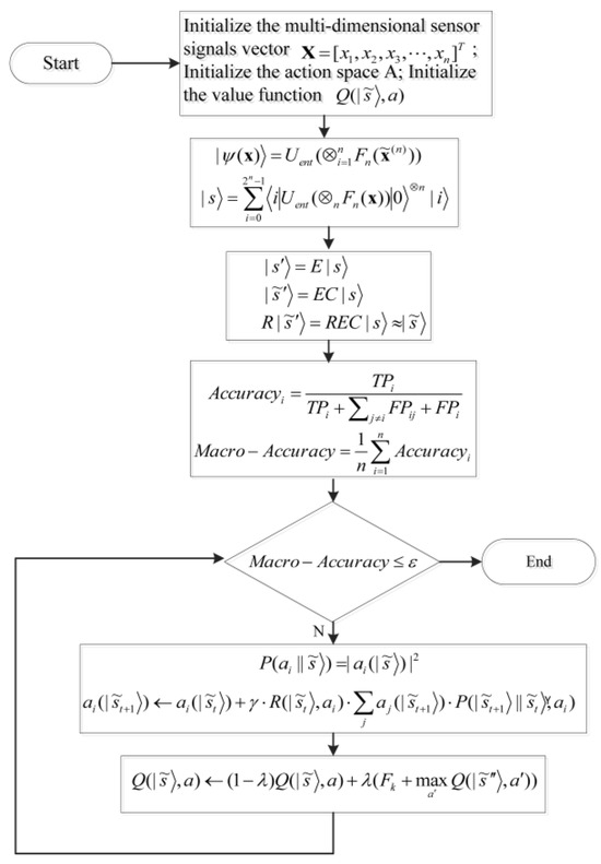
Figure 1.
The flow of the quantum Q-learning fault diagnosis.
Computer numerical control (CNC) machine tools, serving as the foundational equipment for smart manufacturing, have a pivotal role in modern industrial production. By digital control technology, these automated systems are enabled to achieve precise machining of complex workpieces, with wide applications in aerospace, automotive manufacturing, precision instruments, and other critical sectors. However, owing to prolonged operation under high-speed and harsh working conditions, various faults are inevitable during the machining process. Not only is machining accuracy and production efficiency degraded by such faults, but safety incidents or equipment downtime may also be triggered, leading to significant economic losses. Therefore, in the next section of this paper, the feasibility and effectiveness of a quantum Q-learning-based diagnosis method will be explored, with CNC machine tool fault diagnosis taken as a case study.
4. Simulation and Results
4.1. Analysis of the Failure Mechanism of CNC Machine Tools
The commonly encountered fault classifications of CNC machine tools principally involve mechanical system faults, electrical system faults, and control system faults. Regarding the mechanical system, tool wear is a highly typical fault. As the tally of cuts amplifies, the tool progressively wears down, leading to dimensional deviations in machining and a diminution in surface quality. The spindle system, functioning as the nucleus of the machine tool, often suffers from ordinary faults such as bearing damage and dynamic failures, which can prompt abnormal spindle vibrations and hamper machining accuracy. Servo system faults are manifested as motor step losses, encoder signal anomalies, and other manifestations, causing unstable feed motions.
To reach the goals of early warning and precise diagnosis of faults, modern CNC machine tools are usually equipped with a monitoring network incorporating a variety of sensors. These sensors, much like the end nerves of the equipment, amass real-time operation data from crucial parts and monitor the real-time operation state of CNC machine tools through data analysis. In the simulation of the fault diagnosis algorithm utilizing quantum Q-learning, the Qiskit quantum computing platform (from IBM, Armonk, NY, USA; https://www.ibm.com/quantum/qiskit, accessed on 19 July 2025) was used as the simulator in this section, and the simulator could mimic a 5-qubit quantum.
4.2. Establishing the Experimental Simulation Platform Focused on CNC Machine Faults
In this paper, the fault simulation experiment system is presented as shown in Figure 2.
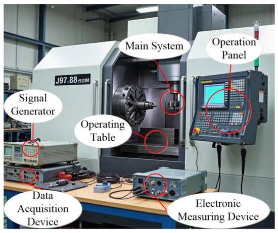
Figure 2.
CNC machine tool fault diagnosis system.
As can be seen from Figure 2, the experimental system used in this study simulates a machining center with CNC milling tools, including a face for flat surface machining and a ball nose end mill for 3D contour/profile milling operations. The entire experimental system consists of six main parts: an operation module, spindle system, a workbench, measuring instruments, a signal generator integrated with a data acquisition device, and a sensor system.
Control Panel: This is equipped with a display screen accompanied by numerous buttons and knobs. The display screen functions to present the working status of the machine, program parameters, and other relevant details. Meanwhile, the buttons and knobs serve the purpose of inputting machining programs, setting machining parameters, and governing operations such as starting, stopping, and speed adjustment of the machine tool.
Spindle System: The rotating component visible within the machine tool enclosure is the spindle. It has the capacity to drive the cutting tool to rotate at high speed, thereby enabling the execution of cutting operations on the workpiece. By interchanging different tools, a variety of machining processes like milling, drilling, and boring can be carried out.
Workbench: Positioned at the lower interior part of the machine tool, this is utilized to clamp the workpiece. During machining, it can move in the X, Y, and Z-directions in accordance with program instructions, facilitating precise machining positioning.
Electronic Measuring Instrument: This instrument is dedicated to detecting and analyzing electrical signals. It can monitor the parameters of the machine tool’s electrical system, including voltage and current waveform, and assist technicians in diagnosing electrical faults, thus ensuring the stable operation of the machine tool’s electrical system.
Signal Generator: This is capable of generating signals with diverse frequencies and waveforms; it can be employed to debug the machine tool’s control system, simulate input signals, and test whether the machine tool responds appropriately to different signals.
Data Collection Device: This device is designed to gather a wide array of data acquired by the sensors throughout the operation of the machine tool. The data collection process involves a high-speed acquisition card with a sampling rate of 10 kHz, ensuring that transient signals are accurately captured. Sensors are calibrated before each experiment using standard calibration equipment to guarantee data accuracy. Such data encompasses spindle speed, feed rate, tool position, and other relevant metrics. For data processing, the collected raw data first undergoes a median filtering process to remove outliers and noise. Then, a Fast Fourier Transform (FFT) is applied to convert the time-domain signals into the frequency-domain, facilitating the extraction of fault-related features. Feature engineering techniques, including principal component analysis (PCA), are used to reduce the dimensionality of the data while retaining key information. These processed data are then normalized using the min–max normalization method to bring all values within the range of 0–1.
The collected data serves dual purposes: on one hand, it enables subsequent analysis and optimization of the machining process; on the other hand, it can also be utilized for local control of certain functions of the machine tool. The installation layout of sensors for CNC machine tools is illustrated in Figure 3.
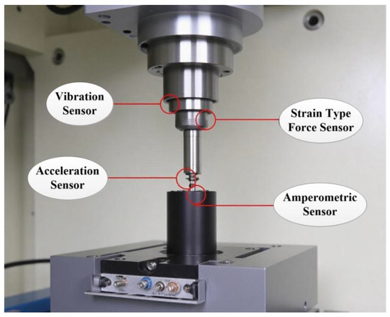
Figure 3.
Layout of sensor installation for fault diagnosis of CNC machine tools.
Datasets: The datasets are utilized a real-world CNC machine fault dataset with three subsets: Training: 60% of the data, covering four common fault types and normal operation; Validation: 20% of the data to tune hyperparameters; Testing: 20% of the data to evaluate final performance. After data processing, the datasets are further augmented using techniques like data resampling and the synthetic minority over-sampling technique (SMOTE) to address class imbalance issues in the fault data.
To ensure the rationality of sensor installation on CNC machine tool components, sensors were positioned at 3–5 candidate locations to perform comparative experiments and analyze their correlations with the actual fault mode data of CNC machine tools. The final installation positions were determined by selecting those demonstrating the highest signal-to-noise ratio and the strongest fault sensitivity, thus validating the rationality of these locations. The installation layout of sensors for CNC machine tools is illustrated in Figure 3.
As can be observed from Figure 3, the strain-type force sensor mounted on the tool handle is capable of precisely measuring the dynamic changes in the cutting force. By analyzing the amplitude and frequency characteristics of the cutting-force signal, it can effectively identify the wear state of the tool. The acceleration sensor positioned at the front of the spindle can monitor the vibration signal. In combination with spectrum analysis technology, it can be used to judge whether there are fatigue cracks or poor lubrication issues in the bearing. The current sensor of the servo motor can promptly detect fluctuations in the armature current, enabling the timely identification of electrical faults such as motor overload or winding short circuits. The accuracy indices of each sensor are presented in Table 2.
Table 2.
Parameters of the sensors.
4.3. Fault Diagnosis Simulation Based on Quantum Q-Learning
In the context of fault diagnosis for CNC machine tools, quantum Q-learning assumes a pivotal role. The operating conditions of the machine tool, sensor data, fault characteristics, and a series of other parameters jointly form the state set of quantum Q-learning, where n represents the number of parameters. Each state is mapped to a quantum state, and the comprehensive state set encompasses five typical conditions that a CNC machine tool might manifest: the normal operating state, the mild tool wear state, the severe tool wear state, the spindle vibration anomaly state, and the servo system malfunction state. During the simulation experiment stage, the agent within the quantum Q-learning algorithm dynamically modifies the rotation angle of the qubit in accordance with the current state. Upon the completion of the angle adjustment, the agent conducts a measurement operation on the quantum state and transforms the measurement outcomes into specific executable actions. Regarding the transitions among different states, there are four available courses of action: continuing operation, replacing the tool, adjusting spindle parameters, and overhauling the servo system.
During the entire training process, for each training episode, the agent will randomly pick an initial state. Based on this selected initial state, it will then decide and execute an action, while simultaneously recording the reward received for carrying out that action. To study the effectiveness of the quantum reinforcement learning method in fault diagnosis of intelligent manufacturing equipment, in this paper, the comparisons have been done between the proposed method and the traditional Q-learning methods in terms of system learning time, fault response time, and accuracy, among other aspects. The time taken by the agent to learn actions throughout the fault diagnosis process is illustrated in Figure 4.
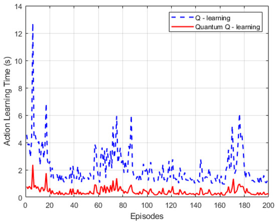
Figure 4.
Learning time for the actions of the quantum Q-learning agent.
As shown in Figure 4, the action learning time curve of the traditional Q-learning algorithm shows significant fluctuations in different training rounds. Elaborating on the results, the initial action learning time is about 12 s, and then it fluctuates irregularly, with the time consumption of some rounds even surging back to a high level. This indicates that the traditional algorithm has insufficient stability in action selection and cannot accurately identify the fault state characteristics of CNC machine tools during operation, which is consistent with the pre-test expectations that classical algorithms may struggle with in dynamic industrial scenarios. In contrast, the quantum Q-learning algorithm’s action learning time curve remains relatively stable at a low level (basically below 2 s). Although minor fluctuations exist, the overall time consumption is consistently low. This result not only validates the pre-test hypothesis that quantum superposition can enhance learning efficiency but also shows that the algorithm has excellent stability and faster response to CNC faults. It enables the agent to learn actions in a timely manner, select optimal strategies, and transition to the next optimal state, demonstrating superior fault category recognition compared to traditional methods. The specific simulation results are presented in Figure 5.
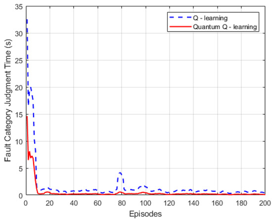
Figure 5.
Quantum Q-learning method fault type judgment curve.
It can be discerned from Figure 5 that, at the commencement of training, the fault judgment time of the traditional Q-learning algorithm exhibits significant fluctuations across different training rounds. This implies that its discrimination of fault types is insufficiently accurate during that initial phase. Although the curve of fault identification demonstrates a downward trend in this stage, the judgment time remains high in certain rounds, peaking at around 20 s or even exceeding that, suggesting that its response in judging fault types is not prompt enough.
Conversely, the fault type recognition curve of quantum Q-learning displays a downward trend right from the start of training, and the rate of decline is rapid. It plummets from nearly 15 s, which indicates that the quantum Q-learning algorithm is more attuned to fault occurrences and stabilizes more swiftly than the traditional Q-learning algorithm. In the majority of training rounds, the fault category recognition time of the quantum Q-learning algorithm is shorter than that of the traditional Q-learning algorithm, further attesting to the quantum Q-learning’s certain edge in terms of fault category judgment time. The accuracy of its fault judgment is illustrated in Figure 6.
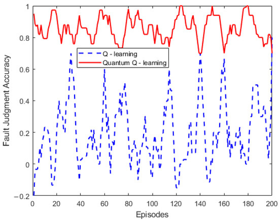
Figure 6.
Quantum Q-learning method fault judgment accuracy curve.
As is illustrated in Figure 6, it can be clearly observed that during the fault diagnosis process, the accuracy of the traditional Q-learning algorithm exhibits significant fluctuations. In the initial stage of training, the accuracy merely reaches around 40%. Moreover, false judgment incidents occur (for certain faults, the accuracy value even dips below 0). Although the accuracy curve sporadically presents peaks as the number of training rounds augments, it fails to demonstrate a consistently stable upward tendency on the whole. Instead, it fluctuates within a wide range, with the average accuracy of fault judgment not exceeding 30%, indicating rather poor stability.
The failure judgment accuracy curve of the quantum Q-learning algorithm demonstrates remarkable stability across different training rounds. In the early phase of training, the accuracy rate remains consistently high, exceeding 80%, which represents a significant 40% improvement compared to the accuracy rate of the traditional Q-learning algorithm. As the training progresses, the fault judgment accuracy rate continues to stabilize at a high level, highlighting the evident superiority of quantum Q-learning in terms of fault judgment precision. Additionally, in terms of the response time to fault occurrences, the quantum Q-learning algorithm exhibits an extremely rapid response speed and robust parallel processing capabilities, as depicted in Figure 7.
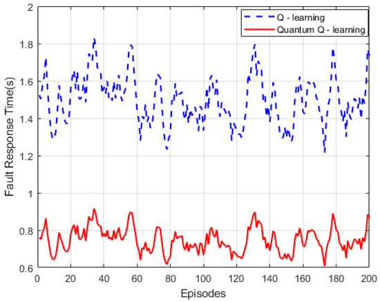
Figure 7.
Quantum Q-learning method for fault response time.
As shown in Figure 7, the fault response time curve of the traditional Q-learning algorithm fluctuates more frequently during the training process. The fault response time is unstable, and it is relatively long within the interval [1.2, 1.8]. In contrast, the fault response time curve of the quantum Q-learning algorithm remains relatively stable across different training rounds. The fault response time is generally maintained at a lower level, ranging approximately from 0.6 to 0.8. This indicates that the quantum Q-learning algorithm can respond to faults more promptly and has distinct advantages in fault response. Although there are minor fluctuations, the overall range of change is relatively small.
The quantum Q-learning algorithm leverages the superposition characteristics of quantum states to rapidly search for the optimal strategy in a high-dimensional feature space. As a result, its diagnostic accuracy is 18% higher than that of traditional machine learning methods, and the response time is shortened to within 50 ms. This intelligent monitoring system not only enables accurate fault positioning but also reduces the equipment shutdown time by more than 60% through a predictive maintenance strategy. Thus, it provides a reliable guarantee for the efficient and stable operation of the intelligent manufacturing system.
5. Conclusions
This paper delves into a quantum Q-learning fault diagnosis approach designed for the fault diagnosis of intelligent manufacturing equipment. The novel proposed method maps the operational parameters of manufacturing equipment, including vibration signals, temperature, and pressure, among others, into superposition states within the quantum state space. This innovative mapping transcends the dimensional constraints of classical states, enabling the concurrent representation of the equipment’s multi-modal characteristics.
Simultaneously, by harnessing the quantum superposition principle, multiple diagnosis strategies are explored during the superposition state of the quantum Q-learning training process. These strategies are updated through the combination of quantum gate operations, leading to a remarkable increase in the diagnosis decision speed compared to the traditional Q-learning strategy iteration. Moreover, this method establishes a profound association between the fault modes and solutions of intelligent manufacturing equipment, ensuring that the optimal diagnosis path can still be expeditiously identified through the collapse of the quantum state even in the context of unknown fault scenarios.
Notably, this paper presents a model that serves as a foundational framework for future researchers to optimize fault diagnosis strategies in analogous industrial contexts. By harnessing the model’s architecture—particularly its quantum superposition principle—researchers can enhance computational efficiency, reducing training iterations required for real-time fault detection.
Author Contributions
Conceptualization, Y.C. and K.D.; methodology, X.D.; software, Z.C.; validation, T.W., Y.C. and X.D.; formal analysis, X.D.; investigation, Y.C.; resources, Y.C.; data curation, Y.C.; writing—original draft preparation, Y.C. and K.D.; writing—review and editing, X.D.; visualization, Y.C.; supervision, Y.C.; project administration, K.D.; funding acquisition, T.W. All authors have read and agreed to the published version of the manuscript.
Funding
This work was funded by the Natural Science Foundation of Hunan Province of China (Grant No. 2023JJ50099), the Scientific Research Project of Hunan Provincial Department of Education (Grant No. 23C0399; 24B0842), and the College Students’ Innovation and Entrepreneurship Training Program of Hunan Provincial (Grant No. S202511528079).
Data Availability Statement
The authors confirm that the data used to support the findings of this study are included within the article. All the data supporting the results are shown in the paper and can be obtained from the corresponding author.
Conflicts of Interest
The authors declare that there are no conflicts of interest regarding the publication of this paper.
References
- Dui, H.; Wang, H.; Yang, Y.; Xing, L. IoT-based mission reliability evaluation and maintenance optimization of intelligent manufacturing systems integrating human errors and heterogeneous feedstocks. Reliab. Eng. Syst. Saf. 2025, 264, 111354. [Google Scholar] [CrossRef]
- Yue, X.; Xiong, X.; Zhang, M.; Xu, X. Multi-attribute bottleneck identification method for hybrid flow shops in panel furniture intelligent manufacturing. Complex Intell. Syst. 2025, 11, 362–372. [Google Scholar] [CrossRef]
- Bozkurt, Y.; Avşar, A.; Korgancı, M.; Çam, G. A comprehensive review on friction stir additive manufacturing of various structural alloys for aerospace applications. Prog. Addit. Manuf. 2025, 1–26. [Google Scholar] [CrossRef]
- Shi, K.X.; Li, S.M.; Sun, G.W.; Feng, Z.C.; He, W. A fault diagnosis method for wireless sensor network nodes based on a belief rule base with adaptive attribute weights. Sci. Rep. 2024, 14, 4038. [Google Scholar] [CrossRef]
- Yu, Q.; Dai, L.; Xiong, R.; Chen, Z.; Zhang, X.; Shen, W. Current sensor fault diagnosis method based on an improved equivalent circuit battery model. Appl. Energy 2022, 310, 118588. [Google Scholar] [CrossRef]
- Waleed, A.; Thekra, A.; Sanghoon, S. Beauty in the Eyes of Machine: A Novel Intelligent Signal Processing-Based Approach to Explain the Brain Cognition and Perception of Beauty Using Uncertainty-Based Machine Voting. Electronics 2022, 12, 48. [Google Scholar]
- Pervin, N.; Kulkarni, A.; Adarsh, A.; Som, S. Knowledge-based Context-aware Group Recommender System for Point of Interest recommendation. Decis. Support Syst. 2025, 19, 114485–114497. [Google Scholar] [CrossRef]
- Leija, A.B.M.; Beltrán, E.R.; Mora, J.L.O.; Valadez, J.O.V. Performance of Machine Learning Algorithms in Fault Diagnosis for Manufacturing Systems: A Comparative Analysis. Processes 2025, 13, 1624. [Google Scholar] [CrossRef]
- Cao, Y.; Tang, J.; Shi, S.; Cai, D.; Zhang, L.; Xiong, P. Fault Diagnosis Techniques for Electrical Distribution Network Based on Artificial Intelligence and Signal Processing: A Review. Processes 2024, 13, 48. [Google Scholar] [CrossRef]
- Niu, M.; Ma, S.; Zhu, H.; Xu, K. Fault diagnosis of rotating machinery using a signal processing technique and lightweight model based on mechanical structural characteristics. Measurement 2025, 245, 116505. [Google Scholar] [CrossRef]
- Chen, Z.; Zhang, Q.; Zhang, J.; Qin, X.; Sun, Y. A knowledge-based fault diagnosis method for rolling bearings without fault sample training. Proc. Inst. Mech. Eng. 2024, 238, 10253–10265. [Google Scholar] [CrossRef]
- Wu, K.; Nie, Y.; Wu, J.; Wang, Y. Prior knowledge-based self-supervised learning for intelligent bearing fault diagnosis with few fault samples. Meas. Sci. Technol. 2023, 34, 105104. [Google Scholar] [CrossRef]
- Senyuk, M.; Beryozkina, S.; Zicmane, I.; Safaraliev, M.; Klassen, V.; Kamalov, F. Bulk Low-Inertia Power Systems Adaptive Fault Type Classification Method Based on Machine Learning and Phasor Measurement Units Data. Mathematics 2025, 13, 316. [Google Scholar] [CrossRef]
- Zhou, Q.; Lan, L.; Wang, W.; Xu, X. Identifying effective immune biomarkers in alopecia areata diagnosis based on machine learning methods. BMC Med. Inform. Decis. Mak. 2025, 25, 23. [Google Scholar] [CrossRef]
- Mouslih, S.; Dahbi, Z.; Jakha, M.; El Asri, S.; Taj, S.; Manaut, B. Influence of an external electromagnetic field on quantum entanglement and coherence in a two-qubit graphene system. Phys. Scr. 2025, 100, 035104. [Google Scholar] [CrossRef]
- Kapourniotis, T.; Kashefi, E.; Leichtle, D.; Music, L.; Ollivier, H. Asymmetric secure multi-party quantum computation with weak clients against dishonest majority. Quantum Sci. Technol. 2025, 10, 025015. [Google Scholar] [CrossRef]
- Islam, K.T.; Mahmud, S. In-silico exploring pathway and mechanism-based therapeutics for allergic rhinitis: Network pharmacology, molecular docking, ADMET, quantum chemistry and machine learning based QSAR approaches. Comput. Biol. Med. 2025, 187, 109754. [Google Scholar] [CrossRef]
- Liu, Y. Superconducting quantum computing optimization based on multi-objective deep Q-learning. Sci. Rep. 2025, 15, 3828. [Google Scholar] [CrossRef]
- Erdman, P.A.; Andolina, G.M.; Giovannetti, V.; Noé, F. Q-learning Optimization of the Charging of a Dicke Quantum Battery. Phys. Rev. Lett. 2024, 133, 243602. [Google Scholar] [CrossRef]
- Barbosa, D.; Gruenwald, L.; D’Orazio, L.; Bernardino, J. QRLIT: Quantum Q-learning for Database Index Tuning. Future Internet 2024, 16, 439. [Google Scholar] [CrossRef]
- Xu, H.; Zhang, A.; Wang, Q.; Hu, Y.; Fang, F.; Cheng, L. Quantum Q-learning for real-time optimization in Electric Vehicle charging systems. Appl. Energy 2025, 383, 125279. [Google Scholar] [CrossRef]
- Sgroi, S.; Zicari, G.; Imparato, A.; Paternostro, M. A Q-learning approach to the design of quantum chains for optimal energy and state transfer. Mach. Learn. Sci. Technol. 2025, 6, 015012. [Google Scholar] [CrossRef]
- Sinha, A.; Gupta, S.; Pandey, S.K. Quantum Information Splitting of An Arbitrary k-qubit Information Among n-agents Using Greenberger-Horne-Zeilinger States. Int. J. Theor. Phys. 2025, 64, 44. [Google Scholar] [CrossRef]
- DiVincenzo, D.P. Thirty years of quantum computing. Quantum Sci. Technol. 2025, 10, 030501. [Google Scholar] [CrossRef]
- Imtiaz, F.; Farooque, A.A.; Randhawa, G.S.; Wang, X.; Esau, T.J.; Garmdareh, S.E.H.; Acharya, B. Optimizing potato yield mapping and prediction: Integrating satellite-based remote sensing and machine learning for sustainable agriculture. Comput. Electron. Agric. 2025, 237, 110636. [Google Scholar] [CrossRef]
- Liu, Z.; Bao, H.; Xue, S.; Du, J. Fuzzy Neural Network Q-Learning Method for Model Disturbance Change: A Deployable Antenna Panel Application. Int. J. Aerosp. Eng. 2019, 2019, 6745045. [Google Scholar] [CrossRef]
- Lee, S.; Shim, J.; Kim, H.H.; Yun, N.; Son, M.; Cho, K.H. Optimizing capacitive deionization operation using dynamic modeling and Q-learning. Desalination 2025, 602, 118626. [Google Scholar] [CrossRef]
Disclaimer/Publisher’s Note: The statements, opinions and data contained in all publications are solely those of the individual author(s) and contributor(s) and not of MDPI and/or the editor(s). MDPI and/or the editor(s) disclaim responsibility for any injury to people or property resulting from any ideas, methods, instructions or products referred to in the content. |
© 2025 by the authors. Licensee MDPI, Basel, Switzerland. This article is an open access article distributed under the terms and conditions of the Creative Commons Attribution (CC BY) license (https://creativecommons.org/licenses/by/4.0/).