Abstract
Model validation is an essential part of CFD-based projects. Despite being successfully employed for decades, the level and extent of CFD model validation details vary significantly in the published literature, which, in turn, adversely affects the repeatability and usefulness of published models and data. This study explores the various challenges associated with validating CFD models of thermodynamic components, namely, the compressors and their performance evaluation. The methodology involves blade generation through TurboGrid and BladeGen, mesh generation to ensure computational efficiency, and pre-processing with CFX to define boundary conditions and turbulence models, all within ANSYS 2024 R1. Three case studies are discussed, each assessing different compressor configurations and common challenges encountered during the model validation stage. Based on the case studies, a number of recommendations are presented relating to best practices in terms of both the use of published materials to validate new models and the level of detail required for experimental or simulation publication to ensure they can be replicated or used to validate a new model.
1. Introduction
Computational Fluid Dynamics (CFD) has become indispensable in the design, analysis, and optimisation of thermofluid systems, with its accuracy and reliability largely contingent upon rigorous model validation. This is most common in turbomachinery applications such as compressors and turbines, where CFD is used to resolve complex internal flows under high-pressure, high-speed configurations [1,2]. In such systems, geometric complexity, three-dimensional unsteadiness, and strong shock–boundary layer interactions pose significant modelling challenges that necessitate robust and well-verified numerical approaches [3,4].
However, as highlighted in the literature, the reproducibility and replicability of CFD studies remain inconsistent, impeding the utility and generalisability of published results [5,6]. Despite an abundance of validation case studies, discrepancies in geometric fidelity, meshing strategy, and solver configuration often result in deviations between nominally similar studies, raising concerns over the robustness of simulation frameworks [7,8]. Even when code, mesh, and solver settings are openly shared, results may diverge due to undocumented dependencies, inconsistent software environments, or small implementation differences that propagate over thousands of time steps. Recent studies underscore the critical importance of transparent documentation and standardised workflows, especially when comparing simulation outputs with experimental benchmarks or legacy computational data [9]. These concerns are evident in compressor modelling, where small changes in mesh topology, turbulence modelling, or blade definition can significantly alter predicted performance metrics [10]. Furthermore, modern investigations have shown that turbulence model selection, averaging methods, and mesh distribution near regions of tip clearance or hub corner stall can lead to substantial variations in flow predictions, particularly near stall onset [11].
Over time, expectations surrounding CFD verification and validation have evolved. Mikulec and Piehl [12] show that modern validation efforts increasingly rely on detailed documentation of simulation setups, including mesh and time-step sensitivity studies, with grid convergence quantified using tools like the Grid Convergence Index. Their work demonstrated close agreement between RANS-based full-scale ship simulations and corrected sea trial data, reinforcing the need for transparent workflows and clearly defined validation criteria. This shift in validation practice reflects both the increased complexity of CFD applications and their growing role in engineering design and compliance. As simulation capability has advanced, so too have the requirements for reproducibility and verification, particularly where CFD informs critical decisions [13].
A review of the recent literature shows a consistent reliance on a set of key validation parameters to assess the accuracy and performance of compressor simulations. One of the most widespread approaches is the use of pressure ratio agreement, wherein experimentally derived static or total pressures at various stations and through the compressor—typically across the diffuser or rotor-stator interface—are compared directly with CFD predictions. Dewar et al. validated a centrifugal compressor using this method and reported less than 2% deviations at design point and up to 5% at off-design points, highlighting the capacity of CFD for capturing global thermodynamic behaviour with reasonable accuracy [14]. Mass flow rate and power consumption are essential parameters for global validation, especially in the case of scroll or reciprocating compressors, where internal leakage and mechanical losses need to be considered [15]. Furthermore, at a finer level, velocity profiles within impeller passages and diffusers are employed to evaluate local flow structures, such as secondary flows and separation zones; yet, such an assessment is typically reliant on the availability of high-resolution experimental data.
In addition to straightforward physical comparisons, a number of studies advocate for the application of statistical or error-based measures. Hora et al. categorise several error-based validation techniques, encompassing relative and absolute error norms [16]. Rasmussen et al. propose a robust comparison of uncertainty quantification metrics—such as Spearman’s rank correlation, negative log-likelihood, and miscalibration area—ultimately recommending error-based calibration as the most reliable metric for assessing prediction accuracy and uncertainty alignment [17]. Kat et al. also suggest a relative error-based approach, particularly for periodic time series data, to enable direct comparison between transient simulation and experimental measurement [18]. These findings collectively indicate that the choice of validation metrics needs to be guided by the compressor type, operating range, and available measurement data, with an increasing focus on both global performance reconciliation and local flow feature verification.
This paper explores a methodology for validating CFD models of rotating turbomachinery components, specifically axial and radial compressors, using TurboGrid and CFX, within ANSYS 2024 R1. Three case studies are examined, each involving the reconstruction of compressor geometries from the original datasets or technical drawings, followed by structured mesh generation and solver configuration. The aim is to replicate key performance metrics as reported in the respective reference studies. In doing so, the research evaluates the extent to which published information supports accurate model replication, highlighting practical challenges and limitations in current validation workflows. The findings are used to inform a set of best-practice recommendations, with particular emphasis on reproducibility and methodological transparency.
The primary objective of the paper is to demonstrate that the reporting of CFD analyses of compressors in current literature often lacks the necessary detail to enable effective validation or reproduction of results. In this context, it is important to distinguish between replicability—achieving the same results using the same setup—and reproducibility—obtaining comparable results using different tools or methods. By attempting to replicate the findings of three published case studies using only the information provided therein, this work illustrates how inconsistencies or omissions in documented methods can undermine confidence in CFD-based studies. The outcomes serve as a foundation for recommending improved standards in the reporting of CFD simulations, with the goal of enhancing the reliability, reproducibility, and utility of future research in compressor modelling.
2. Methodology
The following are case studies of the multi-stage procedure of component performance analysis with ANSYS 2024 R1 software. The output was achieved with three critical stages: importing the given model file, meshing with ANSYS TurboGrid, and pre-processing and simulation with ANSYS CFX. These case studies were selected with care so that they represented a clear range of settings and geometries. The three cases were as follows:
- Case 1: Experimental and Computational Analysis of a Transonic Compressor Rotor [19].
- Case 2: Validation of a CFD Model of a Single Stage Centrifugal Compressor by Local Flow Parameters [20].
- Case 3: Multidisciplinary optimisation of the SRV2-O radial compressor using an adjoint-based approach [21].
The aim of this study is to address challenges involved in duplicating simulation data outlined in case studies and compare them with experimental data mentioned in each paper. Although each of the case studies has fairly distinct objectives and conclusions, this study aimed at finding obstacles and universal problems with validating the ANSYS 2024 solver with known simulation and experimental data. All sections used data from the respective papers where possible. When this was not feasible, either due to a lack of data or software constraints, the context of the paper was used to provide the most accurate form of simulation.
Although the specific details of each simulation are dependent on the conditions specified in each of the case studies, the general approach to the simulation follows that in [14]. In [14] CFD simulations were performed using ANSYS CFX and directly compared to experimental measurements. The simulation results were validated against the measurements, in terms of the measured and simulated pressures, at the tapping points on the experimental compressor for a range of mass flow rates and rotational speeds. The results showed that away from the tip, there was a discrepancy of less than 2 % at the design operating point, which increased to just over 5% further from this point. Closer to the top, the discrepancies were slightly larger, but no more than 8%. This provides validation of the general approach taken in the present study, as set out below.
2.1. Geometry Creation
For all three case study examples, the blade geometries were created from supplied data or reconstructed from technical drawings, ensuring they matched the specifications in each reference study. These geometries were built or adapted using ANSYS TurboGrid or BladeGen, following consistent units and blade parameter conventions wherever possible.
In Case Study 1, the geometry files came from GrabCAD, including blade profiles and hub/shroud contours in the curve format. These files, which were part of a well-recognised validation study [22], were loaded into TurboGrid, and all necessary parameters were set using the geometry tab. The unit system was set to centimetres to match the reference, and the number of rotor blades was fixed at 36, as specified in the source. Blade profiles were detailed at 10% span intervals, allowing for precise reconstruction of the axial rotor’s 3D shape.
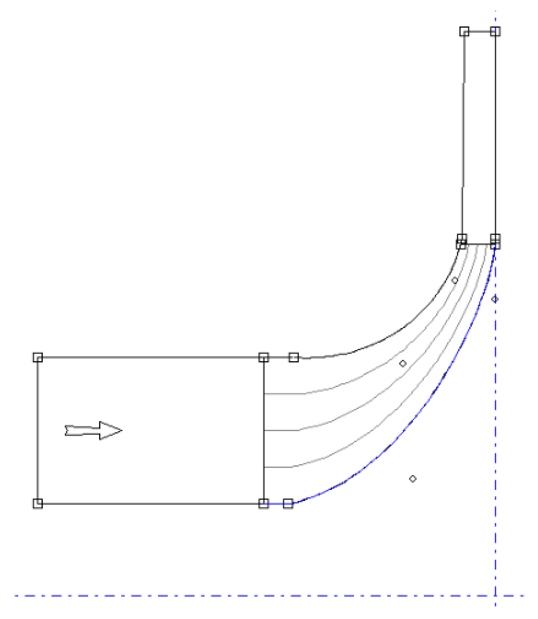
For Case Study 2, the rotor geometry was recreated using BladeGen based on a technical drawing from the reference study. Inconsistencies in radii and other dimensions were found and corrected to ensure the shape was accurate. The completed meridional curve used in the model appears in Figure 1. In BladeGen, blade angles and thickness were defined graphically—27° for the external inlet angle () and 90° for the outlet angle (). Blade thickness was set at 3.5 mm at the hub and 3 mm at the shroud, with rounded leading and trailing edges sized at half the respective thickness. Since the original paper did not mention the blade count, a manual check determined there were 20 blades.
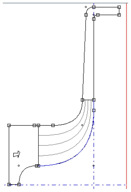
Figure 1.
Case Study 2: Created geometry.
In Case Study 3, BladeGen was again used. The meridional curve was based on a technical drawing with plotted data points, but because it lacked raw numbers, an online tool was used to extract the data digitally. The digitised points were compiled and used to build the geometry in BladeGen. The final shape is shown in Figure 2. Both main blades and splitter blades were modelled using the same approach, and the blade count was confirmed to be 13.
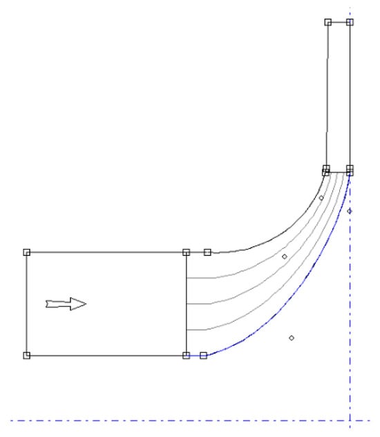
Figure 2.
Case Study 3: Created geometry.
2.2. Mesh Generation
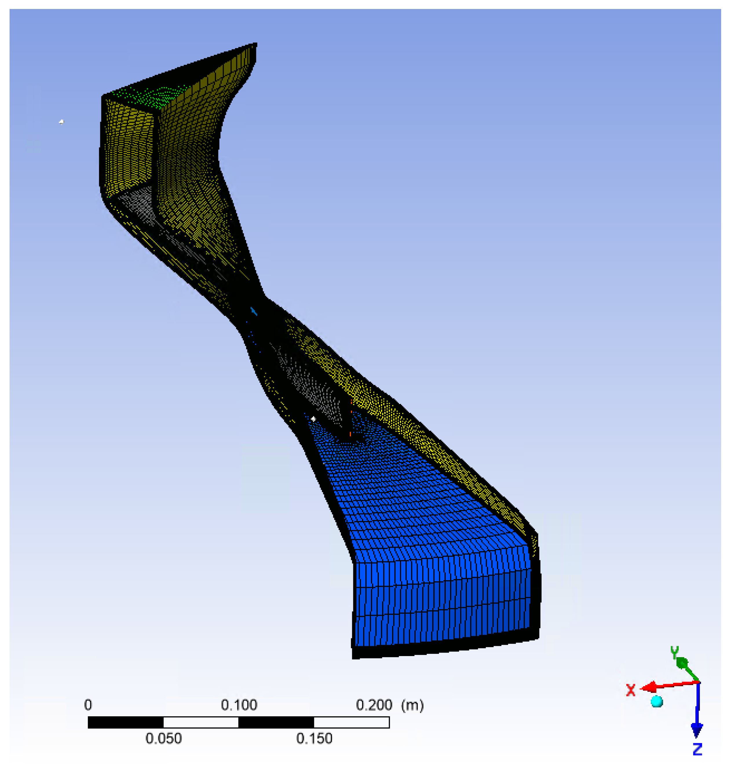
In Case Study 1, the mesh was created in TurboGrid, where the geometry was split into three separate sections to allow for targeted refinement. While the reference study did not detail the meshing method, this case used the Automatic Topology and Meshing (ATM) technique. A global size factor of 2.37 was chosen after several test runs to match the desired mesh size range. Boundary layers were refined using a proportional method based on mesh size, with a factor of 3. A constant offset was set for the first mesh element, and a maximum element growth rate of 1.2 was used to maintain mesh quality. Element sizes near walls were specified in absolute terms to enhance resolution. The final mesh included 778,386 elements and 817,168 nodes—very close to the reference values of 816,638 elements and 856,112 nodes. The mesh generated for Case Study 1 is shown in Figure 3, displaying the typical structure of a mesh for an axial rotor.

Figure 3.
Case Study 1: Generated mesh of an axial rotor.
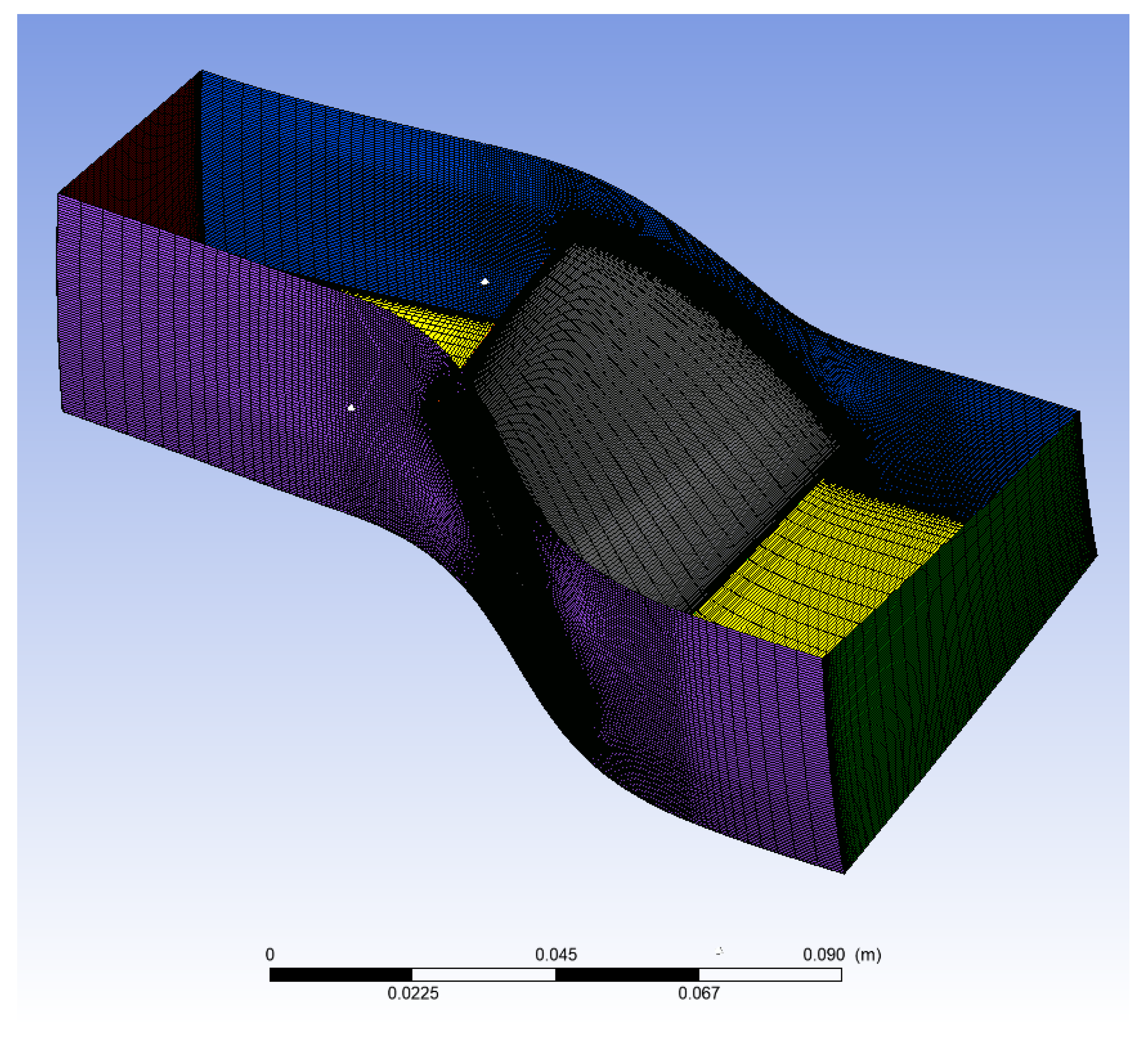
In Case Study 2, TurboGrid was also used. The mesh tab again divided the geometry into three independently adjustable regions. The original paper did not provide details about its meshing technique, but the ATM method was applied here for structured refinement. A global size factor of 2.3 was used, and boundary layer refinement followed the same proportional approach as in Case Study 1, with a base factor of 3. A constant first element offset was set, and a 1.2 expansion rate was applied to manage element transition. The total mesh included 474,192 elements and 507,452 nodes, which was lower than the 540,000 elements in the original study due to limitations in computing resources and differing meshing strategies. The generated mesh for Case Study 2 can be seen in Figure 4, which gives a good example of what a structured mesh looks like for a centrifugal compressor.

Figure 4.
Case Study 2: Generated mesh of a centrifugal compressor.
For Case Study 3, the meshing was again performed in TurboGrid, but this time the case study used the ATM method rather than the unstructured tetrahedral approach from the reference study. The original method started by meshing the CAD model’s edges, then faces, and finally the volume using Delaunay triangulation. In contrast, the ATM method in the case study provided a more even element distribution. A global size factor of 1 was used, and boundary layer refinement followed the same mesh-proportional strategy with a factor base of 3. The final mesh had 381,612 elements and 415,820 nodes, compared to the reference’s 280,000 elements and 420,000 nodes—highlighting differences in meshing approaches and computational constraints.
2.3. Solver Settings
Table 1 outlines the solver settings that were consistently used across all three replicated case studies. While the reference studies often dealt with transonic flows, the simulations presented here were run in subsonic conditions, based on how their boundaries and flow properties were defined. Each model was divided into three separate domains—Inlet, Passage Main, and Outlet—to clearly differentiate between stationary and rotating flow areas. To simulate the interaction between rotating and stationary parts, Frozen Rotor interfaces were used, assuming steady-state behaviour. Rotational periodicity was enforced at the circumferential boundaries to maintain symmetry and improve computational efficiency.

Table 1.
Common solver settings used across all case studies.
All solid surfaces—such as blades, hubs, and shrouds—were treated as no-slip walls. Air was modelled as an ideal gas in all simulations, with energy transport handled through the total energy approach. The solver setup was standardised using a high-resolution advection scheme, first-order turbulence models, and conservative automatic timescale settings. These shared configurations ensured a consistent computational framework, making it easier to compare how changes in turbulence models, rotation speeds, or flow rates affected each case. The timescale factor was adjusted individually for each simulation following an iterative process aimed at balancing convergence criteria with computational efficiency.
2.3.1. Simulation 1
In Case Study 1, the domain interfaces were handled using the Frozen Rotor model to simulate steady-state interactions between the rotor and stator. To mirror the symmetry of flow within the annular passage, rotational periodicity was applied along the circumferential boundaries. Air was treated as an ideal gas, and energy transport was governed by the total energy model. The simulation used the SST (Shear Stress Transport) turbulence model with automatic wall functions in ANSYS CFX, which closely resembles the “All y+ wall treatment” used in the STAR-CCM+ environment cited in the reference.
A mass flow inlet was applied, with the total flow rate set to 20.5196 kg/s across all sectors—this matched the near-peak efficiency operating point on the Rotor 37 curve. Turbulence intensity at the inlet was set at 3%, the same as in the reference study. Flow direction at the inlet was defined as normal to the boundary. At the outlet, a static pressure condition was used, calculated to match the desired pressure ratio of 2.084. This setup contrasts with the reference configuration, which typically used a stagnation inlet and adjusted the outlet pressure to reach the target mass flow. The change was made to match the pressure ratio values in the original study. Even though the setup was reversed, both approaches aim to recreate the same physical conditions inside the rotor passage. A full breakdown of simulation settings and physical models can be found in Table 2.
Table 2.
Case-specific solver settings for Simulation 1.
- Comparison to Reference Study
The reference study used a different set of boundary conditions and domain assumptions, most notably applying a stagnation inlet and adjusting outlet pressure to match the target mass flow. In contrast, Case Study 1 specified the mass flow directly and used a static pressure outlet. Additional differences include the explicit use of Frozen Rotor interfaces, rotational periodicity, and well-defined solver controls. A summary of the most significant changes is shown in Table 3.
Table 3.
Key differences between reference study and Case Study 1.
2.3.2. Simulation 2
In Case Study 2, the simulation setup was built in ANSYS CFX-Pre using geometry imported from TurboGrid. The model consisted of three separate fluid domains—Inlet, Passage Main, and Outlet—which were connected using general interfaces. To simulate the rotor–stator interaction under steady-state conditions, the Frozen Rotor method was applied at the boundaries between rotating and stationary sections. Rotational periodicity was also applied around the circumferential edges to reflect the symmetry of the annular flow and reduce computational demands.
The working fluid was treated as air, using the ideal gas assumption. Heat transfer was handled using the total energy model. Wall functions were automatically managed by CFX to ensure accurate resolution near solid boundaries, depending on mesh quality.
A mass flow condition was set at the inlet, with a flow rate of 7.16 kg/s and a turbulence intensity of 3%—the same conditions recorded at the Rotor 37 test inlet. Flow direction was specified as normal to the boundary. At the outlet, a static pressure condition was applied, calculated based on the target pressure ratio to match the reference performance data. All solid surfaces, including blades, hub, and shroud, were treated as no-slip walls. A full summary of domain and solver settings is shown in Table 4.
Table 4.
Case-specific solver settings for Case Study 2.
- Comparison to Reference Study
The reference study utilised stagnation inlet conditions and adjusted outlet pressure iteratively to achieve a target mass flow. In contrast, Case Study 2 specified the mass flow at the inlet and applied a static pressure at the outlet. Additionally, a different turbulence model was used (k- instead of SST), and solver control settings were explicitly defined in CFX-Pre. These distinctions are summarised in Table 5.
Table 5.
Key differences between reference study and Case Study 2.
2.3.3. Simulation 3
This simulation followed the same three-domain setup as the previous case studies, with distinct regions for the Inlet, Passage Main, and Outlet. These domains were connected using general interfaces, and the Frozen Rotor model was applied at the boundaries between rotating and stationary areas to simulate their interaction under steady-state conditions. Rotational periodicity was also enforced around the circumferential boundaries to replicate symmetry and help keep computation times efficient.
Air was used as the working fluid, modelled as an ideal gas. The Shear Stress Transport (SST) turbulence model was chosen because of its strong performance in handling adverse pressure gradients and boundary layer separation. Heat transfer was managed using the total energy model, while wall functions were automatically applied by CFX to adjust for the local mesh quality.
A mass flow condition was applied at the inlet, with the flow rate set to match the target operating point from the reference compressor. Turbulence intensity at the inlet was fixed at 3%, and flow was directed normal to the boundary. At the outlet, a static pressure boundary condition was applied, based on the pressure ratio associated with the desired operating condition. All solid components—including the impeller blades, hub, and shroud—were treated as no-slip walls. A detailed summary of the simulation and solver settings can be found in Table 6.
Table 6.
Case-specific solver settings for Case Study 3.
- Comparison to Reference Study
Simulation 3 maintained the same domain structure and general physical setup as the reference study, including the use of a mass flow inlet and a static pressure outlet. However, unlike the original setup, which applied stagnation inlet conditions and adjusted outlet pressure to match flow, this case directly prescribed the inlet flow rate. The turbulence model (SST) and interface handling (Frozen Rotor) remained consistent with the reference, but solver settings and convergence controls were explicitly defined. These distinctions are outlined in Table 7.
Table 7.
Key differences between reference study and Case Study 3.
3. Results
3.1. Case Study 1
The simulation results for Case Study 1 were examined under two key operating conditions: near-stall and peak efficiency. Important global performance indicators—including polytropic and isentropic efficiencies, the total temperature ratio (TTR), total pressure ratio (TPR), and mass flow rate (MFR)—are summarised in Table 8.
Table 8.
Global performance metrics for Case Study 1 at near-stall and peak-efficiency conditions.
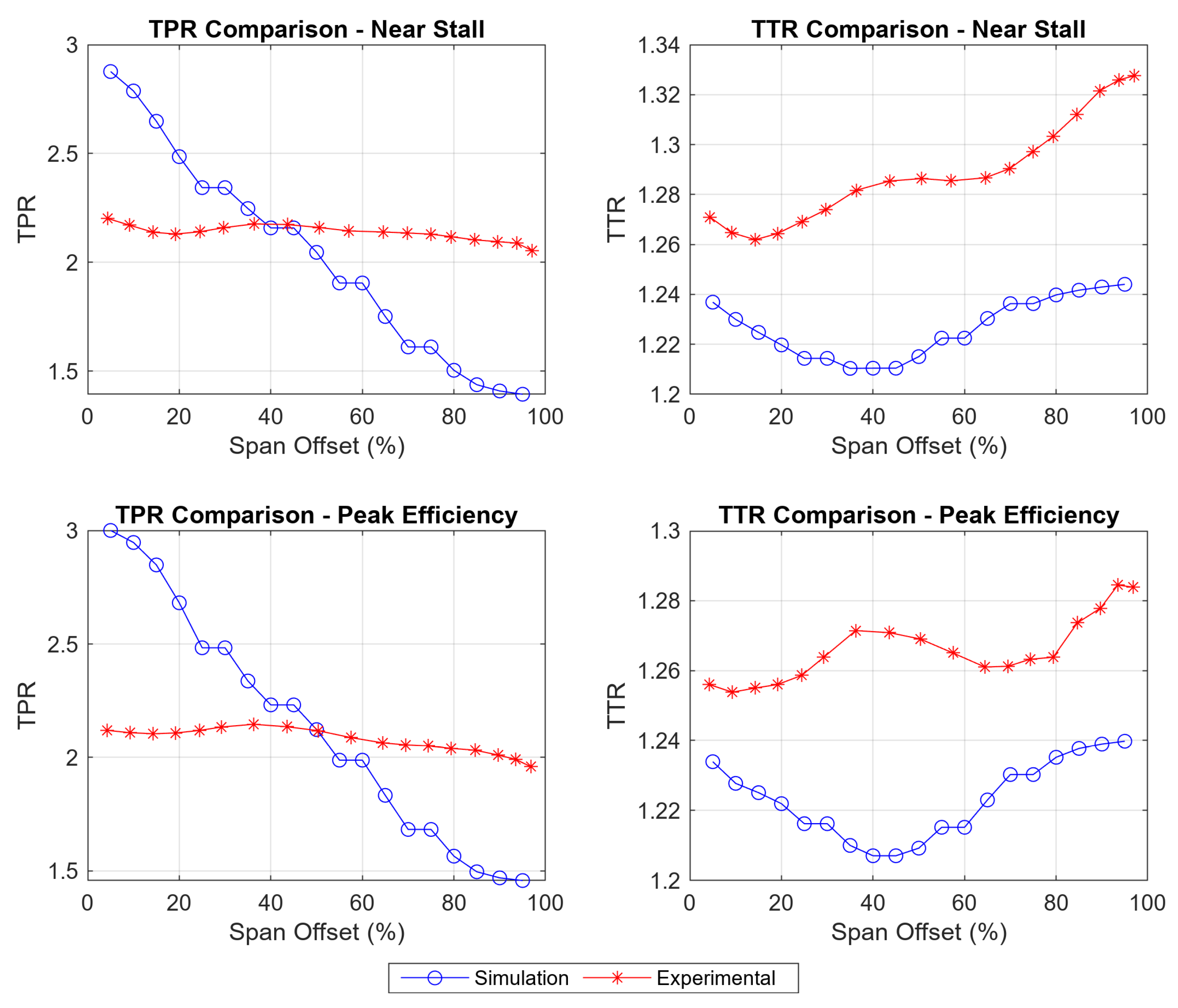
Beyond the point-based performance values, the team also looked at how TPR and TTR changed across the blade span. These spanwise distributions were measured at various radial positions, ranging from 5% to 95% of the blade height, and then compared to experimental results from the original reference study, as illustrated in Figure 5.
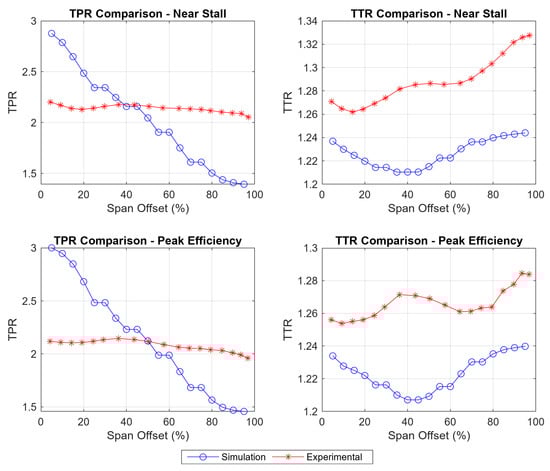
Figure 5.
Spanwise comparison of total pressure ratio (TPR) and total temperature ratio (TTR) between simulation (blue circles) and experimental data (red crosses) at near-stall (top row) and peak-efficiency (bottom row) operating points.
In both operating conditions, the TPR from the simulation showed a roughly linear drop along the span, starting from almost 3 at the hub and decreasing to about 1.4 near stall and 1.25 at peak efficiency. This trend differed from the reference study [19], which reported TPR values that stayed nearly constant along the span at just over 2. For TTR, the simulation consistently predicted lower values than those in the reference data under near-stall conditions. A similar trend was seen at peak efficiency, although the results aligned more closely near the blade tip.
3.2. Case Study 2: Off-Design Performance Evaluation
To test how the model performs under off-design conditions, simulations were run at several different mass flow rates and at two rotational speeds: 18,000 RPM and 16,000 RPM. The goal was to replicate the pressure ratio trends from the reference study and assess how much the simulated values differed.
The outcomes of these simulations are shown in Table 9 and Table 10, which detail the calculated pressure ratios and how much they deviate—expressed as percentages—from both experimental results and previously published simulation data.
Table 9.
Case Study 2 results at 18,000 RPM: Pressure ratio and deviation metrics.
Table 10.
Case Study 2 results at 16,000 RPM: Pressure ratio and deviation metrics.
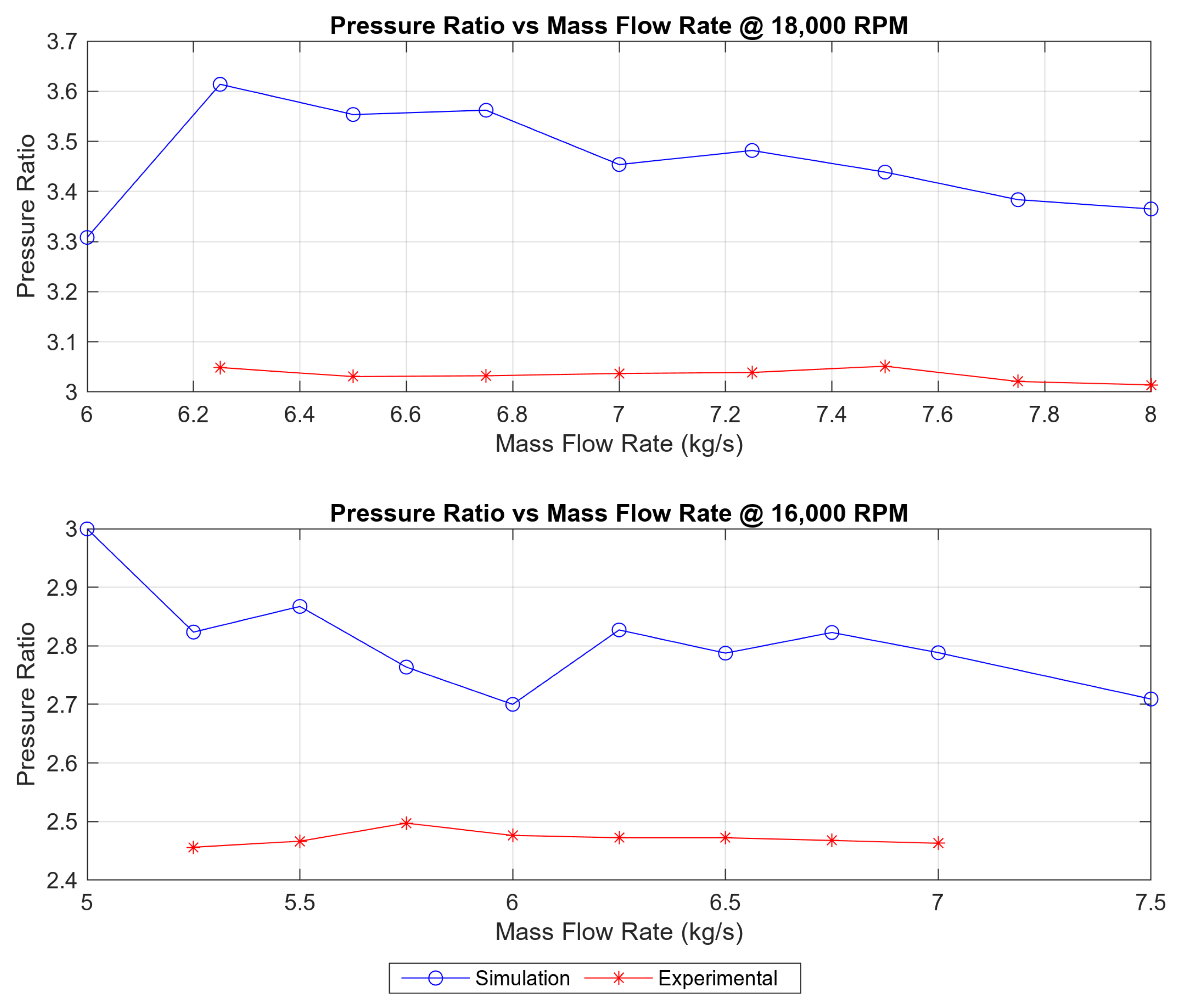
As shown in Figure 6, the simulations successfully captured the overall trend: pressure ratio increased as flow rate decreased. However, the actual pressure ratio values from the simulations were consistently higher than the experimental results, especially at the lower flow rates. Even so, the shape and slope of the simulation curves closely matched those from the reference compressor map, indicating that the model, while not perfect numerically, was still accurate in a qualitative sense.
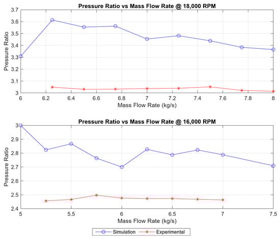
Figure 6.
Comparison of simulated and reference pressure ratio curves at 16,000 and 18,000 RPM. Solid lines indicate experimental reference data; dotted lines and markers show simulation results.
3.3. Case Study 3: Performance Evaluation of a Radial Compressor at Variable Operating Conditions
In Case Study 3, a high-speed radial compressor was tested across a range of mass flow rates, all at a fixed rotational speed of 40,000 RPM and 50,000 RPM. The aim was to see how efficiency metrics changed with varying flow rates and to compare these simulation results with the reference data.
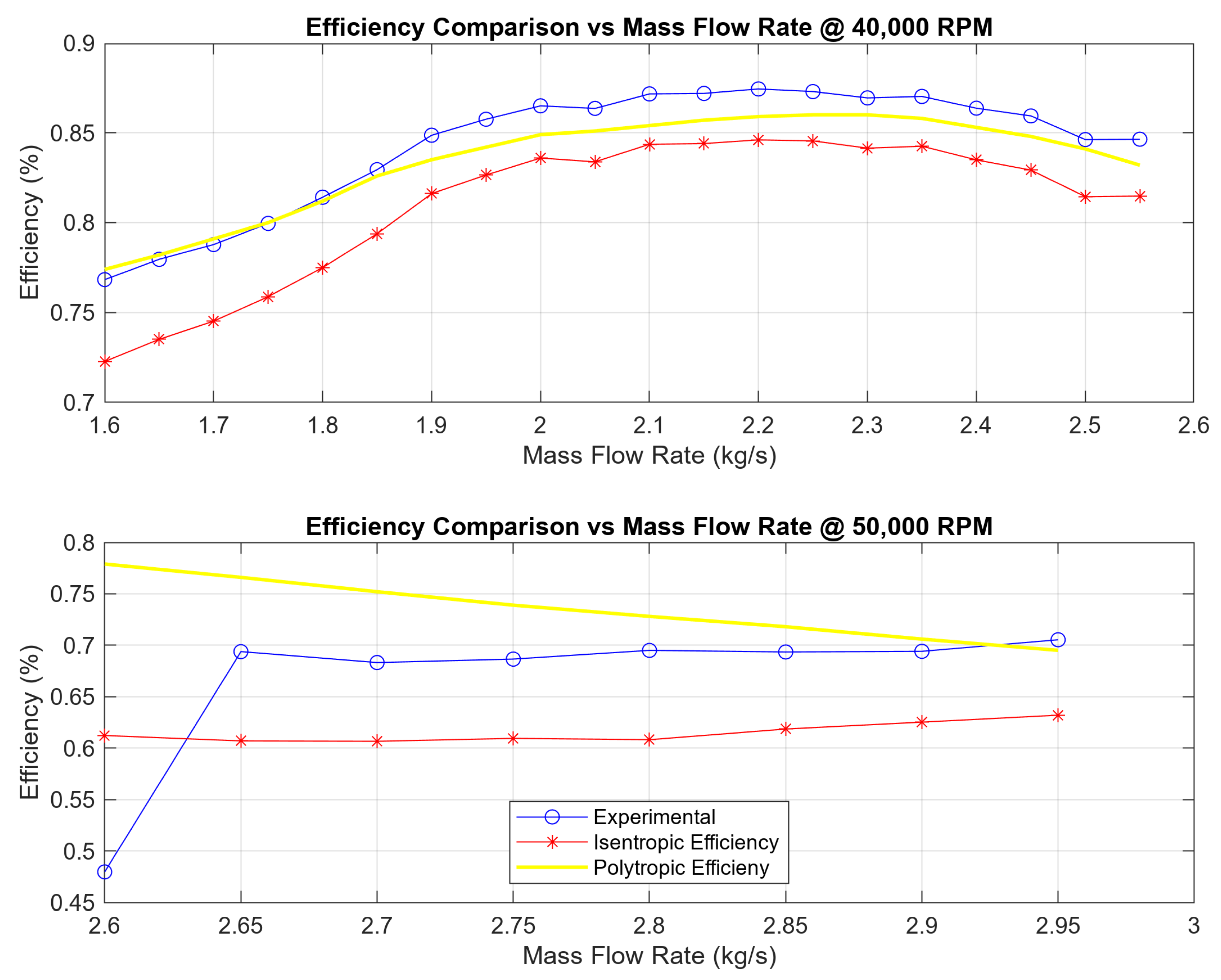
At 40,000 RPM, the simulation results showed strong alignment with reference performance data. Both polytropic and isentropic efficiency trends exhibited well-defined peaks near 2.1 kg/s, with maximum values reaching approximately 0.87 and 0.84, respectively. The predicted pressure ratio curve closely followed the expected trajectory, suggesting accurate modelling under moderate-speed operation.
At 50,000 RPM, the simulated isentropic and polytropic efficiencies deviate significantly from the expected performance profile observed at lower speeds. Both polytropic and isentropic efficiencies appear to plateau at a lower maximum value and show increased scatter across the mass flow range. Notably, these simulated trends diverge from the reference case’s total-to-total efficiency, which still maintains a smoother and more parabolic behaviour even at higher speeds.
The performance trends for both operating speeds are illustrated in Figure 7, which shows the variation of polytropic and isentropic efficiencies as a function of mass flow rate.
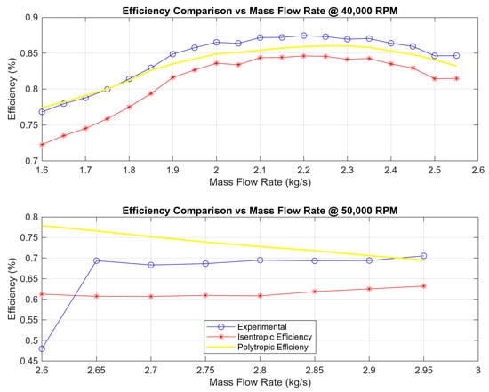
Figure 7.
Comparison of simulated polytropic and isentropic efficiencies with experimental total-to-total efficiency values across mass flow rates at 40 k and 50 k RPM.
4. Discussion
The findings presented in the three case studies were assessed against a defined convergence framework of criteria, chosen to provide accuracy in simulations, numerical stability, and agreement with reference data available. The framework entailed residual convergence below , mass imbalance maintained within ±5% for all domains, stability of critical monitoring points at outlet and inlet boundaries, and maintained polytropic and isentropic efficiency values during the convergence process.
In each of the three instances, these internal benchmarks were met successfully, forming a solid basis for the interpretation of ensuing data as being both physically meaningful and numerically accurate. Comparison of these validated simulations with reference studies, however, uncovered important limitations—most notably, the impact of neglected modelling assumptions on the capacity to replicate high-fidelity outcomes.
For Case Study 1, the TPR and TTR obtained from the simulation were compared against known trends from the literature. The TTR was in high correlation with experimental evidence for both operating conditions. However, the TPR distribution deviated strongly from the reference trend, especially close to the hub, indicating that the local flow behaviour was not well represented. More significantly, the efficiencies measured for polytropic and isentropic differed by as much as 30 percentage points from the baseline study. Discrepancies like these are most readily explained by assumptions in loss modelling or energy balance that were either inconsistent or unavailable. This only works to support the premise that flow trend matching is requisite but insufficient; without a full understanding of turbulence modelling, energy formulations, or wall treatment, efficiency predictions cannot be replicated on a consistent basis.
In Case Study 2, the simulation results again passed all validation criteria, correctly demonstrating the overall trend of a rising pressure ratio with a reduced flow rate at both 18,000 and 16,000 RPM. The correlation was especially strong at 18,000 RPM, as it perfectly replicated the profile of the experimental curve. Nevertheless, the pressure ratio magnitudes were consistently higher—by up to 20%—throughout most of the flow rates. Additionally, the 16,000 RPM dataset also deviated from the trend entirely. These deviations are likely caused by variations in turbulence closure, back-pressure specification, or experimental inlet swirl not entirely represented in the reference material.
Case Study 3 accurately mirrored the overall efficiency trend seen in the reference data for the 40,000 RPM test, with a clearly defined peak in efficiency occurring around the mid-range mass flow rates. Both polytropic and isentropic efficiencies followed a similar curve, matching the behaviour of the total-to-total efficiency reported in the reference.
At 50,000 RPM, the pattern changed. The experimental total-to-total efficiency remained relatively steady across the flow range, showing only a small peak near 2.9 kg/s. In contrast, the simulated polytropic and isentropic efficiencies did not follow this pattern—they stayed flatter and lower. This suggests that the turbulence model used in the simulation may not perform as well at higher rotational speeds.
What is particularly important here is that, even though the efficiency trends align, confirming that the simulation framework captures the correct physical behaviour, the consistent gap in absolute values reveals a deeper challenge. Even small, undocumented differences in how turbulence is modelled, how energy is calculated, or how efficiency is defined can significantly affect the final performance predictions. Taken alongside earlier case studies, these results suggest that the consistency seen is likely due to using similar convergence criteria and domain structures and not because the models themselves are identical. The discrepancies in absolute performance likely stem from modelling decisions that were either omitted or not clearly explained, which makes direct comparison difficult.
A summary of the agreement and disagreement with the reference data is provided in Table 11.
Table 11.
Summary of areas of agreement and disagreement between case studies and reference data.
5. Conclusions and Recommendation
This study used three case studies to evaluate the replicability of published CFD compressor simulations using ANSYS CFX 2024. The findings demonstrate that, even with close alignment in meshing approach and solver settings, significant discrepancies in key performance outputs persist, underscoring the challenges of reproducing CFD results without complete methodological transparency.
- Case Study 1 (Axial Rotor 37): Simulations matched the overall TTR trend and captured performance trends at both near-stall and peak-efficiency conditions. However, TPR predictions deviated markedly near the hub, and both isentropic and polytropic efficiencies were underestimated by approximately 30%. These findings highlight the sensitivity of efficiency predictions to turbulence modelling and wall treatment assumptions, which were not fully documented in the reference study.
- Case Study 2 (Centrifugal Compressor): The pressure ratio trend was successfully replicated, particularly at 18,000 RPM. Yet, across all flow rates, the predicted values were consistently 10–20% higher than those in the reference, with greater deviation at 16,000 RPM. This suggests that differences in back-pressure treatment and turbulence closure models significantly affect off-design performance predictions.
- Case Study 3 (High-Speed Radial Compressor): At 40,000 RPM, efficiency curves closely matched the reference data in both trend and magnitude (within ±2.5%). At 50,000 RPM, however, deviations increased by up to 7%, with flatter and less accurate efficiency profiles. This indicates a performance drop-off in turbulence modelling accuracy at higher speeds.
These results support the broader conclusion that replicability in CFD compressor studies remains hindered by incomplete documentation of meshing strategies, solver settings, and boundary conditions. While general trends can be captured, precise quantitative matching requires detailed disclosure of pre-processing and modelling decisions.
5.1. Key Takeaways
- Provide complete geometry data—All geometry used in simulations should be made available in open or well-documented formats. This includes 2D and 3D CAD data, coordinate files, and dimensioned drawings. Complete geometry ensures reproducibility and allows future users to accurately replicate the domain without ambiguity.
- Explicitly state all Pre-Processing settings—Full documentation of all pre-processing steps—including turbulence models, wall treatments, boundary conditions, domain interfaces, and solver schemes—is essential. Variations in these can lead to divergent results, even when the geometry and mesh are identical. For example, the use of automatic wall functions vs. all- treatment can significantly impact near-wall predictions.
- Provide information to ensure accurate reproduction of the meshing settings used—Structured documentation of meshing strategies, including mesh topology, refinement zones, boundary layer settings, size factors, and total cell count, should be included. The validation cases in the paper demonstrated that deviations in mesh density and topology, even under similar global size factors, can influence solver convergence and prediction fidelity.
5.2. Further Works
The work presented in his paper has highlighted concerns related to directly reproducing simulation data from published works. We feel there is scope to expand this work to include additional case studies to further refine the recommendation from this study. To strengthen the robustness and generalisability of the findings, future research should aim to incorporate:
- Additional case studies across a wider range of geometrical and operational settings.
- A more rigorous validation framework, incorporating both grid convergence and uncertainty quantification metrics.
- A standardised approach to documenting boundary conditions, solver configurations, and turbulence models to enhance reproducibility and replicability.
Author Contributions
Conceptualisation, J.M.B., J.R., and J.B.; methodology, J.M.B., J.R., and J.B.; software, J.D., and J.B.; validation, J.D., and J.B.; formal analysis, J.D., and J.B.; investigation, J.D.; resources, J.M.B., J.R., and J.B.; data curation, J.D.; writing—original draft preparation, J.D.; writing—review and editing, J.D., J.M.B., J.R., and J.B.; visualisation, J.D.; supervision, J.M.B., J.R., and J.B.; project administration, J.M.B., J.R., and J.B. All authors have read and agreed to the published version of the manuscript.
Funding
This research received no external funding.
Institutional Review Board Statement
Not applicable.
Data Availability Statement
Datasets are available upon request from the authors.
Conflicts of Interest
The authors declare no conflicts of interest.
References
- Spalart, P.R.; Venkatakrishnan, V. On the role and challenges of CFD in the aerospace industry. Aeronaut. J. 2016, 120, 209–232. [Google Scholar] [CrossRef]
- Einarsrud, K.E.; Loomba, V.; Olsen, J.E. Special Issue: Applied Computational Fluid Dynamics (CFD). Processes 2023, 11, 461. [Google Scholar] [CrossRef]
- Dawes, W.N. Turbomachinery computational fluid dynamics: Asymptotes and paradigm shifts. Philos. Trans. R. Soc. A Math. Phys. Eng. Sci. 2007, 365, 2553–2585. [Google Scholar] [CrossRef] [PubMed]
- Tominaga, Y.; Wang, L.L.; Zhai, Z.J.; Stathopoulos, T. Accuracy of CFD simulations in urban aerodynamics and microclimate: Progress and challenges. Build. Environ. 2023, 243, 110723. [Google Scholar] [CrossRef]
- Mesnard, O.; Barba, L.A. Reproducible and replicable CFD: It’s harder than you think. arXiv 2016, arXiv:1605.04339. [Google Scholar]
- Tsang, T.W.; Mui, K.W.; Wong, L.T. Computational Fluid Dynamics (CFD) studies on airborne transmission in hospitals: A review on the research approaches and the challenges. J. Build. Eng. 2023, 63, 105533. [Google Scholar] [CrossRef]
- Denton, J.D. GT2010-22540 Some Limitations of Turbomachinery CFD; Technical Report; Whittle Laboratory: Cambridge, UK, 2010. [Google Scholar]
- Burnard, K.J. Developing a robust case study protocol. Manag. Res. Rev. 2024, 47, 204–225. [Google Scholar] [CrossRef]
- Acher, M.; Combemale, B.; Randrianaina, G.A.; Jézéquel, J.M. Embracing Deep Variability For Reproducibility & Replicability. In Proceedings of the 2nd ACM Conference on Reproducibility and Replicability, REP 2024, Rennes, France, 18–20 June 2024; Association for Computing Machinery, Inc.: New York, NY, USA, 2024; pp. 30–35. [Google Scholar] [CrossRef]
- Norman, P.; Howard, K.B.; Howard, K. Evaluating Statistical Error in Unsteady Automotive Computational Fluid Dynamics Simulations; Technical Report; Ford Motor Company: Dearborn, MI, USA, 2020. [Google Scholar]
- Zawadzki, N.; Szymański, A. Modelling practices for axial compressors—Assessment of contemporary enhancements of k–ω shear stress transport turbulence model. In Proceedings of the Global Power and Propulsion Society ISSN-Nr: 2504-4400 GPPS Hong Kong; Technical Report; Cranfield University: Bedford, UK, 2023. [Google Scholar]
- Mikulec, M.; Piehl, H. Verification and validation of CFD simulations with full-scale ship speed/power trial data. Brodogradnja 2023, 74, 41–62. [Google Scholar] [CrossRef]
- Barba, L.; Forsyth, G. CFD Python: The 12 steps to Navier-Stokes equations. J. Open Source Educ. 2018, 1, 21. [Google Scholar] [CrossRef]
- Dewar, B.; Tiainen, J.; Jaatinen-Värri, A.; Creamer, M.; Dotcheva, M.; Radulovic, J.; Buick, J.M. CFD Modelling of a Centrifugal Compressor with Experimental Validation through Radial Diffuser Static Pressure Measurement. Int. J. Rotating Mach. 2019, 2019, 7415263. [Google Scholar] [CrossRef]
- Cardone, M.; Gargiulo, B. Numerical simulation and experimental validation of an oil free scroll compressor. Energies 2020, 13, 5863. [Google Scholar] [CrossRef]
- Hora, J.; Campos, P. A review of performance criteria to validate simulation models. Expert Syst. 2015, 32, 578–595. [Google Scholar] [CrossRef]
- Rasmussen, M.H.; Duan, C.; Kulik, H.J.; Jensen, J.H. Uncertain of uncertainties? A comparison of uncertainty quantification metrics for chemical data sets. J. Cheminform. 2023, 15, 121. [Google Scholar] [CrossRef] [PubMed]
- Kat, C.J.; Els, P.S. Validation Metric Based on Relative Error; Technical Report; University of Pretoria: Pretoria, South Africa, 2012. [Google Scholar]
- Boretti, A. Experimental and Computational Analysis of a Transonic Compressor Rotor; Technical Report; University of Ballarat: Mount Helen, VIC, Australia, 2010. [Google Scholar]
- Bogdanets, S.; Blinov, V.; Sedunin, V.; Komarov, O.; Skorohodov, A. Validation of a CFD Model of a Single Stage Centrifugal Compressor by Mass-Averaged Parameters; Technical Report; Department of Turbines and Engines, UrFU: Yekaterinburg, Russia, 2019. [Google Scholar]
- Châtel, A.; Verstraete, T. Multidisciplinary optimization of the SRV2-O radial compressor using an adjoint-based approach. Struct. Multidiscip. Optim. 2023, 66, 112. [Google Scholar] [CrossRef]
- Babenko, O. NASA Rotor 37. Available online: https://grabcad.com/library/nasa-rotor-37-1 (accessed on 4 July 2025).

Disclaimer/Publisher’s Note: The statements, opinions and data contained in all publications are solely those of the individual author(s) and contributor(s) and not of MDPI and/or the editor(s). MDPI and/or the editor(s) disclaim responsibility for any injury to people or property resulting from any ideas, methods, instructions or products referred to in the content. |
© 2025 by the authors. Licensee MDPI, Basel, Switzerland. This article is an open access article distributed under the terms and conditions of the Creative Commons Attribution (CC BY) license (https://creativecommons.org/licenses/by/4.0/).