Schur Complement Optimized Iterative EKF for Visual–Inertial Odometry in Autonomous Vehicles

Abstract

Accuracy and nonlinear processing capabilities are critical to the positioning and navigation of autonomous vehicles in visual–inertial odometry (VIO). Existing filtering-based VIO methods struggle to deal with strongly nonlinear systems and often exhibit low precision. To this end, this paper proposes a VIO method based on the Schur complement and Iterated Extended Kalman Filtering (IEKF). The algorithm first enhances ORB (Oriented FAST and Rotated BRIEF) features using Multi-Layer Perceptron (MLP) and Transformer architectures to improve feature robustness. It then integrates visual information and Inertial Measurement Unit (IMU) data through IEKF, constructing a complete residual model. The Schur complement is applied during covariance updates to compress the state dimension, improving computational efficiency and significantly enhancing the system’s ability to handle nonlinearities while maintaining real-time performance. Compared to traditional Extended Kalman Filtering (EKF), the proposed method demonstrates stronger stability and accuracy in high-dynamic scenarios. The experimental results show that the algorithm achieves superior state estimation performance on several typical visual–inertial datasets, demonstrating excellent accuracy and robustness.

1. Introduction

Visual–inertial odometry (VIO) combines data from cameras and Inertial Measurement Units (IMUs) and has become a cornerstone in applications such as autonomous driving, augmented reality, and robotic navigation. In end-to-end autonomous systems, although deep learning has been increasingly adopted in perception and decision-making modules, VIO remains a fundamental technique for motion estimation—particularly when GNSS signals are unavailable or during adverse weather conditions. VIO methods can be broadly categorized into two classes: filter-based and optimization-based approaches, each offering a different balance between real-time performance and estimation accuracy. Filter-based methods, such as the Extended Kalman Filter (EKF) and its variants like MSCKF and Rovio, use a recursive estimation strategy that is computationally efficient and suitable for resource-constrained environments. However, standard EKF struggles with highly nonlinear systems, often resulting in degraded estimation accuracy. To address this limitation, the Iterated Extended Kalman Filter (IEKF) refines the observation model through iterative updates, thereby improving robustness to system nonlinearity. Nevertheless, IEKF introduces a higher computational cost, especially with high-dimensional state representations, thus impacting its real-time capability. In contrast, optimization-based VIO methods use graph optimization techniques to perform global optimization, achieving better performance in high-precision odometry, particularly in complex environments and nonlinear systems, effectively reducing estimation errors. However, these methods incur higher computational costs and tend to be less likely to be utilized in real time. To balance accuracy and efficiency within filtering methods, recent research has introduced the Schur complement optimization strategy. The Schur complement method effectively retains covariance information by marginalizing variables, compresses the state dimension, and reduces computational complexity. Integrating this strategy into the EKF framework preserves the real-time recursive advantage of the filter while enhancing its ability to handle high-dimensional states and nonlinear systems, making it an important development direction in current VIO research.

Typical optimization-based methods model the joint pose and corresponding observed landmark points [1,2]. In 2013, Leutenegger et al. proposed the OKVIS system, which incorporates both IMU errors and visual reprojection errors within a full probabilistic framework to formulate an objective function. The introduction of a keyframe mechanism limits the sliding window size, achieving a good balance between accuracy and robustness [3]. In 2017, Mur Artal et al. addressed the scale uncertainty issue inherent in monocular cameras by proposing a high-precision IMU initialization method, which quickly estimates IMU errors and supports loop closure detection and map reuse, thereby achieving centimeter-level positioning accuracy [4]. In the same year, Shen et al. at the Hong Kong University of Science and Technology introduced the VINS-Mono system, which, by incorporating ideas from pre-integration and sliding windows, integrates IMU and monocular camera data on unmanned aerial vehicle (UAV) platforms to achieve high-precision motion estimation. This system has since become one of the most widely adopted visual–inertial SLAM frameworks [5]. Some VIN algorithms reuse previously optimized intermediate results to reduce computational load [6,7,8,9]. In 2018, Jia He et al. proposed the PL-VIO system based on VINS-Mono, which constructs a three-dimensional structured map by fusing point and line features. Through sliding-window optimization of IMU errors and feature reprojection errors, this system achieves more efficient and robust visual–inertial fusion [10]. In 2019, Shen et al. further launched the VINS-Fusion system, which expands the support for multi-sensor fusion, including binocular cameras and GPS, significantly enhancing the system’s adaptability and positioning accuracy in complex environments. In 2021, Campos et al. at the University of Zaragoza released the ORB-SLAM3 system, the latest version of the ORB-SLAM series. This system integrates various sensors, including IMUs, and is capable of handling moving objects in dynamic environments. It achieves high robustness in localization and mapping through advanced optimization strategies such as real-time sparse map reconstruction, global bundle adjustment, and loop closure detection [11].

Although optimization-based methods [12] theoretically offer higher accuracy, they also suffer from high computational complexity. In contrast, filtering-based approaches [13,14,15,16] achieve considerable accuracy with lower computational overhead. In the research on back-end optimization for Extended Kalman Filter (EKF)-based Simultaneous Localization and Mapping (SLAM) systems, Mourikis introduced the MSCKF algorithm in 2007. This method integrates visual and Inertial Measurement Unit (IMU) data within the EKF framework, enabling high-precision localization and navigation. The algorithm incorporates a sliding window mechanism during the EKF update phase, effectively limiting the scale of the optimization parameters, alleviating the computational burden as time progresses, and significantly enhancing system robustness [17]. In 2016,. Concha and Civera implemented the first tightly coupled fusion method for visual and inertial navigation data, combined with multithreading optimization techniques, which enabled real-time operation on conventional CPU platforms [18]. Lupton introduced the pre-integration of IMU data, laying the theoretical foundation for efficient fusion of visual and IMU data in subsequent research [19]. In 2018, Usenko et al. proposed a direct method-based visual–inertial odometry (VIO) system, which optimizes both camera pose and sparse scene geometry by jointly minimizing photometric and IMU pre-integration errors [20,21]. In 2019, Geneva et al. proposed the SEVIS algorithm, which introduced a keyframe-assisted feature matching strategy to suppress navigation drift and applied the Schmidt–EKF method to the tightly coupled process, achieving error-constrained 3D motion estimation [22].

Given these challenges, there is a pressing need for a VIO algorithm that delivers both high accuracy and real-time performance. Inspired by Fan et al. [23] and Wang et al. [24], this paper proposes a novel approach that integrates deep learning-based feature enhancement with Schur complement-optimized IEKF.

• Feature key point extraction and matching are enhanced using MLP and Transformer architectures, which have demonstrated superior performance in capturing long-range spatial dependencies and robust feature representations in visual tasks [25,26];
• Schur complement techniques are applied to optimize the IEKF process, efficiently marginalizing old states to maintain computational feasibility while preserving critical covariance information [27];
• The combination of deep learning and filter optimization strategies results in a system well-suited for real-time VIO in complex environments

The structure of this paper is arranged as follows: Section 1 introduces the background and related work. Section 2 discusses the IMU motion model and visual observations. Section 3 presents the algorithm framework, Schur complement, and IEKF. Section 4 provides the experiments and result analysis. Section 5 concludes with a summary and future research directions.

2. Model Building

In a VIO system, the IMU provides information regarding the object’s acceleration and angular velocity, while the visual sensor captures image sequences that offer spatial information about the surrounding environment. Accurate state estimation requires precise modeling of both the IMU and visual sensing processes, as well as their temporal and spatial correlations. This section will provide a detailed introduction to the fundamental models used in VIO, including the IMU motion model, the visual observation model, and the method of their integration.

2.1. System State

Set the system state as

$$X_k={\left[\begin{array}{cccccc}{p}_k& v_k& q_k& b_a& b_g& f_i\end{array}\right]}^T$$

(1)

where $p_k$ is the position of the IMU in the world coordinate system, $v_k$ is the velocity of the IMU in the world coordinate system, $q_k$ is the rotation from the world coordinate system to the IMU coordinate system (represented by a quaternion), and $b_a$ and $b_g$ are the biases of the IMU’s accelerometer and gyroscope, respectively. $f_i$ is the position of the i-th visual feature point in the global coordinate system.

2.2. IMU Propagation

The IMU is a device that uses sensors such as accelerometers and gyroscopes to acquire the motion state of an object. The accelerometer is used to measure the acceleration of an object in three-dimensional space. Its working principle is based on sensing the inertial force caused by the object’s acceleration and converting this force into an electrical signal. The gyroscope is used to measure the angular velocity of an object. Its working principle is based on the effect of rotational angular velocity on the internal mechanical structure of the sensor, typically inferring the angular velocity of the object by detecting changes in the moment of inertia.

As the core measurement components of IMU, the measurement data of accelerometers and gyroscopes are not only affected by the ideal motion state, but also contain errors caused by sensor noise and bias. In the inertial navigation system, in order to accurately describe the evolution of the position, velocity and attitude of the moving body, it is necessary to establish a state transfer equation based on the output of accelerometers and gyroscopes. Specifically, the IMU state usually includes variables such as position $p$, velocity $v$, rotation quaternion $q$, acceleration bias $b_a$ and gyroscope bias $b_g$. Based on the rigid body kinematics and sensor measurement model, the following continuous-time state transfer equation can be derived.

$$\begin{array}{c}{p}_{k+1}=p_k+v_k\Delta t+{\displaystyle \frac{1}{2}}R\left(q_k\right)\left(a_m-b_a-n_a\right)\Delta t^2\\ v_{k+1}=v_k+R\left(q_k\right)\left(a_m-b_a-n_a\right)\Delta t\\ q_{k+1}=q_k\otimes exp\left({\displaystyle \frac{1}{2}}\left({\omega }_m-b_g-n_g\right)\Delta t\right)\\ b_{a,k+1}=b_{a,k}+w_{b_a}\\ b_{g,k+1}=b_{g,k}+w_{b_g}\end{array}$$

(2)

where $R\left(q_k\right)$ is the rotation matrix corresponding to the quaternion and $a_m$ and ${\omega }_m$ represent the accelerometer and gyroscope measurements, respectively. $n_a$ and $n_g$ are the accelerometer and gyroscope noise, while $w_{b_a}$ and $w_{b_g}$ correspond to the bias noise.

The next step is to compute the state transition Jacobian matrix. First, the partial derivatives of the position, velocity, orientation (requiring linearization approximation), and bias with respect to the state are calculated. These partial derivatives are then combined to form the state transition Jacobian matrix, as shown in the following equation.

$$F_k=\left[\begin{array}{cccccc}I& I\Delta t& 0& 0& 0& 0\\ 0& I& -R\left(q_k\right)[a_m-b_a{]}_{\times }\Delta t& -R\left(q_k\right)\Delta t& 0& 0\\ 0& 0& \exp (\left.{\omega }_m-b_g{]}_{\times }\Delta t\right)& 0& -I\Delta t& 0\\ 0& 0& 0& I& 0& 0\\ 0& 0& 0& 0& I& 0\\ 0& 0& 0& 0& 0& I\end{array}\right]$$

(3)

The update process for the predicted covariance matrix $P_k^{+}$ is given by the following equation:

$$P_k^{+}=F_k{P}_{k-1}^{+}{F}_k^T+Q_k$$

(4)

where $P_{k-1}^{+}$ is the covariance matrix from the previous step and $Q_k$ is the process noise covariance matrix, which is typically modeled using the accelerometer and gyroscope noise:

$$Q_k=\left[\begin{array}{ccccc}{Q}_p& 0& 0& 0& 0\\ 0& Q_v& 0& 0& 0\\ 0& 0& Q_q& 0& 0\\ 0& 0& 0& Q_{b_a}& 0\\ 0& 0& 0& 0& Q_{b_g}\end{array}\right]$$

(5)

where $Q_p$ is obtained by integrating the accelerometer noise, $Q_v$ is calculated from the accelerometer noise, $Q_q$ is calculated from the gyroscope noise, and $Q_{b_a}$, $Q_{b_g}$ represent the bias noise.

The formula for the residual $r_I$ predicted by the IMU is as follows:

$$r_I=X_k-f\left(X_{k-1},u_k\right)$$

(6)

where $f\left(X_{k-1},u_k\right)$ represents the IMU state propagation equation, $u_k$ are the accelerometer and gyroscope measurements from the IMU, respectively.

2.3. Visual Reprojection Error

In the framework of visual and IMU fusion, the measurement equation for a monocular camera is typically based on the pinhole camera model and perspective projection. The observation Jacobian matrix $H_k$ is the partial derivative of the measurement equation with respect to the state variables, representing how the measurements change with variations in the state. The projection equation of a feature point in the camera coordinate system is given by

$$z_k=K\cdot {\displaystyle \frac{R_{cw}\left(f_i-p_c\right)}{z}}+v_k$$

(7)

where $K$ is the camera intrinsic parameter matrix, $R_{cw}$ is the rotation matrix from the camera to the IMU, $p_c$ is the translation vector from the IMU to the camera, $f_i$ represents the global coordinates of the feature point, and $z$ is the depth of the feature point.

By taking the partial derivatives of the system state equations with respect to the parameters $p_k$, $q_k$, and $f_i$, the observation Jacobian matrix is obtained as follows:

$$H_k=\left[\begin{array}{cccccc}{\displaystyle \frac{\partial z_k}{\partial p_k}}& {\displaystyle \frac{\partial z_k}{\partial v_k}}& {\displaystyle \frac{\partial z_k}{\partial q_k}}& 0& 0& {\displaystyle \frac{\partial z_k}{\partial f_i}}\end{array}\right]$$

(8)

Since visual measurements do not depend on velocity and bias, it follows that

$${\displaystyle \frac{\partial z_k}{\partial v_k}}=0,{\displaystyle \frac{\partial z_k}{\partial b_a}}=0,{\displaystyle \frac{\partial z_k}{\partial b_g}}=0$$

(9)

Therefore, the Jacobian matrix of the visual observation is given by

$$H_k=\left[\begin{array}{cccccc}{\displaystyle \frac{\partial z_k}{\partial p_k}}& 0& {\displaystyle \frac{\partial z_k}{\partial q_k}}& 0& 0& {\displaystyle \frac{\partial z_k}{\partial f_i}}\end{array}\right]$$

(10)

Thus, the covariance matrix of the visual observation can be derived, and the formula $P_v^{+}$ is as follows:

$$P_v^{+}=H_k{P}_{v-1}^{+}{H}_k^T+R_k$$

(11)

where $P_{v-1}^{+}$ is the covariance matrix of the previous keyframe, and $R_k$ is the measurement noise covariance matrix.

The visual reprojection error $r_{v,i}$ for the i-th point is given by

$$r_{v,i}=z_i-z_k$$

(12)

where $z_i$ is the observation of the feature point in the image plane, $z_i=z_k+r_{vi}$. Here, $r_v$ represents the measurement noise, and the visual reprojection error is equivalent to the measurement noise.

The visual reprojection error is the deviation between the projected position of a 3D point in the image and its actual observed position. This parameter is essential during the back-end optimization of a SLAM system. As shown in Figure 1, the observations of the spatial point $P$ in two consecutive frames are $P_1$ and $P_2$, where $P_2^{\prime }$ is the estimated projected position. The reprojection error is given by $r_c$.

3. Methods

The main parts of the visual–inertial pose estimation algorithm proposed in this paper are MLP combined with Transformer to enhance ORB features and the Schur complement-optimized IEKF algorithm. In the visual processing part, the ORB algorithm is first used to extract feature points. ORB features have good real-time performance and stability in resource-constrained scenarios due to their efficient extraction speed and strong rotation invariance, and can provide reliable input for subsequent feature processing. In order to further improve the expressiveness and environmental adaptability of feature points, this paper uses MLP and Transformer models to enhance the extracted ORB feature points. The MLP captures local spatial dependencies through nonlinear mappings, while the Transformer enables global contextual modeling via a self-attention mechanism. This dual-module design significantly enhances the robustness of features to challenging conditions, such as viewpoint shifts and illumination variations. In the stage of visual and inertial information fusion, this paper adopts a state estimation method based on IEKF. IEKF can improve the consistency and accuracy problems of traditional EKF in strong nonlinear systems through iterative linearization and updating. In order to further improve the computational efficiency and convergence speed in the filtering process, this paper introduces the Schur complement optimization strategy in the IEKF framework. Schur complement optimization can effectively compress the system scale and reduce the computational complexity when marginalizing high-dimensional redundant variables, while maintaining the consistency and accuracy of system state estimation. It is especially suitable for the high-dimensional sparse structure after the joint residual construction in the visual inertial system. The relevant derivation process will be introduced in detail in this section. Through this series of designs, the method proposed in this paper significantly improves the accuracy and robustness of pose estimation in complex environments while maintaining high real-time performance. The overall framework of the algorithm in this paper is shown in Figure 2.

3.1. Error Integration

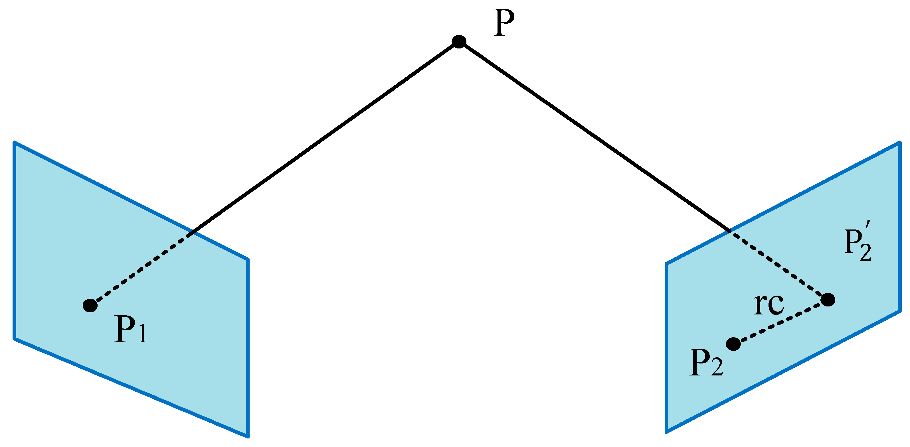
To achieve more accurate state estimation by fully utilizing both visual and IMU data, the IMU residual $r_I$ and the visual residual $r_v$ should be integrated into a unified error vector:

$$r=\left[\begin{array}{c}{r}_I\\ r_v\end{array}\right]$$

(13)

Its covariance matrix is given by

$$P=\left[\begin{array}{cc}{P}_I& P_{I,V}\\ P_{I,V}^T& P_V\end{array}\right]$$

(14)

where $P_{I,V}$ represents the covariance between the IMU prediction and the visual measurements.

3.2. Schur Complement

The Schur complement is an important concept in linear algebra, and is widely used in matrix decomposition, optimization problems, numerical computation, and fields such as SLAM. Its core idea is to eliminate certain variables through block matrix operations, thereby reducing computational complexity and improving the efficiency of numerical solutions. Compared to Cholesky decomposition, which typically operates on the entire system and often struggles to efficiently eliminate local variables while preserving sparsity, the Schur complement enables the selective marginalization of specific variables (such as feature points or past states). This significantly reduces computational overhead and better preserves the sparse structure of the system. As a result, it is particularly well-suited for scenarios involving frequent marginalization and sliding window optimization, as commonly encountered in visual SLAM.

In the optimization process of visual–inertial SLAM, it is necessary to estimate both the camera pose and the positions of three-dimensional feature points simultaneously. The dimension of the joint state variables is extremely high, and a direct solution typically involves enormous computational effort. To avoid directly handling all state variables, the Schur complement is introduced to marginalize the portion of the joint residual model related to the feature points, yielding a residual term that is only dependent on the camera pose. In other words, the Schur complement is used to eliminate certain variables, thus simplifying the computation process. Therefore, we use the Schur complement to accelerate the computation. During this process, the weighted squared error is minimized, where

$$\delta X=\arg \underset{\delta X}{min}{\displaystyle \frac{1}{2}}\parallel r-H\delta X{\parallel }^2$$

(15)

The error state $\delta X$ is used to update the estimated state, where $r$ is the constant term of the overall error, and $H$ is the Jacobian matrix of the residual with respect to the state variables.

Assume that the optimization variables are also divided into two parts:

$$\delta X=\left[\begin{array}{c}\delta X_i\\ \delta X_v\end{array}\right]$$

(16)

The optimization problem can be expressed as

$$\left[\begin{array}{cc}{H}_{I,i}& H_{I,v}\\ H_{v,i}& H_{v,v}\end{array}\right]\left[\begin{array}{c}\delta X_i\\ \delta X_v\end{array}\right]=\left[\begin{array}{c}{r}_I\\ r_v\end{array}\right]$$

(17)

The system of equations is computationally expensive to solve directly; therefore, the Schur complement can be used to eliminate the visual states $\delta X_v$ and solve for $\delta X_i$:

Solve for $\delta X_v$ using the second equation expanded from the above formula:

$$H_{v,v}\delta X_v=r_v-H_{v,i}\delta X_i$$

(18)

If $H_{v,v}$ is invertible, then the following can be obtained:

$$\delta X_v=H_{v,v}^{-1}\left(r_v-H_{v,i}\delta X_i\right)$$

(19)

Substitute this into the first equation:

$$H_{I,i}\delta X_i+H_{I,v}\delta X_v=r_I$$

(20)

The following can be obtained:

$$H_{I,i}\delta X_i+H_{I,v}{H}_{v,v}^{-1}\left(r_v-H_{v,i}\delta X_i\right)=r_I$$

(21)

Upon rearrangement, the following can be obtained:

$$\left(H_{I,i}-H_{I,v}{H}_{v,v}^{-1}\right)\delta X_i=r_I-H_{I,v}{H}_{v,v}^{-1}{r}_v$$

(22)

where

$${\dot{H}}_I=H_{I,i}-H_{I,v}{H}_{v,v}^{-1}$$

(23)

$${\dot{r}}_I=r_I-H_{I,v}{H}_{v,v}^{-1}{r}_v$$

(24)

This results in an equation that contains only the IMU state $\delta X_i$:

$${\dot{H}}_I\delta X_i={\dot{r}}_I$$

(25)

After solving for $\delta X_i$,we can substitute the result back to solve for $\delta X_v$:

$$\delta X_v=H_{v,v}^{-1}\left(r_v-H_{v,i}\delta X_i\right)$$

(26)

In this way, only a smaller linear system needs to be solved, thereby improving computational efficiency.

3.3. Iterative Update of IEKF

The IEKF improves the accuracy and stability of the fusion between vision and IMU by leveraging the high-frequency predictions from the IMU and the global corrections from vision, along with iterative optimization for measurement updates. This makes it suitable for tasks such as SLAM, robot localization, and autonomous driving.

In EKF, the measurement update is performed only once, whereas IEKF iteratively optimizes the estimation through multiple iterations. The initial state estimate is denoted as $X_k^{-}$, the initial covariance as $P_k^{-}$, and the iteration count is set as $i$.

$$X_k^{-}=f\left(X_{k-1},u_k\right)$$

(27)

$$P_k^{-}=F_k{P}_{k-1}^{+}{F}_k^T+Q_k$$

(28)

Iterative computation is performed to calculate the measurement prediction.

$${\widehat{y}}_k^{\left(i\right)}=h\left({\widehat{x}}_k^{\left(i\right)}\right)$$

(29)

The measurement Jacobian matrix is as follows:

$$H_k^{\left(i\right)}={\left.{\displaystyle \frac{\partial h}{\partial x}}\right|}_{x={\widehat{x}}_k^{\left(i\right)}}$$

(30)

Residual (innovation term):

$$r_k^{\left(i\right)}=y_k-{\widehat{y}}_k^{\left(i\right)}+H_k^{\left(i\right)}\left({\widehat{x}}_k^{\left(i\right)}-{\widehat{x}}_k^{-}\right).$$

(31)

Calculate the Kalman Gain:

$$K_k^{\left(i\right)}=P_k^{-}{H}_k^{\left(i\right)T}{\left(H_k^{\left(i\right)}{P}_k^{-}{H}_k^{\left(i\right)T}+R_k\right)}^{-1}.$$

(32)

Update the state estimate:

$${\widehat{x}}_k^{\left(i+1\right)}={\widehat{x}}_k^{-}+K_k^{\left(i\right)}{r}_k^{\left(i\right)}.$$

(33)

After the Schur complement-based acceleration step, the corresponding solution $\delta X$ is obtained. If the value of $\delta X$ is smaller than the predefined threshold, the state update is considered to have converged, and the iteration stops. Otherwise, set $i=i+1$ and continue the iteration.

When the iteration converges, the final updates for the state and covariance matrices are performed as follows:

$$X_k^{+}=X_k^{-}+K_k\left(z_k-h\left(X_k^{-}\right)\right)$$

(34)

$$P_k^{+}=\left(I-K_k{H}_k\right)P_k^{-}$$

(35)

The pseudocode of the algorithm proposed in this paper is shown in Algorithm 1. The algorithm proposed in this paper takes IMU prediction as the guide, integrates visual and inertial information by constructing joint residual and Jacobian matrix, and uses the Schur complement to marginalize some visual variables to reduce the optimization dimension. It then performs an iterative state update to improve the ability to handle nonlinear errors, and finally updates the state and covariance to achieve accurate and efficient visual–inertial state estimation.

Algorithm 1 Pseudocode of iterative Extended Kalman Filter based on Schur complement.

1. Inputs: a_k, ω_k, z_k^I, x0, P0 2. Initialize: x ← x0, P ← P0 3. For each time step k: 4.  Propagate x with IMU pre-integration 5.  Compute F, Q 6.  P ← F P FT + Q 7.  For each sliding window: 8.   Linearize residual: r = z − h(x) 9.   Construct Jacobian H, information matrix Λ 10.  Compute normal equations: 11.    HT Λ H δx = HT Λ r 12.   Apply Schur complement to marginalize landmarks: 13.    H_schur δx_s = b_schur 14.   For i = 1 to MaxIter: 15.    Solve for δx_s 16.    x ← x ⊕ δx_s 17.    If ||δx_s|| < ε: break 18.  Update covariance P via IEKF posterior 19. Output: Optimized state x and covariance P

It is worth emphasizing that the IEKF is a local optimization method whose convergence is not inherently guaranteed. The IEKF achieves local convergence when the initial estimate is sufficiently close to the true state, the measurement Jacobian is well-conditioned, and the noise covariances are properly bounded [28]. Under these conditions, the iteration converges quadratically to the local minimum of the nonlinear least squares problem. In practice, we apply a convergence threshold ϵ and terminate the iteration when $\delta X$ < ϵ, ensuring both computational efficiency and robustness.

4. Experimental Results and Analysis

To evaluate the effectiveness of the proposed algorithm, a series of experiments were conducted, including image-matching tests, trajectory estimation on public datasets, and validation on self-collected sequences. The image-matching experiment evaluated the feature extraction and matching performance after the introduction of MLP and Transformer architectures. The visual–inertial odometry trajectory experiment analyzed the stability and robustness of the algorithm in different dynamic environments. The public dataset experiment compared and analyzed the estimation accuracy of the algorithm in different dynamic environments and compared it with existing methods. The self-collected dataset experiment verified the generalization ability and robustness of the algorithm in real scenes. Collectively, these experiments demonstrate the proposed algorithm’s advantages in terms of accuracy, real-time performance, and adaptability to dynamic environments.

Simulation platform: The simulation platform utilizes a computer equipped with an Intel i7-13700H processor, 16 GB RAM, and an RTX3050 graphics card with 4 GB of VRAM. The software environment consists of Ubuntu 22, Docker, C++17, Python 3.8.5, and ROS2 Humble.

4.1. Matching Experiment

Image-matching experiments are carried out under different lighting conditions and viewing angle changes to evaluate the matching accuracy of the enhanced ORB feature points under these environmental changes.

Experimental setup: The ORB feature extraction module was configured to run on the GPU for acceleration. Some key parameters are as follows: the number of feature points extracted per image was set to 3000; the scale factor of the image pyramid was set to 1.2; and the number of pyramid levels was set to 8.

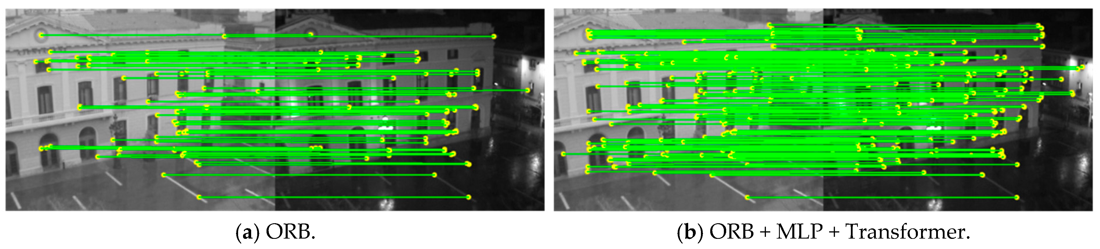
The experimental results presented in Figure 3 and Figure 4 demonstrate that, under varying lighting conditions and viewpoint changes, the ORB feature points enhanced by MLP and Transformer show significant improvements. The enhanced feature points can maintain high matching accuracy under uneven illumination or large perspective changes, improving the robustness and adaptability of the feature points. It is verified that the enhanced algorithm can significantly improve the stability and accuracy of feature matching in complex environments, providing reliable feature support for subsequent visual inertial pose estimation.

In order to test the operating efficiency, a video sequence from the KITTI dataset was tested, and the relevant results are presented in Table 1. The experimental results indicate that, under identical test conditions, the enhanced algorithm achieves a notable improvement in both the number of raw and correct matches, while incurring only a minimal increase in runtime. Specifically, when the number of extracted feature points was increased by 1000 compared to the conventional setting (typically 2000 points), the processing time increased by only 17 ms. This demonstrates the strong parallel computing capability and execution efficiency of the experimental platform, further validating the real-time performance and robustness of the proposed approach.

Table 1. Average per-frame results of different methods on the KITTI dataset.

Method	ORB	OURS
inliers	515.37	730.77
raw matches	911.23	1044.44
extraction time (ms)	10.9	27.3

Table 1. Average per-frame results of different methods on the KITTI dataset.

Method	ORB	OURS
inliers	515.37	730.77
raw matches	911.23	1044.44
extraction time (ms)	10.9	27.3

4.2. Visual–Inertial Odometry Trajectory Experiment

Visual–inertial odometry (VIO) is a pose estimation technique that combines visual information from a camera with inertial data from an IMU (Inertial Measurement Unit) to determine the motion of a mobile device. It estimates the relative displacement and orientation changes by detecting and tracking feature points across consecutive frames while integrating inertial measurements to improve accuracy and robustness. To further evaluate the performance of the proposed algorithm, trajectory reconstruction experiments were conducted in dynamic environments. The results demonstrate the algorithm’s stability and robustness in complex and challenging scenarios.

Experimental setup: The experiments were conducted using a laptop equipped with an RTX 3050 GPU. The number of feature points extracted per image was set to 2000; the scale factor of the image pyramid was set to 1.2; the number of pyramid levels was set to 8; and the feature-matching quality threshold was set to 0.7.

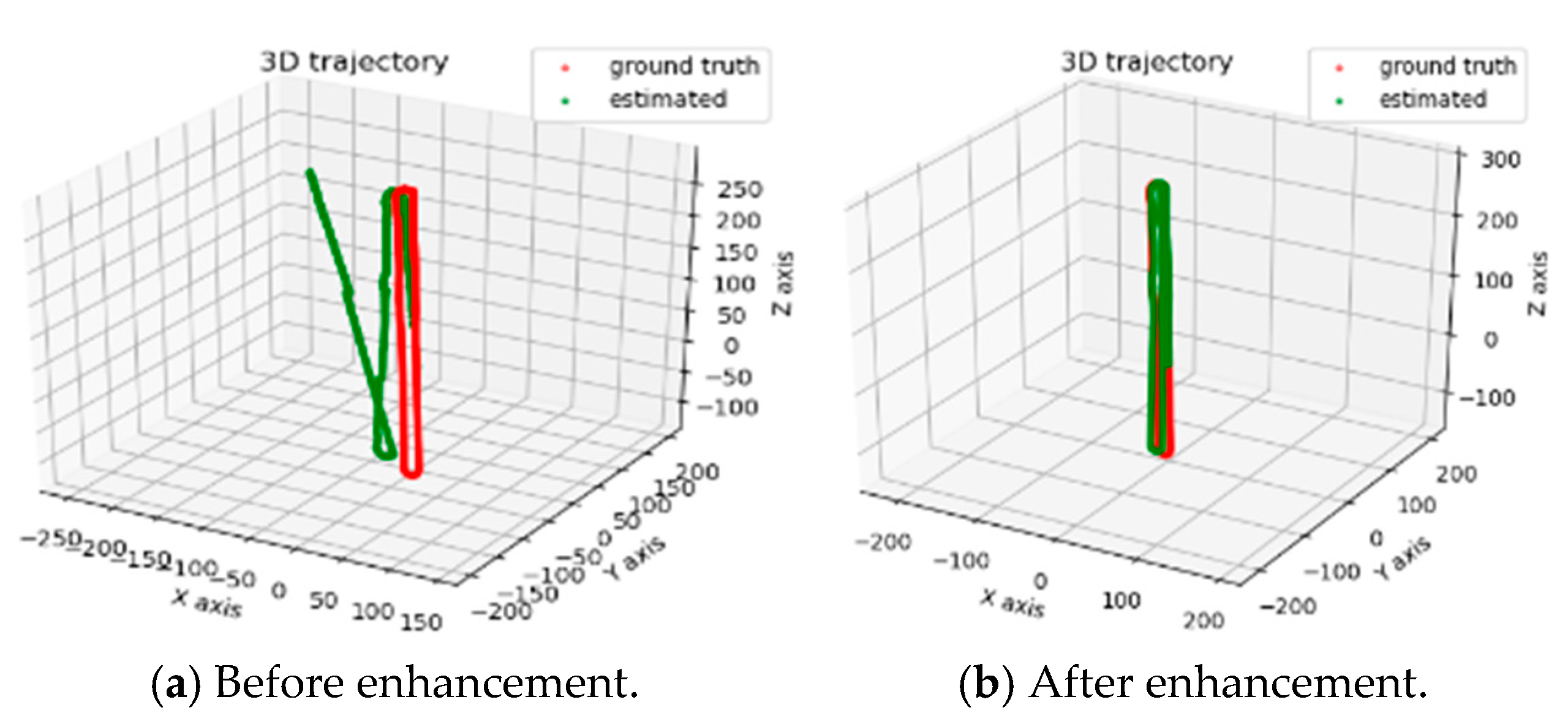
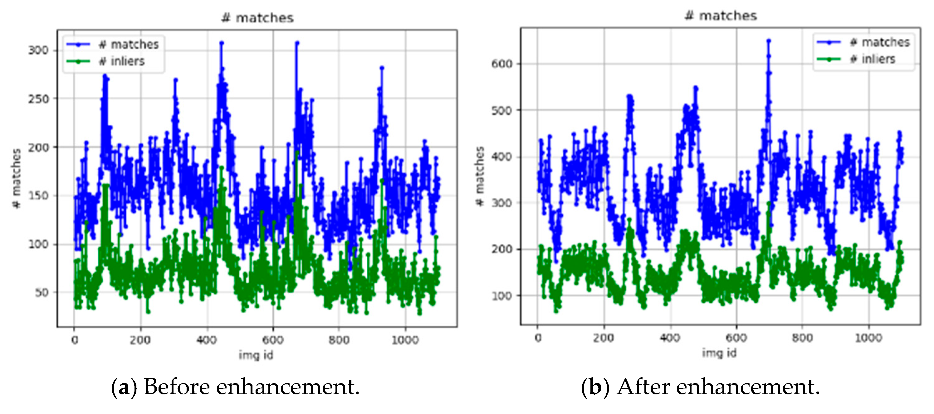
Figure 5a,b illustrate the trajectory results before and after applying the enhancement, respectively. Figure 6 compares the performance of the original and enhanced algorithms in terms of feature extraction, initial matching, and inlier matching. Figure 7 illustrates the errors of the original and enhanced trajectories along the x, y, and z axes relative to the ground-truth values.

The experimental results presented in Figure 5 demonstrate the performance differences before and after enhancement. In Figure 5a, the trajectory error remains small during the initial stage of the sequence but exhibits significant drift in the latter half. This drift becomes particularly severe in scenarios with large numbers of dynamic objects such as pedestrians and vehicles, leading to rapid error accumulation and poor robustness. In contrast, Figure 5b shows that the trajectory error remains within a relatively small range throughout the entire sequence, indicating a significant improvement in stability under dynamic environments. A comparison between Figure 6a,b clearly shows that the enhanced algorithm achieves a substantial increase in both the number of initial matches and inlier matches. Furthermore, Figure 7a,b reveal that, while the original algorithm suffers from continuously increasing error along the x-axis in the later stages, the enhanced algorithm maintains more stable error control in the x-direction, which is more susceptible to interference from dynamic objects. These results verify the robustness and improved accuracy of the enhanced method in complex, dynamic scenes.

4.3. Experiments on Public Datasets

In the pose estimation experiments using public datasets, the publicly available KITTI dataset was used for testing to evaluate the algorithm’s performance in real-world scenarios. EKF and IEKF were respectively employed for trajectory estimation experiments, and the differences in pose estimation accuracy between the two methods were compared. The corresponding root mean square error (RMSE) was calculated to quantitatively analyze the error performance of the algorithms. The formula for RMSE is as follows:

$$RMSE\left(x_n\right)=\sqrt{{\displaystyle \frac{{\left(x_n-x_{ngt}\right)}^2+{\left(y_n-y_{ngt}\right)}^2}{2}}}$$

(36)

$$RMSE\left(Average\right)={\displaystyle \frac{1}{N}}\sum _{i=1}^{N}RMSE\left(x_i\right)$$

(37)

In the above equation, represents the x-axis coordinate, represents the y-axis coordinate, the subscript denotes the actual coordinates of the algorithm at time step n, and ngt represents the ground truth coordinates at time step n. N denotes the number of data points in the dataset.

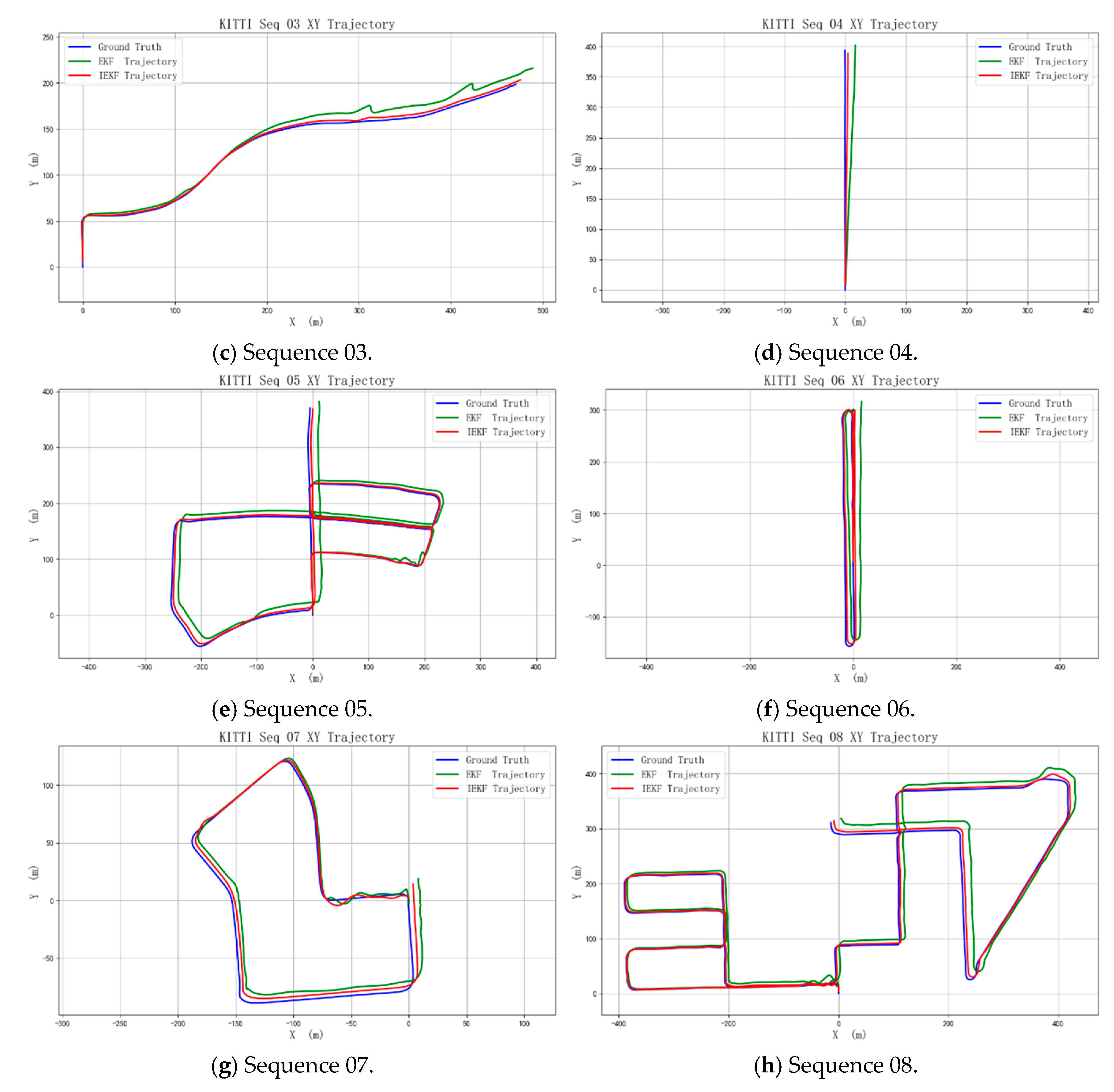
The EKF and the improved IEKF algorithms were applied to process sequences 00, 02, 03, 04, 05, 06, 07, and 08 of the KITTI dataset, as shown in Figure 8. The results indicate that the EKF estimated trajectory exhibits significant deviation from the true trajectory, while the trajectory estimated by the IEKF algorithm demonstrates much smaller errors, reflecting the higher accuracy of the IEKF.

The results of the attitude accuracy indicator, root mean square error (RMSE), can be found in

Table 2. RMSE statistics (m) of EKF and IEKF on the KITTI dataset.

Seq	00	02	03	04	05	06	07	08
EKF	0.258	0.154	0.259	0.212	0.350	0.320	0.528	0.497
IEKF	0.156	0.103	0.167	0.148	0.130	0.105	0.186	0.137

. The proposed method in this paper shows better estimation accuracy than the traditional EKF algorithm on eight test sequences randomly selected from the KITTI dataset. Specifically, the RMSE of IEKF in each sequence is lower than that of EKF, indicating that it is more robust and accurate in dealing with nonlinear systems and fusing visual and inertial information. This result fully verifies the effectiveness of IEKF in attitude estimation, and proves that it can improve the overall state estimation performance of the system compared with the traditional EKF in practical applications.

To evaluate the real-time performance of the algorithm, multiple test runs are conducted to reduce random errors in runtime measurements. Statistical comparisons of different algorithms are performed on sequences 00 to 10 of the KITTI dataset. The average runtime of the EKF is 2.62 s, while the IEKF takes an average of 3.93 s. In contrast, the BA-based optimization with a sliding window shows a significantly higher average runtime of 23.59 s. The test results are shown in Figure 9.

The results show that EKF achieves the fastest computation due to its low computational complexity but suffers from limited accuracy. The sliding window BA optimization offers higher accuracy but comes with a significantly increased computational load and the longest runtime. In contrast, IEKF strikes a balance by improving accuracy through iterative optimization while maintaining reasonable computational efficiency, demonstrating its advantage in both performance and practicality.

4.4. Validation Through Real-World Vehicle Tests

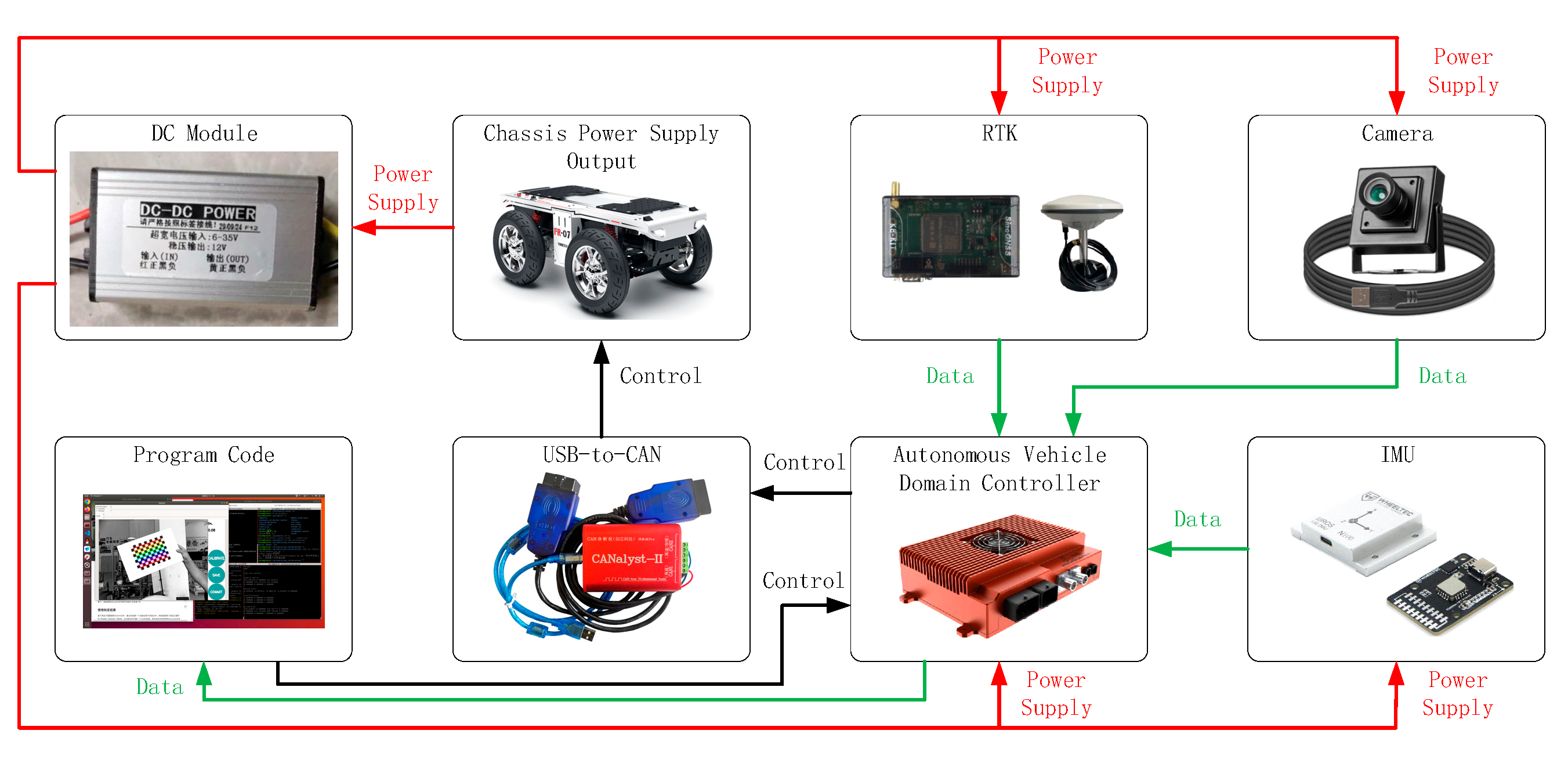
To further validate the practical applicability of the algorithm, a visual–inertial SLAM experimental platform was built based on an intelligent driving suite. The topological diagram of the experimental platform is shown in Figure 10. In the power supply topology, the output of the chassis with a battery is 48 V. To meet the power supply requirements of various sensors, a DC-DC module is used for voltage conversion, which steps down the 48 V to a stable 12 V output. The converted 12 V power is used to supply sensors such as the domain controller, camera, IMU, and RTK, as indicated by the red connecting lines in the diagram. In the data topology, the camera, IMU, and RTK sensors send their data back to the vehicle’s domain controller, as shown by the green connecting lines. The domain controller processes the data through software and outputs control signals. These control signals are transmitted via the domain controller to the CAN card, thereby controlling the vehicle, as indicated by the black connecting lines.

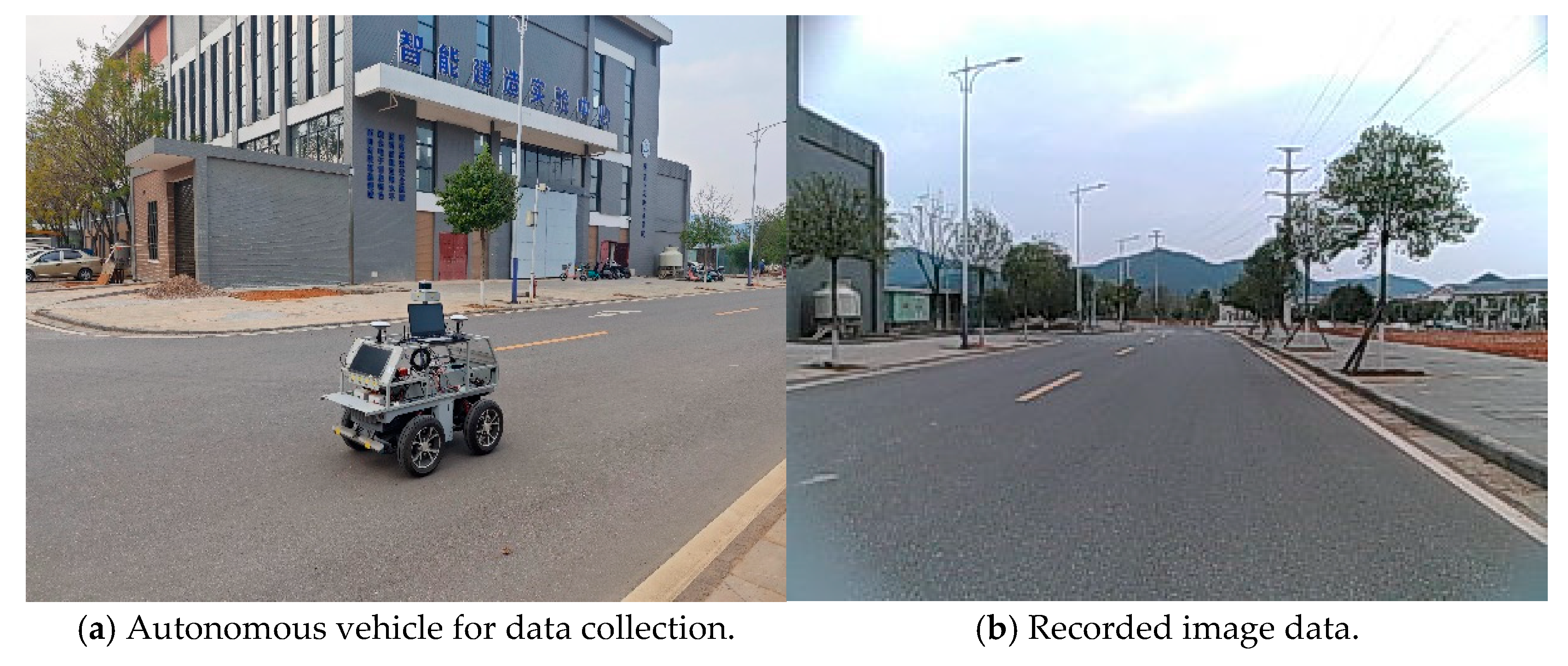
After the experimental platform was established, data collection was conducted on the regular driving routes within the campus to evaluate the performance of the EKF and IEKF algorithms in pose trajectory estimation. The overall route map is shown in Figure 11. Figure 12a shows a photo taken during the data collection process, which includes the autonomous vehicle used for data acquisition and the actual environment during the data collection. Figure 12b displays the image data from the self-collected dataset.

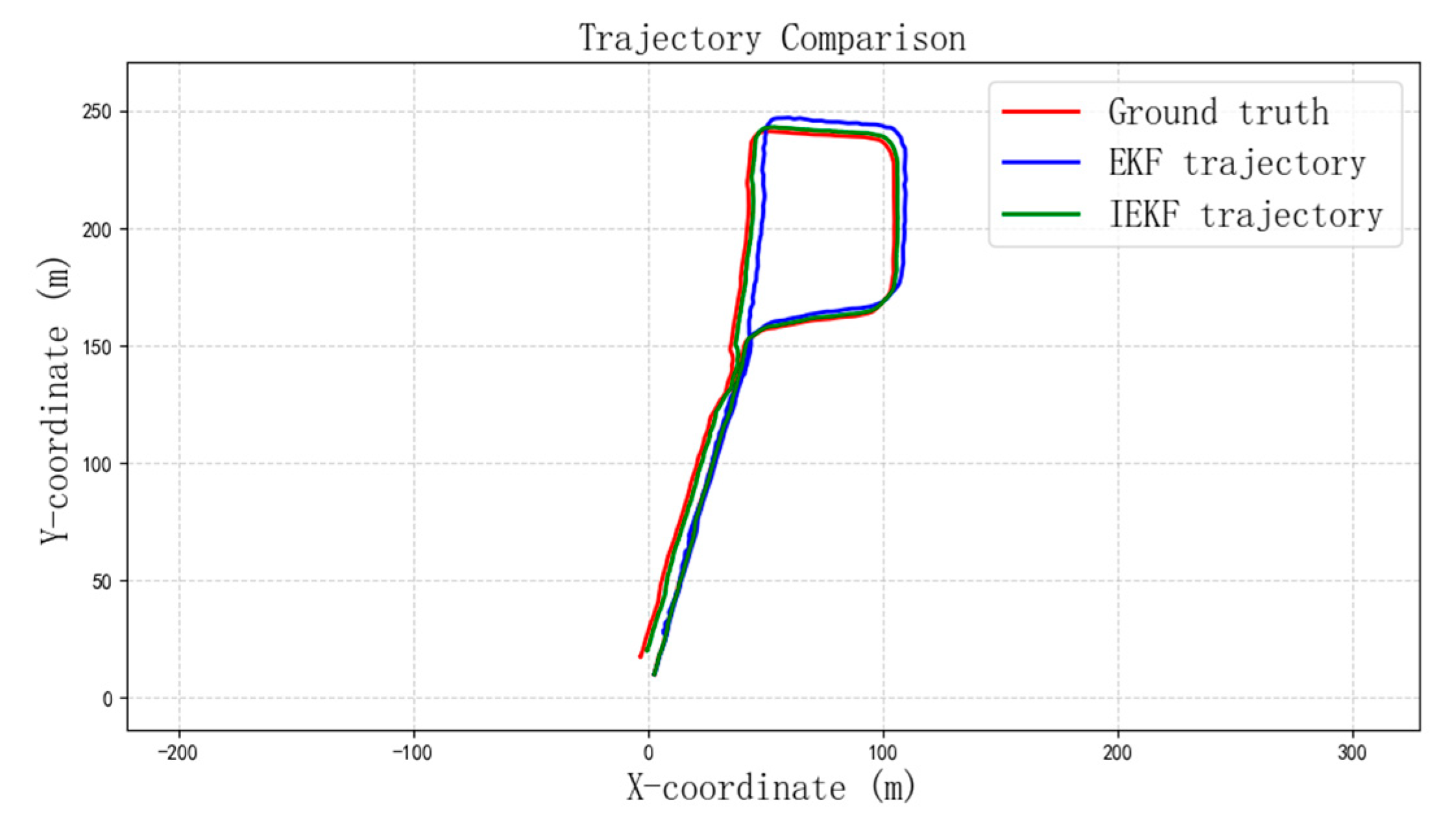
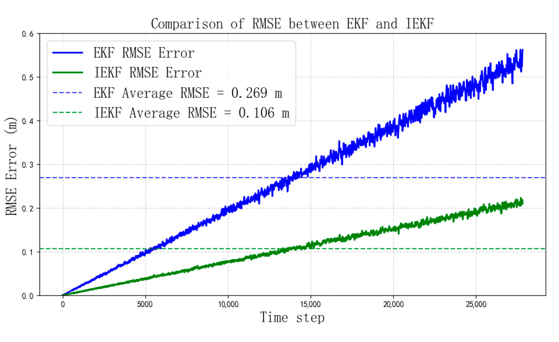
As shown in Figure 13, in the trajectory estimation, the EKF trajectory clearly deviates more from the real data compared to the IEKF trajectory. This indicates that the IEKF algorithm has higher accuracy than the EKF algorithm. According to Figure 14, the RMSE of EKF is 0.268 m, while the RMSE of IEKF is 0.106 m. The error of IEKF is 60.45% lower than that of EKF, representing a significant error reduction. The overall performance of the self-collected dataset is similar to that of the public dataset tests, aligning with the simulation’s expectations. This suggests that the proposed improved algorithm maintains a high level of accuracy and low error, even with a slight sacrifice in computational speed.

5. Conclusions and Future Work

In this paper, a pose estimation model based on the Iterated Extended Kalman Filter (IEKF) is developed to enhance the accuracy and robustness of visual–inertial odometry (VIO). The system integrates visual reprojection error and inertial measurement error into a unified framework and models the state variables accordingly. To improve computational efficiency, Schur complement optimization is introduced to marginalize high-dimensional variables, significantly reducing the computational overhead in large-scale SLAM problems. The main scientific contributions of this work include the following:

• The integration of Schur complement acceleration into the IEKF update process for efficient marginalization;
• The development of a visual–inertial odometry system with feature enhancement based on MLP and Transformer architectures. An MLP is incorporated into the traditional VIO framework to perform self-enhancement of feature descriptors, improving the matching robustness of individual keypoints under viewpoint and illumination changes;
• The demonstration of improved robustness and adaptability through extensive experiments across multiple datasets.

The experimental results demonstrate that the proposed algorithm outperforms traditional EKF-based methods in both accuracy and stability, especially in dynamic environments with moving objects. For instance, the algorithm maintains lower trajectory error (measured by RMSE) and higher matching accuracy while maintaining near real-time performance. Compared to conventional BA-based optimization, it achieves a good balance between efficiency and precision, with an average runtime significantly lower than that of full BA methods. These results validate the algorithm’s ability to provide reliable pose estimation under challenging conditions.

In future research, more advanced nonlinear optimization methods, such as Extended Kalman Filtering based on adaptive iteration strategies or learning-based filters, will be explored to further improve state estimation accuracy. Additionally, in large-scale SLAM tasks, the combination of sparse optimization or distributed computing frameworks could be employed to reduce computational complexity and enhance system scalability.