Article

Hard Preloaded Duplex Ball Bearing Dynamic Model for Space Applications

by
Pablo Riera
1,2,*,
Luis Maria Macareno
1,
Igor Fernandez de Bustos
1 and
Josu Aguirrebeitia
1
1
Department of Mechanical Engineering, University of the Basque Country, Plaza Ingeniero Torres Quevedo, 1, 48013 Bilbao, Spain
2
Department of Electromechanical Systems, Sener Aerospace, Avda Zugazarte 56, 48930 Las Arenas, Spain
*
Author to whom correspondence should be addressed.
Machines 2025, 13(7), 581; https://doi.org/10.3390/machines13070581
Submission received: 5 June 2025 / Revised: 30 June 2025 / Accepted: 2 July 2025 / Published: 4 July 2025
(This article belongs to the Section Machine Design and Theory)

Abstract

Duplex ball bearings are common components in space satellite mechanisms, and their behaviour impacts the overall performance and reliability of these systems. During rocket launches, these bearings suffer high vibrational loads, making their dynamic response essential for their survival. To predict the dynamic behaviour under vibration, simulations and experimental tests are performed. However, published models for space applications fail to capture the variations observed in test responses. This study presents a multi-degree-of-freedom nonlinear multibody model of a hard-preloaded duplex space ball bearing, particularized for this work to the case in which the outer ring is attached to a shaker and the inner ring to a test dummy mass. The model incorporates the Hunt and Crossley contact damping formulation and employs quaternions to accurately represent rotational dynamics. The simulated model response is validated against previously published axial test data, and its response under step, sine, and random excitations is analysed both in the case of radial and axial excitation. The results reveal key insights into frequency evolution, stress distribution, gapping phenomena, and response amplification, providing a deeper understanding of the dynamic performance of space-grade ball bearings.

1. Introduction

Bearings are fundamental components in rotating systems, typically operating under vibrations induced by rotary motion. These vibrations originate from external loads and mechanical interactions among machine elements, such as gears and shafts, as well as internal interactions involving rolling elements, rings, cages, and also the lubricant within the bearing. However, bearings in space applications must face a different type of vibration inherent to any type of space mechanism. This occurs primarily during rocket launch when the satellites remain enclosed within the rocket, representing the most critical scenario for space bearings. Ensuring bearing survival during this phase is essential for proper satellite operation throughout its lifetime. To achieve this, simulations and tests are usually performed under the following loads: a static acceleration load equivalent to the rocket acceleration during launch, sine loads and random loads related to the rocket vibration, and a shock load equivalent to the satellite’s deployment.
Double-row preloaded ball bearings form the joints between different movable components in space mechanisms. These bearings are arranged in either back-to-back or face-to-face configurations and can have either hard or soft preload, as described in [1]. Among all satellite bearings, they withstand the highest loads and their preload must provide adequate stiffness for the survival of the bearing during rocket launch, thereby enabling proper satellite operation during its life. The integrity of these bearings is assessed verifying the contact stresses and gappings along the vibration response. Moreover, the preload not only affects the vibrational response but also the friction, which selecting a much higher preload than the minimum required one implies a higher friction that decreases the motorization margin of satellite’s electrical motors. Therefore, accurate modelling of all these aspects is a key factor to assess the survival and operability of the bearings.
Different models have been developed to estimate the static load distribution and stresses in ball bearings. Sjovall [2] used finite element method (FEM) and a semi-analytical model to determine the radial load distribution within bearings. This model was later employed by Hernot et al. [3] to compute the bearing stiffness matrix and by Liu et al. [4] to asses load distribution and stiffness variations, incorporating ball preload and contact angle variations. Houpert [5,6] proposed point contact curve fitting approach for ball-raceway contacts, obtaining close results when comparing them with Hertz’s approach [7]. Regarding the explicit dynamic modelling, the use of finite element analysis (FEA) for point contact modelization is not feasible due to the required computational cost. Consequently, this work uses the analytical model developed by Hertz [7] for ball-raceway contact, along with the single-row ball bearing model developed by Harris and Kotzalas in [8,9] to develop the dynamic model. In this approach the dynamic forces are determined with the static model incorporating the contact damping effects.
In the field of bearing rotary dynamics, the current reference software is advanced dynamics of rolling elements (ADORE), developed by Gupta [10]. This multibody simulation tool models the contact between rolling elements, rings and cage providing key insights such as cage forces, accelerations and friction. Stacke et al. [11] developed bearing simulation tool (BEAST), a rolling bearing dynamic simulation tool which, in addition, includes other mechanical element forces for dynamic simulations. Xi et al. [12] proposed a multibody model for ball bearings to analyse the ball-raceway contact path under different conditions, concluding that the axial force plays a decisive role in the contact path distribution. Bizarre et al. [13] developed a bearing model simulating the elastohydrodynamic lubrication (EHL) contact evaluating the stiffness and damping characteristics of angular contact bearings under different conditions. Petersen et al. [14] proposed a double-row ball bearing model under radial loads to investigate the dynamics of the system under different raceway defects, demonstrating strong correlation with the performed experimental tests. Luo et al. [15] conducted dynamic simulations using FEA to analyse an angular contact ball bearing, incorporating the cage and balls at varying velocities to assess axial and radial stiffness. The simulations and the theoretical models showed agreement with the experimental data.
Rotor systems supported by a pair of bearings share structural design similarities with the hard-preloaded duplex bearings used in space applications, as both systems support a mass with two (bearing) rows. These rotor system models often incorporate bearing defects, rotor unbalance, preload variations and other excitations, with the damping defined either at a ball-raceway contact level, or through a global damping matrix for the entire bearing. Fang et al. [16] analysed the influence of the different bearing stiffness matrix elements on rotor dynamics, clarifying the effects of the off-diagonal elements comparing O (back-to-back) and X (face-to-face) configurations. Liu and Shao [17] developed a twelve degree of freedom rotor dynamic model considering housing stiffness, frictional moments and localized defects with particular focus on how housings properties affected the dynamics of the system across three different models. Cheng et al. [18] investigated the dynamics of the rotor considering radial clearance, rotor-stator rubbing, rotor eccentricity, raceway defects and waviness of the bearings. The study concluded that a higher preload improves the load distribution, the rubbing leads to a sharpening in the displacement signal, and waviness influences the system only at a specific velocity. Sinou [19] introduced a flexible shaft modeled by thirteen Timoshenko beam elements supported by two ball bearings, with an unbalanced disc attached to a flexible coupling. The study demonstrated the complexity of the nonlinear response for small changes in model parameters such as the radial clearance of the bearings. Young et al. [20] analysed the rotor stability under random axial forces employing FEA to discretize the equations and the Itô method [21,22] to obtain the responses, concluding that reducing the bearing axial forces increased system instability. Gao et al. [23] modeled a dual rotor system under barrel-roll flight loads, incorporating a defect in the outer raceway, proving the effects of the manoeuvre load, the defect and the rotating speed on the dynamic response.
Reaction wheel models also share similarities with the testing of space duplex bearings, as they support a high mass using two bearings and analyse system vibrational characteristics. Alkomy and Shan [24] developed a reaction wheel micro-vibration model, simulating imbalance and bearing waviness, with simulations accurately predicting system forces and moments in agreement with experimental results. Addari et al. [25] modeled a satellite cantilever reaction wheel which was validated with experimental results. The study highlighted the influence of the gyroscopic moment in the response of the system and proposed a methodology for the measurement of dynamic mass.
Rotor systems used for aeroengines response simulations also resemble the structural models of duplex bearings as they distribute different masses along the rotor supported by bearings. Chen [26] developed a coupled rotor-ball bearing-stator dynamic model to analyse aeroengine vibrations, incorporating contact nonlinearities. The model effectively simulated rubbing faults, which were validated through experimental tests. Hou et al. [27] investigated a dual rotor aeroengine system supported by five bearings with variable speed ratios, determining the bending-torsional coupling which affected the response. Lu et al. [28] proposed another dual-rotor system of an aeroengine with four bearings, considering faults in one of the masses and reducing the model order to obtain dynamic responses. The results provided accurate solutions compared to those of the complete model, enabling the development of an efficient computational tool for designing large rotor systems with significant masses.
The models described above assess the dynamics of the bearings related to their own rotation. However, a significant part of the vibratory behaviour of space bearings is driven by large inertial excitations during rocket launch, while they are not rotating. These excitations can be classified into an equivalent set of loads for their analysis and testing [29]: static acceleration load, sine load, random load and shock load. The common approach in the industry to analyse the bearing vibrations is to assume a linear stiffness for the bearing within the FEM and compute structural responses to the excitations by modal superposition. An alternative simplified method is using the Miles’ equation [30], which determines the response grms of the system under random vibrations. However, neither approaches can capture the system’s nonlinear effects to estimate the maximum load appearing in the response, therefore, the simplification of 3σstd approach [31] is used to determine random loads. While FEM and Miles’ method provide a fast estimation about resonances and accelerations, they cannot capture the changes on bearings damping and natural frequencies under varying load levels which have been appreciated in tests.
Experimental studies have also been conducted to assess the vibrational behaviour of ball bearings and validate theoretical models. In this context, Söchting et al. [32] performed harmonic axial vibration tests to measure the gapping between the rings of a ball bearing by means of two laser triangulation transducers. Additionally, friction measurements were carried out to evaluate the impact of vibrations on friction torque. The gapping results were compared to a linear axial model that integrated the stiffness obtained with Code for Analysis of Bearings in Rocket Engines Turbopumps (CABARET) [33], showing similar results for low load levels. However, for higher load levels, the predicted gappings were higher than the gappings obtained through the experiments. Munro et al. [34] performed a series of axial vibration tests to different configurations of back-to-back duplex space ball bearings. The bearings were tested in different setups: soft preloaded without snubber, soft preloaded with various snubbers and hard preloaded. The results indicated that increasing load levels led to corresponding changes in natural frequencies and response amplitudes.
Continuing with the study, Hinque and Seiler [35] developed perhaps the most complete work about axial vibrations of space bearings. He concluded that, for hard preloaded systems the gapping effect was almost linear, and that for soft preloaded systems it was necessary to simulate spring and snubber interactions to assess the nature of that gapping effect. Another key finding was that applying the rule of 3σstd to assess the maximum load in a random vibration may not be a reliable approach, as some instantaneous loads observed in tests significantly exceeded the limits stated by the rule. To further investigate these effects, Hinque developed a single degree-of-freedom (DOF) dynamic axial model of the bearing, using load level test results to correlate model parameters. While the model obtained good correlation for resonant frequencies at low load levels, it exhibited limited sensitivity to frequency variations, and the damping was represented with a global damping matrix rather than being modeled at the ball-raceway contact, where most of the damping actually occurs. Additionally, the model only accounted for the axial DOF, overlooking the radial behaviour, which is a critical factor in the overall performance of space bearings.
In this work, unlike previous models used for space applications, which rely on simplified representations such as linear stiffness assumptions or single-DOF dynamics, the proposed approach incorporates multiple-DOF, enabling the simulation of axial, radial and tilting combined responses, as well as non-centred masses and combined excitations. This multidirectional capability is essential to reproduce the complex dynamic behaviour experienced during satellite launches. The model includes contact-level damping at the ball–raceway interface using the Hunt and Crossley formulation, allowing a more accurate representation of energy dissipation compared to models that apply a global damping coefficient. Additionally, the use of quaternions to represent rigid body rotations eliminates the need for trigonometric functions, improving numerical stability and computational efficiency. These features collectively enhance the model’s ability to capture key nonlinear phenomena observed in experimental tests, such as shifts in natural frequencies, changes in transmissibility, stress and gapping effects under vibration.
In contrast to linear models, which provide constant natural frequencies and transmissibility values regardless of the load level or excitation type, the proposed model captures variations in both quantities as a function of the applied load. This difference arises because linear models rely on simplified amplification formulas directly related with a global damping, whereas the proposed model is based on an explicit formulation with damping directly applied at the ball–raceway contact. This representation allows to reproduce the nonlinear behaviour observed in tests in the simulations, capturing the cross-coupling effects. Moreover, compared to explicit models that incorporate damping as a general term based on the relative velocity between rings, the proposed approach integrates damping at the actual physical source of energy dissipation. By computing the local penetration velocities at the ball–raceway contacts, the model provides a more accurate and detailed representation of damping behaviour. The difference with general damping models increases when rotational dynamics are considered, where each ball dissipates a different amount of energy, an effect reproduced by the proposed model.
As a benchmark, this study takes the hard preloaded duplex bearing described in [35] which was tested in [34]. First, the static model of a duplex bearing is introduced revealing the geometrical nonlinearities of the system. Next, the ball-raceway contact damping model is presented, followed by the quaternion-based formulation used to describe the dummy mass dynamics. Afterwards, time dependent loads are applied to the model, revealing the changes on resonant frequencies and amplitudes showing strong correlation with the available axial vibration data [34]. The analysis is further extended to radial simulations, demonstrating that the model successfully captures the cross-coupling modes, whose influence is underlaying the results of those published axial tests. Finally, the conclusions of the developed model and performed simulations are presented.

2. Static Ball Bearing Model

This section presents the model for the static assessment of two-point contact ball bearings and its application in developing a double-row bearing model analyzing the stiffness under a specified preload.

2.1. Single-Row Ball Bearing

The duplex ball bearing model is based on the static single-row model developed by Harris and Kotzalas in [8,9]. In this model, the rings are considered rigid, as their stiffness is several orders of magnitude higher than the ball–raceway contact stiffness. Moreover, when the rings are mounted within housings and shafts using fits, their effective stiffness increases even further, reinforcing the validity of the rigid ring assumption. As a result, elastic deformation concentrates at the contact level, and ring flexibility can be neglected without compromising accuracy. This developed model by Harris and Kotzalas [8,9] is established upon one main fact: if the positions of the inner and outer ring are known, then, the ball-raceway static contact forces can be determined, and hence, the static force-deformation behaviour is characterized. In dynamic models, this static force-deformation behaviour is usually adopted also for time dependent simulations, yielding accurate results. The model consists of Z balls positioned at defined angles ψ. The adopted reference frame is defined such that the X-axis aligns with the bearing axis, the Y-axis is vertical, and the Z-axis is oriented according to the right-hand rule established by the previous axes. For specific displacements of the inner ring ζx, ζy, ζz and rotations ϕy, ϕz relative to the outer ring (in the free displaced position), the position of the center of curvature of the inner raceway is calculated for the location of each ball, written as:
s a x i a l = A · sin α o + ζ x + R i · ϕ y · s i n ψ R i · ϕ z · c o s ( ψ )   and
s r a d i a l = A · cos α o + ζ y · cos ψ + ζ z · s i n ( ψ ) .
Then, the distance between the centers of curvature of the inner and outer raceways is calculated along with the working contact angle α and ball penetration:
s = s a x i a l 2 + s r a d i a l 2 ,
α = arcsin s a x i a l s   and
δ b a l l = s A .
This last Equation (5) determines the total penetrations at the inner and outer contacts. A positive value indicates penetration, while a negative value denotes gapping.
With the working contact angle α, the curvatures ρ involved in inner and outer contacts are calculated. These curvatures are then used to compute the curvature sum Σρ and the curvature difference F(ρ) for inner and outer contacts, following the methodology described in [8]. Based on F(ρ), the dimensionless parameters a*, b*, δ* for inner and outer contacts are obtained by interpolating the values from a previously constructed lookup table as outlined in [8]. Using these values, the stiffness of outer and inner contacts is calculated through the equations:
δ i / o = δ i / o * · 3 · Q i / o 2 · ρ i / o · 1 v I 2 E I + 1 v I I 2 E I I 2 3 · ρ i / o 2 Q i / o = 2 5 2 3 · E · ρ i o 1 2 · δ i o * 3 2 δ i / o 3 2 Q i / o = k i / o · δ i / o 3 2   and
k i / o = 2 2 3 2 3 E Σ p i / o 1 2 δ i / o * 3 2 .
The center of the ball is placed between the centers of curvature of the two rings, with the loads Qi and Qo being equal. Therefore, the total stiffness kball, which accounts for outer and inner contacts, is determined using the equation:
k b a l l = 1 1 k i 2 3 + 1 k o 2 3 3 2   and
the load Q for each ball as a function of the total penetration δball is calculated with:
Q = Q i = Q o = k b a l l · δ b a l l 3 2 .
Finally, given the load Q in each ball j, the contact angle α, the ball angular position ψ and the pitch diameter dm, the forces and moments acting on the outer ring are calculated with:
F x = j = 1 z Q j · s i n ( α j ) ,
F y = j = 1 z Q j · cos α j · cos ψ j ,
F z = j = 1 z Q j · cos α j · s i n ( ψ j ) ,
T y = d m 2 · j = 1 z Q j · sin α j · s i n ( ψ j )   and
T z = d m 2 · j = 1 z Q j · sin α j · c o s ( ψ j ) ,
noting that the inner ring forces are opposite.
With this model, the rings are considered as rigid bodies, while all deformation occurs at the ball-raceway contact interface. Each ball is represented by a nonlinear traction spring that simulates Hertzian contact and gapping, with the ends of these springs connected to the centers of curvature of each raceway. These curvature centers are rigidly connected with their respective rings. When the relative position and rotations between the rings are known, the contact forces of the bearing can be calculated. This approach has been extensively used, as discussed in Section 1, and it has even been implemented in finite element models as described, among others, in [36].

2.2. Duplex Bearing

Figure 1 illustrates the preloaded configuration of the back-to-back duplex bearing system, including inner and outer spacers. The black geometry corresponds to the initial state, in which the hard preload has already been imposed. The red overlay represents a displacement applied to the inner ring simulating an applied load to this ring while the outer ring remains fixed.
To model this configuration, six nodes are defined in the system. Three nodes are attached to the fixed outer ring (with the o subindex): one is located at the center of the duplex (C subindex), and the other two are placed symmetrically at a distance of W/2 from the center, left and right nodes with L and R subindexes, as defined in the following equation in the center reference system of the bearing (SF):
x c o y c o z c o φ y c o φ z c o S F = 0 0 0 0 0 ,   x L o y L o z L o φ y L o φ z L o S F = W 2 0 0 0 0   a n d       x R o y R o z R o φ y R o φ z R o S F = W 2 0 0 0 0 .
The remaining three nodes are attached to the inner ring, with i subindex, one at the center and the other two at the center of each bearing row. In addition, three fixed reference frames are introduced: one located at the center of the duplex (denoted SF) and two at the center of each row (SL and SR), as shown in Figure 1.
Based on the inner ring center displacements xci, yci, zci and rotations φyci, φzci, the final position and rotations of the left (L) and right (R) inner ring node rows are obtained in the reference system located at the center of the duplex (SF) through the following relation:
x c i y c i z c i φ y c i φ z c i S F = x y z φ y φ z ,   x L i y L i z L i φ y L i φ z L i S F = x W 2 + ζ p r e l o a d y + W 2 + ζ p r e l o a d · sin φ z z W 2 + ζ p r e l o a d · sin φ y φ y φ z a n d   x R i y R i z R i φ y R i φ z R i S F = x + W 2 ζ p r e l o a d y + W 2 ζ p r e l o a d · sin φ z z W 2 ζ p r e l o a d · sin φ y φ y φ z .
Then, to compute the relative displacements and rotations of each row in each respective reference system the following equation is used:
ζ x L ζ y L ζ z L ϕ y L ϕ z L S L =   x L i y L i z L i φ y L i φ z L i S F x L o y L o z L o φ y L o φ z L o S F , ζ x R ζ y R ζ z R ϕ y R ϕ z R S R = x R i y R i z R i φ y R i φ z R i S F       x R o y R o z R o φ y R o φ z R o S F ,
which values are introduced to the single-row bearing model defined in Section 2.1 to obtain the reaction forces:
F x L F y L F z L T y L T z L = f o n e   r o w   m o d e l ζ x L , ζ y L , ζ z L , ϕ y L , ϕ z L S L ;   F x R F y R F z R T y R T z R = f o n e   r o w   m o d e l ζ x R , ζ y R , ζ z R , ϕ y R , ϕ z R S R .
With this model, as appreciated in previous Equation (18), the reactions on each row are calculated. After, those reactions, which are in each row respective reference systems are computed into the duplex center with the formula:
F x D F y D F z D T y D T z D S F = F x L F x R F y L + F y R F z L F z R T y L + T y R F z L · x L i x c i + F x L · z L i z c i + F z R · x R i x c i F x R · z R i z c i T z L T z R + F y L · x L i x c i F x L · y L i y c i + F y R · x R i x c i + F x R · y R i y c i ,
obtaining the forces acting the output ring of the duplex.
The preload is a key factor in the model, as it directly influences the stiffness, stresses and response of the system to dynamic excitations. To account for this effect, an initial positive displacement ζpreload is applied to the inner rings of each row within their respective reference systems, as noted in Equation (16). As the duplex configuration depicted in Figure 1 follows back-to-back arrangement, the preload involves an initial positive displacement for the inner ring left node and a negative displacement for the inner ring right node in the SF reference frame.
For the duplex bearing described later in Section 5, Figure 2 presents the stiffness for axial, radial and bending loads. These graphs highlight the nonlinear characteristics of the bearing, which significantly affect the dynamic response of the system. Two types of stiffnesses are defined in the graphs. The finite stiffness is determined as the derivative of the force with respect to the displacement, capturing local variations in stiffness. The linearized stiffness is calculated as the load divided by the corresponding displacement, which presents a smaller variation and is the conventional parameter used in finite element (FE) models to represent bearing behaviour.

3. Dynamic Ball Bearing Model

In this section, the static models in Section 2 are extended to obtain the corresponding dynamic models. For this purpose, velocities and damping effects are included in the arrangement. The single-row and duplex models are adapted for dynamic analysis substituting Equation (9) with Equation (23).
In the models used in [16,18,19,20,21,22,23,24,25,26,35] the damping is included as a damping matrix for the whole bearing, relating the velocities of the inner and outer ring center nodes. This damping matrix is then incorporated into the equations of motion. However, there is an alternative approach with more physical representation than treating the damping as a “black box”, which is considering the damping in the ball-raceway contact. This perspective is supported by the work of Dietl et al. [37], who performed different tests estimating the loss factor and concluded that damping was originated primarily from the ball-raceway contact interactions. Following this approach, studies such as [10,11,12,13,14,17] define the damping at each ball-raceway contact, offering a more accurate approach to model the damping behaviour in bearings. These contact damping models consider the effects of the lubricants and angular velocity of the bearing. Nevertheless, in this work the effect of EHL is not relevant, as the bearing is not rotating when it is suffering the vibration and the damping factor is adopted to account for all possible damping contributors.
Flores and Lankarani [38] and Corral et al. [39] reviewed the models for contact damping phenomena in multibody systems that may be closer for the conditions of simulation proposed in this work. Among those models, the one developed by Hunt and Crossley in [40] is selected. This Hertz-damp model is represented as:
Q c o n t a c t = k c o n t a c t · δ c o n t a c t 3 2 + 3 2 · γ · k c o n t a c t · δ c o n t a c t 3 2 · δ ˙ c o n t a c t   and
considers the effect of the contact load and the velocity of penetration for one contact. The first term of the equation is the Hertzian contact force, while the second term represents the damping force. The parameter γ is the damping parameter of the model and δ ˙ c o n t a c t is the penetration velocity.
However, in the bearing model each ball represents an inner and an outer contact. Therefore, the expression defined by Hunt-Crossley needs to be extended for the model of this work to consider both contacts in a single equation. The formulation for this adaption is presented in the following equations:
Q b a l l = Q H e r t z + Q D a m p i + Q D a m p o = k b a l l · δ b a l l 3 2 + 3 2 · γ · k i · δ i 3 2 · δ ˙ i + 3 2 · γ · k o · δ o 3 2 · δ ˙ o ,
Q H e r t z = k b a l l · δ b a l l 3 2 = k i · δ i 3 2 = k o · δ o 3 2   w i t h   δ ˙ b a l l = δ ˙ i + δ ˙ o ,   and
Q b a l l = k b a l l · δ b a l l 3 2 + 3 2 · γ · k b a l l · δ b a l l 3 2 · δ ˙ b a l l .
With this formulation, the single-row dynamic bearing model remains identical to the static model described in Section 2.1, except that Equation (9) is replaced by Equation (23). To complete the single-row dynamic model, the penetration velocity of the ball δ ˙ b a l l must be determined. Assuming the outer ring fixed, and given the inner ring velocities ζ x ˙ , ζ y ˙ , ζ z ˙ and angular velocities ϕ y   ˙ , ϕ z ˙ , the penetration velocity of the ball δ ˙ b a l l is determined using the equations:
s ˙ a x i a l = ζ ˙ x + R i · ϕ ˙ y · s i n ψ R i · ϕ ˙ z · c o s ( ψ ) ,
s ˙ r a d i a l = ζ ˙ y · cos ψ + ζ ˙ z · s i n ( ψ ) ,
s ˙ = s ˙ a x i a l 2 + s ˙ r a d i a l 2 ,
α s = a r c t a n 2 s ˙ r a d i a l , s ˙ a x i a l   and
δ ˙ b a l l = s ˙ · cos α s π 2 α .
It is important to note that the velocity of the inner ring center of curvature needs to be projected onto the line connecting inner and outer centers of curvature, which is done in Equation (28).
The dynamic model of the single-row bearing is then extended to the duplex bearing following the methodology described in Section 2.2. Given the defined duplex center inner ring velocities x ˙ , y ˙ , z ˙ and angular velocities ϕ y ˙ , ϕ z ˙ 
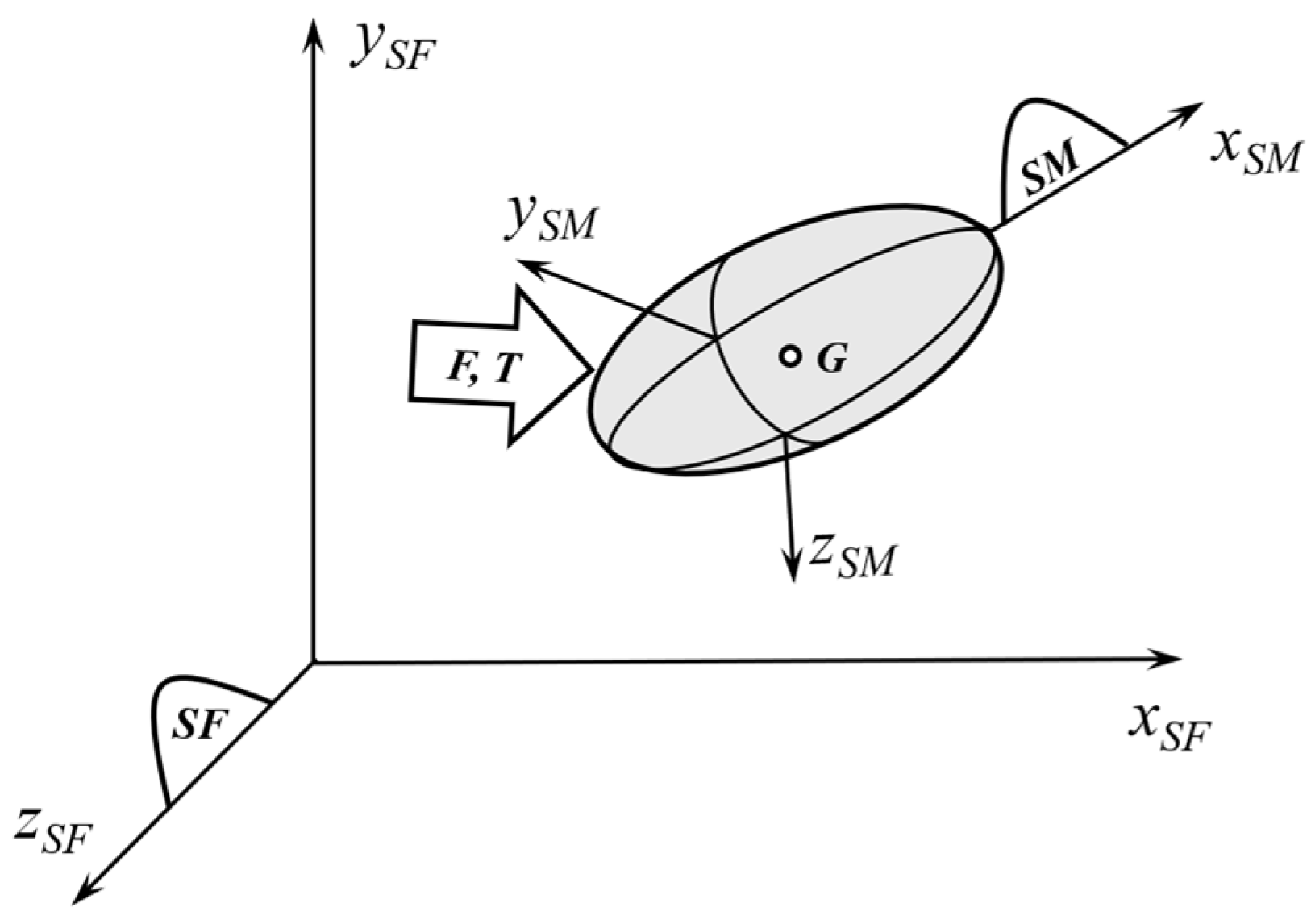
, the velocities of the left and right row inner nodes are determined. Then, these nodal velocities are translated to the reference frames of their corresponding row and they are introduced in the single-row model for force calculation. After, the forces of each row, including elastic and damping forces, are translated to the center of the duplex. Therefore, introducing to this complete model the inner ring displacements and velocities relative to the outer ring, the forces and moments at both rings are obtained. Moreover, these reactions already contain the static and damping forces of the bearing. Hence, the duplex model can be easily included in multibody dynamic simulations.

4. Duplex Test Vibration Model with Dummy Mass

Space mechanisms experience significant vibrations during satellite launches, primarily induced by the rocket boosters. For analysis and testing purposes, launch loads are usually divided into four different components [29]: static acceleration load, sine load, random load and shock loads. Dynamic testing of the satellites and their components is a crucial step in the development and qualification of space mechanisms. The rotating interfaces of these mechanisms, including actuators, robotic arms, gimbals and reaction wheels among others, are composed of duplex preloaded bearings that must withstand launch conditions to ensure the proper performance of the satellites. Consequently, the development of dynamic duplex models capable of simulating launch loads, which accurately reflect changes in natural frequencies and damping characteristics across varying load levels, represent an advancement for the space industry.
Testing of these mechanisms is performed by attaching a dummy mass, which possesses inertial properties equivalent to those of satellite components, to the output duplex bearing, as illustrated in Figure 3. Accelerometers are placed on both the shaker (control) and the dummy mass (response). The dynamic model comprises two distinct rigid bodies and three nodes, being the bearing the flexible element. The first rigid body represents the outer ring, which is fixed to the shaker and includes a single node at its center. The second body corresponds to the dummy mass, which is connected to the inner ring, and features one node at the center of the ring and another at the center of gravity G of the body. Consequently, the position and rotation of the dummy mass + inner ring over time can be simulated. Therefore, this section presents a dynamic explicit multibody model for the simulation of these hard preloaded duplex space bearings.

4.1. Explicit Iterative Process

In multibody dynamic analysis, a rotation system is required to accurately describe the orientation of the components such as the dummy mass dynamics. While different representations exist, quaternions offer a compact solution avoiding issues such as gimbal lock and numerical drift. Therefore, they are widely used in aerospace [41,42] and robotics [43] among others, for attitude control and smooth orientation tracking. In the field of dynamic analysis, quaternions are also explored together with the Hamiltonian formulation [44,45] to improve the multibody integration methods and are extended to rigid body dynamics in [46,47,48] analyzing the performance of the improved methods, as in the spinning of a top.
Considering the advantages provided by the quaternion q , this orientation system is selected to represent body rotations [49,50], as defined in the equation:
q = q 0 q 1 q 2 q 3 .
This choice is motivated by the simplicity of the expressions used to determine the quaternion accelerations q ¨ when the forces and moments are applied at the center of gravity of a rigid body (see Section 4.3). Additionally, using quaternions avoids the use of trigonometric functions, which are which are computationally inefficient. Each quaternion q comprises four elements q0, q1, q2, q3 and represents the body’s rotation angle φ about an axis. This axis is defined by the components q1, q2, q3, which correspond to projections along the x, y and z axes respectively. The module of this axis is sin(φ/2) and q0 equals cos(φ/2), ensuring that the quaternion remains unitary.
Using the shaker position as the input signal, the response of the dummy mass is determined through a time-step simulation, as depicted in Figure 4. At each time-step, the position ( X , q ) and velocities ( X ˙ , q ˙ ) of nodes i, o and G are known. The relative position and velocity of the inner ring node i with respect to the outer ring node o are fed into the duplex dynamic model (Section 3) yielding the reaction forces and moments at the bearing center, including damping effects. These forces and moments are then translated to the center of gravity G of the dummy mass + inner ring assembly, enabling the calculation of accelerations X ¨ , q ¨ . By applying an explicit integration method; with the current center of gravity position, velocities, and accelerations; the position and velocity in the subsequent time-step are obtained. Considering the rigid connection between the inner ring and dummy mass, this step also yields the position and velocities of the inner ring node, facilitating the continuation of the iterative process.

4.2. Reactions at Center of Gravity

The displacements, rotations and velocities of the inner ring relative to the outer ring are introduced into the duplex model. Consequently, the quaternion and its derivative must be converted into angles and angular velocities for input to the duplex model with:
ϕ = ϕ x ϕ y ϕ z = 0 arctan 2 · q 1 · q 3 + q 0 · q 2 q 0 2 q 1 2 q 2 2 + q 3 2 arctan q 0 2 + q 1 2 q 2 2 q 3 2 2 · q 1 · q 2 + q 0 · q 3   and
ϕ ˙ = ϕ ˙ x ϕ ˙ y ϕ ˙ z = 2 q 3 q ˙ 2 + 2 q 2 q ˙ 3 + 2 q 0 q ˙ 1 2 q 1 q ˙ 0 2 q 1 q ˙ 3 + 2 q 3 q ˙ 1 + 2 q 0 q ˙ 2 2 q 2 q ˙ 0 2 q 2 q ˙ 1 + 2 q 1 q ˙ 2 + 2 q 0 q ˙ 3 2 q 3 q ˙ 0 .
Given the small magnitude of rotations, either Euler angles or the approach detailed in Equation (30) can be applied, with rotation about the bearing X-axis constrained. This conversion is achieved by multiplying the rotation matrix, constructed from quaternions, by unit vectors along the three spatial directions.
The reaction force calculation within the duplex model and the subsequent translation to the center of gravity is performed with:
F x G F y G F z G 0 T y G T z G = [ M F T ] · f D u p l e x X i X o , ϕ i ϕ o , X ˙ i X ˙ o , ϕ ˙ i ϕ ˙ o = [ M F T ] · F x i F y i F z i 0 T y i T z i .
where MFT is the matrix that relates the forces and torques of the center of gravity with those in the inner ring.

4.3. Acceleration

This section outlines the procedure for obtaining accelerations for a rigid body (dummy mass + inner ring) with mass m and with a diagonal inertia matrix I G S M defined at a moving reference frame SM attached to the body’s center of gravity. The forces F and moments T are applied at this center of gravity, as illustrated in Figure 5.
The center of gravity accelerations X ¨ G S F depend on the mass m and the forces FXG, FYG and FZG (in SF) applied at the center of gravity:
X ¨ G S F = X ¨ G Y ¨ G Z ¨ G S F = 1 m F x G 1 m F y G 1 m F z G S F .
The orientation of the rigid body SM is represented using quaternions [50], with their derivatives providing the angular velocity and acceleration. The second derivatives of these quaternions are calculated via:
q ¨ S F = q 0 ¨ q 1 ¨ q 2 ¨ q 3 ¨ = Q T q ˙ T q ˙ 1 2 R q · I G S M 1 · R q T T G S F ϕ ˙ S F × R q I G S M R q T · ϕ ˙ S F .
For this calculation, the torques applied at the center of gravity T G S F , the quaternion q and its velocities q ˙ , the inertia matrix I G S M (defined in the principal axes of inertia) and the matrix Q used for quaternion-based transformations are needed. These values can be defined as follows:
T G S F = T x G T y G T z G ,
I G S M = I X 0 0 0 I Y 0 0 0 I Z ,
I G S M 1 = 1 / I X 0 0 0 1 / I Y 0 0 0 1 / I Z ,
R q = q 0 2 + q 1 2 q 2 2 q 3 2 2 q 1 q 2 q 0 q 3 2 q 1 q 3 + q 0 q 2 2 q 1 q 2 + q 0 q 3 q 0 2 q 1 2 + q 2 2 q 3 2 2 q 2 q 3 q 0 q 1 2 q 1 q 3 q 0 q 2 2 q 2 q 3 + q 0 q 1 q 0 2 q 1 2 q 2 2 + q 3 2   and
Q = + q 0 + q 1 q 1 + q 0 + q 2 + q 3 q 3 + q 2 q 2 + q 3 q 3 q 2 + q 0 q 1 + q 1 + q 0 .
Additionally, for result interpretation, it is useful to convert quaternion accelerations into angular accelerations, written as:
ϕ ¨ = ϕ ¨ x ϕ ¨ y ϕ ¨ z = 2 q 3 q ¨ 2 + 2 q 2 q ¨ 3 + 2 q 0 q ¨ 1 2 q 1 q ¨ 0 2 q 1 q ¨ 3 + 2 q 3 q ¨ 1 + 2 q 0 q ¨ 2 2 q 2 q ¨ 0 2 q 2 q ¨ 1 + 2 q 1 q ¨ 2 + 2 q 0 q ¨ 3 2 q 3 q ¨ 0
which shares similarities with the angular velocity in Equation (31).

4.4. Time Integration

Given the position ( X , q ) , velocities ( X ˙ , q ˙ ) and accelerations ( X ¨ , q ¨ ) of the rigid body (dummy mass and inner ring) at a specified time t and the preceding one t Δ t , the position and velocities at the next time t + Δ t are determined using a second-order difference integrator, as defined in equations:
X t + Δ t q t + Δ t = 2 · X t q t X t Δ t q t Δ t + X ¨ t q ¨ t · Δ t 2   and
X ˙ ( t + Δ t ) q ˙ ( t + Δ t ) = X t + Δ t q t + Δ t X t q t Δ t .
A critical aspect to incorporate in the code is the normalization of the quaternion q at each iteration to prevent cumulative numerical errors. Additionally, a second-order central difference integrator is tested yielding equivalent results:
X t + Δ t q t + Δ t = X t q t + Δ t · X ˙ t q ˙ t + Δ t 2 2 · X ¨ t q ¨ t   and
X ˙ ( t + Δ t ) q ˙ ( t + Δ t ) = X ˙ t q ˙ t + Δ t · X ¨ t q ¨ t .
In the absence of damping in the system, the first integrator has demonstrated greater effectiveness within the complete duplex model with dummy mass, as it accumulates less energy for a step-type input in a simulation without damping. Consequently, the first integrator is selected for time integration.

5. Results

This section presents the results of simulations for the space duplex bearing tested in [34], simulated in [35], and described in [51]. Previous simulations and tests were limited to axial loading conditions. This study aims to correlate with those axial tests while addressing the need to incorporate nonlinearities and cross-coupling of radial and angular vibration modes relevant to space applications. A comprehensive parametric model is proposed for bearing vibrations with multidirectional actions, including combined axial, radial, and angular inputs. The simulations are performed using QUANTEX V1.1 (Quaternion-based Nonlinear Transmission EXplicit solver), the tool developed in this work for explicit time-domain integration of the nonlinear dynamic equations. This solver is not limited to bearings but is also applicable to more complex transmission assemblies, such as gearboxes. Furthermore, it is worth highlighting that this model captures cross-coupling vibration modes, which are incompletely represented in linear FEM simulations and purely axial models.

5.1. Bearing Model Parameters

The simulated bearing is a duplex ball bearing in back-to-back configuration. The complete simulation data of the bearing is provided in Table 1, completed from [35,51].
As noted in [35] the chosen preload and contact angle for proper correlation with the design value have been increased. This adjustment is attributed to the tolerances inherent in the preloading mechanism and the bearing itself. In the preloaded condition, the contact stress on the outer ring is 1403 MPa, while the inner ring experiences a contact stress of 1212 MPa, with the preload defined as 10.72 µm, according to Equation (16). However, after launch vibrations, when the satellite is already in orbit, temperature differences in hard preloaded bearings between inner and outer rings due to orbit conditions can led to big preload variations, causing even a total preload loss. Therefore, these variations must be addressed through thermal analysis [52].
In addition, it is important to account for ball diameter and raceway geometry errors, which can influence the effective preload and dynamic responses. These imperfections can be introduced in the model by adding the deviations to ball penetration values, either according to their angular positions to simulate waviness, or based on a statistical distribution to simulate random manufacturing errors. A sensitivity analysis can also be performed by slightly varying the size of all balls (in the order of microns), which is particularly useful for studying how preload can be tuned by intentionally selecting slightly oversized or undersized balls during bearing assembly.
The dummy mass is modeled as a solid disk with a mass m and moments of inertia Ix, Iy, Iz, located at its center of gravity. This mass is positioned at a distance H from the mechanism’s output interface, specifically at the center of the duplex. The parameters of the mass considered for the simulation are detailed in Table 2. The mass value of 1.25 kg is sourced from references [34,35] while the moments of inertia have been estimated based on the available dynamic data.

5.2. Step Load Response

To simulate the response under a step load, an initial force-equivalent displacement is applied to the shaker X o at t = 0 and maintained throughout the simulation. As a result, at this initial moment, the bearing experiences a force, the magnitude of which serves as a reference for comparative analysis. In the response depicted in Figure 6, the mass is positioned at the duplex bearing center (H = 0), and no damping is considered (γ = 0). Three distinct values of step loads are applied to simulate the resulting vibrations. The system’s response is then analysed, and the corresponding vibration frequency for each load is calculated and summarized in Table 3.
When comparing the vibration frequencies of Table 3 with theoretical predictions, the cases involving low loads (100 N for axial and radial loads, and 5 Nm for bending) align with those derived from a linear FE model constructed using the initial stiffness values presented in Figure 2, as well as the data provided by RBSDyn [53], the numerical ball bearing tool developed by CNES (Centre National d’Études Spatiales). However, as the loads increase, the nonlinearities in bearing stiffness causes modifications in the frequency values, as illustrated in Table 3. The effects of softening and stiffening become evident at different load levels, which correlate with the observations made in Figure 2.
The effect of the damping coefficient γ from Equation (23) is analysed with the mass centred at the bearing for axial and radial vibrations, as depicted in Figure 7. Three different values are adopted for these load cases: 0.0002 s/mm, 0.0005 s/mm, and 0.001 s/mm. This damping is implemented at each ball contact. For an axial vibration, all the balls of each row are dissipating the same amount of energy. Conversely, during radial, angular, or combined vibrations, the balls dissipate different amounts of energy due to differences in contact loads and contact penetration velocities. According to [40], values of γ ranging from 0.00008 to 0.00032 s/mm are considered reasonable to represent a point contact between steels. Furthermore, the application of higher values, as the adopted 0.0006 s/mm for the correlation in Section 5.3, results in a hysteresis loop that maintains an acceptable shape. This effectively represents an equivalent damping by accounting for additional sources beyond material contact deformation, such as friction between ball and raceways, the damping of the clamping structure, cage vibrations, and the lubrication effects in the contact interface.
By varying the axial distance of the mass H from 0 mm to 17 mm, the radial and angular dynamics undergo significant changes. This distance is selected based on the content in [49]. When the mass is displaced, a lower frequency of 854 Hz is observed, as estimated through modal analysis using FEM and RBSDyn. This frequency corresponds to a combined axial, radial, and angular vibration mode. Figure 8 shows the time response under these conditions for a radial step load of 1000 N, yielding a frequency of 847 Hz, consistent with the linear values obtained from FEM and RBSDyn. Moreover, an axial response is detected, which is a non-detectable phenomenon through linear models. The damping value of 0.0006 s/mm is employed, as this value aligns with the results from the axial tests referenced in [34,35], see Section 5.3.

5.3. Axial Sine Load Response and Validation

The sine load simulation is performed by defining the input signal in terms of the acceleration level g s i n e , measured in g-s (g = 9.81 m/s2) and the frequency in Hz. The response of the system is significantly influenced by these two variables, affecting both the resonant frequency and the maximum transmissibility. The acceleration data is converted into shaker displacement through:
X o = g s i n e · 9.81 2 · π · f r e q 2 · sin 2 · π · f r e q · t + p h a s e .
Figure 9 presents the acceleration responses (once stabilized) for several g values at 600 Hz, with the mass located at 17 mm and damping coefficient γ of 0.0006 s/mm. These simulations exhibit responses that are consistent with those reported in [35], thereby validating the selection of 0.0006 s/mm as the appropriate damping value for this analysis. The transmissibility for the stabilized signal remains around 1.25 across the different g levels at 600 Hz, both in this study and in [35]. Figure 10 displays the values of stress and penetration resulting from the sine load applied at 58 g and 600 Hz, confirming the survival of the bearing under these conditions when compared to the limits established in [52].
The complete dynamic information is obtained by performing sine sweeps at various g levels, as in Figure 11. These sine sweeps were tested in [35], providing experimental data for the case of 6.52 g. For this specific load case, the model matches properly with tests applying the damping of 0.0006 s/mm, resulting in an acceleration of 170 g at 1340 Hz. As appreciated in Figure 11, the system’s response is load-dependent, as nonlinearities and ball-raceway contact-related damping are incorporated into the model. The natural frequency slightly decreases due to softening at low g loads, from 1365 Hz for 0.1 g to 1340 Hz for 6.52 g. However, it increases to 1400 Hz due to stiffening effect at the higher 15 g load, which is consistent with the stiffness results of Figure 2.
Figure 12 illustrates the transmissibility of different excitation levels for axial sine sweeps. Compared to the minor frequency shifts, the variations in transmissibility are significantly more pronounced. The results show good agreement with the experimental data reported in [34], where higher loads were related with lower transmissibility values. In the simulation, at low excitation levels, the system reaches a maximum transmissibility of 42, which progressively decreases to 17 under the 15 g sine load.
The variation of the natural frequency related to the vibratory level of the proposed model, depicted in Figure 11 and Figure 12, show a slightly better correlation with experiments than the ones returned by the model developed in [35], where the model appeared to behave almost linearly, not being able to fully reflect that frequency variation. Besides, the experimental results revealed a coupling of the radial mode that the single-degree-of-freedom model in [35] could not reflect. Although this coupling is reflected in simulations within Section 5.2, Section 5.4 and Section 5.5 regarding radial excitation, the axial simulation of a slightly non-centred dummy mass (1 mm eccentricity) can reflect this cross-coupling. This simulation results depicted in Figure 13 successfully illustrate the coupling observed in the experiments, which the model in [35] fails to predict due to the lack of radial and tilting degrees of freedom.
To assess the bearing integrity during testing, the stresses and penetrations of the balls are depicted in Figure 14, with no dummy mass eccentricity. This figure provides critical insights for identifying the frequencies at which stresses or gapping (negative values of penetration) become significant, enabling evaluation before conducting dynamic tests. A stress level of 3000 MPa is observed during the 15 g sine sweep, while gapping begins to appear at 3 g and escalates to 8.5 µm during the 15 g sine sweep. These values remain within the acceptable limits established in [52]. With this, the developed duplex dynamic model can predict the evolution of frequencies and the maximum values of the transmissibility, as well as ball contact stress and penetration. This capability is crucial for evaluating the survival of bearings during satellite testing and launch, which cannot be achieved using linear FE models. In contrast, a linear model with a critical damping of 2% results in a constant maximum value of the transmissibility of 25, regardless of the load. Additionally, the natural frequency remains unchanged since the stiffness is maintained as a constant parameter.

5.4. Radial Sine Load Response

The duplex dynamic model is capable to simulate not only axial loads, where the balls in each row bear the same load, but also radial loads, where each ball withstands different loads and dissipates varying amounts of energy. When the mass is displaced from the center of the duplex, the radial dynamics are affected, influencing not only the radial degree of freedom of the dummy mass but also its rotational and axial ones. In this scenario, the variation in angular stiffness is more pronounced. The developed multibody dynamic model addresses the need for such simulations by accurately capturing changes in frequencies and amplitudes, allowing for a comprehensive understanding of the system dynamics during the evaluation of the bearing.
Different sine sweeps are conducted in the radial direction, and the results are presented in Figure 15, reaffirming the effects of softening and illustrating the variations in transmissibility. Furthermore, as observed in Figure 2, the nonlinearities in the radial case are more pronounced compared to the axial scenario, and these effects are further amplified by displacing the mass from the bearing center to H = 17 mm. A linear FEM predicts the first natural frequency at 854 Hz, which corresponds to low level sine sweeps. However, as the g load increases, the transmissibility begins to change, reflecting the nonlinearities and justifying the method developed in this work. For a load of 0.1 g, a natural frequency of 865 Hz is identified, while for the higher load of 10 g, the frequency decreases to 790 Hz. In fact, nonlinear effects start to manifest at a load of 3 g, with significant nonlinearities observed at the 6.52 g load case.
The transmissibility, depicted in Figure 16, highlights the variation in response amplitude along with the softening effect. For radial vibrations, the maximum transmissibility value starts at 30 and decreases to 12 for the 10 g sine sweep. Consequently, the developed model also captures the variations in amplification for both radial and angular dynamics, in contrast to a model with a general damping assumption.
Figure 17 illustrates the maximum stresses and minimum penetrations among all the balls for a radial sine sweep input analysis. The maximum values of stress and gapping (minimum penetration) are placed at a frequency of 790 Hz for the 10 g load case, with the respective values of 3230 MPa and 17 µm. This gapping is relatively a high a can present a potential risk according to [52], while the obtained stress remains below the limit.
An interesting effect is observed in the radial sine sweep response of Figure 16 at 1150 Hz, which helps to interpretate the results in Figure 17. This frequency appears to act as a threshold that separates the dominance of two different vibration modes. Specifically, for excitation frequencies above 1150 Hz, the left row of the duplex bearing exhibits the highest stress and gapping values, whereas below 1150 Hz, these maximums are observed in the right row. This behaviour suggests a change in the dominant vibration mode of the system at 1150 Hz, where a minimum transmissibility value is identified in Figure 16. For frequencies below this threshold, the system appears to behave more similarly to the lower natural vibration mode (around 850 Hz), whereas for higher frequencies, the response is closer to that of the next higher natural mode.
Another phenomenon that is undetectable with a single DOF model is the axial response that arises during radial vibrations, illustrated in Figure 18. This cross-excitation occurs due to the nonlinearities present in the duplex bearings. The results indicate that the axial response is negligible when the radial acceleration is low and increases as the radial acceleration rises, particularly near the natural frequency.

5.5. Random Load Simulation

The model proposed in this work is also capable of simulating random vibrations, which characterize the noisy vibratory environment experienced during space rocket launches. In contrast, a linear model employs modal superposition to derive the transmissibility curve. This linear model squares this curve before multiplying it by the input power spectral density (PSD) to obtain the response PSD. However, the proposed model of this work initially processes the input PSD to generate a temporal signal. Subsequently, it performs the simulation using this temporal input signal obtaining the time response of the system. Finally, the model processes the response accelerations to derive the response PSD.
While linear models derive the transmissibility curve via modal analysis within a few minutes and compute PSD responses almost instantly, the proposed model requires explicit time-domain integration of the full nonlinear system. As an example, each sine sweep and PSD simulation presented in Section 5.4 and Section 5.5 takes approximately ten hours of solution time on a laptop equipped with an Intel® Core™ i7-10850H CPU @ 2.70 GHz and 16 GB of RAM. Despite the higher computational cost, the proposed method provides load-dependent transmissibility curves that reflect the actual contact dynamics, showing frequency shifts and transmissibility variations. In contrast, linear models produce a fixed transmissibility curve, defined solely by the general damping parameters, which remains unchanged regardless of load conditions. As a result, they fail to capture amplitude variations and frequency shifts induced by changes in load.
The proposed approach for analyzing the response PSD enables a detailed assessment of how energy is distributed across the frequency spectrum, allowing the detection of natural frequencies and response amplifications. The square root of the area under a PSD curve defines the root mean square (rms) value of the time signal. Unfortunately, no information regarding the input PSD profiles was provided in [34,35]. However, various constant input PSDs were established for simulations with the proposed model, spanning from 20 Hz to 2000 Hz at different rms levels showing close vibrational characteristics between model and tests.
Figure 19 presents the PSD responses and transmissibility of the system under axial inputs. As discussed in previous Section 5.2, Section 5.3 and Section 5.4, the system remains predominantly linear at low loads, with the natural frequency aligning with theoretical predictions. However, as the rms load increases, shifts in the natural frequency are observed, accompanied by a decrease in the maximum transmissibility value. Table 4 summarizes the results for the axial PSD simulations, comparing them with the 3σstd approach. Using the classic approach of 3σstd [30] to calculate stresses and gapping via a linear model yields lower values than those obtained through the conducted simulations. These findings are consistent with experimental tests in [34], where the recorded values were higher than those provided by the model in [35]. Moreover, the discrepancy between the simulation results and the 3σstd criterion increases with the load. For the 15 grms load case, significant differences arise between the 3σstd approach and the simulation outcomes due to the intensified nonlinearities.
Figure 20 illustrates the PSD responses of the system under radial inputs, demonstrating that the PSD response is significantly influenced by the input rms level. Variations in the PSD input profile lead to corresponding shifts in the system’s frequencies and amplitudes, reflecting the nonlinearities inherent in the duplex bearing. Table 5 summarizes the results for the performed radial input PSDs. Similar to axial vibrations, applying the 3σstd approach [30] for calculating stresses and gapping yields lower values compared to those derived from the developed model in this study. The maximum transmissibility value decreases from 30 at the lower input level to 9 for the higher input level. In addition, for the 3 grms radial load case, the axial response becomes not negligible, increasing the differences with the 3σstd criterion.
Figure 21 presents the axial PSD responses to radial PSD inputs, revealing the presence of two distinct frequencies during these vibrations. The first frequency, observed at 1360 Hz, corresponds to the axial vibration mode, while the second frequency is noted at 1700 Hz, which represents twice the frequency of the radial vibration mode. Moreover, the axial response rms values are significant for both 6.52 grms and 15 grms radial PSD inputs. When considering not only the radial response rms values but also the axial rms response in the context of the 3σstd criterion, closer values are obtained when compared to the simulations for the highest load cases, as summarized in Table 6.
The PSD simulations indicate that, for these nonlinear effects, there is a correlation between the system’s responses to sine sweeps and to PSD inputs. However, the natural frequencies and amplitudes observed in sine sweeps at specific g levels cannot be directly extrapolated to corresponding grms levels in PSD analysis, except for low-load profiles where the system exhibits linear behaviour. This discrepancy arises because the PSD distributes the energy along all the frequencies, rather than concentrating it around the natural one. Therefore, performing a PSD analysis is recommended for accurately determining the system’s response, as well as for assessing stresses and gapping, rather than relying on the equivalence between g-levels and rms values obtained from sine sweep transmissibility. Moreover, the stresses and gapping predicted by the developed model exceed those derived from the 3σstd approach [30], aligning with results from axial tests [34,35]. This demonstrates that the proposed model offers a more precise alternative to conventional methods.

6. Conclusions

This study presents a nonlinear model for analysing the dynamic behaviour of hard preloaded duplex ball bearings in space applications. The developed model incorporates multi-degree-of-freedom explicit nonlinear dynamics, using quaternions to represent rigid body rotations and the Hunt and Crossley model to describe ball-raceway contact, accounting for both elastic and damping forces. The use of quaternions simplifies the formulation of the equations of motion, eliminating the need for computationally expensive trigonometric functions. Additionally, by incorporating contact damping at the ball-raceway interface, the model provides a parameterizable framework for stiffness and damping characteristics. This contrasts with conventional models that apply global or generalized damping coefficients.
The static model, extended to a back-to-back duplex configuration, demonstrated the importance of considering nonlinearities in stiffness and stress responses under dynamic excitations. Meanwhile, the dynamic model effectively integrates damping and velocities, aligning well with published axial tests.
The duplex dynamic model with a dummy mass was specifically developed to simulate launch loads experienced by space mechanisms, capturing transmissibility variations, natural frequencies, stresses and gapping at different load levels. The model provides consistent results with experimental observations and is capable of evaluating conditions such as mass eccentricity and multidirectional excitations.
The axial and radial sine load simulations validate the model’s ability to capture both softening and stiffening effects, as well as cross-coupling phenomena, which is not detectable in purely axial or linear models. Furthermore, the random load simulations highlight the model’s ability to predict the system’s response, offering an alternative to the traditional 3σstd approach.
Although this study relies on experimental data from literature, these findings underscore the importance of considering nonlinear multi-DOF models to predict bearing behaviour under vibration conditions, thereby enhancing the reliability and performance of mechanisms in space applications. Moreover, the quaternion-based modelling technique will enable the consistent and systematic composition of models for complete space actuation mechanisms, including bearings, gears, shafts, and stiffener rings, and efficiently simulate the consequences of a rocket launch on them.

Author Contributions

Conceptualization, P.R. and L.M.M.; methodology, P.R. and I.F.d.B.; software, P.R. and I.F.d.B.; validation, P.R., L.M.M. and J.A.; formal analysis, P.R.; investigation, P.R., L.M.M. and I.F.d.B.; resources, J.A.; data curation, I.F.d.B. and J.A.; writing—original draft preparation, P.R.; writing—review and editing, L.M.M., I.F.d.B. and J.A.; visualization, P.R. and J.A.; supervision, I.F.d.B. and J.A.; project administration, J.A.; funding acquisition, J.A. All authors have read and agreed to the published version of the manuscript.

Funding

This research was funded by the Ministry of Economy and Competitiveness of the Spanish Government [grant numbers PID2021-122746OB-I00(MCIN/AEI/10.13039/501100011033 and FEDER Una manera de hacer Europa)] and the Basque Government [grant numbers IT1542-22 and Program Hazitek, call 2020, acronym HI-PREST].

Data Availability Statement

Data are contained within the article.

Conflicts of Interest

The authors declare no conflicts of interest.

Nomenclature

symbols
ζDisplacement (mm)
ϕRotation angle(rad)
ANominal distance between centers of curvature (mm)
αoBall contact angle in freely displaced position (rad)
αBall contact angle (rad)
αsAngle between the ball penetration direction and the relative velocity between centers of curvature (rad)
RRadius of curvature of deformed contact surface (mm)
ψAzimuthal angle of the ball center in the YZ plane (rad)
sDistance between the outer and inner raceway centers of curvature (mm)
δContact penetration (mm)
pCurvature of the contact (mm−1)
ΣpCurvature sum (mm−1)
F(p)Curvature difference (-)
aSemimajor axis of contact ellipse (mm)
bSemiminor axis of contact ellipse (mm)
QContact load (N)
EElastic modulus (MPa)
vPoisson coefficient (-)
kcontactContact stiffness (N/mm1.5)
kballBall Contact stiffness considering inner and outer contacts (N/mm1.5)
kLinear stiffness in (N/mm)
kϕTorsional stiffness (Nm/mrad)
FForce (N)
TMoment (N·mm)
dmPitch diameter (mm)
x, y, zDuplex inner ring displacements (mm)
φDuplex inner ring rotation angle(s)(rad)
WDistance between rows (mm)
γContact damping coefficient as per Hunt and Crossey model (s/mm)
{X}Vector of displacements (mm)
{q}Vector of quaternions (-)
tTime (s)
ΔtTime step (s)
[I]Matrix of inertia (kg·m2)
[Q]Auxiliary matrix formed by quaternions (-)
[R]Rotation matrix (-)
DBall diameter (mm)
fBall-raceway conformity (-)
ZNumber of balls (-)
freqFrequency (Hz)
SPower spectral density (g2/Hz)
SyxPower spectral density response x (g2/Hz) for a radial y input
TRTransmissibility (-)
σStress (MPa)
σstdStandard deviation (same units as the processed signal)
Subscripts
oOuter
iInner
GCenter of gravity
jBall number
I/IIBall/raceway
x, y, zDirections in a reference system
CCenter
LLeft
RRight
SFFixed Reference system at the center of the bearing
SLReference system at the center of the left row
SRReference system at the center of the right row
SMMobile Reference system attached to the solid which defines a diagonal inertia matrix
DampDamping
1, 2, 3, 4Components of the quaternion
maxMaximum
minMinimum
Superscripts
*Dimensionless

References

  1. Videira, E.; Lebreton, C.; Lewis, S.D.; Gaillard, L. Design, Assembly and Preloading Ball Bearings for Space Applications—Lessons Learned and Guidelines for Future Success. In Proceedings of the European Space Mechanisms and Tribology Symposium, Noordwijk, The Netherlands, 25–27 September 2013. [Google Scholar]
  2. Sjovall, H. The Load Distribution Within Ball and Roller Bearings Under Given External Radial and Axial Load. Tek. Tidskr. Mek. 1933, 9, 97–102. [Google Scholar]
  3. Hernot, X.; Sartor, M.; Guillot, J. Calculation of the Stiffness Matrix of Angular Contact Ball Bearings by Using the Analytical Approach. J. Mech. Des. 2000, 122, 83–90. [Google Scholar] [CrossRef]
  4. Liu, J.; Tang, C.; Wu, H.; Xu, Z.; Wang, L. An Analytical Calculation Method of the Load Distribution and Stiffness of an Angular Contact Ball Bearing. Mech. Mach. Theory 2019, 142, 103597. [Google Scholar] [CrossRef]
  5. Houpert, L. An Engineering Approach to Hertzian Contact Elasticity—Part I. J. Tribol. 2001, 123, 582–588. [Google Scholar] [CrossRef]
  6. Houpert, L. An Engineering Approach to Hertzian Contact Elasticity—Part II. J. Tribol. 2001, 123, 589–594. [Google Scholar] [CrossRef]
  7. Hertz, H. On the Contact of Rigid Elastic Solids and on Hardness. In Miscellaneous Papers; Macmillan: London, UK, 1896; pp. 163–183. [Google Scholar]
  8. Harris, T.A.; Kotzalas, M.N. Rolling Bearing Analysis: Essential Concepts of Bearing Technology, 5th ed.; CRC Press: Boca Raton, FL, USA, 2006. [Google Scholar] [CrossRef]
  9. Harris, T.A.; Kotzalas, M.N. Rolling Bearing Analysis: Advanced Concepts of Bearing Technology, 5th ed.; CRC Press: Boca Raton, FL, USA, 2006. [Google Scholar] [CrossRef]
  10. Gupta, P.K. Advanced Dynamics of Rolling Elements, 1st ed; Springer: New York, NY, USA, 1984. [Google Scholar] [CrossRef]
  11. Stacke, L.E.; Fritzson, D.; Nordling, P. BEAST—A Rolling Bearing Simulation Tool. Proc. Inst. Mech. Eng. K 1999, 213, 63–71. [Google Scholar] [CrossRef]
  12. Xi, H.; Lin, T.; Wang, F.; Zhou, Y.; Wang, G.; Liu, P. Contact Probabilities of an Angular Ball Bearing Under a Combined Axial and Radial Load. Mech. Mach. Theory 2021, 157, 104196. [Google Scholar] [CrossRef]
  13. Bizarre, L.; Nonato, F.; Cavalca, K.L. Formulation of Five Degrees of Freedom Ball Bearing Model Accounting for the Nonlinear Stiffness and Damping of Elastohydrodynamic Point Contacts. Mech. Mach. Theory 2018, 122, 179–196. [Google Scholar] [CrossRef]
  14. Petersen, D.; Howard, C.; Sawalhi, N.; Ahmadi, A.M.; Singh, S. Analysis of Bearing Stiffness Variations, Contact Forces and Vibrations in Radially Loaded Double-Row Rolling Element Bearings with Raceway Defects. Mech. Syst. Signal Process. 2015, 50–51, 139–160. [Google Scholar] [CrossRef]
  15. Luo, H.; Li, Y.; Yu, C.; Liu, G.; Mao, X. Numerical and Experimental Analysis of Nonlinear Static and Dynamic Stiffness of Angular Contact Ball Bearing. Nonlinear Dyn. 2023, 111, 2281–2309. [Google Scholar] [CrossRef]
  16. Fang, B.; Yang, K.; Hong, J.; Zhang, J. A Comprehensive Study on the Off-Diagonal Coupling Elements in the Stiffness Matrix of the Angular Contact Ball Bearing and Their Influence on the Dynamic Characteristics of the Rotor System. Mech. Mach. Theory 2021, 158, 104251. [Google Scholar] [CrossRef]
  17. Liu, J.; Shao, Y. Dynamic Modeling for Rigid Rotor Bearing Systems with a Localized Defect Considering Additional Deformations at the Sharp Edges. J. Sound. Vib. 2017, 398, 84–102. [Google Scholar] [CrossRef]
  18. Cheng, H.; Zhang, Y.; Lu, W.; Zhang, Z. Mechanical Characteristics and Nonlinear Dynamic Response Analysis of Rotor-Bearing-Coupling System. Appl. Math. Model. 2021, 93, 708–727. [Google Scholar] [CrossRef]
  19. Sinou, J.-J. Non-Linear Dynamics and Contacts of an Unbalanced Flexible Rotor Supported on Ball Bearings. Mech. Mach. Theory 2009, 44, 1713–1732. [Google Scholar] [CrossRef]
  20. Young, T.H.; Shiau, T.N.; Kuo, Z.H. Dynamic Stability of Rotor-Bearing Systems Subjected to Random Axial Forces. J. Sound. Vib. 2007, 305, 467–480. [Google Scholar] [CrossRef]
  21. Itô, K. Stochastic Integral. Proc. Imp. Acad. 1944, 20, 519–524. [Google Scholar] [CrossRef]
  22. Itô, K. On Stochastic Differential Equations, 1st ed.; American Mathematical Society: Providence, RI, USA, 1951. [Google Scholar] [CrossRef]
  23. Gao, T.; Yuan, S.; Liu, P. Vibration Behavior of Dual-Rotor Caused by Maneuver Load and Intershaft Bearing Defect. AIAA J. 2023, 61, 1396–1410. [Google Scholar] [CrossRef]
  24. Alkomy, H.; Shan, J. Modeling and Validation of Reaction Wheel Micro-Vibrations Considering Imbalances and Bearing Disturbances. J. Sound. Vib. 2021, 492, 115766. [Google Scholar] [CrossRef]
  25. Addari, D.; Aglietti, G.S.; Remedia, M. Dynamic Mass of a Reaction Wheel Including Gyroscopic Effects: An Experimental Approach. AIAA J. 2017, 55, 274–285. [Google Scholar] [CrossRef]
  26. Chen, G. A New Rotor–Ball Bearing–Stator Coupling Dynamics Model for Whole Aero-Engine Vibration. J. Vib. Acoust. 2009, 131, 061009. [Google Scholar] [CrossRef]
  27. Hou, Y.; Cao, S.; Kang, Y.; Li, G. Dynamics Analysis of Bending–Torsional Coupling Characteristic Frequencies in Dual-Rotor Systems. AIAA J. 2022, 60, 6020–6035. [Google Scholar] [CrossRef]
  28. Lu, K.; Guo, D.; Zhu, W.; Jin, Y.; Cheng, H.; Gu, X.; Fu, C. Nonlinear Dynamic Behavior Analysis of Dual-Rotor-Bearing Systems with Looseness and Rub–Impact Faults. AIAA J. 2023, 61, 5164–5175. [Google Scholar] [CrossRef]
  29. ECSS-E-ST-10-03C; Rev. 1: Testing. European Cooperation for Space Standardization. ESA-ESTEC Requirements & Standards Division: Noordwijk, The Netherlands, 2022.
  30. Wijker, J. Miles’ Equation in Random Vibrations. In Random Vibrations in Spacecraft Structures Design, 1st ed.; Springer: Cham, Switzerland, 2018; pp. 5–23. [Google Scholar] [CrossRef]
  31. ECSS-E-ST-32C; Rev. 1: Structural General Requirements. European Cooperation for Space Standardization. ESA-ESTEC Requirements & Standards Division: Noordwijk, The Netherlands, 2008.
  32. Sötching, S.; Sherrington, I.; Lewis, S.D.; Roberts, E.W. An evaluation of the effect of simulated launch vibration on the friction performance and lubrication of ball bearings for space applications. Wear 2006, 260, 1190–1202. [Google Scholar] [CrossRef]
  33. Lewis, S.D. Cabaret—A new Software Tool for Analysis of Solid Lubricated Ball Bearings in Space Applications. In Proceedings of the European Space Mechanisms and Tribology Symposium, Zurich, Switzerland, 4–6 October 1995; pp. 393–399. [Google Scholar]
  34. Munro, G.; Checkley, M.; Forshaw, T.; Seiler, R. Preloaded Bearing Characteristics Under Axial Vibration. In Proceedings of the 15th European Space Mechanisms and Tribology Symposium (ESMATS 2013), Noordwijk, The Netherlands, 25–27 September 2013. [Google Scholar]
  35. Hinque, V.; Seiler, R. Dynamic Behaviour of Ball Bearings Under Axial Vibration. In Proceedings of the the 44th Aerospace Mechanisms Symposium (AMS), NASA Glenn Research Center, Cleveland, OH, USA, 16–18 May 2018. [Google Scholar]
  36. Daidié, A.; Chaib, Z.; Ghosn, A. 3D Simplified Finite Elements Analysis of Load and Contact Angle in a Slewing Ball Bearing. J. Mech. Des. 2008, 130, 082601. [Google Scholar] [CrossRef]
  37. Dietl, P.; Wensing, J.; van Nijen, G.C. Rolling Bearing Damping for Dynamic Analysis of Multi-Body Systems–Experimental and Theoretical Results. Proc. Inst. Mech. Eng. K 2000, 214, 33–43. [Google Scholar] [CrossRef]
  38. Flores, P.; Lankarani, H.M. Contact Force Models for Multibody Dynamics, 1st ed.; Springer International Publishing: Cham, Switzerland, 2016. [Google Scholar] [CrossRef]
  39. Corral, E.; Gismeros, R.; Gomez, M.J.; Castejón, C. Nonlinear Phenomena of Contact in Multibody Systems Dynamics: A Review. Nonlinear Dyn. 2021, 104, 1269–1295. [Google Scholar] [CrossRef]
  40. Hunt, K.; Crossley, E. Coefficient of Restitution Interpreted as Damping in Vibroimpact. J. Appl. Mech. 1975, 42, 440–445. [Google Scholar] [CrossRef]
  41. Schlanbusch, R.; Loria, A.; Nicklasson, P.R. On the stability and stabilization of quaternion equilibria of rigid bodies. Automatica 2021, 48, 3135–3314. [Google Scholar] [CrossRef]
  42. Blanke, M.; Larsen, M.B. Satellite Dynamics and Control in a Quaternion Formulation, 2nd ed.; Technical University of Denmark, Department of Electrical Engineering: Lyngby, Denmark, 2010. [Google Scholar]
  43. Kussaba, T.M.; Figueredo, L.; Ishihara, J.Y.; Adorno, B.V. Hybrid kinematic control for rigid body pose stabilization using dual quaternions. J. Frankl. Inst. 2017, 354, 2769–2787. [Google Scholar] [CrossRef]
  44. Zoric, N.; Lazarevic, M.; Simonovic, A. Multi-Body Kinematics and Dynamics in Terms of Quaternions: Langrange Formulation in Covariant Form—Rodriguez Approach. FME Trans. 2010, 38, 19–28. [Google Scholar]
  45. Betsch, P. Rigid body dynamics in terms of quaternions: Hamiltonian formulation and conserving numerical integration. Int. J. Numer. Methods Eng. 2009, 79, 444–473. [Google Scholar] [CrossRef]
  46. Graf, B. Quaternions and Dynamics. arXiv 2008. [Google Scholar] [CrossRef]
  47. Coutsias, E.A.; Romero, L. The Quaternions with an Application to Rigid Body Dynamics; Department of Mathematics and Statistics: Albuquerque, NM, USA, 1999. [Google Scholar]
  48. Seelen, L.J.H.; Padding, J.T.; Kuipers, J.A.M. Improved quaternion-based integration scheme for rigid body motion. Acta Mech. 2016, 227, 3381–3389. [Google Scholar] [CrossRef]
  49. Goldstein, H. Classical Mechanics, 2nd ed.; Addison-Wesley: Reading, MA, USA, 1980. [Google Scholar]
  50. Haug, E. Computer-Aided Kinematics and Dynamics of Mechanical Systems, Volume II: Modern Methods, 4th ed.; The University of Iowa: Iowa City, IA, USA, 2024. [Google Scholar]
  51. Blanc, A. Software Evaluation of Ball Bearing Performances (Structural, Tribology): Comparison of Numerical Results Obtained by Five Different Engineers for the Same Set of Input; ESMATS: Noordwijk, The Netherlands, 2021. [Google Scholar]
  52. ECSS-E-ST-33-01C; Rev. 2: Space engineering: Mechanisms. European Cooperation for Space Standardization, ESA-ESTEC Requirements & Standards Division: Noordwijk, The Netherlands, 2019.
  53. Mondier, J.B. RBSDyn, Version 4.5.2.3; French Center for Aerospace Studies: Toulouse, France, 2024.
Figure 1. Duplex bearing model in back-to-back configuration.
Machines 13 00581 g001
Figure 2. Preloaded duplex bearing stiffness: (a) Axial, (b) Radial and (c) Bending.
Machines 13 00581 g002
Figure 3. Duplex bearing vibration test model.
Machines 13 00581 g003
Figure 4. Iteration process.
Machines 13 00581 g004
Figure 5. Rigid body reference systems and forces.
Machines 13 00581 g005
Figure 6. Responses for step loads. (a) Axial step load. (b) Radial step load. (c) Bending step load.
Machines 13 00581 g006
Figure 7. Influence of damping γ in responses with step load inputs. (a) 1000 N axial step load. (b) 1000 N radial step load.
Machines 13 00581 g007
Figure 8. Acceleration responses to 1000 N radial step load. (a) Axial and Radial accelerations. (b) Angular Acceleration.
Machines 13 00581 g008
Figure 9. Acceleration responses to different levels of sine inputs at 600 Hz.
Machines 13 00581 g009
Figure 10. Simulation for 58 g at 600 Hz axial sine input. (a) Stresses. (b) Penetrations.
Machines 13 00581 g010
Figure 11. Response accelerations for axial sine sweeps.
Machines 13 00581 g011
Figure 12. Transmissibility for axial sine sweeps.
Machines 13 00581 g012
Figure 13. Axial and radial responses to 6.52 g sine sweep with 1 mm of eccentricity of dummy mass.
Machines 13 00581 g013
Figure 14. Bearing integrity values for axial sine sweep inputs. (a) Stresses. (b) Penetrations.
Machines 13 00581 g014
Figure 15. Radial responses to radial sine sweep inputs.
Machines 13 00581 g015
Figure 16. Radial transmissibility for radial sine sweep inputs.
Machines 13 00581 g016
Figure 17. Bearing integrity values for radial sine sweep inputs. (a) Stresses. (b) Penetrations.
Machines 13 00581 g017
Figure 18. Axial response accelerations for radial sine sweeps.
Machines 13 00581 g018
Figure 19. Axial response and transmissibility to axial PSD inputs. (a) PSD axial response. (b) Transmissibility.
Machines 13 00581 g019
Figure 20. Radial responses and transmissibility to radial PSD inputs. (a) PSD radial response. (b) Transmissibility.
Machines 13 00581 g020
Figure 21. Axial response to radial PSD inputs.
Machines 13 00581 g021
Table 1. Duplex bearing model parameters.
ParameterValue
Pitch diameter (dm)20 mm
Ball diameter (D)5.556 mm
Inner raceway conformity (fi)0.52
Outer raceway conformity (fo)0.53
Bearing nominal contact angle (αo)25°
Number of balls per row (Z)9
Number of rows2
Distance between rows (W)17 mm
Preload300 N (hard)
Elastic modulus (ball & raceway)2.069 × 10¹¹ Pa
Poisson coefficient (ball & raceway)0.3
Table 2. Dummy mass parameters.
ParameterValue
Mass (m)1.25 kg
Inertia in rotation axis (Ix)0.8 × 10⁻³ kg·m2
Inertias in radial axes (Iy, Iz)0.6 × 10⁻³ kg·m2
Distance of G to the duplex center (H)17 mm
Table 3. Frequency variation for different step load levels with centred mass.
Axial Load, NFrequency, HzRadial Load, NFrequency, HzBending Moment, NmFrequency, Hz
100 1358 1001851 5 1146
1000 1344 10001811 20 1096
4000 1436 40001758 40 1091
Table 4. Axial random simulation results.
PSD Input0.1 grms1 grms3 grms6.52 grms15 grms
Frequency, Hz13651361.251357.513501327.5
Transmissibility, -4541393423
Axial response, grms0.686.5919.2739.4974.32
Simulation Max stress, MPa14241623200024923332
std criterion Max stress, MPa14211573186622892768
Simulation Min penetration, µm4.53.10.1−4.3−16
std criterion Min penetration, µm4.53.51−1.7−6.3
Table 5. Radial random simulation results.
PSD Input0.1 grms1 grms3 grms6.52 grms10 grms
Frequency, Hz862.5858.75855818.5802.5
Maximum transmissibility, -302823119
Radial response, grms0.333.249.2618.926.9
Axial response, grms00.43.611.617.9
Simulation Max stress, MPa14471807226927722992
std Max stress, MPa14241598191624652809
Simulation Min penetration, µm4.41.6−3.8−14.1−19.8
std Min penetration, µm4.53.30.4−6.9−13.2
Table 6.std criterion considering axial and radial contribution for high radial PSD inputs.
Radial PSD Input6.52 grms10 grms
std criterion Max stress, MPa25052850
std criterion Min penetration, µm−12.2−20
Disclaimer/Publisher’s Note: The statements, opinions and data contained in all publications are solely those of the individual author(s) and contributor(s) and not of MDPI and/or the editor(s). MDPI and/or the editor(s) disclaim responsibility for any injury to people or property resulting from any ideas, methods, instructions or products referred to in the content.

