Abstract
DC link power supply systems that integrate power electronic converters are increasingly being adopted. In particular, emerging “source–load” systems, in which the DC link interfaces with converters, have attracted increasing research interest due to concerns about power quality and system stability. This paper addresses mid- and low-frequency oscillation issues in DC link voltage supplied induction motor drives (IMDs). It begins by constructing a multiple-input multiple-output (MIMO) state-space model of the induction motor. For the first time, the dq-axis control system is represented as an equivalent admittance model that forms two single-input single-output (SISO) loops. The PI controller and induction motor are integrated into the inverter’s input impedance model; Furthermore, the effectiveness and accuracy of the derived impedance model are experimentally validated under various operating conditions of the induction motor using a custom-built test platform. The experimental results offer a practical reference for system enhancement and stability evaluation.
1. Introduction
A DC distribution system can integrate solar energy, wind energy, and energy storage systems with the AC grid or connect to AC loads through inverters [1,2]. This configuration forms a novel AC-DC-AC power supply and distribution architecture, enabling the coexistence of AC and DC source-load networks [3,4], with the DC link serving as a shared interface for both AC-DC and DC-AC interactions. Consequently, source-load coupling effects from both ends of the AC grid, along with complex impedance interactions, are prominently reflected on the DC link. Resonance at any load node connected to the DC link can compromise the overall system stability, presenting a major obstacle to developing ac-DC-ac distribution systems [5,6].
High-power PWM IMDs are particularly common among the loads connected to DC link nodes. Owing to the induction motor’s high-order nonlinearity, multivariable dynamics, strong coupling, and multi-quadrant operation, the DC link input impedance of PWM IMDs becomes highly complex and time-varying, making the system more susceptible to stability issues such as low-frequency oscillations on the DC link [7,8,9]. This phenomenon also occurs in dual PWM IMDs [8]. Hence, constructing a small-signal input impedance model for high-power PWM IMDs on the DC link and studying their DC link coupling oscillation has significant general importance.
Constructing inverter impedance models and using loop gain analysis to assess converter stability has become a widely accepted effective approach [10,11]. At present, small-signal impedance models for inverters are typically developed under the assumption of a constant DC link voltage [12,13,14]. Therefore, impedance stability analyses have primarily focused on interactions between inverters and the AC grid, often neglecting impedance interactions on the DC link and their impacts on system stability, which introduces uncertainty into the analytical conclusions. Reference [15] investigated DC resonance in voltage source converter-based high-voltage DC (VSC-HVDC) systems, identifying the significant influence of DC capacitors on system oscillations. Reference [16] highlights that the coupling between ac-link and DC-link disturbances cannot be overlooked in the stability analysis of VSC-HVDC systems.
The DC link point of common coupling (DC PCC) acts as the impedance interface between the source impedance of the DC distribution network and the load impedance [17]. Consequently, it is necessary to establish an impedance model for PWM IMDs. Reference [18] developed a small-signal voltage source model; however, the inverter load was purely inductive, making this modeling method unsuitable for PWM IMDs. Currently, research on PWM IMDs primarily focuses on the impact of the IGBT dead-time on induction motor stability. For example, references [19,20] analyzed the effects of varying dead-time delays on the stability of open-loop induction motor drive systems, concluding that longer dead-time delays negatively affect stability to a greater extent.
The induction motor is typically modeled as a MIMO state-space system, and its adjustable-speed drive is represented by an admittance state-space matrix in the dq reference frame [21,22]. Although stability can be assessed by determining whether the roots of the characteristic equation are located in the left half-plane of the complex plane [23,24], this method does not reveal the corresponding oscillation frequencies. Moreover, it cannot utilize loop gain analysis for stability evaluation, presenting significant limitations in dual closed-loop PWM IMDs. To highlight the novelty and advantages of this work, a comparative summary of representative studies is provided in Table 1, focusing on their methodologies, scope, and key limitations.

Table 1.
Comparison of Representative References and Improvements.
However, constructing a small-signal input impedance model for dual closed-loop PWM IMDs requires incorporating the inverter model, speed control system model, and induction motor model. These models must be represented in a decoupled SISO form in the dq reference frame. The induction motor must first be decoupled into dq-axis models, which are then cascaded with the corresponding decoupled dq-axis control systems to derive the closed-loop transfer functions for each axis. However, research in this area remains limited.
To address the above issues, this paper first establishes a dq-based MIMO state-space model of the induction motor and analyzes the characteristics of the roots of its characteristic equation in the complex plane. Next, two SISO systems are constructed using the dq-axis control framework under DC-link small-signal perturbations. For the first time, the controller and induction motor in the PWM IMDs are integrated into the inverter input impedance model, resulting in a closed-loop small-signal gain model for the input impedance on the DC link. The model accounts for various load conditions and multi-quadrant operation characteristics of the induction motor in PWM IMDs, thereby revealing the mechanism of coupling-induced oscillations between the inverter input impedance and the DC link. The effectiveness and accuracy of the derived impedance model are subsequently validated through a custom-built experimental platform. The results offer a foundation for the improvement and stability evaluation of such systems.
2. Small-Signal MIMO Modeling and Analysis of Induction Motors
The main challenges in MIMO modeling of IMDs are: (1) the induction motor is a multivariable, strongly coupled, and nonlinear high-order system; and (2) there exist complex interactions and highly variable operating conditions between the motor load and the converter. Therefore, it is necessary to establish the model using a synchronous rotating reference frame.
2.1. Linearized Small-Signal MIMO Model
The fundamental dynamic model of the induction motor in the synchronous rotating reference frame is given as follows:
where
| isd, isq | d-axis and q-axis stator currents; |
| usd, usq | d-axis and q-axis stator voltages; |
| ψsd, ψsq | d-axis and q-axis stator flux linkages; |
| ωr | rotor speed; |
| ωinv | Electrical angular frequency of the stator winding voltage; |
| Ls, Lr, Lm | stator, rotor, and mutual inductances; |
| Rs,Rr | stator and rotor resistances; |
| TL | load torque; |
| J | moment of inertia; |
| np | pole pairs of motor; |
| Lsσ | = Ls − /Lr; |
| ωs | = ωinv − ωr; |
| τr | = Lr/Rr; |
Since induction motors typically operate under constant-flux or field-weakening conditions during variable-frequency drive operation, magnetic saturation, skin effect, and core losses are neglected in the above equations. Furthermore, by introducing small-signal state variables and neglecting second-order terms, a linearized model around the motor’s steady-state operating point (denoted as the steady-state variables x0) can be derived as follows:
where
Here, the subscript “0” denotes steady-state values. In (2), , , and denote the state, input, and output variables respectively, as defined in (3); Moreover, the Jacobian matrix A, input matrix B, and output matrix C can be calculated as indicated in (4)–(6). Then, applying the Laplace transform under zero initial conditions yields the transfer function matrix G(s) = C(sI − A)−1B, which provides the best linear approximation of the motor’s dynamic characteristics around the steady-state operating point [25]. Combining (2)–(6), the transfer function matrix Gs(s) is derived as follows:
where the elements of Gs(s) are defined as (s), with i,j ∈ [1, 4] representing integer indices. Based on the matrix Gs(s), a model can be constructed to analyze the dynamic response of the induction motor and the entire IMDs, thereby laying the groundwork for investigating the oscillation mechanisms arising from interactions between IMDs and the DC link.
2.2. Complex-Plane Analytical Analysis of the IM’s MIMO Model
Since the IMDs model developed in this paper is a minimal realization-both controllable and observable-all elements share identical poles, which correspond to the eigenvalues of the Jacobian matrix governing the system’s linearized dynamics [26]. Therefore, the stability of the induction motor’s transfer function matrix can be assessed by analyzing the eigenvalues of the Jacobian matrix. Specifically, the resolvent matrix (sI − A)−1 determines all the poles of the individual elements (s). The characteristic equation is constructed as follows:
where Qn denotes the coefficients of the characteristic polynomial. With the motor parameters identified, the characteristic Equation (8) is solved under various operating conditions (with ωinv0 ranging from 2π·1 to 2π·50) to obtain the pole distribution of the system Gs(s), as shown in Figure 1. The blue poles in Figure 1 correspond to the poles in Equation (9) at different frequencies. Evidently, all poles lie in the left half of the complex plane (LHP), confirming that the induction motor remains stable under constant flux operation. Taking the element
(s)
as an example, it is formulated as follows:
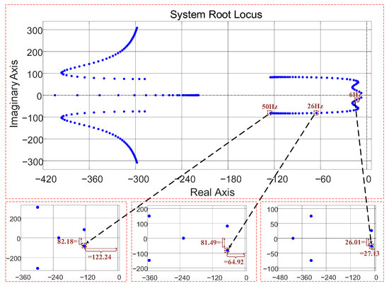
Figure 1.
Pole Location Distribution Plot.
The variables zn and pn represent the zeros and poles of (s). For ωinv0 = 6 Hz, 35 Hz, and 50 Hz, the corresponding values of zn and pn of (s) are obtained as follows:
From the above expression and Figure 1, it can be observed that:
- Under all operating conditions, the motor remains asymptotically stable. Variations in the dominant poles p4,5 lead to differences in the natural frequency ωn and damping ratio ζ of the induction motor.
- As the operating frequency decreases, both the natural frequency and the damping ratio tend to decline.
- The presence of right-half-plane zeros za,b indicates that the induction motor exhibits non-minimum-phase behavior, which further reduces the damping ratio ζ and bandwidth.
- The decrease in operating frequency causes the zeros z1,2 to shift, effectively reducing damping, introducing additional overshoot, and leading to phase-margin erosion.
In summary, although the induction motor remains stable, its low-frequency stability margin is limited, increasing the risk of low-frequency oscillations. Moreover, as the damping ratio ζ decreases, the interaction-induced stability challenges between IMDs and the DC link become more pronounced [27]. Therefore, when the interactions between IMDs and the DC link are considered, the overall system stability and robustness are further weakened, diverging from conclusions drawn from motor-only modeling and analysis.
3. DQ-Coordinate Input Impedance Model of PWM IMDs
The stator flux–oriented PWM IMDs controller is shown in Figure 2. In the figure, (s) and (s) are the dq-axis current regulators; (s) denotes the speed regulator (PI controller); (s), (s), and (s) represent the sampling delay functions for the dq-axis currents and speed. Dd and Dq are the PWM modulation functions.
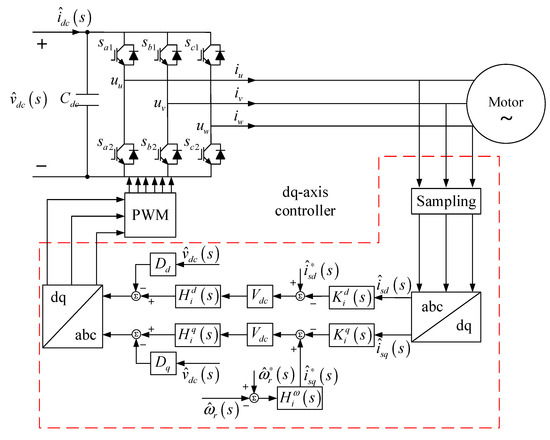
Figure 2.
Stator Flux-Oriented PWM IMD Controller.
The PWM IMDs controller comprises an inner current loop and an outer speed loop. The d-axis flux control loop solely regulates the stator flux, whereas the q-axis loop is responsible for torque control. In the induction motor’s multivariable transfer function, the dynamic relative gain array (DRGA) of Gs(s) reveals that the coupling elements (s) (i≠j) are significantly smaller than the diagonal elements (s). Therefore, their impact on the system’s dynamic characteristics can be regarded as a second-order perturbation.
During speed regulation below the fundamental frequency, the control system maintains a constant stator flux, while the q-axis loop regulates the speed. Therefore, the q-axis voltage is the primary variable for speed control. At the same time, speed perturbations primarily originate from . Moreover, Gs(s) indicates that the speed channel is decoupled from the d-axis. In addition, is considered an external mechanical disturbance with an effective bandwidth much lower than that of the electrical subsystem and can therefore be neglected.
3.1. D-Axis Control Small-Signal Equivalent Admittance Model
By employing stator flux–oriented control, the reference and feedback of isd inherently capture all flux information. Consequently, the d-axis can be regarded as an approximately independent SISO system, as illustrated in Figure 3.
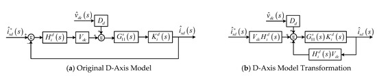
Figure 3.
D-Axis Control Small-Signal Model.
Figure 3a depicts the d-axis control loop. By accounting for both sampling delay and dead-time effects, the d-axis current sampling delay function is formulated. Its mathematical expression is given by:
Here, ωd denotes the cutoff frequency of the d-axis filter; ωtd denotes the sensor delay on the d-axis; Td denotes the d-axis current sampling interval; and Tdead denotes the dead-time duration.
Considering and for intuitive presentation, Figure 3a is transformed into Figure 3b, from which the closed-loop transfer functions are obtained as follows:
In (12), Td(s) reflects the close relationship between and in flux-oriented control. In the small-signal model, the small-signal component of Dd is denoted as . The relationship between and the PI controller is expressed as follows:
Based on Figure 3b, the small-signal equivalent admittance model for the d-axis control can be derived as:
In (14), is supplied by the controller defined in (13). Introducing Td(s) renders the complex closed-loop system equivalent to an admittance and indicates that the control action can alter its magnitude and phase. Thus, Td(s) transforms the closed-loop dynamics into an equivalent d-axis admittance model.
3.2. Q-Axis Control Small-Signal Equivalent Admittance Model
Similarly, the q-axis can be treated as an independent SISO system. The q-axis control adopts a dual-loop structure, consisting of an outer speed loop and an inner current loop. Neglecting low-order off-diagonal coupling terms, the transfer function relationship between speed and output current is illustrated in the schematic of Figure 4a.
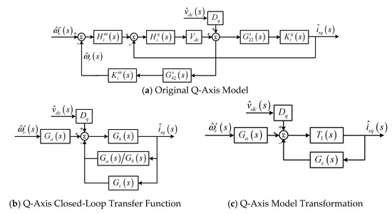
Figure 4.
Q-Axis Control Small-Signal Model.
The speed loop and current crossover configuration in Figure 4b is restructured into the parallel configuration shown in Figure 4c, which is further simplified into an admittance representation. A combined delay function accounting for sampling delay and dead-time effects is defined. Its mathematical expression is formulated as:
In the equation, ωq denotes the cutoff frequency of the q-axis filter; ωtq represents the q-axis sensor delay; Tq is the q-axis current sampling interval; and Tω is the q-axis speed sampling interval.
By applying an equivalent transformation, Figure 4a can be converted into Figure 4b, yielding Ga(s), Gb(s), and Gc(s) as follows:
The q-axis closed-loop transfer function is obtained from Figure 4c as follows:
Introducing Tq(s) renders the complex multi-loop closed-loop system equivalent to an admittance. Consequently, its impedance (s) can be interpreted as the equivalent impedance from q-axis voltage to current formed by coupling two loops, with the speed loop representing the dynamic response from q-axis voltage to speed. The equivalent impedances of the q-axis current inner loop and speed outer loop are given as follows:
The small-signal component of Dq is denoted as . The relationship between and the PI controllers of the current inner loop and the voltage outer loop is given as follows:
Based on Figure 4c and assuming , the following expression is obtained:
Equation (23) describes the dynamic model of PWM IMDs by accounting for electrical and mechanical parameters, including the modulation effect of speed variations, mechanical inertia, damping, and slip frequency. The magnitude and phase response of the q-axis impedance exhibit more pronounced electromechanical “source–load” coupling characteristics across the frequency domain.
3.3. Small-Signal Input Impedance Model of PWM IMDs
The inverter input is assumed to be supplied by a DC source with internal impedance [28]. This source can be a DC–DC converter or an AC–AC converter (rectifier). The corresponding small-signal equivalent circuit is shown in Figure 5. The red impedance in Figure 5 corresponds to the model obtained along the dq axis. Under DC-link small-signal perturbations, the inverter DC-link input current is expressed by:
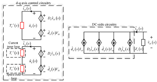
Figure 5.
Small-Signal Circuit Model.
Here, Isd and Isq denote the steady-state dq-axis stator currents, and represents the DC-link current of the PWM IMDs. Equation (24) captures the complete mapping of AC-link currents through the inverter to the DC link and converts the independent d- and q-axis SISO relationships into a single-variable relation on the DC link.
As shown in Figure 5, substituting (14) and (23) into (24) yields the PWM IMDs model driving the induction motor as follows:
Equation (25) defines the small-signal input impedance model of the PWM IMDs on the DC link. This model systematically captures the dynamic interactions between the DC link and the IMDs, with each term characterizing the coupling between the d- and q-axes, thereby offering a unified representation of the overall system behavior.
3.4. Small-Signal Equivalent Circuit of DC-Link Impedance Coupling
Based on (25), the equivalent DC circuit of the inverter connected to the DC link can be derived, as shown in Figure 6. Accordingly, the Nyquist Stability Criterion (NSC) can be applied to assess the interaction stability between the DC link and the inverter (IMDs).
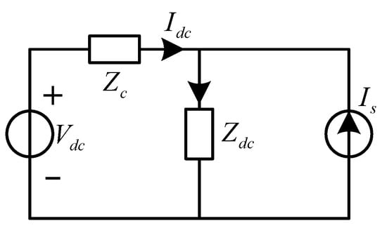
Figure 6.
Norton equivalent model.
Since IMDs utilize a current-controlled inverter, they can be equivalently represented as a current source Is in parallel with an input impedance Zdc(s) [29]. Consequently, the input current can be calculated as follows:
In this figure, vdc(s) represents the ideal DC-link voltage, which remains stable under inverter no-load conditions. Moreover, Is(s) also remains stable when the IMDs are fed by an ideal source, and Section 2.2 has demonstrated that 1/Zdc(s) is stable. Consequently, the overall system stability depends on the term 1/(1 + Zc(s)/Zdc(s)). The system stability can be assessed by examining whether the Nyquist plot of Zc(s)/Zdc(s) encircles the point (−1, j0).
4. Model Validation and Stability Analysis Under Various Operating Conditions
To validate the accuracy and effectiveness of the proposed model, this section presents experimental verification using a laboratory PWM IMDs platform and an induction motor, focusing on system stability under various motor operating conditions and their associated impacts.
The laboratory three-phase induction motor (IM) is mechanically loaded by a separately excited DC motor (SE-DC motor) acting as an equivalent load. The experimental setup, shown in Figure 7, integrates a power amplification module and an injection isolation transformer. The control system is implemented on a ZYNQ XC-7035 platform, and voltage and current sampling are performed using the high-speed A/D converter AD7606. The ZYNQ XC-7035 was sourced from Xilinx, San Jose, CA, USA, and the AD7606 was sourced from Analog Devices, Norwood, MA, USA. The parameters of the PWM IMDs used in the experiments are listed in Table 2.
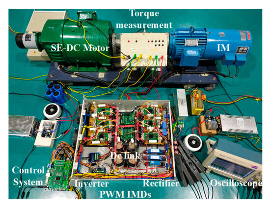
Figure 7.
Experimental prototype of the three-phase PWM IMDs with an IM coupled with a PMSM as a load.
Table 2.
Parameters of PWM IMDs in laboratory.
4.1. Induction Motor Operation in Quadrant I
From Figure 2, the DC-link impedance can be obtained from (27).
Here, R denotes the resistance between the DC link and the power source; Ldc represents the total source inductance; and Cdc denotes the shunt capacitance of the DC link. Under rated speed and torque conditions, the response of the PWM IMDs input impedance model is shown in Figure 8. In the figure, the red dashed line represents the simulated Zc(s), the blue solid line depicts the simulated input impedance Zdc(s) of the PWM IMDs under rated conditions, and the circle markers correspond to experimental measurements. The calculated results for PWM IMDs under rated conditions closely match the experimental measurements, thereby confirming the accuracy of the proposed impedance model.
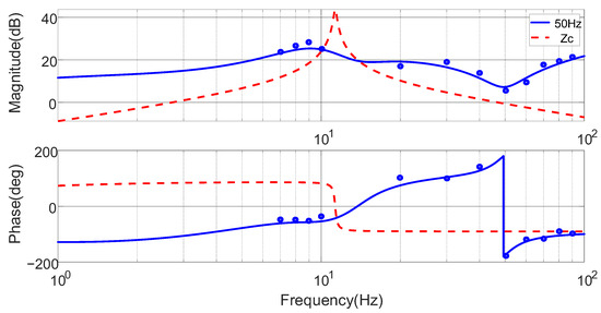
Figure 8.
Frequency responses for the sequence impedances of PWM IMDs and its experimental measurement results, under Motor Operating Condition I.
Figure 8 shows that Zc(s) behaves as an inductive impedance at low frequencies, transitioning to an RC characteristic at the natural frequency ωn. In contrast, Zdc(s) exhibits a negative-resistance-inductive (NRI, φ ∈ [−90°, −180°]) behavior in the low-frequency range. This phenomenon is primarily caused by dynamic stability variations resulting from the DC link feedback mechanism and nonlinear interactions between the converter and PWM IMDs within specific frequency ranges. According to the small-signal equivalent circuit (Figure 6), resonance may be excited at ωn, the natural frequency of Zc(s). Unlike typical series or parallel resonances confined to a single frequency, this resonance can occur across a range of frequencies, resulting in low-frequency oscillations of the DC-link current idc in PWM IMDs.
In contrast, Zdc(s) exhibits complex frequency-dependent behavior, with over fifty operating frequencies during motor speed regulation, each presenting distinct magnitude and phase characteristics. For clear and convenient analysis, the impedance model of Zdc(s) within the fundamental frequency range is divided into three segments: low-frequency (1–15 Hz), mid-frequency (16–30 Hz), and high-frequency (31–50 Hz). To facilitate clear and generalizable analysis, experimental tests were conducted at 8 Hz, 26 Hz, 37 Hz, and 48 Hz under Quadrant I operating conditions. Figure 9a–d presents the Bode plots of Zc(s) and Zdc(s) at the four corresponding frequencies.
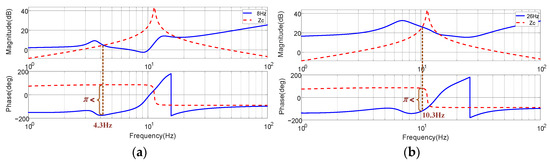
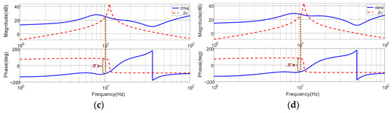
Figure 9.
Frequency responses for the sequence impedances of PWM IMDs and stability assessment, with Motor Operating Condition I. (a) 8 Hz, (b) 26 Hz, (c) 37 Hz, (d) 48 Hz.
From Figure 9a,b, it can be observed that the magnitude–frequency responses of Zdc(s) and Zc(s) intersect at an unstable point, where the phase difference at the intersection exceeds π. Under these conditions, when the inverter operates at 8 Hz, a low-frequency oscillation occurs at ƒosc = 4.3 Hz. Similarly, when operating at 26 Hz, a low-frequency oscillation appears at ƒosc = 10.3 Hz. In contrast, in Figure 9c,d, the phase difference at the magnitude-equal points is less than π, indicating system stability. Therefore, it is evident that the motor is more prone to instability when operating at low speeds under Quadrant I conditions. The Nyquist plots at 8 Hz, 26 Hz, 37 Hz, and 48 Hz under Quadrant I conditions are presented in Figure 10.
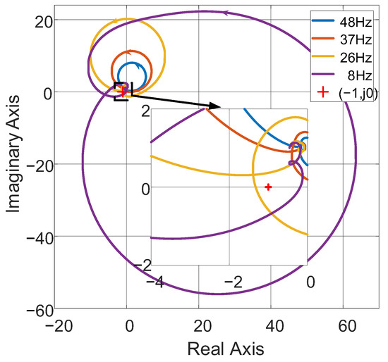
Figure 10.
Nyquist plots of impedance ratios Zc(s)/Zdc(s) for stability assessment with Motor Operating Condition I.
From Figure 10, the Nyquist plots at 8 Hz and 26 Hz encircle (−1, j0), indicating system instability according to the Nyquist criterion, whereas the plots at 37 Hz and 48 Hz do not encircle (−1, j0), indicating system stability. These conclusions agree with those obtained from the Bode plot analysis.
To analyze the impact of DC-link instability on PWM IMDs’ operation and to further validate the accuracy of the two aforementioned criteria, experiments were conducted at rated torque and an output frequency of 8 Hz. The variables ,
, , , and were measured and subjected to FFT analysis. The results are shown in Figure 11.
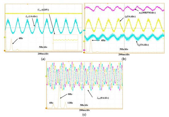
Figure 11.
Experimental waveforms of
, , , , and with Motor Operating Condition I. (a) and , (b) and , (c) .
As shown in Figure 11a, the inverter input current from the DC link exhibits a 4 Hz low-frequency oscillation, and the bus output voltage undergoes the same oscillatory behavior. The waveforms in Figure 11b indicate that the induction motor’s dq-domain currents also oscillate at 4 Hz, and the rotor speed fluctuates at the same frequency. Due to the DC-link current oscillations, the three-phase stator currents of the induction motor also exhibit a 4 Hz low-frequency oscillation. Additionally, when PWM IMDs operate at 8 Hz, SPWM modulation introduces interharmonic current components at 8 Hz ± 4 Hz, with the 12 Hz component corresponding to a super-synchronous (fundamental frequency) interharmonic. These interharmonic currents ultimately induce speed oscillations in the motor, creating an electromechanical resonance between the DC link and the induction motor. The oscillation frequency of 4 Hz observed in Figure 11c closely aligns with the theoretical value of 4.3 Hz obtained from Figure 9.
4.2. Induction Motor Operation in Quadrant IV
High-power PWM IMDs frequently operate across multiple quadrants, with electrified railway traction and port quay cranes (STS) being the most representative applications. In particular, port STS systems often switch frequently between Quadrant I and Quadrant IV operation. In Quadrant IV, PWM IMDs operate in an energy-regeneration mode. In the experiments, a DC motor was configured to operate as a generator to drive the induction motor, thereby emulating actual Quadrant IV operating conditions. Similarly, operating frequencies of 5 Hz, 20 Hz, 34 Hz, and 47 Hz were selected for Quadrant IV tests, all at rated torque. Figure 12 presents the Bode plots of Zdc(s).
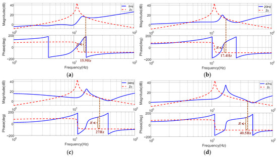
Figure 12.
Frequency responses for the sequence impedances of PWM IMDs and stability assessment, with Motor Operating Condition IV. (a) 7 Hz, (b) 24 Hz, (c) 34 Hz, (d) 47 Hz.
From Figure 12, the magnitude plots of Zdc(s) and Zc(s) intersect at 15.9 Hz, 17.4 Hz, 27 Hz, and 40.5 Hz, with phase differences exceeding 180°, indicating that their coupling induces instability. This instability arises because, in Quadrant IV operation, the PWM IMDs exhibit negative rotor speed ωr < 0, ωinv < 0, and s < 0, resulting in mechanical loads that provide negative damping. Figure 13 shows the corresponding Nyquist plots under these conditions.
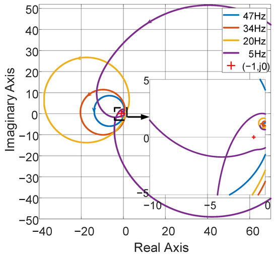
Figure 13.
Nyquist plots of impedance ratios Zc(s)/Zdc(s) for stability assessment with Motor Operating Condition IV.
From Figure 13, the Nyquist plots of the impedance ratios at all four speeds encircle (−1, j0), yielding stability conclusions consistent with those derived from the Bode plot analysis.
To evaluate the impact of DC link instability on PWM IMDs operating in Quadrant IV and to further validate the two aforementioned criteria, experiments were conducted under rated torque at an output frequency of 34 Hz. The variables , , , , and were measured and subjected to FFT analysis. The results are presented in Figure 14.
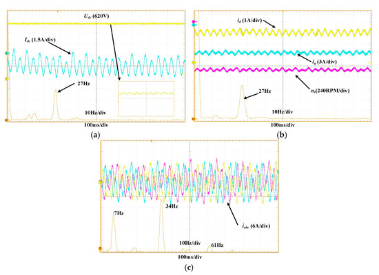
Figure 14.
Experimental waveforms of
, , , , and with Motor Operating Condition IV. (a) and , (b) and , (c) .
The waveforms in Figure 14 show that during Quadrant IV operation, idc is negative, indicating that the inverter feeds current back into the DC link. The DC-link current idc also exhibits a 27 Hz oscillation. Due to these DC link current fluctuations, the dq-axis currents exhibit oscillations at 27 Hz, which subsequently induce a 27 Hz low-frequency oscillation in the three-phase stator currents of the induction motor. When operating at 34 Hz, PWM IMDs generate interharmonic components in the stator currents due to SPWM modulation, specifically at 34 Hz ± 27 Hz, where the 61 Hz component corresponds to a super-synchronous interharmonic. These interharmonic currents ultimately induce a 27 Hz speed oscillation in the motor, similarly resulting in an electromechanical resonance between the DC link and the induction motor.
4.3. Induction Motor Operation Under Various Load Torques
4.3.1. Induction Motor Operation at 30% Load Torque
Experiments were conducted with the induction motor operating in Quadrant I at 30% of rated torque (4.5 N·m). Tests were performed at 7 Hz, 24 Hz, 34 Hz, and 44 Hz, and the results are shown in Figure 15.
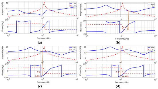
Figure 15.
Frequency responses for the sequence impedances of PWM IMDs and stability assessment, with Motor Operating Condition I and Operation at 30% Load Torque. (a) 7 Hz, (b) 24 Hz, (c) 34 Hz, (d) 44 Hz.
As shown in Figure 15a,b, the motor remains stable at 7 Hz and 24 Hz. However, Figure 15c,d reveals that Zdc(s) and Zc(s) intersect at ƒosc = 9.9 Hz and 10.4 Hz, respectively, with a phase difference exceeding π, indicating system instability.
Figure 16 presents the Nyquist plots of the induction motor operating at 30% of rated torque. Under 30% load, the Nyquist curves at 7 Hz and 24 Hz do not encircle (−1, j0), indicating system stability. In contrast, at 34 Hz and 44 Hz, the curves encircle (−1, j0), indicating system instability. These conclusions are consistent with those derived from the Bode plot analysis.
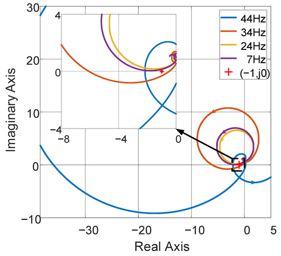
Figure 16.
Nyquist plots of impedance ratios Zc(s)/Zdc(s) for stability assessment with Motor Operating Condition I and Operation at 30% Load Torque.
To analyze the impact of DC-link instability on PWM IMDs operating at 30% load torque, experiments were conducted at 44 Hz. The variables , , , , and were measured and subjected to FFT analysis. The results are presented in Figure 17.
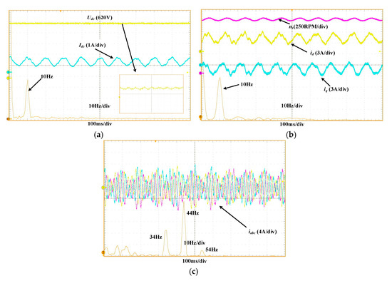
Figure 17.
Experimental waveforms of
, , , , and with Motor Operating Condition I and Operation at 30% Load Torque. (a) and , (b) and , (c) .
The waveforms in Figure 17 show that when the induction motor operates at 30% torque in Quadrant I, idc exhibits a 10 Hz oscillation. The dq-domain currents also oscillate at 10 Hz, inducing a 10 Hz low-frequency oscillation in the three-phase stator currents of the induction motor. Simultaneously, during 34 Hz operation of the PWM IMDs, SPWM modulation produces interharmonic components in the stator currents at 34 Hz ± 10 Hz, with the 44 Hz component corresponding to a super-synchronous interharmonic. These interharmonic currents ultimately cause a 10 Hz speed oscillation, leading to electromechanical resonance between the DC link and the induction motor.
4.3.2. Induction Motor Operation at 130% Load Torque
Experiments were conducted with the induction motor operating in Quadrant I at 130% of rated torque (19.4 N·m). To more comprehensively validate the results, tests were performed at 6 Hz, 18 Hz, 33 Hz, and 42 Hz. The outcomes are presented in Figure 18.
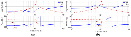
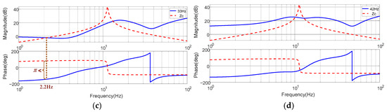
Figure 18.
Frequency responses for the sequence impedances of PWM IMDs and stability assessment, with Motor Operating Condition I and Operation at 130% Load Torque. (a) 6 Hz, (b) 18 Hz, (c) 33 Hz, (d) 42 Hz.
From Figure 18, it can be seen that under overload conditions, the dq-axis currents increase markedly, and Zdc(s) exhibits a stronger negative-impedance characteristic in the mid–low frequency range. Simultaneously, the higher load torque increases the slip and mechanical damping, shifting the system’s natural frequency toward the lower-frequency range. In Figure 18a–c, Zdc(s) and Zc(s) intersect in magnitude at ƒosc = 1.8 Hz, 10 Hz, and 2.2 Hz, respectively, with phase differences approaching or exceeding 180°, resulting in phase-margin loss or system instability.
The Nyquist plots at 130% load are shown in Figure 19. It can be observed that the Nyquist plots of the impedance ratios under heavy load at 6 Hz, 18 Hz, and 33 Hz encircle (–1, j0). In contrast, at 42 Hz, the plot does not encircle (−1, j0). These stability conclusions are consistent with those derived from the Bode plot analysis.
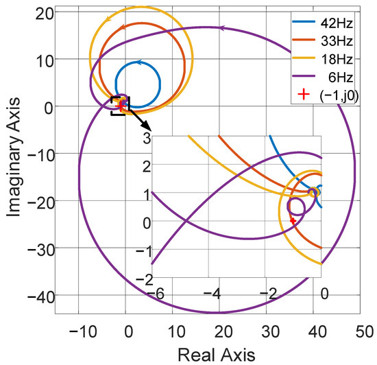
Figure 19.
Nyquist plots of impedance ratios Zc(s)/Zdc(s) for stability assessment with Motor Operating Condition I and Operation at 130% Load Torque.
To analyze the impact of DC-link instability on PWM IMDs operating at 30% load torque, experiments were conducted at 18 Hz. The variables , , , , and were measured and subjected to FFT analysis. The results are presented in Figure 20.
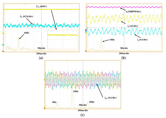
Figure 20.
Experimental waveforms of
, , , , and with Motor Operating Condition I and Operation at 130% Load Torque. (a) and , (b) and , (c) .
As shown in Figure 20, under 130% load operation in Quadrant I, idc exhibits a 10 Hz oscillation. The dq-domain currents also oscillate at 10 Hz, resulting in a 10 Hz low-frequency oscillation of the three-phase stator currents. When operating at 18 Hz, PWM IMDs produce interharmonic components due to SPWM modulation at 18 Hz ± 10 Hz, where the 28 Hz component constitutes a super-synchronous interharmonic relative to the 18 Hz fundamental. These interharmonic currents ultimately induce a 10 Hz oscillation in the rotor speed, leading to electromechanical resonance between the DC link and the induction motor.
4.4. Effects of PI Controller Bandwidth Tuning on the System and Its Design Methodology
To investigate the impact of the PI controller bandwidth on the input impedance characteristics and DC-link interaction stability of the system, this study experimentally adjusts the bandwidths of the d-axis and q-axis current loop controllers separately and analyzes the corresponding frequency responses. Specifically, by modifying the PI controller parameters to vary the open-loop gain crossover frequency, i.e., the control bandwidth, we obtained the system’s input impedance Bode plots under different bandwidth settings, as shown in Figure 21a for the d-axis and Figure 21b for the q-axis.
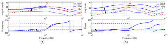
Figure 21.
The Bode plots of input impedance under different current PI controller bandwidths: (a) d-axis; (b) q-axis.
The experimental results show that when the bandwidth is set too low (e.g., <300 Hz), the system exhibits stronger capacitive behavior at low frequencies, causing the ZDC(s) to present a negative impedance characteristic and significantly reducing the system’s stability margin. Under such conditions, oscillations are likely to occur in the low-frequency range (e.g., 1–5 Hz), adversely affecting the reliability of the drive system. On the other hand, when the bandwidth is set too high (e.g., >1 kHz), although the current response speed improves, it also introduces negative effects. Specifically, the magnitude of ZDC(s) increases noticeably in the mid-frequency range, while the phase decreases further, leading to unfavorable stability conditions. This makes the system more susceptible to gain overlap and insufficient phase margin under high-frequency disturbances. Based on the above analysis, the overall impedance performance is most favorable when the d-axis and q-axis controller bandwidths are set within the range of approximately 800 Hz to 1 kHz. This range achieves a good balance between dynamic performance and stability. Accordingly, this study proposes a PI controller bandwidth design guideline: bandwidth should neither be set too low nor too high. Instead, it should be appropriately selected based on the inverter switching frequency, motor parameters, and desired dynamic performance to ensure robust stability across the full operating range.
5. Conclusions
This paper considers the coupling effects between the DC link and inverter control and develops a frequency-domain input impedance model for dual-loop speed-controlled PWM IMDs. From the perspective of the “source–load” impedance ratio, stability issues and their influencing factors in the interaction between the PWM IMDs and the DC link are analyzed using Bode plots and the Nyquist stability criterion (NSC). The main conclusions are summarized as follows:
- The induction motor’s MIMO state-space transfer function is inherently stable. However, it possesses a pair of small conjugate dominant poles which, under coupling conditions and decreasing PWM IMDs output frequency, can readily induce low-frequency oscillations in the PWM IMDs.
- By employing stator flux–oriented control, the MIMO model can be reduced to two SISO loops along the d- and q-axes, enabling direct construction of the PWM IMDs input impedance model Zdc(s) in the dq reference frame. Integrate the control system and the induction motor into the impedance model Zdc(s).
- During speed adjustment in PWM IMDs, low-frequency oscillations are more likely to occur, whereas stability improves as operating frequency increases. Under Quadrant IV operation, low-frequency oscillations become more severe, and new oscillatory modes appear in the mid-frequency range. Additionally, light-load conditions further increase the likelihood of oscillatory behavior.
- The low-frequency oscillations on the DC link, arising from the coupling with PWM IMDs, propagate into the induction motor, causing its three-phase currents and rotor speed to oscillate at the same frequency and triggering electromechanical resonance.
- During electromechanical resonance, the induction motor exhibits one sub-synchronous interharmonic and one super-synchronous interharmonic current, while the DC link experiences low-frequency current oscillations; this current is injected into the inverter under Quadrant I conditions and fed back into the bus under Quadrant IV conditions.
- By tuning the bandwidth of the current PI controllers, the impact on input impedance characteristics and DC-link interaction stability was systematically analyzed. It is recommended that the controller bandwidth be set within the range of 800 Hz to 1 kHz to achieve a balance between dynamic performance and stability margin.
Unlike existing studies that either focus on open-loop models or treat motor dynamics and control systems in isolation, this work proposes a unified impedance modeling framework that integrates motor dynamics, closed-loop control, and motor–converter coupling. This comprehensive approach enables accurate characterization of DC-link interaction stability under diverse operating conditions, which has not been systematically addressed in prior literature. The proposed model establishes a solid foundation for future stability analysis of multi-converter DC systems.
In future research, efforts will be made to validate the proposed impedance model in real industrial environments. The overall DC-link impedance model will be further extended to incorporate the grid-side converter, enhancing its physical relevance and capturing grid-connected effects. In addition, stability assessment under complex load conditions will be investigated, and advanced control strategies such as impedance shaping will be introduced to improve system robustness.
Author Contributions
D.Y. designed the study, collected the data, and revised and polished the manuscript. Z.K. wrote the manuscript, conducted the literature review, and prepared the figures. Y.W. was responsible for data collection and data analysis. W.R. prepared the figures and performed literature retrieval. Y.Y. also contributed to figure preparation and literature review. K.X. provided resources and supervised the overall process. All authors have read and agreed to the published version of the manuscript.
Funding
This research received no external funding. The APC was funded by the authors themselves.
Data Availability Statement
The data that support the findings of this study are not publicly available due to confidentiality restrictions but can be obtained from the corresponding author upon reasonable request. The data will be provided after approval.
Conflicts of Interest
The authors declare no conflict of interest.
References
- Singh, S.; Gautam, A.R.; Fulwani, D. Constant power loads and their effects in DC distributed power systems: A review. Renew. Sustain. Energy Rev. 2017, 72, 407–421. [Google Scholar] [CrossRef]
- Li, Q.; Dong, X.; Yan, M.; Cheng, Z.; Wang, Y. Research on the Hybrid Wind–Solar–Energy Storage AC/DC Microgrid System and Its Stability during Smooth State Transitions. Energies 2023, 16, 7930. [Google Scholar] [CrossRef]
- Abdelwanis, M.I.; Elmezain, M.I. A comprehensive review of hybrid AC/DC networks: Insights into system planning, energy management, control, and protection. Neural Comput. Appl. 2024, 36, 17961–17977. [Google Scholar] [CrossRef]
- Lan, J.; Chen, W.; Shu, L. A hybrid submodule three-phase multiplexing arm modular multilevel converter with wide operation range and DC-fault blocking capability. IEEE J. Emerg. Sel. Top. Power Electron. 2023, 11, 4148–4163. [Google Scholar] [CrossRef]
- He, B.; Chen, W.; Li, X.; Shu, L.; Zou, Z.; Liu, F. Unified frequency-domain small-signal stability analysis for interconnected converter systems. IEEE J. Emerg. Sel. Top. Power Electron. 2022, 11, 532–544. [Google Scholar] [CrossRef]
- Wen, B.; Dong, D.; Boroyevich, D.; Burgos, R.; Mattavelli, P.; Shen, Z. Impedance-based analysis of grid-synchronization stability for three-phase paralleled converters. IEEE Trans. Power Electron. 2015, 31, 26–38. [Google Scholar] [CrossRef]
- Fachini, F.; de Castro, M.; Bogodorova, T.; Vanfretti, L. Modeling of Induction Motors and Variable Speed Drives for Multi-Domain System Simulations Using Modelica and the OpenIPSL Library. Electronics 2024, 13, 1614. [Google Scholar] [CrossRef]
- Yang, D.; Jiang, J. Impedance modelling and stability assessment for grid-connected dual-PWM adjustable speed drives with motor torque oscillations. IET Electr. Power Appl. 2022, 16, 828–843. [Google Scholar] [CrossRef]
- Zhao, E.; Han, Y.; Lin, X.; Yang, P.; Blaabjerg, F.; Zalhaf, A.S. Impedance characteristics investigation and oscillation stability analysis for two-stage PV inverter under weak grid condition. Electr. Power Syst. Res. 2022, 209, 108053. [Google Scholar] [CrossRef]
- Zhang, H.; Harnefors, L.; Wang, X.; Hasler, J.P.; Östlund, S.; Danielsson, C.; Gong, H. Loop-at-a-time stability analysis for grid-connected voltage-source converters. IEEE J. Emerg. Sel. Top. Power Electron. 2020, 9, 5807–5821. [Google Scholar] [CrossRef]
- Zong, H.; Zhang, C.; Cai, X.; Molinas, M. A Multilayer Eigen-Sensitivity Method Using Loop Gain Model for Oscillation Diagnosis of Converter-Based System. arXiv 2024, arXiv:2402.12057. [Google Scholar]
- Yang, D.; Zhou, Z.; Liu, Y.; Jiang, J. Modeling of dual-PWM adjustable speed drives for characterizing input interharmonics due to torque oscillations. IEEE J. Emerg. Sel. Top. Power Electron. 2020, 9, 1565–1577. [Google Scholar] [CrossRef]
- Nian, H.; Yang, J.; Hu, B.; Jiao, Y.; Xu, Y.; Li, M. Stability analysis and impedance reshaping method for DC resonance in VSCs-based power system. IEEE Trans. Energy Convers. 2021, 36, 3344–3354. [Google Scholar] [CrossRef]
- Tu, C.; Gao, J.; Xiao, F.; Guo, Q.; Jiang, F. Stability analysis of the grid-connected inverter considering the asymmetric positive-feedback loops introduced by the PLL in weak grids. IEEE Trans. Ind. Electron. 2021, 69, 5793–5802. [Google Scholar] [CrossRef]
- Li, J.; Li, Y.; Zhang, X.; Xu, Z.; Du, Z. Design-oriented DC-side stability analysis of VSC-HVDC systems based on dominant frequency analysis. Int. J. Electr. Power Energy Syst. 2021, 149, 109060. [Google Scholar] [CrossRef]
- Shah, S.; Parsa, L. Sequence domain transfer matrix model of three-phase voltage source converters. In Proceedings of the 2016 IEEE Power and Energy Society General Meeting (PESGM), Boston, MA, USA, 17–21 July 2016; IEEE: Piscataway, NJ, USA, 2016; pp. 1–5. [Google Scholar]
- He, B.; Chen, W.; Ruan, X.; Zhang, X.; Zou, Z.; Cao, W. A generic small-signal stability criterion of DC distribution power system: Bus node impedance criterion (BNIC). IEEE Trans. Power Electron. 2021, 37, 6116–6131. [Google Scholar] [CrossRef]
- Yang, D.; Zhang, X.; Li, Y.; Chen, M. MIMO sequence impedance modeling and stability assessment for grid-connected dual-PWM adjustable-speed drives. Int. J. Electr. Power Energy Syst. 2025, 169, 108876. [Google Scholar] [CrossRef]
- Guha, A.; Narayanan, G. Small-signal stability analysis of an open-loop induction motor drive including the effect of inverter deadtime. IEEE Trans. Ind. Appl. 2015, 52, 242–253. [Google Scholar] [CrossRef]
- Zhang, S.; Kang, J.; Yuan, J. Analysis and suppression of oscillation in V/F controlled induction motor drive systems. IEEE Trans. Transp. Electrif. 2021, 8, 1566–1574. [Google Scholar] [CrossRef]
- Xu, L.; Xin, H.; Huang, L.; Yuan, H.; Ju, P.; Wu, D. Symmetric admittance modeling for stability analysis of grid-connected converters. IEEE Trans. Energy Convers. 2019, 35, 434–444. [Google Scholar] [CrossRef]
- Zou, Z.; Tang, J.; Wang, X.; Wang, Z.; Chen, W.; Buticchi, G.; Liserre, M. Modeling and control of a two-bus system with grid-forming and grid-following converters. IEEE J. Emerg. Sel. Top. Power Electron. 2022, 10, 7133–7149. [Google Scholar] [CrossRef]
- Fan, L.; Miao, Z. Admittance-based stability analysis: Bode plots, nyquist diagrams or eigenvalue analysis? IEEE Trans. Power Syst. 2020, 35, 3312–3315. [Google Scholar] [CrossRef]
- Pan, P.; Chen, W.; Shu, L.; Mu, H.; Zhang, K.; Zhu, M.; Deng, F. An impedance-based stability assessment methodology for DC distribution power system with multivoltage levels. IEEE Trans. Power Electron. 2019, 35, 4033–4047. [Google Scholar] [CrossRef]
- Umetani, Y.; Yoshida, K. Resolved Motion Rate Control of Space Manipulators with Generalized Jacobian Matrix. Doctoral Dissertation, Tohoku University, Sendai, Japan, 1989. [Google Scholar]
- Chen, C.T. Linear System Theory and Design; Saunders College Publishing: Philadelphia, PA, USA, 1984. [Google Scholar]
- Paraskevopoulos, P.N. Modern Control Engineering; CRC Press: Boca Raton, FL, USA, 2017. [Google Scholar]
- Gao, F.; Bozhko, S. Modeling and impedance analysis of a single DC bus-based multiple-source multiple-load electrical power system. IEEE Trans. Transp. Electrif. 2016, 2, 335–346. [Google Scholar] [CrossRef]
- Liu, Y.; Zhou, X.; Yu, H.; Hong, L.; Xia, H.; Yin, H.; Chen, Y.; Zhou, L.; Wu, W. Sequence impedance modeling and stability assessment for load converters in weak grids. IEEE Trans. Ind. Electron. 2020, 68, 4056–4067. [Google Scholar] [CrossRef]
Disclaimer/Publisher’s Note: The statements, opinions and data contained in all publications are solely those of the individual author(s) and contributor(s) and not of MDPI and/or the editor(s). MDPI and/or the editor(s) disclaim responsibility for any injury to people or property resulting from any ideas, methods, instructions or products referred to in the content. |
© 2025 by the authors. Licensee MDPI, Basel, Switzerland. This article is an open access article distributed under the terms and conditions of the Creative Commons Attribution (CC BY) license (https://creativecommons.org/licenses/by/4.0/).