
Ensemble Learning-Based Metamodel for Enhanced Surface Roughness Prediction in Polymeric Machining

 , ,
, , 
Abstract
1. Introduction
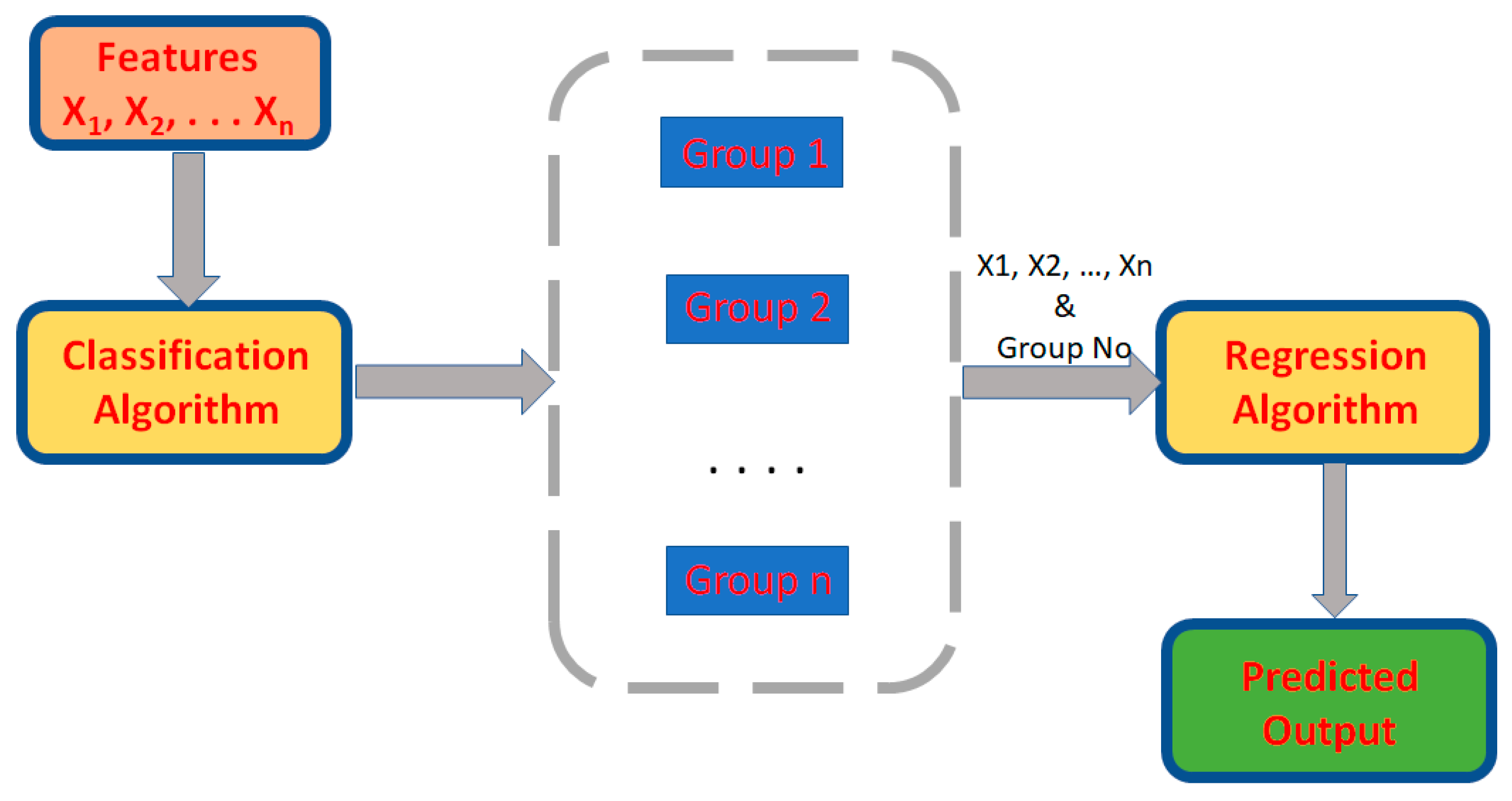
2. Model Development Methodology in Detail
Cross Validation Method (k-Fold Method)
3. Verification of the Proposed Model Development
3.1. Materials and Experiments
3.2. Meta-Based Model
3.3. Results and Discussion
3.3.1. Quantile Distribution Method
3.3.2. Correlation Analysis
3.3.3. Performance of Meta-Based Models
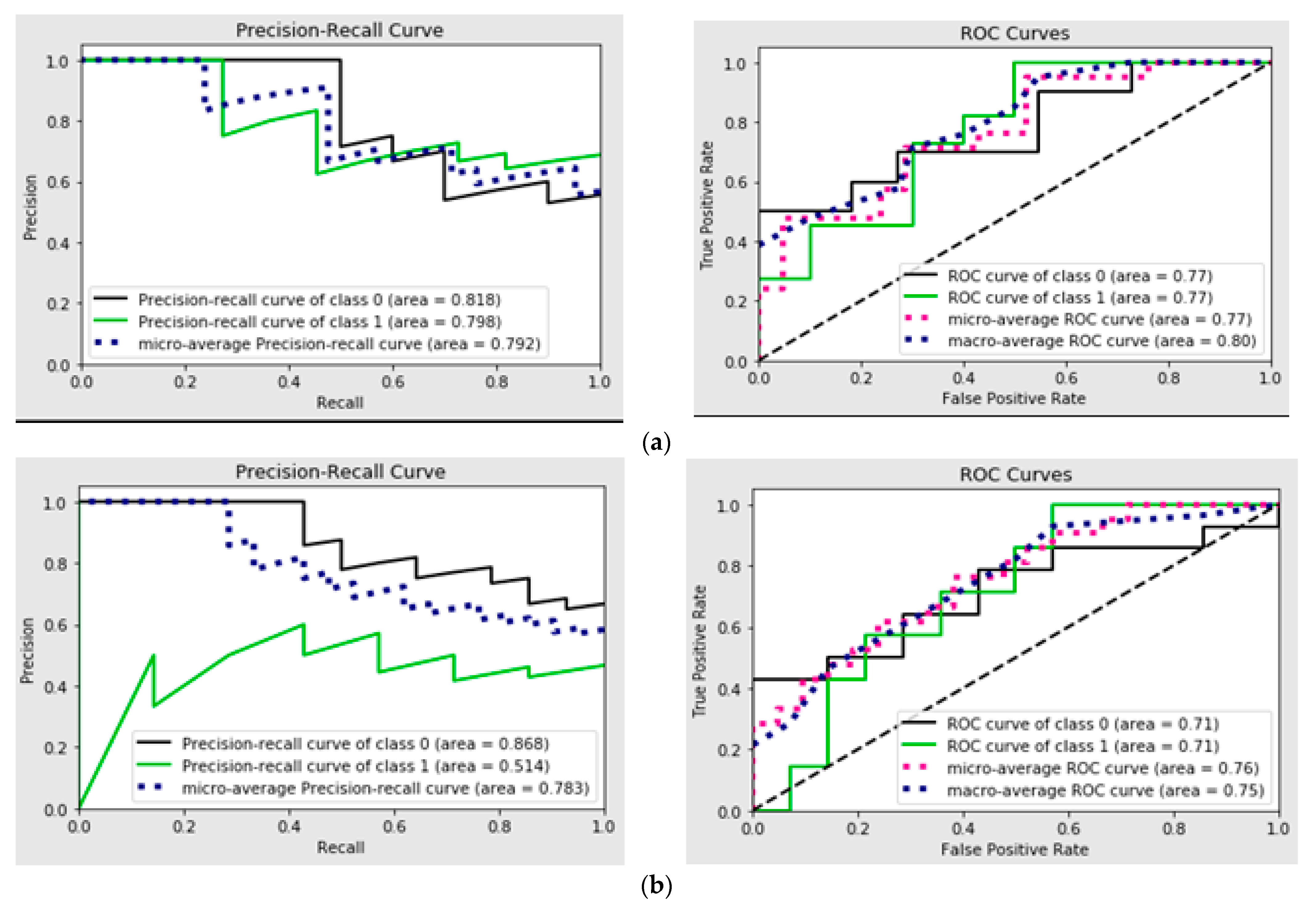
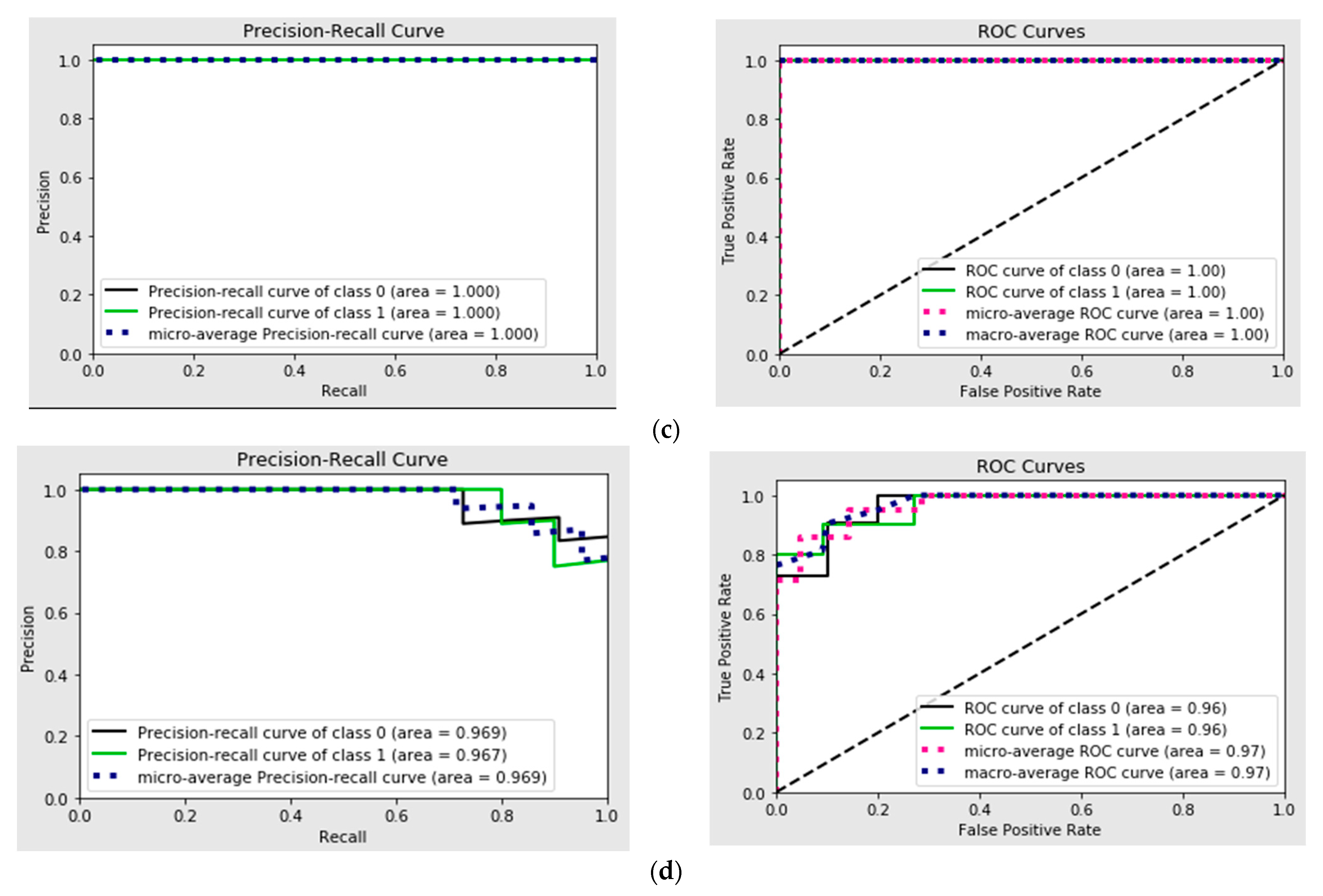
3.3.4. Receiver Operating Characteristic (ROC) Curve Analysis
3.3.5. Limitation of the Study
4. Conclusions and Further Improvement
Author Contributions
Funding
Data Availability Statement
Conflicts of Interest
References
- Elango, S.; Natarajan, E.; Varadaraju, K.; Gnanamuthu, E.M.A.; Durairaj, R.; Mohanraj, K.; Osman, M.A. Extreme gradient boosting regressor solution for defy in drilling of materials. Adv. Mater. Sci. Eng. 2022, 2022. [Google Scholar] [CrossRef]
- Natarajan, E.; Fiorna, V.; Abdulaziz, A.-T.A.; Elango, S.; Abraham, G.E.M.; Saruchi, S.A.B. Characteristics of Machining Data and Machine Learning Models—Case Study. IET Conf. Proc. 2023, 23, 117–122. [Google Scholar] [CrossRef]
- Li, P.; Chang, Z. Accurate modeling of working normal rake angles and working inclination angles of active cutting edges and application in cutting force prediction. Micromachines 2021, 12, 1207. [Google Scholar] [CrossRef] [PubMed]
- Dörr, M.; Ott, L.; Matthiesen, S.; Gwosch, T. Prediction of tool forces in manual grinding using consumer-grade sensors and machine learning. Sensors 2021, 21, 7147. [Google Scholar] [CrossRef]
- Chacón, J.L.F.; de Barrena, T.F.; García, A.; de Buruaga, M.S.; Badiola, X.; Vicente, J. A novel machine learning-based methodology for tool wear prediction using acoustic emission signals. Sensors 2021, 21, 5984. [Google Scholar] [CrossRef]
- Xiao, Q.; Li, C.; Tang, Y.; Chen, X. Energy Efficiency Modeling for Configuration-Dependent Machining via Machine Learning: A Comparative Study. IEEE Trans. Autom. Sci. Eng. 2021, 18, 717–730. [Google Scholar] [CrossRef]
- Kundu, P.; Luo, X.; Qin, Y. Automatic Identification of Most Suitable Sensors and Health Indicators for Cutting Tool Wear Prediction in Smart Manufacturing Systems. In Proceedings of the 2021 26th International Conference on Automation and Computing (ICAC), Portsmouth, UK, 2–4 September 2021. [Google Scholar]
- Li, J.; Lu, J.; Chen, C.; Ma, J.; Liao, X. Tool wear state prediction based on feature-based transfer learning. Int. J. Adv. Manuf. Technol. 2021, 113, 3283–3301. [Google Scholar] [CrossRef]
- Varghese, A.; Kulkarni, V.; Joshi, S.S. Tool life stage prediction in micro-milling from force signal analysis using machine learning methods. J. Manuf. Sci. Eng. Trans. ASME 2021, 143, 054501. [Google Scholar] [CrossRef]
- Zhang, H. Tool Cutting Force Prediction Model Based on ALO-ELM Algorithm. Comput. Intell. Neurosci. 2022, 2022, 1486205. [Google Scholar] [CrossRef]
- Bonci, A.; Di Biase, A.; Dragoni, A.F.; Longhi, S.; Sernani, P.; Zega, A. Machine learning for monitoring and predictive maintenance of cutting tool wear for clean-cut machining machines. In Proceedings of the 2022 IEEE 27th International Conference on Emerging Technologies and Factory Automation (ETFA), Stuttgart, Germany, 6–9 September 2022. [Google Scholar] [CrossRef]
- Malagi, R.R.; Barreto, R.; Chougula, S.R. Neural Network Based Model for Estimating Cutting Force During Machining of Ti-6Al-4V Alloy. J. Future Sustain. 2022, 2, 23–32. [Google Scholar] [CrossRef]
- Das, A.; Das, S.R.; Panda, J.P.; Dey, A.; Gajrani, K.K.; Somani, N.; Gupta, N.K. Machine learning-based modeling and optimization in hard turning of AISI d6 steel with advanced altisin-coated carbide inserts to predict surface roughness and other machining characteristics. Surf. Rev. Lett. 2022, 29, 2250137. [Google Scholar] [CrossRef]
- Guo, L.; Yu, Y.; Gao, H.; Feng, T.; Liu, Y. Online Remaining Useful Life Prediction of Milling Cutters Based on Multisource Data and Feature Learning. IEEE Trans. Ind. Inform. 2022, 18, 5199–5208. [Google Scholar] [CrossRef]
- Deng, C.; Tang, J.; Miao, J.; Zhao, Y.; Chen, X.; Lu, S. Efficient stability prediction of milling process with arbitrary tool-holder combinations based on transfer learning. J. Intell. Manuf. 2023, 34, 2263–2279. [Google Scholar] [CrossRef]
- Gao, S.; Duan, X.; Zhu, K.; Zhang, Y. Generic Cutting Force Modeling with Comprehensively Considering Tool Edge Radius, Tool Flank Wear and Tool Runout in Micro-End Milling. Micromachines 2022, 13, 1805. [Google Scholar] [CrossRef] [PubMed]
- Wang, R.; Zhao, M.; Mao, J.; Liang, S.Y. Force Prediction and Material Removal Mechanism Analysis of Milling SiCp/2009Al. Micromachines 2022, 13, 1687. [Google Scholar] [CrossRef]
- Kumar, V.; Dubey, V.; Sharma, A.K. Comparative analysis of different machine learning algorithms in prediction of cutting force using hybrid nanofluid enriched cutting fluid in turning operation. Mater. Today Proc. 2023, Advance online publication. [Google Scholar] [CrossRef]
- Liu, M.; Xie, H.; Pan, W.; Ding, S.; Li, G. Prediction of Cutting Force via Machine Learning: State of the Art, Challenges and Potentials; Springer: Berlin/Heidelberg, Germany, 2023. [Google Scholar] [CrossRef]
- Makhfi, S.; Dorbane, A.; Harrou, F.; Sun, Y. Prediction of Cutting Forces in Hard Turning Process Using Machine Learning Methods: A Case Study. J. Mater. Eng. Perform. 2023, 33, 9095–9111. [Google Scholar] [CrossRef]
- Ho, Q.N.T.; Do, T.T.; Minh, P.S. Studying the Factors Affecting Tool Vibration and Surface Quality during Turning through 3D Cutting Simulation and Machine Learning Model. Micromachines 2023, 14, 1025. [Google Scholar] [CrossRef]
- Liu, P.; Lou, S.; Shen, H.; Wang, M. Machine Learning for Prediction of Energy Consumption and Broken Force in the Chopping Process of Maize Straw. Agronomy 2023, 13, 3030. [Google Scholar] [CrossRef]
- Soori, M.; Arezoo, B.; Dastres, R. Machine learning and artificial intelligence in CNC machine tools, A review. Sustain. Manuf. Serv. Econ. 2023, 2, 100009. [Google Scholar] [CrossRef]
- Kathmore, P.; Bachchhav, B.; Nandi, S.; Salunkhe, S.; Chandrakumar, P.; Nasr, E.A.; Kamrani, A. Prediction of Thrust Force and Torque for High-Speed Drilling of AL6061 with TMPTO-Based Bio-Lubricants Using Machine Learning. Lubricants 2023, 11, 356. [Google Scholar] [CrossRef]
- Lee, S.; Jo, W.; Kim, H.; Koo, J.; Kim, D. Deep learning-based cutting force prediction for machining process using monitoring data. Pattern Anal. Appl. 2023, 26, 1013–1025. [Google Scholar] [CrossRef]
- Djellouli, K.; Haddouche, K.; Belarbi, M.; Aich, Z. Prediction of the cutting tool wear during dry hard turning of AISI D2 steel by using models based on Learning process and GA polyfit. J. Eng. Exact Sci. 2023, 9, 18297. [Google Scholar] [CrossRef]
- Yurtkuran, H.; Korkmaz, M.E.; Gupta, M.K.; Yılmaz, H.; Günay, M.; Vashishtha, G. Prediction of power consumption and its signals in sustainable turning of PH13-8Mo steel with different machine learning models. Int. J. Adv. Manuf. Technol. 2024, 133, 2171–2188. [Google Scholar] [CrossRef]
- Nair, V.S.; Rameshkumar, K.; Saravanamurugan, S. Chatter Identification in Milling of Titanium Alloy Using Machine Learning Approaches with Non-Linear Features of Cutting Force and Vibration Signatures. Int. J. Progn. Health Manag. 2024, 15, 1–15. [Google Scholar] [CrossRef]
- Sharma, M.K.; Alkhazaleh, H.A.; Askar, S.; Haroon, N.H.; Almufti, S.M.; Al Nasar, M.R. FEM-supported machine learning for residual stress and cutting force analysis in micro end milling of aluminum alloys. Int. J. Mech. Mater. Des. 2024, 20, 1077–1098. [Google Scholar] [CrossRef]
- Pashmforoush, F.; Araghizad, A.E.; Budak, E. Physics-informed tool wear prediction in turning process: A thermo-mechanical wear-included force model integrated with machine learning. J. Manuf. Syst. 2024, 77, 266–283. [Google Scholar] [CrossRef]
- Kouguchi, J.; Tajima, S.; Yoshioka, H. Machine-Learning-Based Model Parameter Identification for Cutting Force Estimation. Int. J. Autom. Technol. 2024, 18, 26–38. [Google Scholar] [CrossRef]
- Gross, D.; Spieker, H.; Gotlieb, A.; Knoblauch, R.; Elmansori, M. Efficient Milling Quality Prediction with Explainable Machine Learning. arXiv 2024, arXiv:2409.10203. [Google Scholar] [CrossRef]
- Reeber, T.; Wolf, J.; Möhring, H.C. A Data-Driven Approach for Cutting Force Prediction in FEM Machining Simulations Using Gradient Boosted Machines. J. Manuf. Mater. Process. 2024, 8, 107. [Google Scholar] [CrossRef]
- Colantonio, L.; Equeter, L.; Dehombreux, P.; Ducobu, F. Confidence Interval Estimation for Cutting Tool Wear Prediction in Turning Using Bootstrap-Based Artificial Neural Networks. Sensors 2024, 24, 3432. [Google Scholar] [CrossRef] [PubMed]
- Kim, K.; Islam, M.A.; Lih, S.-S.; Jang, J.-E. Machine learning design of nonlinear elastomeric springs fabricated via additive manufacturing. Addit. Manuf. 2023, 59, 103408. [Google Scholar]
- Ghaderi, R.; Mehrafrooz, B.; Ramamurty, U. Bayesian-based data-driven constitutive modeling of elastomers using experimental stress–strain data. Comput. Mech. 2022, 70, 387–401. [Google Scholar]
- Yan, Q.; Deng, S.; Zhao, H. Dual convolutional neural network model for predicting shape memory polymer performance using BigSMILES. Mater. Today Commun. 2023, 35, 105524. [Google Scholar] [CrossRef]
- Jin, L.; Wang, Z.; Liu, J.; Xu, Y. Optimization of high-performance epoxy resins using artificial neural networks. Polymers 2021, 13, 452. [Google Scholar] [CrossRef]
- Kuenneth, C.; Ramprasad, R. Data-driven polymer dielectrics design: Theory, descriptors, and predictions. Sci. Data 2020, 7, 122. [Google Scholar] [CrossRef]
- Shah, P.; Bhattacharyya, D.; Fang, Q. Machine learning-aided real-time prediction of melt pressure in PLA foam extrusion. Polym. Eng. Sci. 2022, 62, 3029–3042. [Google Scholar] [CrossRef]
- Vincent, A.M.; Jidesh, P. An improved hyperparameter optimization framework for AutoML systems using evolutionary algorithms. Sci. Rep. 2023, 13, 4737. [Google Scholar] [CrossRef]
- Aghaabbasi, M.; Ali, M.; Jasiński, M.; Leonowicz, Z.; Novák, T. On Hyperparameter Optimization of Machine Learning Methods Using a Bayesian Optimization Algorithm to Predict Work Travel Mode Choice. IEEE Access 2023, 11, 19762–19774. [Google Scholar] [CrossRef]
- Ali, Y.A.; Awwad, E.M.; Al-Razgan, M.; Maarouf, A. Hyperparameter Search for Machine Learning Algorithms for Optimizing the Computational Complexity. Processes 2023, 11, 349. [Google Scholar] [CrossRef]


| Purpose of the Research | Materials Involved | Algorithm Used | Year of Publication and Reference |
|---|---|---|---|
| An analytical model that predicts cutting force through working normal rake angle (WNRA) and working inclination angle (WIA) during turning operation. | GH 4169 (a nickel-based superalloy) | No ML algorithm was used as it is an Analytical model | 2021 [3] |
| An ML mode that predicts drill tool force through inputs from inertial measurement unit (IMU) and sensors. | Steel | Gaussian Process Regressor | 2021 [4] |
| An ML model that predicts tool flank wear through acoustic emission sensors during turning operation. | 19NiMoCr6 steel | Random forest regressor. The performance of the model was compared with ANN, SVM, KNN DT algorithms | 2021 [5] |
| An ML model that predicts the energy usage through cross sectional data, tool wear, and spindle motor life during machining. | Traditional algorithms such as Artificial Neural Networks, support vector regression, and Gaussian Process Regression and deep learning network | 2021 [6] | |
| To improve tool wear prediction accuracy, reduce computation time, model complexity, and enhance decision making in smart manufacturing systems. | HRC52 stainless steel | Random Forest Regression model for improving tool wear prediction accuracy | 2021 [7] |
| To accurately predict tool wear states during machining processes by utilizing historical machining data and improve product quality and operational efficiency. | TC18 titanium | Genetic algorithm for feature selection, maximum mean discrepancy for feature evaluation, and particle swarm-optimized vector for prediction | 2021 [8] |
| Predict tool life stages by using cutting force data to avoid catastrophic tool breakage during machining. | SS304 stainless steel | K-means clustering for machining data identification, principal component analysis for feature extraction, Random forest model for predicting tool life stage | 2021 [9] |
| To improve tool cutting prediction accuracy by using ALO-ELM algorithm. | 45 steel | Ant Lion Optimizer (ALO), Extreme Learning Machine (ELM), Backpropagation (BP) neural network, and support vector machine (SVM) | 2022 [10] |
| Develop learning algorithms for wear estimation, focusing on predictive maintenance of cutting tools. | Medium alloy steel, Hardox and C45 steel | SVM classifiers for wear classification, LSTM neural network for Remaining useful life (RUL) prediction and One-way Anova for feature selection | 2022 [11] |
| To improve cutting force prediction accuracy and optimize machining process for better outcomes. | Ti6AI4V | Artificial Neural Network (ANN) for cutting force prediction and Genetic Algorithm for optimization and estimation | 2022 [12] |
| Model and optimize hard turning of AISI D6 steel to reduce machine downtime and production costs. | AISI D6 steel | Polynomial regression (PR), Random forest (RF) regression, gradient boosted (GB) trees, and adaptive boosting (AB) based regression | 2022 [13] |
| To predict remaining useful life of milling cutters using multisource sensor data for accurate predictions. | C45 grade steel | Multiscale convolutional attention network (MSAN) for feature learning and Genetic Algorithm (GA) for parameter optimization | 2022 [14] |
| To predict milling stability efficiently using transfer learning in order to avoid chatter vibrations in milling processes. | Cemented carbide | Transfer learning | 2022 [15] |
| Develop cutting force model that can contribute to monitor machining process, optimizing cutting parameters, and ensuring machining quality. | AISI4340 alloy structural steel | No ML algorithm used as it is an Analytical model | 2022 [16] |
| To analyze milling force in SiCp/2009Al composites and study material removal mechanisms during milling. | Silicon carbide particle-reinforced aluminium matrix composites (SiCp/2009Al) | No ML algorithm used as it is an Analytical model | 2022 [17] |
| To monitor cutting tool degradation using neural networks and assess tool wear under varying cutting conditions. | AISI 304 steel | Random Forest Regressor (RF) model, Gradient Booster Regressor (GBR) model, and Extreme Gradient Booster Regressor (XGBoost) model | 2023 [18] |
| To review cutting force prediction methods and highlight machine learning potential in force prediction accuracy. | Fiber-reinforced ceramic matrix composites | Review of various machine learning models for cutting force prediction | 2023 [19] |
| To predict machining force components during hard turning of AISI 52100 bearing steel using machine learning models. | AISI 52100 bearing steel | Linear Regression (LR), Support vector regression, ensemble learning-based regression | 2023 [20] |
| To study the factors affecting vibration of the tool and surface quality of the workpiece during turning by applying simulation and machine learning model methods. | AA6061 aluminum | Neural network model | 2023 [21] |
| To reduce energy consumption in maize straw chopping and minimize breaking force during the chopping process by constructing a predictive model using machine learning algorithms. | Rind-Pith material: MATPLASTICKINEMATIC, density 1120 kg/m3 | Back-propagation (BP), Artificial Neural Network (ANN), Support vector regression | 2023 [22] |
| To review AI and ML applications in CNC machining. | Materials are not specified, as it is a review paper | Review of various Machine learning models used in CNC machining | 2023 [23] |
| To examine TMPTO-based lubricant effects n drilling performance, optimize thrust force and torque during high-speed drilling, and evaluate the biodegradable lube oils for cutting force prediction. | AA6061 aluminum | Random forest, Support vector machines | 2023 [24] |
| To predict cutting force in machining processes accurately, utilizing deep learning models. | Aluminum alloy | Deep learning, Long short-term memory (LSTM) model | 2023 [25] |
| Develop predictive models using machine learning techniques to predict flank wear during dry hard turning. | AISI D2 steel | Artificial Neural Network, support vector machine (SVM). Polynomial fit using Genetic Algorithm | 2023 [26] |
| To optimize energy consumption in machining process and apply machine learning techniques for predictive modeling. | PH13-8 Mo stainless steel | Linear regression, multilayer perceptron, gradient boost regression, and Adaboost regression | 2024 [27] |
| Develop machine learning models for chatter identification in milling. | Ti6AI4V alloy | Decision trees, support vector machines. | 2024 [28] |
| To characterize cutting force and residual stress using Bayesian machine learning framework for analysis and optimize machining parameters for surface integrity. | Aluminum alloys | Bayesian machine learning framework | 2024 [29] |
| To integrate physics-based models with machine learning to enhance production efficiency, production quality, and reduce manufacturing cost through improved monitoring | 1050 steel and Ti6AI4V alloy | Least-square boosting, Random forest, and support vector machine | 2024 [30] |
| Machine learning method for cutting force estimation and monitoring milling processes accurately. | Pre-hardened steel and A5052 aluminum alloy | Multilayer perceptron | 2024 [31] |
| Develop explainable machine learning models for accurate predictions. | 2071A aluminum alloy | Explainable Machine learning model | 2024 [32] |
| To capture non-linear behavior of material models and predict cutting forces efficiently. | Steel | Random forest, support vector machine, XGBoost, LightGBM | 2024 [33] |
| To monitor cutting tool degradation using neural networks and assess tool wear under varying cutting conditions. | C45 Steel | Neural Network | 2024 [34] |
| Material | Machining Parameter | Level | ||
|---|---|---|---|---|
| I | II | III | ||
| POM | Speed (Vc) (m/minute) | 90 | 135 | 180 |
| Feed (f) (mm/rev) | 0.1 | 0.3 | 0.5 | |
| Depth of cut (ap) (mm) | 0.5 | 1.0 | 1.5 | |
| PTFE | Speed (Vc) (m/minute) | 80 | 120 | 160 |
| Feed (f) (mm/rev) | 0.1 | 0.3 | 0.5 | |
| Depth of cut (ap) (mm) | 0.5 | 0.75 | 1.0 | |
| PEEK | Speed (Vc) (m/minute) | 95 | 125 | 155 |
| Feed (f) (mm/rev) | 0.2 | 0.4 | 0.6 | |
| Depth of cut (ap) (mm) | 0.25 | 0.5 | 0.75 | |
| PEEK/MWCNT composite | Speed (Vc) (m/minute) | 750 | 1500 | 2250 |
| Feed (f) (mm/rev) | 0.15 | 0.45 | 0.75 | |
| Depth of cut (ap) (mm) | 0.1 | 1.0 | 1.8 | |
| Material | Cutting Speed Vc (mm/min) | Feed Rate f (mm/rev) | Depth of Cut ap (mm) | Surface Roughness Ra (µm) |
|---|---|---|---|---|
| POM | 90 | 0.1 | 0.5 | 0.79 |
| 90 | 0.1 | 1.0 | 0.61 | |
| 90 | 0.1 | 1.5 | 0.56 | |
| 90 | 0.3 | 0.5 | 1.88 | |
| 90 | 0.3 | 1.0 | 1.78 | |
| 90 | 0.3 | 1.5 | 1.74 | |
| 90 | 0.5 | 0.5 | 1.67 | |
| 90 | 0.5 | 1.0 | 1.59 | |
| 135 | 0.5 | 1.5 | 1.65 | |
| 135 | 0.1 | 0.5 | 1.18 | |
| 135 | 0.1 | 1.5 | 0.84 | |
| 135 | 0.1 | 1.0 | 0.66 | |
| 135 | 0.3 | 0.5 | 1.60 | |
| 135 | 0.3 | 1.5 | 1.72 | |
| 135 | 0.3 | 1.0 | 1.66 | |
| 135 | 0.5 | 0.5 | 1.50 | |
| 135 | 0.5 | 1.5 | 1.80 | |
| 135 | 0.5 | 1.0 | 1.43 | |
| 180 | 0.1 | 0.5 | 1.19 | |
| 180 | 0.1 | 1.5 | 0.89 | |
| 180 | 0.1 | 1.0 | 0.67 | |
| 180 | 0.3 | 0.5 | 1.62 | |
| 180 | 0.3 | 1.5 | 1.65 | |
| 180 | 0.3 | 1.0 | 1.60 | |
| 180 | 0.5 | 0.5 | 1.42 | |
| 180 | 0.5 | 1.5 | 1.61 | |
| 180 | 0.5 | 1.0 | 1.59 | |
| Material | Cutting Speed Vc (mm/min) | Feed Rate f (mm/rev) | Depth of Cut ap (mm) | Surface Roughness Ra (µm) |
| PTFE | 120 | 0.3 | 1 | 2.26 |
| 120 | 0.3 | 0.75 | 2.67 | |
| 80 | 0.5 | 0.75 | 3.19 | |
| 160 | 0.3 | 0.75 | 2.69 | |
| 160 | 0.3 | 0.75 | 2.85 | |
| 160 | 0.3 | 0.75 | 2.46 | |
| 120 | 0.5 | 0.75 | 2.19 | |
| 80 | 0.3 | 0.5 | 1.76 | |
| 80 | 0.3 | 0.75 | 2.14 | |
| 160 | 0.5 | 0.75 | 2.32 | |
| 160 | 0.1 | 0.75 | 3.22 | |
| 80 | 0.3 | 0.75 | 2.0 | |
| 120 | 0.3 | 0.5 | 1.89 | |
| 120 | 0.1 | 0.75 | 1.9 | |
| 120 | 0.1 | 0.5 | 2.48 | |
| 120 | 0.3 | 0.75 | 2.69 | |
| 120 | 0.5 | 1 | 2.96 | |
| 120 | 0.5 | 0.5 | 2.23 | |
| 160 | 0.3 | 1 | 2.29 | |
| 80 | 0.3 | 1 | 2.54 | |
| 120 | 0.3 | 0.75 | 2.15 | |
| 120 | 0.1 | 1 | 1.77 | |
| 120 | 0.5 | 0.75 | 2.84 | |
| 120 | 0.3 | 1 | 2.1 | |
| 120 | 0.3 | 0.5 | 2.43 | |
| 120 | 0.1 | 0.75 | 2.18 | |
| 80 | 0.1 | 0.75 | 1.54 | |
| Material | Cutting Speed Vc (mm/min) | Feed Rate f (mm/rev) | Depth of Cut ap (mm) | Surface Roughness Ra (µm) |
| PEEK | 95 | 0.2 | 0.25 | 1.156 |
| 95 | 0.2 | 0.5 | 1.193 | |
| 95 | 0.2 | 0.75 | 1.446 | |
| 95 | 0.4 | 0.25 | 4.57 | |
| 95 | 0.4 | 0.5 | 5.29 | |
| 95 | 0.4 | 0.75 | 5.37 | |
| 95 | 0.6 | 0.25 | 6.09 | |
| 95 | 0.6 | 0.5 | 8.14 | |
| 95 | 0.6 | 0.75 | 8.47 | |
| 125 | 0.2 | 0.25 | 1.203 | |
| 125 | 0.2 | 0.5 | 1.15 | |
| 125 | 0.2 | 0.75 | 1.5 | |
| 125 | 0.4 | 0.25 | 4.51 | |
| 125 | 0.4 | 0.5 | 4.83 | |
| 125 | 0.4 | 0.75 | 6.293 | |
| 125 | 0.6 | 0.25 | 7.16 | |
| 125 | 0.6 | 0.5 | 8.18 | |
| 125 | 0.6 | 0.75 | 8.74 | |
| 155 | 0.2 | 0.25 | 1.02 | |
| 155 | 0.2 | 0.5 | 1.126 | |
| 155 | 0.2 | 0.75 | 1.24 | |
| 155 | 0.4 | 0.25 | 4.6 | |
| 155 | 0.4 | 0.5 | 4.41 | |
| 155 | 0.4 | 0.75 | 5.21 | |
| 155 | 0.6 | 0.25 | 6.38 | |
| 155 | 0.6 | 0.5 | 8.32 | |
| 155 | 0.6 | 0.75 | 8.72 | |
| Material | Cutting Speed Vc (mm/min) | Feed Rate f (mm/rev) | Depth of Cut ap (mm) | Surface Roughness Ra (µm) |
| PEEK/MWCNT | rpm | mm/rev | Mm | µm |
| 750 | 0.15 | 0.2 | 0.84 | |
| 750 | 0.15 | 1 | 0.92 | |
| 750 | 0.15 | 1.8 | 1.02 | |
| 750 | 0.45 | 0.2 | 1.24 | |
| 750 | 0.45 | 1 | 0.99 | |
| 750 | 0.45 | 1.8 | 1.42 | |
| 750 | 0.75 | 0.2 | 1.93 | |
| 750 | 0.75 | 1 | 2.22 | |
| 750 | 0.75 | 1.8 | 2.32 | |
| 1500 | 0.15 | 0.2 | 0.83 | |
| 1500 | 0.15 | 1 | 0.88 | |
| 1500 | 0.15 | 1.8 | 1.04 | |
| 1500 | 0.45 | 0.2 | 1.84 | |
| 1500 | 0.45 | 1 | 1.69 | |
| 1500 | 0.45 | 1.8 | 2.06 | |
| 1500 | 0.75 | 0.2 | 2.30 | |
| 1500 | 0.75 | 1 | 2.43 | |
| 1500 | 0.75 | 1.8 | 2.66 | |
| 2250 | 0.15 | 0.2 | 0.85 | |
| 2250 | 0.15 | 1 | 0.88 | |
| 2250 | 0.15 | 1.8 | 1.00 | |
| 2250 | 0.45 | 0.2 | 1.45 | |
| 2250 | 0.45 | 1 | 1.51 | |
| 2250 | 0.45 | 1.8 | 1.68 | |
| 2250 | 0.75 | 0.2 | 2.15 | |
| 2250 | 0.75 | 1 | 2.26 | |
| 2250 | 0.75 | 1.8 | 2.47 |
| Material | Classes from Quantile Percentage | Data Size | ||
|---|---|---|---|---|
| Group 1 | Group 2 | Training | Validation | |
| DELRIN | µ ≤ 1.590 | µ > 1.590 and µ ≤ 1.88 | 21 | 6 |
| PTFE | µ ≤ 2.29 | µ > 2.29 and µ ≤ 3.22 | 21 | 6 |
| PEEK | µ ≤ 4.83 | µ > 4.83 and µ ≤ 8.74 | 21 | 6 |
| PEEK/MWCNT | µ ≤ 1.51 | µ > 1.51 and µ ≤ 2.66 | 21 | 6 |
| Parameter | DELRIN (Material 1) | PTFE (Material 2) | PEEK (Material 3) | PEEK/MWCNT (Material 4) | ||||
|---|---|---|---|---|---|---|---|---|
| F-Stat | p-Value | F-Stat | p-Value | F-Stat | p-Value | F-Stat | p-Value | |
| Speed | 0.0772 | 0.7842 | 0.07715 | 0.784197 | 0.2679 | 0.6107 | 0.0531 | 0.8201 |
| Feed | 4.2564 | 0.0530 | 4.256423 | 0.053039 | 30.7619 | 0.000024 | 38.2657 | 0.000006 |
| Depth of Cut | 1.6819 | 0.2102 | 1.681983 | 0.21019 | 2.2352 | 0.1513 | 0.0637 | 0.8034 |
| DELRIN (Material 1) | Accuracy | F1-Score | ||
|---|---|---|---|---|
| Train | Test | Train | Test | |
| Logistic Regression model | 71.4 | 66.6 | 73 | 67 |
| XGB model | 52.3 | 33.3 | 69 | 50 |
| PTFE (Material 2) | Accuracy | F1-Score | ||
| Train | Test | Train | Test | |
| Logistic Regression model | 71.4 | 66.6 | 73 | 67 |
| XGB model | 52.3 | 33.3 | 69 | 50 |
| PEEK (Material 3) | Accuracy | F1-Score | ||
| Train | Test | Train | Test | |
| Logistic Regression model | 94.3 | 91.8 | 92 | 89 |
| XGB model | 52.3 | 48.2 | 69 | 48 |
| PEEK/MWCNT (Material 4) | Accuracy | F1-Score | ||
| Train | Test | Train | Test | |
| Logistic Regression model | 90.2 | 83.33 | 91 | 86 |
| XGB model | 52.3 | 50 | 69 | 67 |
| DELRIN | R2 | RMSE | ||
|---|---|---|---|---|
| (Material 1) | Train | Test | Train | Test |
| SVR | 79.7 | 74.2 | 0.089 | 0.095 |
| XGB | 99.67 | 97.21 | 0.031 | 0.039 |
| PTFE | R2 | RMSE | ||
| (Material 2) | Train | Test | Train | Test |
| SVR | 82.6 | 79.1 | 0.067 | 0.078 |
| XGB | 99.95 | 90.5 | 0.031 | 0.039 |
| PEEK | R2 | RMSE | ||
| (Material 3) | Train | Test | Train | Test |
| SVR | 82.8 | 74.3 | 0.091 | 0.096 |
| XGB | 99.55 | 96.93 | 0.029 | 0.041 |
| PEEK/MWCNT | R2 | RMSE | ||
| (Material 4) | Train | Test | Train | Test |
| SVR | 81.2 | 78.9 | 0.077 | 0.071 |
| XGB | 99.91 | 97.31 | 0.024 | 0.029 |
| Material | Model | R2 | RMSE |
|---|---|---|---|
| Delrin (Material 1) | SVR (Plain) | 60.70 | 0.416 |
| XGB (Plain) | 88.70 | 0.147 | |
| XGB with Discretization | 99.67 | 0.031 | |
| PTFE (Material 2) | SVR (Plain) | 61.30 | 0.297 |
| XGB (Plain) | 90.12 | 0.120 | |
| XGB with Discretization | 99.95 | 0.027 | |
| PEEK (Material 3) | SVR (Plain) | 61.70 | 0.299 |
| XGB (Plain) | 0.961 | 0.060 | |
| XGB with Discretization | 99.55 | 0.029 | |
| PEEK/MWCNT (Material 4) | SVR (Plain) | 60.03 | 0.380 |
| XGB (Plain) | 91.02 | 0.098 | |
| XGB with Discretization | 99.91 | 0.024 |
Disclaimer/Publisher’s Note: The statements, opinions and data contained in all publications are solely those of the individual author(s) and contributor(s) and not of MDPI and/or the editor(s). MDPI and/or the editor(s) disclaim responsibility for any injury to people or property resulting from any ideas, methods, instructions or products referred to in the content. |
© 2025 by the authors. Licensee MDPI, Basel, Switzerland. This article is an open access article distributed under the terms and conditions of the Creative Commons Attribution (CC BY) license (https://creativecommons.org/licenses/by/4.0/).
Share and Cite
Natarajan, E.; Ramasamy, M.; Elango, S.; Mohanraj, K.; Ang, C.K.; Khalfallah, A. Ensemble Learning-Based Metamodel for Enhanced Surface Roughness Prediction in Polymeric Machining. Machines 2025, 13, 570. https://doi.org/10.3390/machines13070570
Natarajan E, Ramasamy M, Elango S, Mohanraj K, Ang CK, Khalfallah A. Ensemble Learning-Based Metamodel for Enhanced Surface Roughness Prediction in Polymeric Machining. Machines. 2025; 13(7):570. https://doi.org/10.3390/machines13070570
Chicago/Turabian StyleNatarajan, Elango, Manickam Ramasamy, Sangeetha Elango, Karthikeyan Mohanraj, Chun Kit Ang, and Ali Khalfallah. 2025. "Ensemble Learning-Based Metamodel for Enhanced Surface Roughness Prediction in Polymeric Machining" Machines 13, no. 7: 570. https://doi.org/10.3390/machines13070570
APA StyleNatarajan, E., Ramasamy, M., Elango, S., Mohanraj, K., Ang, C. K., & Khalfallah, A. (2025). Ensemble Learning-Based Metamodel for Enhanced Surface Roughness Prediction in Polymeric Machining. Machines, 13(7), 570. https://doi.org/10.3390/machines13070570