Abstract
Accurately and quickly estimating the peak pavement adhesion coefficient is crucial for achieving high-quality driving and for optimizing vehicle stability control strategies. However, it also helps with putting forward higher requirements for vehicle driving states, tire model construction, the speed of the convergence, and the precision of the estimation algorithm. This paper unequivocally presents two highly effective methods for accurately estimating the peak pavement adhesion coefficient. Firstly, a new dimensionless tire model is constructed. A relationship between the mechanical tire characteristics and peak adhesion coefficient is established by using the Burckhardt model’s analogy between the adhesion coefficient and peak adhesion coefficient, and the UKE algorithm completes the estimation. Secondly, an adaptive variable universe fuzzy algorithm (AVUFS) is established using the follow-up of the adhesion coefficient between the tire and the road surface. Even if the slip rate is less than 5%, the algorithm can still complete accurate estimations and does not depend on the initial given information. Finally, using the estimation advantages of the two algorithms, fusion optimization is performed, and the best estimation result is obtained. Based on the simulation results, the algorithm can quickly and precisely predict the maximum pavement adhesion coefficient in situations where the pavement has a low or high adhesion coefficient.
1. Introduction
In recent years, the rapid development of the automotive industry and the significant increase in urban vehicle ownership have led to traffic congestion and frequent accidents, becoming urgent issues for modern transportation systems [1,2]. Among various traffic issues, inadequate road skid resistance is considered a key factor in vehicle loss of control, directly affecting vehicular safety. The road adhesion coefficient, a critical measure of the frictional performance between tires and the road surface, plays a crucial role in enhancing vehicle active safety. Numerous studies have shown that by accurately estimating and fully utilizing the tire-road adhesion coefficient, vehicle handling stability and safety can be significantly improved [3,4,5].
Current research on road adhesion coefficients faces two major challenges. First, at low slip rates, the interaction between tires and the road surface cannot fully activate the dynamic characteristics of friction, making it difficult to accurately capture the complex frictional relationships between the tires and the road. Secondly, tire models play a vital role in estimating adhesion coefficients, but due to their complex form, low computational efficiency, and numerous fitting parameters, these models are challenging to apply directly in actual driving processes. Many experts and scholars have conducted in-depth studies on adhesion coefficient estimation and tire models.
However, in contrast to other simple and measurable signals (such as steering wheel angle, wheel angular velocity, and the three-dimensional acceleration of vehicles), there is currently no economic and feasible sensor through which to directly measure the coefficient of adhesion between the tire and the road. This is mainly due to the following two reasons: First, the tire–road coefficient is in a transient, nonlinear, and complex friction state during driving; thus, it is difficult to model and estimate it. Second, many factors (such as tire types, road conditions, wheels, and vehicle speeds) affect the road friction coefficient. An accurate tire friction coefficient estimation can be achieved under various constraints. Therefore, this is still a difficult and complicated problem in the automotive industry in terms of ensuring that the estimation algorithm can adapt to complex and changeable working conditions.
Many scholars, both domestically and internationally, have conducted extensive research on the estimation of road adhesion coefficients. Currently, estimation algorithms can be divided into two categories: Cause-Based identification methods and Effect-Based identification methods [6].
The Cause-Based identification method requires the establishment of a mathematical model that reflects the relationship between various factors and the road adhesion coefficient, through which the road adhesion coefficient is calculated by measuring the relevant factors [7,8].
In ref. [9], the statistical characteristics of radial and lateral acceleration signals in the time domain and frequency domain are extracted, and the dimension of the characteristics is reduced by principal component analysis. Based on the feature parameters after dimensionality reduction, a support vector machine is used for classification training. Finally, the support vector machine classifier with optimized parameters is used to identify the pavement’s highest adhesion coefficient. In [10], the road photos were collected by vehicle-mounted cameras, and the characteristics of the road were identified by a neural network and other algorithms; thus, finally, the accurate estimation of the adhesion coefficient was realized. In ref. [11], the tire noise was recorded in real-time by acoustic sensors, and the noise characteristics of the typical roads were obtained by selecting and extracting the noise characteristics that were under different roads. Then, support vectors were obtained by training support vectors, and the current road types could be identified by classifying and filtering the support vectors.
The above identification method has the advantage of being able to better identify pavement adhesion coefficients under lesser pavement excitations. Furthermore, the road surface can be identified before the vehicle runs, which has a certain predictability. However, installing additional sensors is expensive, the hardware is complex, and it is not easy to popularize in business. The sensor has strict requirements for the working environment, is easily influenced by external factors, and has poor robustness. This kind of method needs to collect data through a large number of tests, and the identification accuracy depends on the accuracy of the data; thus, it is not easy to accurately estimate the untested pavement.
The effect-based identification method is an indirect estimation method. It is primarily utilized by using standard sensors (such as a three-dimensional acceleration of the vehicle sensor and wheel speed sensor) to measure the changes in the dynamic responses of the wheels or car bodies that are caused by road adhesion conditions; these are then used to determine the road’s coefficient of adhesion. There are four main methods for estimating the pavement adhesion coefficient, as outlined in [12]. These methods include the following: (1) using a tire model, (2) relying on the Slip–Slope relation, (3) utilizing nonlinear formula fitting, and (4) considering the pavement state’s distinguishing factors.
In refs. [13,14], a method for estimating a road’s adhesion coefficient is introduced. This Slip–Slope-based method utilizes the linear relationship between the adhesion coefficient and the wheel slip rate in the low-slip stage (when the slip rate is less than 5%. By identifying the slope between various road adhesion coefficients and slip rates, this method can accurately determine a road’s adhesion coefficient. In [15], the wheel slip rate is divided into three categories: large, medium, and trim. Together with the adhesion coefficient, the fuzzy logic model is used as the input. Comparing the existing pavement with six standard pavements gives the value of adhesion, which allows for, finally, estimating the adhesion coefficient of the existing pavement. In ref. [16], a road surface identification algorithm that utilizes the Burckhardt tire model and analogy characteristics was proposed. By observing the same change trend in the ratio of adhesion coefficients to peak adhesion coefficients under adjacent roads, this algorithm is able to identify the adhesion coefficient of the road surface in real-time through the use of the Kalman filter.
In ref. [17], the normalization is combined with the improved LuGre tire model, which finally allows for the estimation of the peak adhesion coefficient through a Kalman filter. In [18], the description of tire mechanical characteristics is achieved with the Dugoff model, and a robust nonlinear sliding mode observer is used to estimate the tire force and longitudinal speed. In ref. [19], a method for signal fusion was proposed. It utilizes the signals from friction estimation in braking, driving, and steering to determine the maneuvering conditions of a vehicle, and it is based on the input characteristics of sensors and the state of the vehicles and tires. By determining the factors of the friction force for these conditions, the comprehensive pavement friction coefficient can be calculated. In [20], based on enhancing the Burckhardt tire model, an observer is presented that can modify the tire force and the maximum adhesion coefficient of the tire pavement. Additionally, the paper suggests a technique for estimating the peak adhesion coefficient of tire pavements by using a camera mounted on a vehicle, which aids in improving the speed of the path estimation algorithms.
Using this algorithm offers a significant advantage as it eliminates the need for expensive sensors. It efficiently operates with low-cost sensors that are multifunctional, dependable, and cost-effective. However, the excitation conditions of vehicles limit most dynamic estimation algorithms, and obtaining accurate estimation results can be challenging.
Numerous studies have demonstrated a significant correlation between pavement texture properties and skid resistance. According to the World Road Association, pavement friction is influenced by both macro-texture and micro-texture. The macro-texture, ranging from 0.5 mm to 50 mm, is influenced by factors such as particle size, gradation, and the method of construction. Conversely, micro-texture, with a wavelength of less than 0.5 mm, is affected by the mineral composition, the angularity of particles, and the texture of the aggregate surfaces [21].
In ref. [22], the generalized extreme studentized deviation (GESD) and neighboring-region interpolation algorithm (NRIA) were used to identify and replace outliers, and median filters were used to suppress noise in texture data to reconstruct textures. On this basis, the separation of the macro- and micro-texture and the Monte Carlo algorithm was used to characterize the skid resistance of asphalt pavement. In ref. [23], the friction difference between road material and 3DP material was measured, and artificial texture specimens were designed to study the effect of different texture characteristics on friction. Furthermore, the effective contact condition between these textures and rubber at different pressures was investigated to explain the friction behaviors. In ref. [24], this research collected high-precision texture data from different types of asphalt pavements with different degrees of abrasion. The macro and micro texture evaluation indexes were obtained after data filtering and separation, and correlation analysis was conducted with anti-skid performance indexes.
Skid resistance is the measure of a road surface’s ability to prevent tire slippage, primarily reflecting on the safety aspect of pavement surfaces. The coefficient of friction, also known as the adhesion coefficient, quantifies the maximum frictional force between the tire and the road surface relative to the vertical force applied to the tire. It is a critical parameter for evaluating road skid resistance. A higher coefficient of friction usually indicates better skid resistance because it suggests greater friction between the tire and the road, effectively preventing slippage and enhancing driving safety. In essence, skid resistance is closely linked to the adhesion coefficient; by measuring the coefficient of friction, one can indirectly assess the skid resistance of the pavement.
The tire model directly impacts the recognition results of the effect-based recognition method. At present, the steady tire models are divided into three categories: theoretical models [25,26,27,28,29,30,31,32,33,34], empirical models [32], and semi-empirical models [33,34,35,36]. However, theoretical models are usually complex in form and low in calculation efficiency; thus, applying them to actual vehicle operation is not easy. Due to the lack of theoretical basis, the empirical model has no predictive ability, and the test workload required to fully express the mechanical characteristics of tires is tremendous. No matter the type of tire model and what limitations it may have, it will affect the accuracy of identification to a certain extent, and it is challenging to apply it in the actual driving process.
To summarize, researchers have made numerous achievements in estimating the peak adhesion coefficient. However, there are still certain limitations in the following aspects: First, the accuracy of the tire model is crucial for the effectiveness of the model-based identification method; however, the current tire model is difficult to apply to the driving process of actual vehicles due to its complicated form, low calculation efficiency, its numerous fitting parameters, and poor prediction ability. Thus, it is essential to establish a tire model with a fast response and good prediction ability without the need to fit the prior parameters according to the driving state of the vehicles. Second, during vehicle operation, the wheels typically experience a slip rate of no more than 5%. However, accurately determining the road adhesion coefficient can be challenging due to the limited identification accuracy that results from the strong linear relationship between the adhesion coefficient and the slip rate at low levels of slip rate; thus, how to improve the identification accuracy of vehicles in the low-slip-rate stage is also a problem to be solved. Finally, although the existing identification methods for adhesion coefficients are generally accurate, they all have certain limitations. As such, how one optimizes and fuses the estimation advantages for various algorithms is also a direction to be studied.
A simple and accurate road identification algorithm to improve the existing method in terms of identifying the peak adhesion coefficients of pavements and considering accuracy and real-time information is proposed in this paper. Improvements are made in three aspects:
- (1)
- This article proposes a dimensionless tire model based on normalized processing, which is based on the mapping relationship between tire mechanical characteristics and peak road adhesion coefficients across typical road surfaces. The model is structurally simple, requires no prior parameters, and features rapid response speeds and excellent predictive capabilities.
- (2)
- To address the issue of low identification accuracy of road surfaces at small slip rates, this paper introduces a “Road Adhesion Characteristic Factor” method. It constructs a novel road characteristic coefficient curve using the μ–s (friction vs. slip rate) curve and its rate of change. This method allows for precise identification of adhesion characteristics even when the slip rate is within 5%.
- (3)
- For accurate estimation of peak road adhesion coefficients, this paper designs two estimation methods. The first method uses the dimensionless tire model in conjunction with a UKE (Unscented Kalman Estimator) filtering algorithm to indirectly obtain the peak adhesion coefficients. The second method employs a time-varying adhesion coefficient to establish an adaptive, variable-domain fuzzy algorithm. It integrates the advantages of both methods to achieve the optimal estimation of peak adhesion coefficients for any road surface across the full range of slip rates.
This paper is structured as follows: The Section 2 establishes the dynamic model of the vehicle, while Section 3 constructs the dimensionless tire model and the UKF estimation method. In Section 4, the fuzzy estimation strategy for the adaptive variable universe is proposed. In Section 5, the fusion strategy of the two methods is innovatively designed. In Section 6, the conclusion of this paper is given.
2. Vehicle Dynamics Model
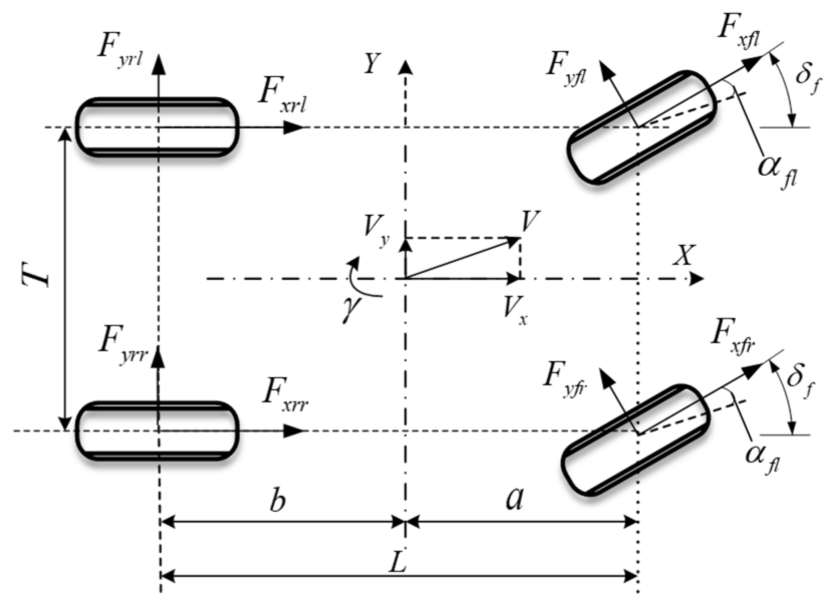
The driving direction in front of the vehicle is taken as the longitudinal coordinate X axis, and the left direction when the vehicle is driving forward is the lateral coordinate Y axis. When the vehicle turns to the left, according to D’Alembert’s theorem, the differential equations for the longitudinal, lateral, and yaw motion of the vehicle system are established [37], as shown in Figure 1.
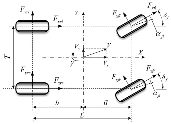
Figure 1.
The vehicle dynamics model.
The differential equation of motion is established as follows [37,38]:
Longitudinal motion equation:
Lateral motion equation:
Yaw motion equation:
where is the mass of the whole vehicle, is the yaw angular velocity, is the front wheel angle, and are the longitudinal and lateral acceleration, respectively. are the longitudinal and lateral velocities of the vehicle center of mass, respectively, are the front and rear wheel tracks, and are the longitudinal and lateral force of each tire. are the left front wheel, right front wheel, left rear wheel, and right rear wheel, respectively, and is the moment of inertia of the whole vehicle around the z-axis. is the yawing moment.
As pavement information mostly appears in adhesion coefficient form, the influence of roughness is often ignored. To provide an accurate representation of the contact between the tire and the three-dimensional pavement while driving, as referenced in [25], the stress distribution and multi-point contact model were utilized in the vertical dynamics model. This discretizes the surface contact between tire and pavement into a multi-point contact and gives different weight coefficients to each point based on the law of stress distribution.
The vertical load of a vehicle under a three-dimensional road can be expressed as follows [25]:
where m and n are the number of contact points between the edge area and the central area. , and are the tire distribution damping coefficient, tire stiffness coefficient, and suspension stiffness coefficient, respectively. , and are the tire distribution damping coefficient, suspension damping coefficient, and tire damping coefficient, respectively. g is 9.8 m/s2. is the vertical displacement of the car body. is the roll angle of the car body, is the height of the center of mass, is Wheelbase, is total vehicle mass, is sprung mass. are the distance from the center of mass to the front and rear axes. represents the discretized road roughness. The average contact stress ratio between the central and edge regions of a radial tire is approximately 1.2, which is used as the weighting coefficient for the contact area [25].
3. Estimation Strategy Based on a Dimensionless Tire Model
3.1. Construction of the Dimensionless Tire Model Based on Standardized Processing
This paper proposes a novel dimensionless tire model. The coefficient of adhesion and the peak adhesion coefficient between adjacent pavements in the Burckhard curve are now correlated in this model. This correlation has enabled the establishment of a direct mapping relationship between the peak adhesion coefficient of a target pavement and the typical mechanical tire characteristics under such pavements.
3.1.1. Burckhardt Model
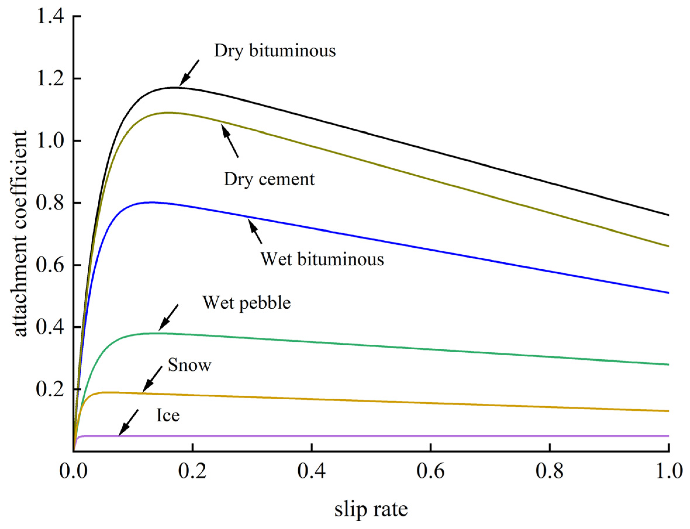
Burckhardt and colleagues fitted the curves of six typical pavements (by using the adhesion coefficient slip rate through numerous experiments [39] and constructed a practical tire–pavement mathematical model that is widely used in automobile dynamics research. Its expression is as follows:
where , , and are the parameter values of each typical pavement, as shown in Table 1. The parameters are derived from reference [25].

Table 1.
Parameter values of each typical pavement.
According to Formula (10) and the parameter values in Table 1, the curves of six common pavements can be seen in Figure 2.
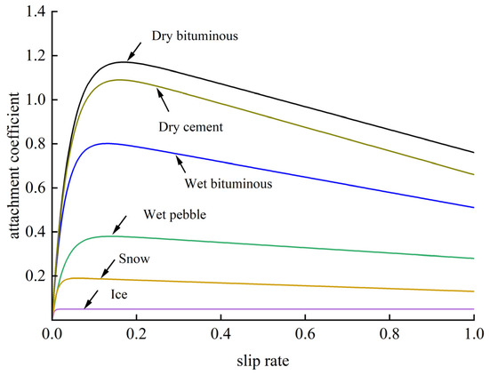
Figure 2.
Typical road adhesion coefficient curves.
As can be seen in Figure 2, the curves of six typical pavements are particularly similar, and the trend of their nonlinear changes has the following two laws:
- (1)
- As the slip rate goes up, the adhesion coefficient initially increases but then decreases over time.
- (2)
- Within the small initial range of the slip rate [0, 0.05], there is little difference in the adhesion coefficients of six typical pavements. However, in the range of the subsequent slip rate [0.05, 1], the adhesion coefficient of each pavement is different.
Therefore, the curves corresponding to different pavements are different, which is the inherent characteristic of each pavement. Furthermore, the points on each pavement curve can represent the adhesion characteristics of the pavement, which can be used as an essential basis for pavement identification.
3.1.2. A Dimensionless Tire Model Based on Standardized Processing
As illustrated in Figure 3, when the utilization coefficient of the friction point of an unknown road surface lies within the curves of two typical road surface adhesion coefficients, it can be determined that the peak adhesion coefficient of this road surface also falls between the peak adhesion coefficients of the two adjacent surfaces.
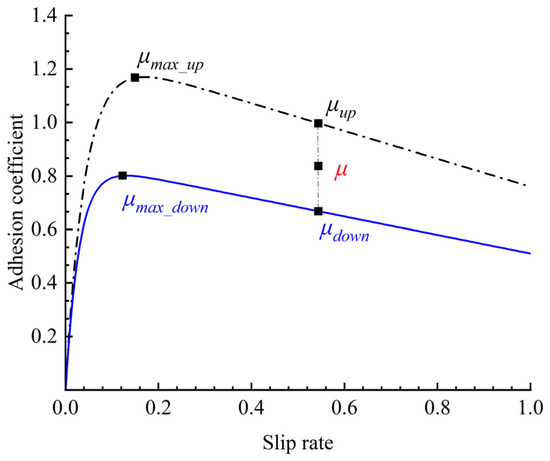
Figure 3.
Identification algorithm diagram.
As shown in Figure 3, in order to accurately predict the peak adhesion coefficient between typical pavements, it is considered that the target pavement has a certain commonness with two similar pavements. When considering the difference between the adhesion coefficient of the typical pavements and the peak adhesion coefficient, it can be considered that the peak adhesion coefficient law between the target pavement and the typical pavement to be identified is as follows [24]:
where , , and are the peak adhesion coefficients of the pavement to be identified and the two adjacent pavements, respectively. , , and are the utilization adhesion coefficients of the pavement to be identified and the two adjacent pavements, respectively.
Formula (12) can be derived as follows:
To verify the prediction accuracy of the pavement adhesion coefficient algorithm proposed in this paper, three pavements adjacent to the typical pavement were first selected. Then, the pavement with the highest adhesion coefficient and the pavement with the lowest adhesion coefficient among the three were used as reference pavements for the prediction algorithm, thereby predicting the pavement with a medium adhesion coefficient.
The prediction deviation and the average prediction deviation were selected as the accuracy indexes of the evaluation results, and the formula for this is shown in Formula (14):
where is estimated by the algorithm using the adhesion coefficient.
Based on the above methods, dry cement pavement, wet bituminous pavement, wet cobblestone pavement, and snow-covered pavement were identified. The calculated identification results are shown in Figure 4.
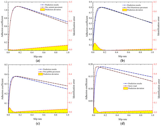
Figure 4.
Road identification results: (a) Dry cement prediction results. (b) Wet bituminous prediction results. (c) Wet pebble prediction results. (d) Snow road prediction results.
As can be observed in Figure 4, the prediction deviation of the typical pavement was 2~8%, and the average prediction deviation was 1.97%, 0.88%, 1.76%, and 1.26%, respectively.
To summarize, the pavement prediction algorithm is capable of accurately predicting the adhesion coefficient of the present pavement. It also provides a theoretical basis for the subsequent algorithm.
The longitudinal slip rate can be expressed as follows [40]:
where is the wheel angular velocity, is the tire rolling radius, and is the longitudinal speed of the tire center.
The lateral slip rate can be expressed as follows [40]:
where is the tire slip angle.
The comprehensive slip rate can be expressed as follows [16]:
By combining Equations (13), (16) and (17), the adhesion coefficient of longitudinal and lateral utilization pavement can be expressed as the following:
The comprehensive friction of tires can be expressed as follows [16]:
By combining Equations (12) and (19), the following can be deduced:
where , , are the tire forces of the pavement to be identified and the adjacent typical pavement, respectively.
To summarize, when combined with Formulas (19)–(21), the longitudinal and lateral force of the tire can be expressed as follows:
where is the tire force after the dimensionless parameter, which has nothing to do with the road surface to be identified. , , , and are the lateral and longitudinal force of the tire under the typical pavement. As the parameters of typical pavement are known, the database of mechanical tire characteristics under typical pavements can be established in advance. The magic formula tire model is obtained by fitting many tire test data. Due to its high accuracy and versatility, it is extensively utilized for vehicle dynamics simulations and analysis in various applications. Therefore, the data for the mechanical tire characteristics of a typical pavement in this paper were obtained by fitting the magic tire in reference [16], such that the tire force of the typical pavement, , , and the adhesion coefficient of the pavement to be identified can be used to indicate the force on the tire of the pavement to be identified.
3.1.3. Verification of the Dimensionless Tire Model
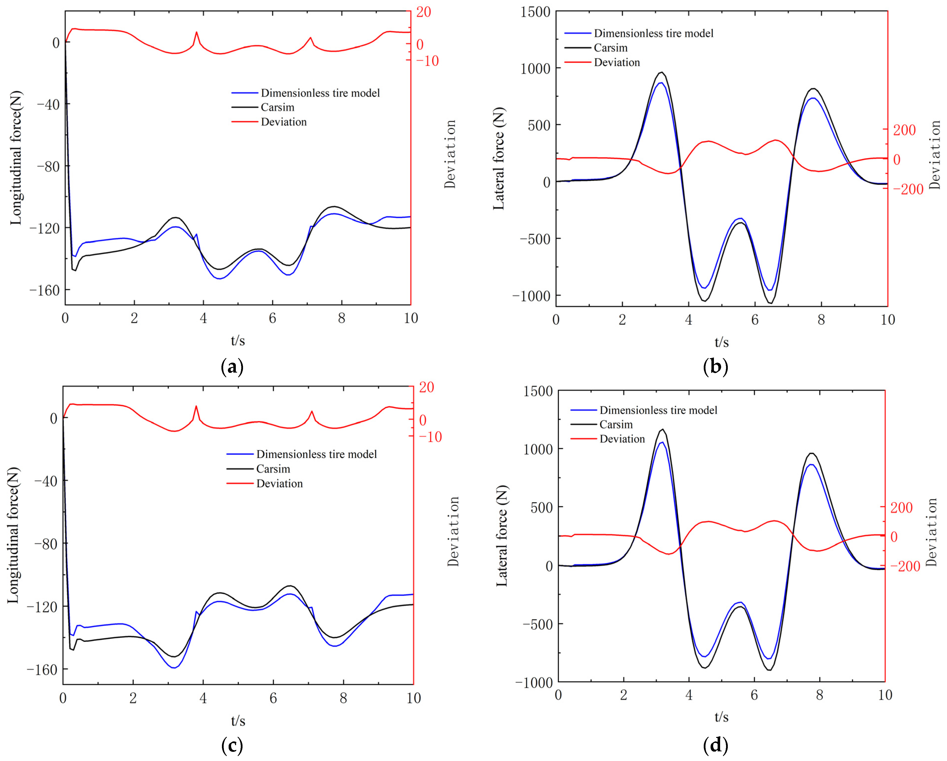
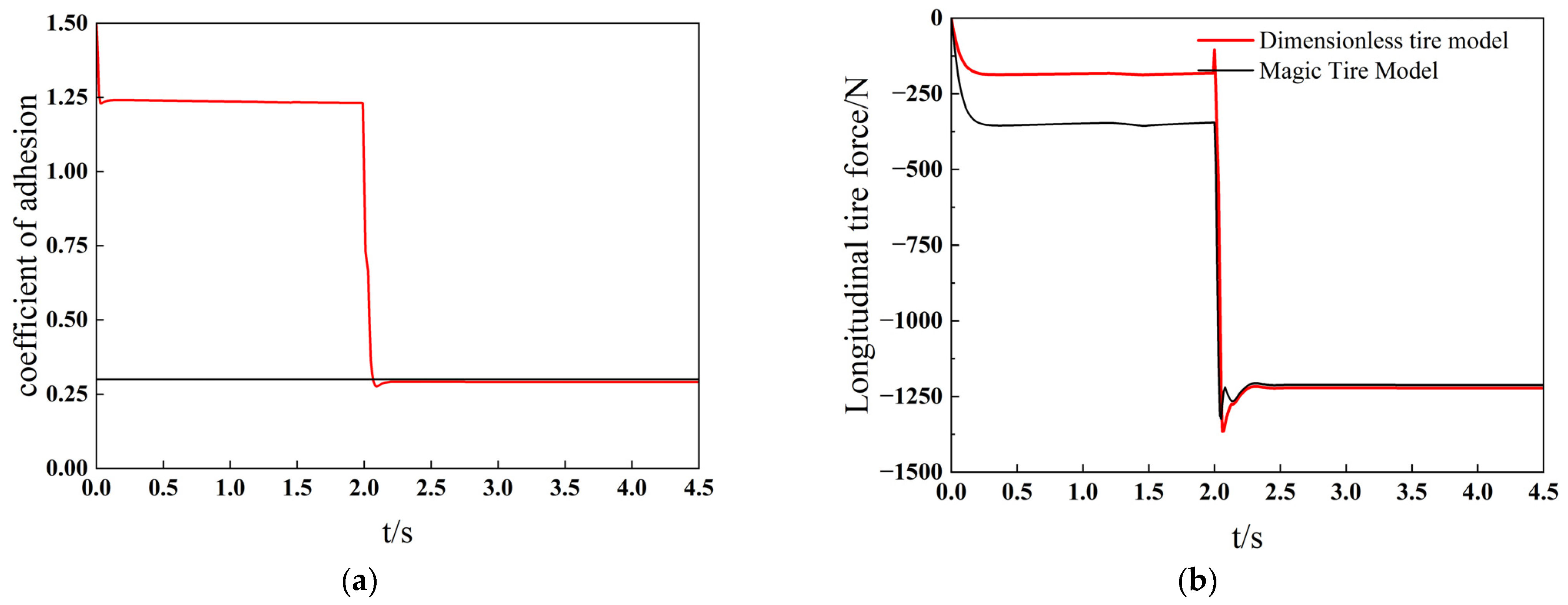
To validate the dimensionless tire model, this paper selected a dual-lane change scenario for testing. Figure 5 confirms the longitudinal and lateral forces of the tire under simulation conditions, with the vehicle initially traveling at 80 km/h and maintaining a steady speed, not exceeding a maximum limit of 90 km/h. The road surface was simulated as a typical bituminous road, and the forces of two different tire models were compared under mixed condition scenarios.
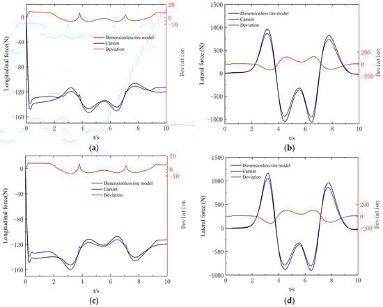
Figure 5.
Tire force comparison results: (a) Longitudinal force of left front wheel (b) Left front wheel lateral force. (c) Longitudinal force of right front wheel. (d) Right front wheel lateral force.
By comparing the data of the two kinds of tires with the relative root mean square deviation and the relative root mean square deviation, we obtain Formula (26):
where is the simulation data and is the experimental data.
The RRMSE value of the longitudinal force of the left front wheel was less than 0.0412, the RRMSE value of the lateral force was less than 0.0033, the RRMSE value of the longitudinal force of the right front wheel was less than 0.0417, and the RRMSE value of the lateral force was less than 0.0036. The overall estimation deviation is less than 7%. The comparative data show that the standardized tire model can accurately represent the longitudinal mechanical characteristics and lateral mechanical characteristics of the interactions between the tire and road surfaces during vehicle driving, and it also has good adaptability.
In the tire model, the tire force from a typical road surface is sufficient to achieve characteristics that closely approximate those of the Magic Tire model. This parameter has good adaptability and predictability for complex and changeable road conditions and is of great importance in the active control of vehicle safety.
This tire model simplifies the complex mechanical interactions between the tire and the road in order to improve computational efficiency and real-time simulation capabilities. However, these simplifications often overlook some of the complex factors in the tire-road interaction, such as tire deformation, slip distribution across the contact patch, and road surface variations. As a result, under extreme conditions, such as high slip ratios, heavy loads, or extreme cornering, the simplified model may not fully capture the true tire behavior, leading to inaccuracies in predictions.
3.2. Estimation of the Peak Adhesion Coefficient Based on UKF
The common method for estimation is the Kalman filter algorithm, which has been applied in many pieces of literature at home and abroad [24]. Moreover, it has achieved specific results in parameter estimations. The Kalman filter algorithm is based on a square minimum mean square error autoregressive data processing method. At the same time, the unscented Kalman filter (UKF) is used to approximate the probability distribution of nonlinear systems, and the theoretical and practical results show that its accuracy is higher than that of the standard Kalman filter. Therefore, this paper uses the unscented Kalman filter (UKF) to estimate the adhesion coefficient.
3.2.1. Establishing the System Equation of the Estimation Algorithm
According to Equations (28), (29) and (37), the state equation and measurement equation of the system can be obtained. Among them, the state equation can be expressed as follows:
The measurement equation can be expressed as
where is the peak adhesion coefficient between the four tires and the road surface and the sum of random variables and , which are process noise and measurement noise, respectively. The H(x, y) in Equations (36) and (37) is a supplement to Equation (35).
3.2.2. UKF Estimation Algorithm
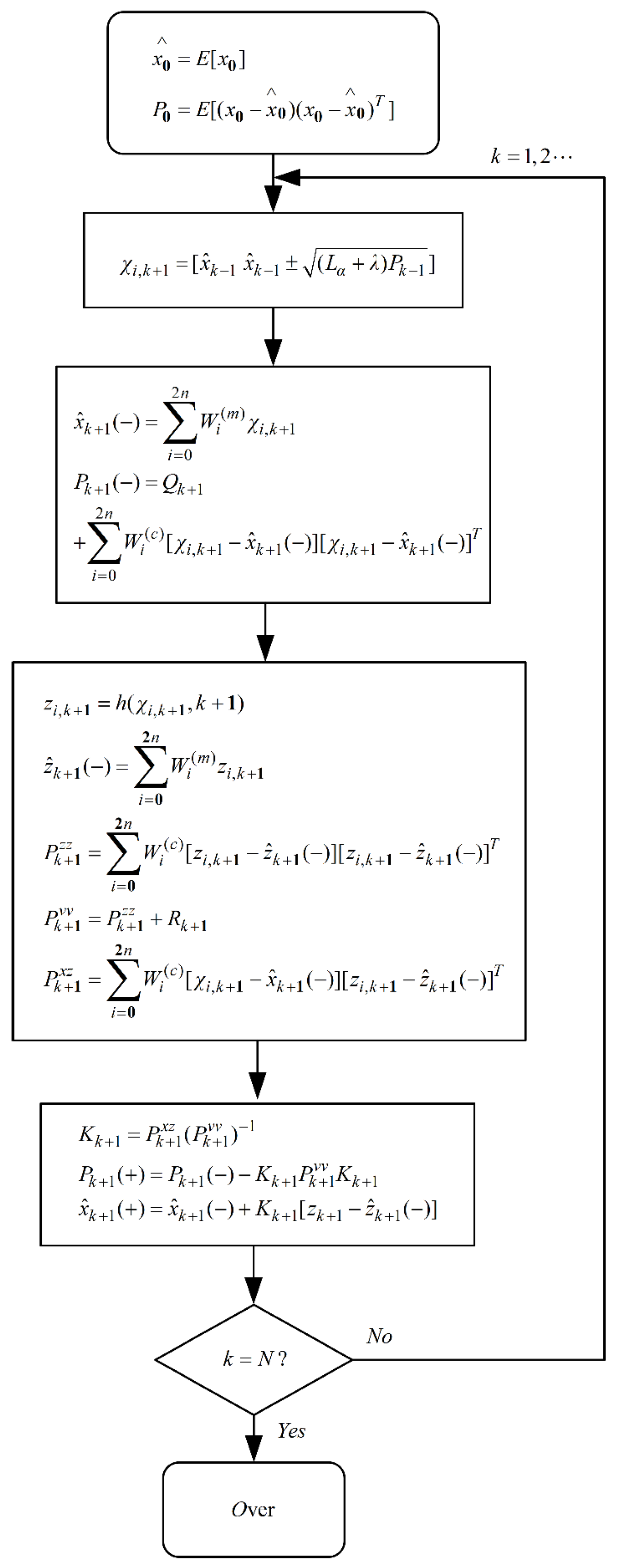
The estimation flow for the extended Kalman filter algorithm is shown in Figure 6.
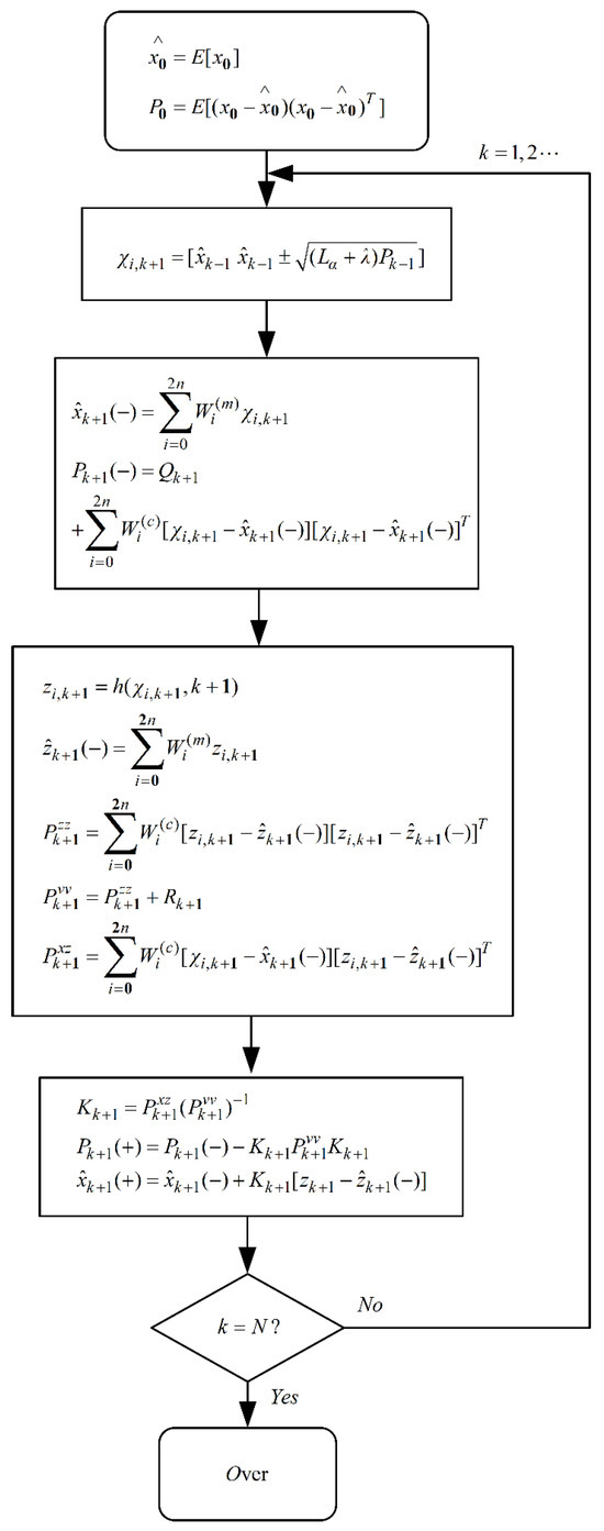
Figure 6.
UKF process chart.
The measurement noise covariance is , the covariance of process noise is , the initial error covariance is , and the initial state matrix is .
3.2.3. Algorithm Process
Figure 7 is a flowchart of the UKF estimation algorithm, and it is based on the peak adhesion coefficient of the normalized tire model.
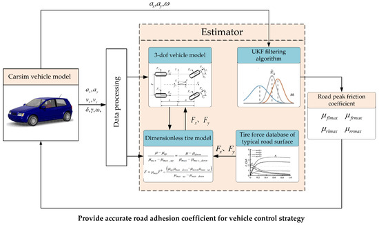
Figure 7.
Road peak adhesion coefficient estimation flow chart.
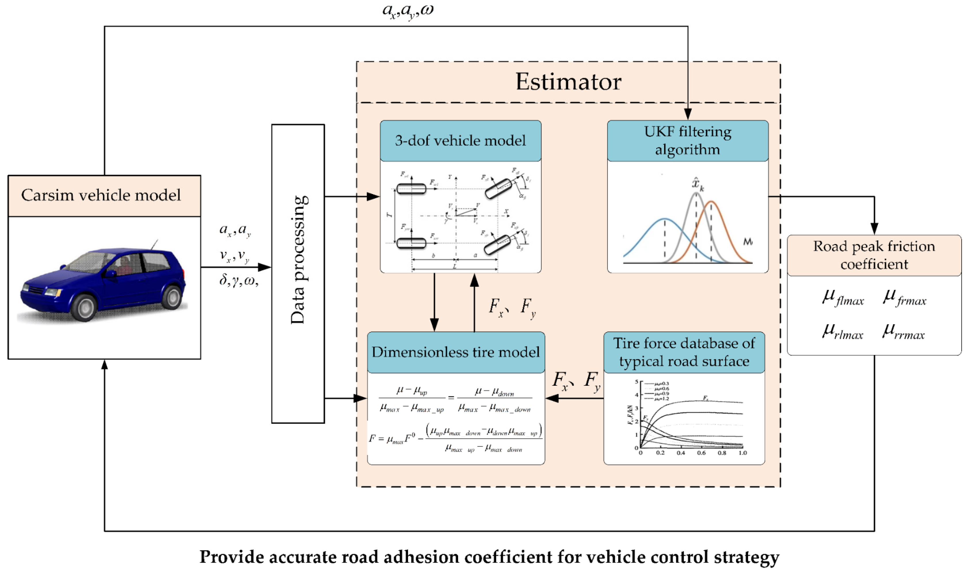
Step 1: Output the experimental parameters (e.g., lateral acceleration, longitudinal acceleration, vehicle angular velocity, tire speed) through the vehicle’s sensors. After signal processing, it is used as the input signal of the subsequent dynamic model and Kalman filter.
Step 2: The vehicle dynamics model includes the plane and vertical dynamics models. After combining the proper vehicle parameters with the dynamics model, we can obtain the experimental parameters needed to standardize the tire. After algorithm processing, we can establish the direct relationship (standardization) between the target road surface’s peak adhesion coefficient and the tire’s mechanical characteristics under the typical road surface.
Step 3: Combine the normalized tire force with the dynamic model and transform it into the form of the state space equation required by UKF.
Step 4: Complete the estimation of the maximum adhesion coefficient through UKF.
Step 5: Transfer the estimated adhesion coefficient to the running vehicle, which provides a basis for the active safety control algorithm.
The results of this algorithm’s estimation can be found in Section 5.
4. Estimation Algorithm Based on Adaptive Variable Domain Fuzzy Strategy (AVUFS)
The utilization adhesion coefficient of pavement is a typical follow-up system. As the utilization adhesion coefficient will constantly change with the driving state of the vehicle and the working conditions of the pavement, and as the vehicle itself has a severe nonlinear relationship, the prediction algorithm needs to have an excellent dynamic response speed and adaptive ability to the nonlinearity parameter in order to deliver the estimation of the peak adhesion coefficient. The fuzzy logic algorithm imitates the fuzzy thinking process of the human brain by establishing fuzzy sets. This algorithm is considered an effective method for solving the problem of nonlinear system model estimations and predictions, and it is widely used in engineering systems [41,42].
However, the estimated effect of the fuzzy algorithm with a single and fixed structure mainly depends on membership function, rule base, and fuzzy reasoning, which leads to the problems of contingency, low prediction accuracy, and the intense subjectivity of fuzzy algorithms. Therefore, to achieve the best control effect, optimizing the design of the fuzzy algorithm is necessary.
Therefore, this paper proposes a variable universe fuzzy algorithm, which improves the traditional fixed membership function into a time-varying membership function. This algorithm can constantly update and optimize the membership function according to the driving state of the vehicle. The utilization of particle swarm optimization is introduced in this paper to significantly improve the design of the membership function and ensure that it is always in the best estimation range, thus improving the adaptability and estimation accuracy of the fuzzy algorithm. Moreover, the optimization process only improves the algorithm, which is convenient in design and fast in operation; however, it can effectively improve the shortcomings of single fuzzy control and has a high application value.
4.1. Pavement Characteristic Factor
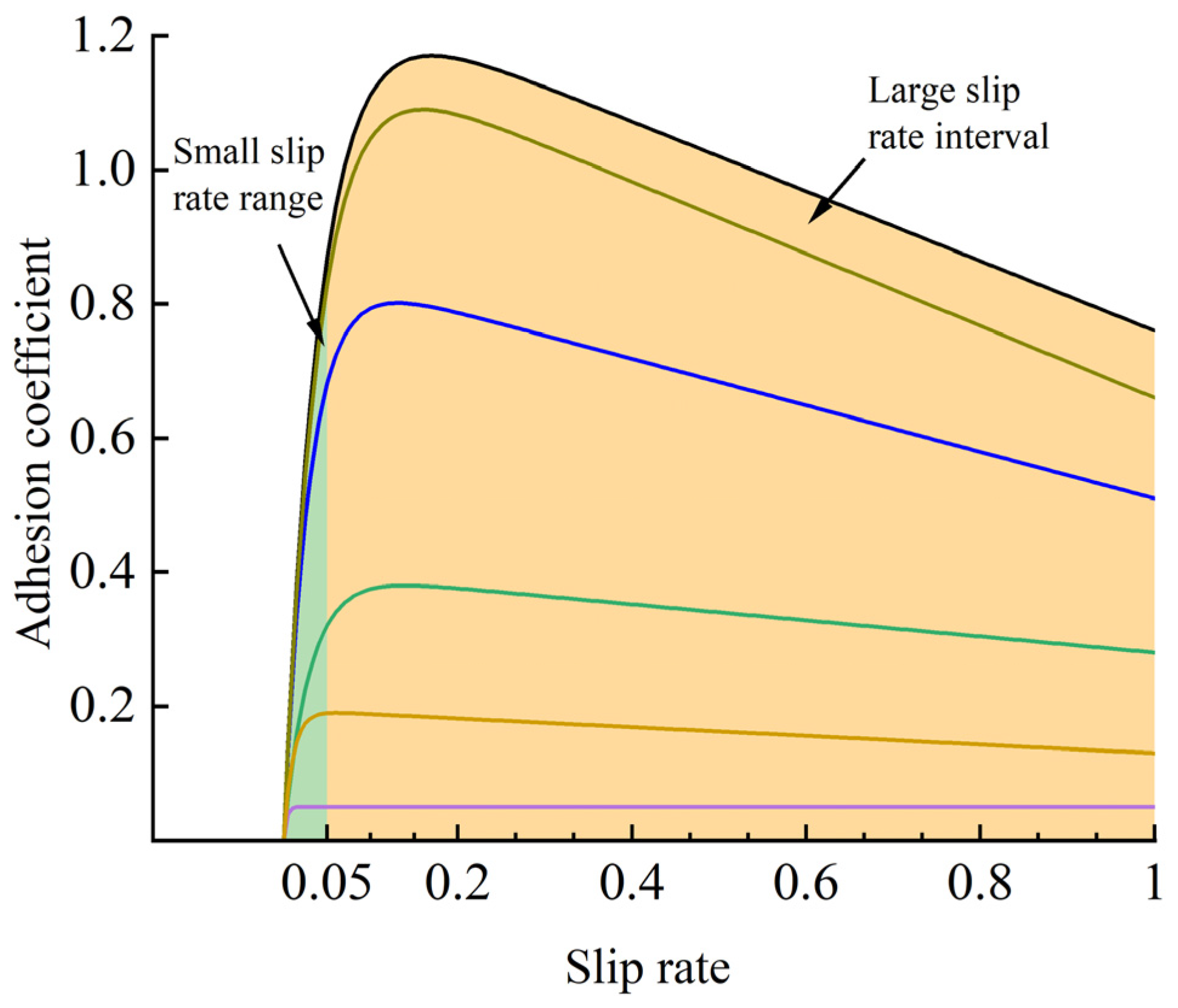
Based on the curve of the typical pavements in the Burckhard tire model, it can be found that the slip rate of the six typical pavements is especially low in the initial [0, 0.05] area; however, in the slip rate range of [0.05, 1], the adhesion coefficient of the pavement is evidently different. Therefore, according to the characteristics of the adhesion coefficient of the slip rate in different stages, this paper (as shown in Figure 8) divides the slip rate into two sections: small slip rate and large slip rate.
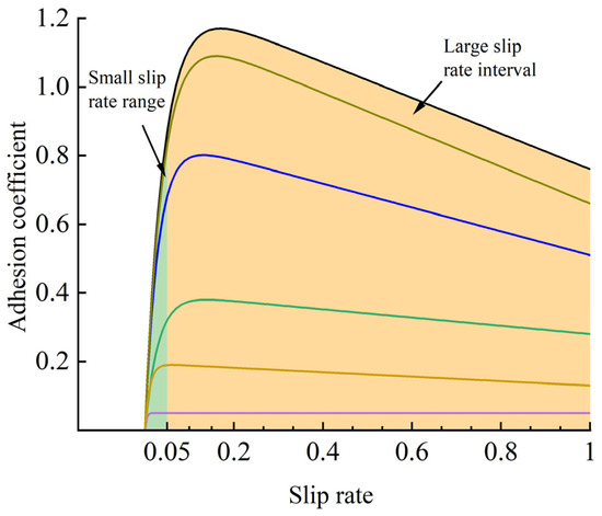
Figure 8.
Interval division diagram.
In this section, we employed the derivative method to characterize the variation in the pavement adhesion coefficient. The primary advantage of this method lies in its ability to accurately capture the dynamic changes in the adhesion coefficient at different slip ratios, particularly under low slip ratios, where it can still effectively identify pavement features and estimate pavement types. This method not only provides a more comprehensive description of the friction characteristics of pavements under various conditions but also allows for real-time reflection of how different pavement features affect adhesion performance. Based on relevant literature [43,44,45], the derivative method, compared to traditional static methods, offers higher flexibility and demonstrates better adaptability and accuracy in variable real-world road conditions, especially at low slip ratios, where it can effectively capture subtle changes in the pavement.
When the slip ratio is [0, 0.05], there is little difference in the adhesion coefficient of the pavement. In this paper, the concept of the Pavement Characteristic Factor is put forward and used as the parameter index for pavement predictions. Its definition is as follows:
where is the pavement characteristic coefficient, is the slip rate, is the pavement adhesion coefficient, and is the slope of the adhesion coefficient curve.
By differentiating Formula (1), the following can be obtained:
The derivations from Formulas (34) and (35) can be obtained as follows:
By combining the pavement mentioned above’s characteristic factor expression (36) and the parameter values in Table 1, we can obtain the varying characteristic adhesion curves of six typical pavements with the slip rate, as shown in Figure 9.
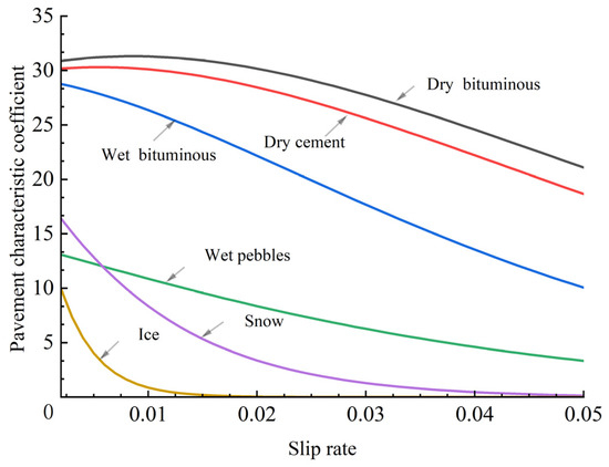
Figure 9.
The characteristic curves of the typical pavements.
As can be seen from Figure 10, when the slip ratio is [0, 0.05], the pavement characteristic coefficients are clearly distinguished. Although there are a few intersections between the six typical pavements, it does not affect the classification and extraction of the pavement characteristic values. The adhesion coefficient of each pavement varies when the slip rate falls within the range of 0.05 to 1; thus, the curves of the typical pavements are directly used for extraction.
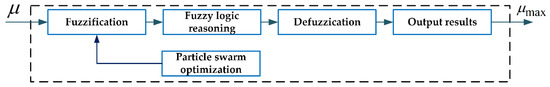
Figure 10.
Fuzzy logic observer.
By introducing the Pavement Characteristic Factor method, even when the slip rate is less than 0.05, the adhesion features of typical pavements can still be clearly distinguished and extracted, providing a basis for the subsequent variable universe fuzzy algorithm.
While the algorithm has been theoretically validated for feasibility and effectiveness, it has only been tested in an idealized environment. This testing setup oversimplifies the real-world challenges, such as noise interference that might be encountered in actual settings, and it has not been practically validated with real vehicle tires. This scenario underlines the need for further testing under more realistic conditions to fully ascertain the algorithm’s applicability and robustness.
4.2. Particle Swarm Optimization Algorithm
Particle swarm optimization (PSO) is a numerical calculation method that utilizes an evolutionary algorithm to find the optimal solution through iterative processes [46,47]. The algorithm updates the information of each particle group by considering both the individual optimal value (Pbest) and the group optimal value (Gbest), and it solves the fitness function by using the objective function. By doing so, PSO can efficiently obtain the optimal solution.
In an N-dimensional space with a number of particle groups, the velocity and position of each particle (m) in the group can be expressed: and . Furthermore, the expression of the particle velocity and position update is as follows:
where expresses the inertia weight of the particles, and are different learning factors, and represent the random numbers in the interval [0, 1], and m = 1, 2….a is mainly responsible for constraining the velocity and rebound of the boundary particles.
4.3. Adaptive Variable Universe Fuzzy Strategy (AVUFS)
This paper uses a fuzzy logic algorithm to estimate the nonlinear mapping relationship between the adherence coefficient and the peak adherence coefficient. The fuzzy logic model is a system that takes in one input and produces one output. In other words, it uses the real-time utilization adhesion coefficient of the tire as the input and calculates the peak adhesion coefficient of the pavement as the output. Figure 10 shows the structure of a fuzzy logic observer.
It consists of the following four steps:
- (1)
- Fuzzification
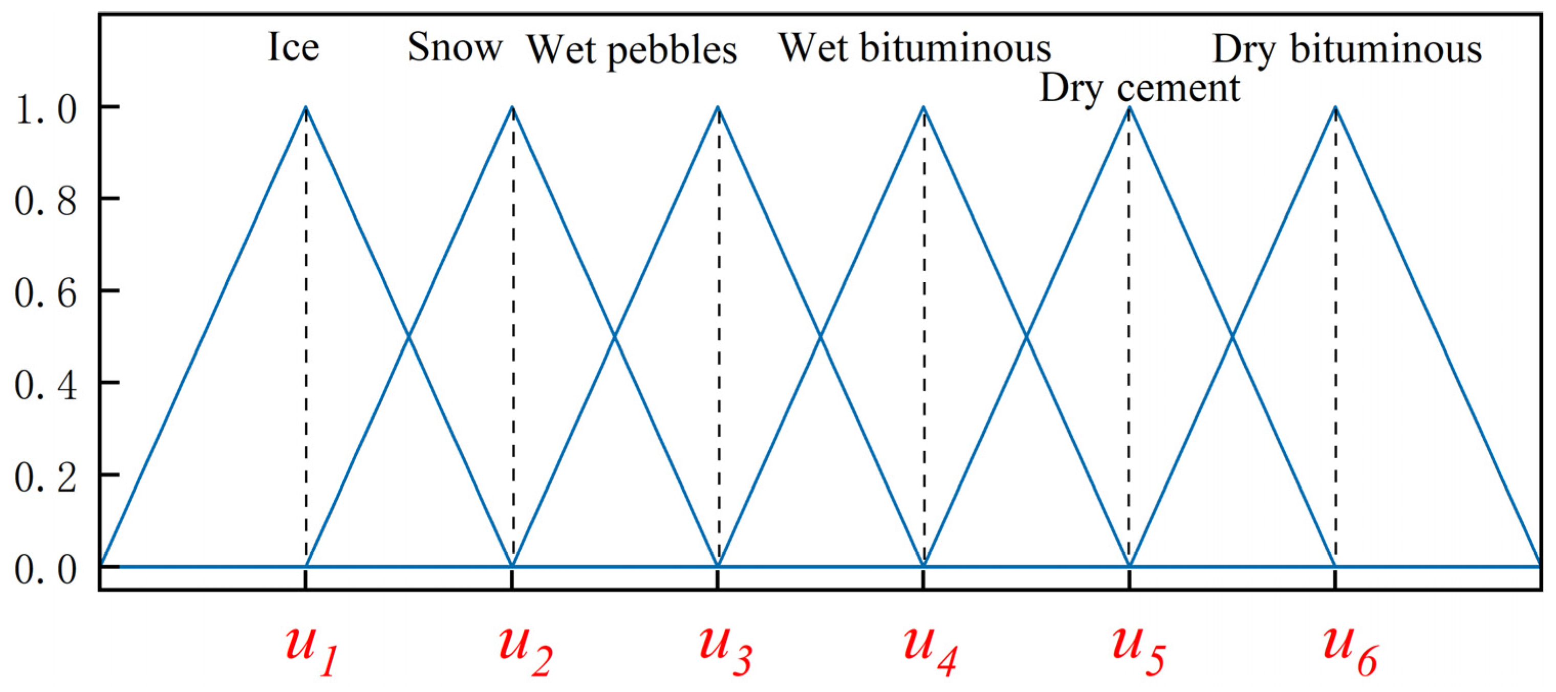
To make the utilization adhesion coefficient more understandable, we established six fuzzy subsets that cover the entire fuzzy universe. This approach helps to fuzzify the apparent value of the utilization adhesion coefficient. The fuzzy sets can be defined as follows:
{μ} = {Ice, snow, wet pebbles, wet bituminous, dry cement, and dry bituminous}
The membership function is selected as a trigonometric function, as shown in Figure 11.
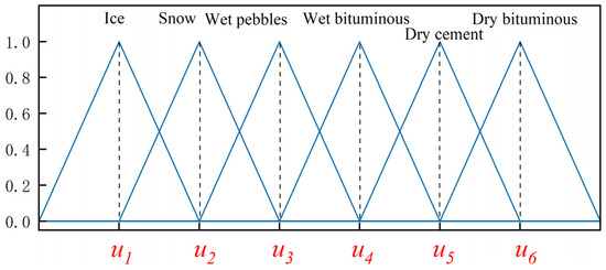
Figure 11.
Membership function diagram.
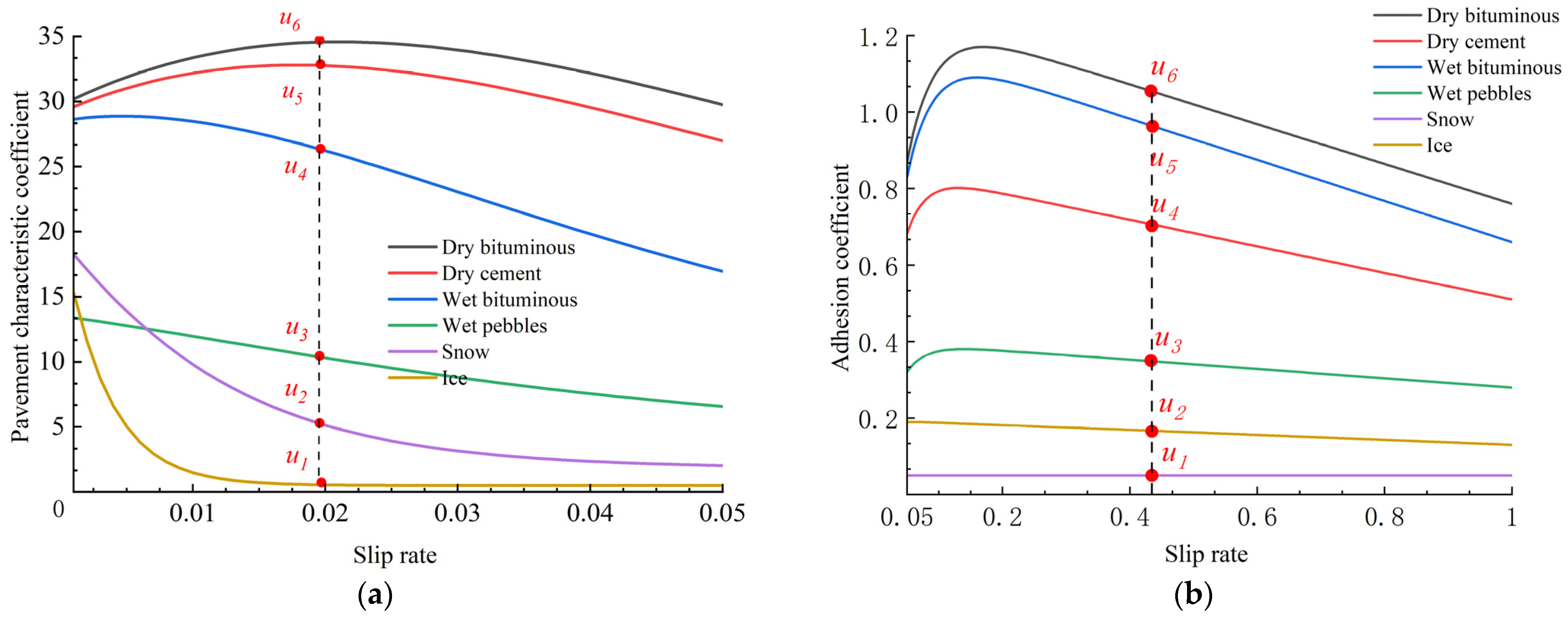
The utilization of the adhesion coefficient between the tire and road surface constantly changes due to the varying driving states of the vehicle and road conditions. To ensure accurate estimation, it is essential to create an adaptive membership function that adjusts to these nonlinear changes. For this reason, this paper adopts the method of subsection prediction. At the stage of small slip rates, the adhesion characteristics u1, u2, u3, u4, u5, and u6 of the pavement are extracted by using the pavement feature factors, as shown in Figure 12a. In the stages of significant slip rate, the Burckhardt model is used to directly extract the adhesion coefficients u1, u2, u3, u4, u5, and u6, as shown in Figure 12b.
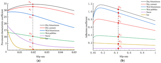
Figure 12.
The utilization adhesion coefficient membership function: (a) Small slip-rate-adhesion characteristics. (b) Large slip-rate-adhesion coefficient.
As the slip rate constantly changes during the vehicle’s operation, the extracted adhesion characteristic values—u1, u2, u3, u4, u5, and u6—of each typical road surface are also always changing, thus establishing the following membership function.
Given the peak adhesion coefficient of a typical pavement, six fuzzy subsets spanning the entire fuzzy universe are defined to specify the peak adhesion coefficient. The fuzzy sets can be defined as follows:
{μmax} = {Ice, snow, wet pebbles, wet bituminous, dry cement, dry bituminous}
- (2)
- Fuzzy decision process
Fuzzy reasoning is the core part of the whole method, and it plays a vital role in the output results. Fuzzy reasoning rules are formulated based on the relationship between the adhesion coefficients of typical pavements and the peak adhesion coefficient. The fuzzy rules are shown in Table 2.
Table 2.
Fuzzy inference rule table.
- (3)
- Defuzzification
The output obtained by fuzzification and fuzzy logic reasoning needs to be clarified to obtain the required output. Based on the peak adhesion coefficient of the six typical pavements, the membership function of the output is formulated. As shown in Figure 13, the centroid method is used to convert the fuzzy value into a precise value for deblurring.
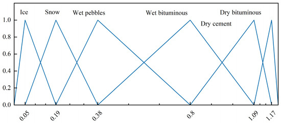
Figure 13.
Peak adhesion coefficient membership function diagram.
- (4)
- Optimized membership function
Based on particle swarm optimization, the membership function of the typical pavements is optimized through the existing experimental data, and it mainly optimizes the boundary values an and bn of each membership function, as shown in Figure 14.
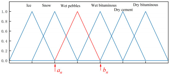
Figure 14.
Adhesion coefficient membership function.
Particle swarm optimization is mainly divided into four steps:
- (1)
- Initialize the number, position, and speed of boundary values and .
- (2)
- Thus, the fitness function of boundary values and the optimal values of individuals and groups are obtained.
- (3)
- Update the position and velocity of each boundary value and from Equations (7) and (8).
- (4)
- Obtain the fitness function, as well as the individual and group optimal values of the boundary values an and bn. If the calculated value is not the optimal solution, return to Step (3) to update the particles until the optimal solution is found.
Through the optimization of particle swarm optimization, the boundary values and of the optimal membership function are continuously searched.
4.4. Estimation Process
Figure 15 is a flowchart of the variable universe fuzzy adhesion coefficient estimation algorithm.
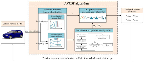
Figure 15.
Estimation of the Fuzzy Adhesion Coefficient in the Variable Universe for Particle Swarm Optimization.
Step 1: The real-time slip rate between the tire and the road is measured by a dynamic model and sensor.
Step 2: The dynamic adhesion coefficient is extracted between the regions according to the slip rate.
Step 3: Take the time-varying adhesion coefficient as the input of the adaptive variable universe fuzzy algorithm and calculate the peak adhesion coefficient of the pavement.
Step 4: Transfer the estimated adhesion coefficient to the running vehicle, which provides a basis for the active safety control algorithm.
4.5. Simulation Verification of the Pavement Identification Algorithm
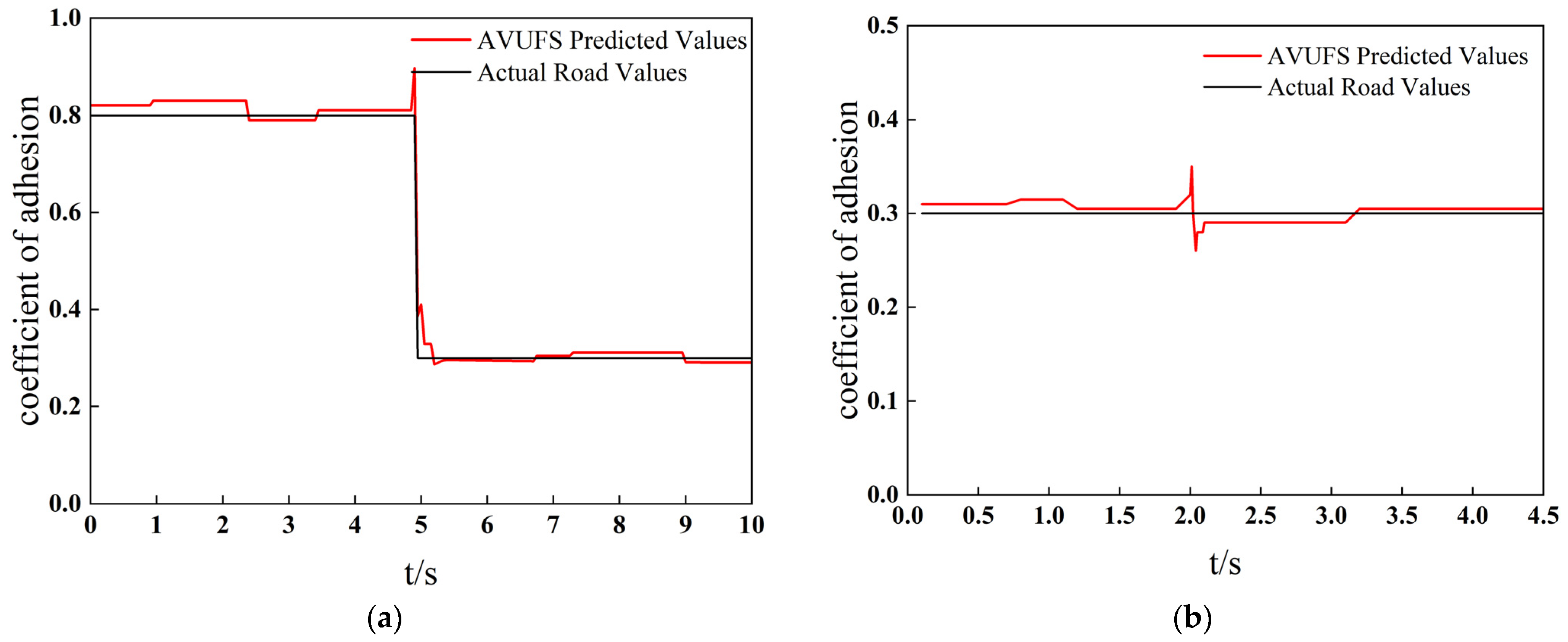
As a check on the accuracy of the algorithm, the adhesion coefficient of use of the six typical pavements in Burckhardt’s tire model was used as the input value for the fuzzy algorithm, and the results of this can be seen in Figure 16.
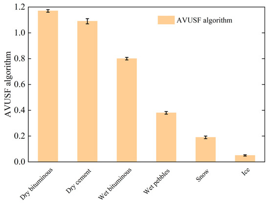
Figure 16.
Identification results of the AVUSF algorithm.
As shown in Figure 16, the prediction results for the six typical road surfaces have a maximum deviation of no more than 1%, indicating high accuracy. This demonstrates that the algorithm can accurately predict the peak adhesion coefficients of typical road surfaces.
5. The Verification and Fusion Strategy of Joint Simulation
In this simulation experiment, an E-class vehicle was selected as the experimental vehicle, using a four-wheel independent drive powertrain, and the dimensionless tire model proposed in this paper was employed. To simplify the calculation, the effect of air resistance was ignored, and the aerodynamic module was disabled in the simulation software. The basic parameters of the vehicle model are shown in Table 3, with the gravitational acceleration g = 9.8 m/s2.
Table 3.
Key parameters of the vehicle.
5.1. Estimation Results Based on Dimensionless Tires
In the simulation software, gear control was set to neutral, with no steering control. The longitudinal control used an open-loop throttle control, with the initial vehicle speed set to 120 km/h and the throttle opening to 0. The brake wheel cylinder pressure was set to 0 for the first 2 s and then gradually increased from 0 to 4 MPa, remaining constant at 4 MPa thereafter. The constructed road model in the simulation is as follows: the 0–130 m section simulates an asphalt road with an adhesion coefficient of 0.8, and the section from 130 m onward simulates an icy or snowy road with an adhesion coefficient of 0.3.
Figure 17 shows the estimated results of the adhesion coefficient. From Figure 17a, it can be seen that during the first 2 s, the vehicle travels at a constant speed, and the adhesion coefficient is not effectively estimated. During this period, Figure 17b indicates that the vehicle’s slip ratio remains below 5%, preventing the dynamic friction characteristics between the tire and the road from being fully activated. This makes it difficult for the tire model to accurately represent the complex friction relationship between the tire and the road. At the same time, the longitudinal acceleration xa is close to 0, and the residual term is also 0, leading to the inability to effectively correct the prior estimate, resulting in an inaccurate posterior estimate.
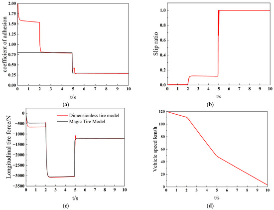
Figure 17.
Simulation results under high-speed conditions. (a) Adhesion Coefficient Estimation Results. (b) Slip Ratio Results. (c) Comparison Results of Tire Longitudinal Force. (d) Vehicle Speed.
At the 2-s mark, the braking force gradually increases, and the UKF algorithm’s estimated value gradually rises within 0.2 s, approaching the true value and stabilizing around 0.81. Around the 5-s mark (130 m), the adhesion coefficient drops from 0.8 to 0.4, and the estimated result exhibits a brief fluctuation. This is due to a transient change in the tire forces, causing the dimensionless tire model to fail to follow the changes rapidly, resulting in a large instantaneous error, as shown in Figure 17c. After approximately 0.2 s of brief fluctuations, the tire model’s estimated value stabilizes and continues to follow the true value, settling around 0.29. The error in the stable phase is less than 0.01.
To validate the accuracy of the estimation algorithm at low speeds, the following simulation settings were used: longitudinal control was set at an initial speed of 30 km/h with open-loop throttle control, throttle opening was 0, brake cylinder pressure was 0 for the first 2 s, and then gradually increased to 4 MPa and maintained. The road surface’s adhesion coefficient was set at 0.3, simulating icy and snowy conditions.
Simulation results, as shown in Figure 18, include the estimated results of the adhesion coefficient (Figure 18a) and longitudinal force (Figure 18b) of the right front wheel. As seen in Figure 18a, similar to the high-speed condition, the adhesion coefficient could not be effectively estimated during the first 2 s of uniform driving. When the braking force began to increase at the 2-s mark, the UKF algorithm’s estimated value quickly adjusted to near the true value within 0.2 s, stabilizing at about 0.29, with an error of less than 0.01 during the stable phase.
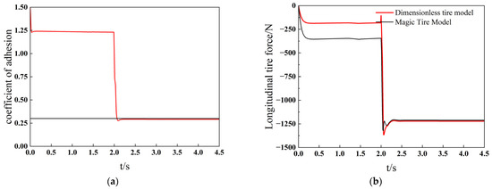
Figure 18.
Simulation Results Under Low-Speed Conditions. (a) Adhesion Coefficient Estimation Results. (b) Comparison Results of Tire Longitudinal Force.
The algorithm exhibits the following characteristics:
Advantages:
At high slip ratios, the estimation results are relatively stable, effectively reflecting the peak adhesion characteristics of the road surface.
The general trend and magnitude of the tire’s longitudinal force are consistent with actual results, validating the accuracy of the tire model.
Disadvantages:
There is a larger estimation error at low slip ratios.
The estimation of the adhesion coefficient fluctuates significantly at the initial stage, mainly because the UKF algorithm initially relies heavily on the preset initial information.
When there is a sudden change in the road surface adhesion coefficient, the recognition result exhibits temporary and significant fluctuations.
In summary, although the algorithm performs excellently under specific conditions, further optimization is needed to improve its robustness and accuracy when dealing with low slip ratios and rapidly changing conditions. These results indicate that further research should focus on improving the algorithm’s dependency on initial settings and its dynamic response capability to handle more complex real-road conditions.
5.2. Estimation Results Based on AVUFS
In this algorithm, an adaptive variable universe fuzzy algorithm is established by using the follow-up of the adhesion coefficient between the tire and road, and it is optimized by particle swarm optimization. The estimated adhesion coefficient is shown in Figure 19.

Figure 19.
Adhesion Coefficient Estimation Results With AVUFS: (a) Estimation Results for High-Speed Conditions. (b) Estimation Results for Low-Speed Conditions.
Advantages:
The estimation results of this algorithm are stable in the initial stage and are not affected by the initial conditions.
Although the estimation results fluctuate, the peak adhesion coefficient of the pavement can still be estimated, and its RRMES (Root Relative Mean Squared Error) is 0.0765 and 0.0895, respectively. Even in the small slip rate stage, the peak adhesion coefficient can still be estimated relatively accurately.
When the adhesion coefficient of the pavement suddenly changes, the result can still be estimated quickly and accurately without significant fluctuations.
Disadvantages:
There will be small fluctuations in the estimation process.
5.3. Estimation Results Based on Fusion Strategy
Both methods have certain advantages in estimating the peak adhesion coefficient, but both also have certain limitations; thus, it is necessary to design an integration of the advantages of the two methods.
This paper designs a fusion estimator based on the Kalman gain:
where is the fusion result, and are the estimation result of Strategies 1 and 2, respectively, and is the Kalman gain.
In order to optimize the fusion result, it is necessary to minimize the variance of , which can be expressed as follows:
where , , and are the fusion variance, variance of Strategy 1, and variance of Strategy 2, respectively.
The derivation of the result of (40) can be obtained as follows:
The optimal Kalman gain obtained from Formula (41) is as follows:
To increase the accuracy of the estimation results, this paper implemented a segmentation fusion strategy that utilizes different Kalman gain values at different prediction stages. The specific rules are as follows:
- (1)
- The Kalman gain is set to 0.9572 from the start until the stationary stage.
- (2)
- During the stationary phase, the Kalman gain is set to 0.7189.
- (3)
- The Kalman gain is set to 1 when transitioning from the stationary stage to the abrupt stage.
Figure 20 displays the estimated results, indicating consistent stability throughout the initial stage of prediction and the road surface change stage. The overall estimated results show no noticeable fluctuations. The RRMES of the estimated results were 0.0422 and 0.0406, and the estimation error was less than 3%, surpassing the first two methods. This suggests that the strategy utilized is effective in accurately estimating the peak adhesion coefficient of the road surface.
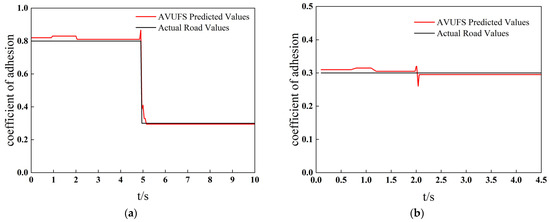
Figure 20.
Adhesion Coefficient Estimation Results with Fusion Strategy: (a) Estimation Results for High-Speed Conditions. (b) Estimation Results for Low-Speed Conditions.
6. Conclusions
To achieve fast and accurate estimation of the peak adhesion coefficient, this paper proposes two algorithms: an adhesion coefficient estimation algorithm based on a dimensionless tire model and an adhesion coefficient estimation algorithm based on an adaptive variable universe fuzzy approach. The advantages of both algorithms are combined, and the estimation results are optimized and fused using the Kalman filter algorithm.
Adhesion Coefficient Estimation Based on the Dimensionless Tire Model: This algorithm establishes a direct mapping relationship between tire mechanical characteristics and peak road adhesion coefficients by analogy with the Burckhardt model. The Unscented Kalman Estimation (UKE) algorithm is used to estimate the adhesion coefficient. Experimental results show that at higher slip ratios, the deviation of the adhesion coefficient is less than 0.05, and the deviation of the tire model is below 7%. The overall estimation is stable; however, the deviation under low slip ratio conditions is relatively large, indicating that further precision improvements are required for low slip ratio conditions.
Adhesion Coefficient Estimation Based on the Adaptive Variable Universe Fuzzy Algorithm: This algorithm improves the traditional fixed-form membership function by introducing a time-varying membership function, which accounts for the dynamic relationship between the tire and road adhesion coefficients. The membership function is continuously updated based on the vehicle’s driving status, ensuring it remains within the optimal estimation range, thus enhancing the algorithm’s adaptability and estimation accuracy. Experimental results show that, for both high and low slip ratio stages, the overall estimation deviation remains stable within 0.02, with minimal dependence on initial values. However, some fluctuations may occur during the prediction process under certain conditions, which requires further research to reduce these inconsistencies.
Fusion Strategy: To further optimize the estimation results, the Kalman filter algorithm is employed to fuse the estimates from both algorithms. Results show that, under complex road conditions, particularly those with alternating low and high adhesion coefficients, the root mean square deviation (RMSD) of the fused algorithm is less than 0.0422, with estimation errors typically below 3%. The estimation results are stable and exhibit high recognition accuracy, although some small fluctuations are still present, indicating that the method can be further optimized. Despite this, the experimental results demonstrate high recognition accuracy and potential for practical control applications. However, further testing and validation in more real-world environments are needed to fully confirm the robustness of the model.
Although simulation results demonstrate that the proposed algorithm achieves promising results in adhesion coefficient estimation, the algorithm still faces several challenges. First, the algorithm has been tested only on passenger vehicles and has not been validated for other types of vehicles, such as heavy-duty trucks or large buses, making its generalizability uncertain. Second, the algorithm has only been validated through simulations and has not yet undergone real-world testing, necessitating further validation in practical vehicle environments.
Accurate estimation of the adhesion coefficient is crucial for ensuring vehicle safety. Future research could combine interdisciplinary fields such as deep learning and big data for multi-modal in-depth analysis to improve the accuracy of the estimation results. Moreover, integrating the adhesion coefficient estimation results into in-vehicle maps to provide real-time decision-making support for control algorithms is another promising direction for future studies.
In the field of vehicle engineering, the current classification of road types often seems overly general. Although the conventional classification system divides road surfaces into six main types, the performance characteristics of even the same type of road surface can vary due to different material compositions and structural features. Taking asphalt pavements as an example, different aggregate mixes can significantly impact their skid resistance. Therefore, adequately considering the mixed composition of the road surface in the estimation algorithms for the coefficient of friction is an important direction for current research.
Author Contributions
Conceptualization, Y.L., formal analysis, Y.L., funding acquisition, Y.L., investigation, J.W. methodology, Z.X. and J.W. resources, Y.L., software, Z.X.; supervision, J.W. validation, Y.L. and J.W.; writing-original draft, Z.X., writing-review and editing, Y.L. and H.L. resources. All authors have read and agreed to the published version of the manuscript.
Funding
This work was supported in part by the Department of Education and Technology National Natural Science Foundation of China under Grants 12072204, in part by Beijing-Tianjin-Hebei Basic Research Cooperation Project (E2024210149), and in part by the Natural Science Foundation of Hebei Province of China (No. A2020210039).
Data Availability Statement
Data are contained within the article.
Conflicts of Interest
The authors declare no conflict of interest.
References
- Xin, Z.Y. Tesla Accident. 2021. Available online: http://finance.sina.com.cn/tech/csj/2021-03-13/doc-ikknscsi3397448.shtml (accessed on 1 October 2024). (In Chinese).
- World Health Organization. Road Traffic Injuries: Fact Sheet. 2023. Available online: https://www.who.int/news-room/fact-sheets/detail/road-traffic-injuries (accessed on 1 October 2024).
- Liu, Y.-H.; Li, T.; Yang, Y.-Y.; Ji, X.-W.; Wu, J. Estimation of tire-road friction coefficient based on combined APF-IEKF and iteration algorithm. Mech. Syst. Signal Process. 2017, 88, 25–35. [Google Scholar] [CrossRef]
- Wang, F.; Lu, Y.; Li, H. Heavy-duty vehicle braking stability control and hil verification for improving traffic safety. J. Adv. Transp. 2022, 2022, 5680599. [Google Scholar] [CrossRef]
- Jin, X.; Wang, J.; Yan, Z.; Xu, L.; Yin, G.; Chen, N. Robust vibration control for active suspension system of in-wheel-motor-driven electric vehicle via μ-synthesis methodology. J. Dyn. Syst. Meas. Control 2022, 144, 051007. [Google Scholar] [CrossRef]
- Yan, C.; Zhang, L.; Chen, L. Summary and prospect of development of road coefficient identification methods. Mach. Build. Autom. 2018, 47, 5. [Google Scholar]
- Sato, Y.; Kobayashi, D.; Watanabe, K. Study on recognition method for road friction condition. Trans. Soc. Automot. Eng. Jpn. 2007, 38, 51–56. [Google Scholar]
- Erdogan, G.; Alexander, L.; Rajamani, R. Estimation of tire-road friction coefficient using a novel wireless piezoelectric tire sensor. IEEE Sens. J. 2010, 11, 267–279. [Google Scholar] [CrossRef]
- Wang, Y.; Liang, G.Q.; Wei, Y.T. Road identification algorithm of intelligent tire based on support vector machine. Automot. Eng. 2020, 42, 1671–1678+1717. [Google Scholar]
- Koskinen, S. Sensor Data Fusion Based Estimation of Tyre-Road Friction to Enhance Collision Avoidance; Tampere University of Technology: Tampere, Finland, 2010. [Google Scholar]
- Alonso, J.; López, J.; Pavón, I.; Recuero, M.; Asensio, C.; Arcas, G.; Bravo, A. On-board wet road surface identification using tyre/road noise and Support Vector Machines. Appl. Acoust. 2014, 76, 407–415. [Google Scholar] [CrossRef]
- Wang, Z.; Ding, X.; Zhang, L. Overview on Key Technologies of acceleration slip regulation for four-wheel-independently-actuated electric vehicles. J. Mech. Eng. 2019, 55, 99–120. [Google Scholar]
- Gustafsson, F. Slip-based tire-road friction estimation. Automatica 1997, 33, 1087–1099. [Google Scholar] [CrossRef]
- Gustafsson, F. Monitoring tire-road friction using the wheel slip. IEEE Control Syst. Mag. 1998, 18, 42–49. [Google Scholar]
- Li, G.; Zong, C.F.; Zhang, Q.; Hong, W. Acceleration slip regulation control of 4 WID electric vehicles based on fuzzy road identification. J. South China Univ. Technol. 2012, 40, 99–104. [Google Scholar]
- Han, Y.; Lu, Y.; Chen, N.; Wang, H. Research on the identification of tire road peak friction coefficient under full slip rate range based on normalized tire model. Actuators 2022, 11, 59. [Google Scholar] [CrossRef]
- Han, Y.; Lu, Y.; Liu, J.; Zhang, J. Research on tire/road peak friction coefficient estimation considering effective contact characteristics between tire and three-dimensional road surface. Machines 2022, 10, 614. [Google Scholar] [CrossRef]
- Patra, N.; Datta, K. Observer based road-tire friction estimation for slip control of braking system. Procedia Eng. 2012, 38, 1566–1574. [Google Scholar] [CrossRef]
- Li, L.; Yang, K.; Jia, G.; Ran, X.; Song, J.; Han, Z.-Q. Comprehensive tire–road friction coefficient estimation based on signal fusion method under complex maneuvering operations. Mech. Syst. Signal Process. 2015, 56–57, 259–276. [Google Scholar] [CrossRef]
- Leng, B.; Jin, D.; Xiong, L.; Yang, X.; Yu, Z. Estimation of tire-road peak adhesion coefficient for intelligent electric vehicles based on camera and tire dynamics information fusion. 2021, 150, 107275. [CrossRef]
- PIARC. Technical Report 2019R14: Friction Measurement and Slip Verification Methods for Road Surfaces. World Road Association (PIARC), 2019. Available online: https://www.piarc.org/en/2019R14 (accessed on 1 October 2024).
- Xie, T.; Yang, E.; Chen, Q.; Rao, J.; Zhang, H.; Qiu, Y. Separation of macro- and micro-texture to characterize skid resistance of asphalt pavement. Materials 2024, 17, 4961. [Google Scholar] [CrossRef]
- Wang, Y.; Lai, X.; Zhou, F.; Xue, J. Evaluation of pavement skid resistance using surface three-dimensional texture data. Coatings 2020, 10, 162. [Google Scholar] [CrossRef]
- Cheng, S.; Li, L.; Yan, B.; Liu, C.; Wang, X.; Fang, J. Simultaneous estimation of tire side-slip angle and lateral tire force for vehicle lateral stability control. Mech. Syst. Signal Process. 2019, 132, 168–182. [Google Scholar] [CrossRef]
- Xu, Z.; Lu, Y.; Chen, N.; Han, Y. Integrated Adhesion Coefficient Estimation of 3D Road Surfaces Based on Dimensionless Data-Driven Tire Model. Machines 2023, 11, 189. [Google Scholar] [CrossRef]
- Saha, A.; Wahi, P.; Wiercigroch, M.; Stefański, A. A modified LuGre friction model for an accurate prediction of friction force in the pure sliding regime. Int. J. Non-Linear Mech. 2016, 80, 122–131. [Google Scholar] [CrossRef]
- Gim, G.; Nikravesh, P.E. An analytical model of pneumatic tires for vehicle dynamic simulations. Part 1: Pure Slips. Int. J. Veh. Des. 1990, 11, 589–618. [Google Scholar]
- Gim, G.; Nikravesh, P.E. A three-dimensional tire model for steady-state simulations of vehicles. SAE Trans. 1993, 102, 150–159. [Google Scholar]
- Dugoff, H.; Fancher, P.S.; Segel, L. An analysis of tire traction properties and their influence on vehicle dynamic performance. SAE Trans. 1970, 79, 1219–1243. [Google Scholar]
- Hahn, J.-O.; Rajamani, R.; Alexander, L. GPS-based real-time identification of tire-road friction coefficient. IEEE Trans. Control Syst. Technol. 2002, 10, 331–343. [Google Scholar] [CrossRef]
- de Wit, C.C.; Olsson, H.; Astrom, K.; Lischinsky, P. A new model for control of systems with friction. IEEE Trans. Autom. Control 1995, 40, 419–425. [Google Scholar] [CrossRef]
- Zhang, X.; Wang, F.; Wang, Z.; Li, W.; He, D. Intelligent tires based on wireless passive surface acoustic wave sensors. In Proceedings of the 7th International IEEE Conference on Intelligent Transportation Systems (IEEE Cat. No. 04TH8749), Washington, WA, USA, 3–6 October 2004; pp. 960–964. [Google Scholar]
- Kuiper, E.; Van Oosten, J.J.M. The PAC2002 advanced handling tire model. Veh. Syst. Dyn. 2007, 45, 153–167. [Google Scholar] [CrossRef]
- Bakker, E.; Nyborg, L.; Pacejka, H.B. Tire modeling for use in vehicle dynamics studies. SAE Trans. 1987, 96, 190–204. [Google Scholar]
- Song, Y.; Shu, H.; Chen, X.; Luo, S. Direct-yaw-moment control of four-wheel-drive electrical vehicle based on lateral tire–road forces and tire slip angle observer. IET Intell. Transp. Syst. 2019, 13, 303–312. [Google Scholar] [CrossRef]
- Guo, K. UniTire: Unified Tire Model. J. Mech. Eng. 2016, 52, 90–99. [Google Scholar] [CrossRef]
- Chen, S.; Chen, C.; Luo, H.; Wu, X.; Liu, X.; Zheng, Y.; Ma, T.; Jin, D. Skid-resistance behaviours of pavement artificial texture under various texture characteristics. Constr. Build. Mater. 2024, 456, 139233. [Google Scholar] [CrossRef]
- Qian, G.; Wang, Z.; Yu, H.; Shi, C.; Zhang, C.; Ge, J.; Dai, W. Research on surface texture and skid resistance of asphalt pavement considering abrasion effect. Case Stud. Constr. Mater. 2024, 20, e02949. [Google Scholar] [CrossRef]
- Burckhardt, M. Wheel Slip Control Systems; Vogel Verlag: Würzburg, Germany, 1993. [Google Scholar]
- Feng, Y.; Chen, H.; Zhao, H.; Zhou, H. Road tire friction coefficient estimation for four wheel drive electric vehicle based on moving optimal estimation strategy. Mech. Syst. Signal Process. 2020, 139, 106416. [Google Scholar] [CrossRef]
- Xie, Y.; Yang, P.; Qian, Y.; Zhang, Y.; Li, K.; Zhou, Y. A two-layered eco-cooling control strategy for electric car air conditioning systems with integration of dynamic programming and fuzzy PID. Appl. Therm. Eng. 2022, 211, 118488. [Google Scholar] [CrossRef]
- Kumari, S.; Nakum, B.; Bandhu, D.; Abhishek, K. Multi-attribute group decision making (MAGDM) using fuzzy linguistic modeling integrated with the VIKOR method for car purchasing model. Int. J. Decis. Support Syst. Technol. 2022, 14, 1–20. [Google Scholar] [CrossRef]
- Gustafsson, F. Estimation and change detection of tire-road friction using the wheel slip. In Proceedings of the Joint Conference on Control Applications Intelligent Control and Computer Aided Control System Design, Dearborn, MI, USA, 15–18 September 1996; IEEE: Piscataway, NJ, USA, 2002; p. 99. [Google Scholar]
- Li, K.; Misener, J.A.; Hedrick, K. On-board road condition monitoring system using slip-based tyre-road friction estimation and wheel speed signal analysis. Proc. Inst. Mech. Eng. Part K J. Multi-Body Dyn. 2007, 221, 129–146. [Google Scholar] [CrossRef]
- Villagra, J.; D’andréa-Novel, B.; Fliess, M.; Mounier, H. A diagnosis-based approach for tire–road forces and maximum friction estimation. Control Eng. Pract. 2011, 19, 174–184. [Google Scholar] [CrossRef]
- Xiao, H.; Yokoya, G.; Hatanaka, T. Multifactorial PSO-FA Hybrid Algorithm for Multiple Car Design Benchmark. In Proceedings of the 2019 IEEE International Conference on Systems, Man and Cybernetics (SMC), Bari, Italy, 6–9 October 2019; IEEE: Piscataway, NJ, USA, 2019; pp. 1926–1931. [Google Scholar]
- Pedro, J.O.; Dangor, M.; Dahunsi, O.A.; Ali, M.M. Dynamic neural network-based feedback linearization control of full-car suspensions using PSO. Appl. Soft Comput. 2018, 70, 723–736. [Google Scholar] [CrossRef]


Disclaimer/Publisher’s Note: The statements, opinions and data contained in all publications are solely those of the individual author(s) and contributor(s) and not of MDPI and/or the editor(s). MDPI and/or the editor(s) disclaim responsibility for any injury to people or property resulting from any ideas, methods, instructions or products referred to in the content. |
© 2024 by the authors. Licensee MDPI, Basel, Switzerland. This article is an open access article distributed under the terms and conditions of the Creative Commons Attribution (CC BY) license (https://creativecommons.org/licenses/by/4.0/).