
Studies on Vibration and Synchronization Characteristics of an Anti-Resonance System Driven by Triple-Frequency Excitation

Abstract
1. Introduction
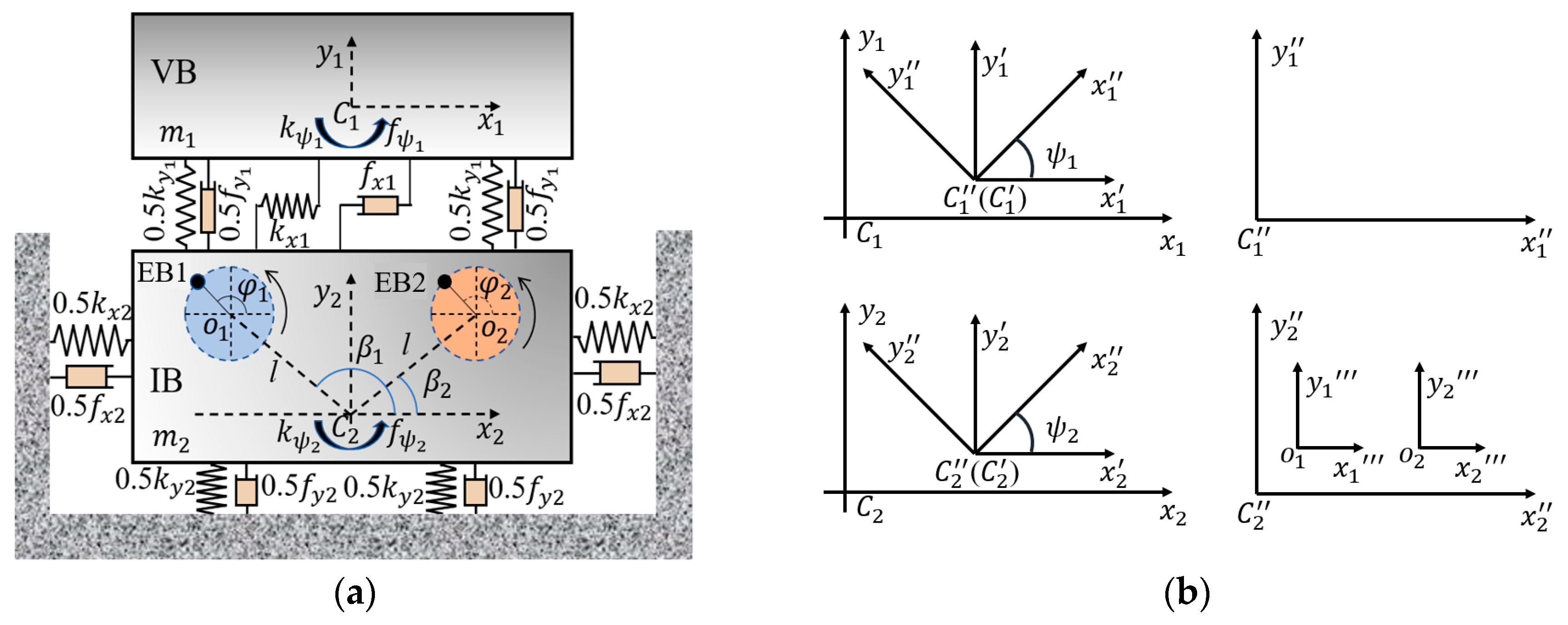
2. Dynamic Equation
3. Vibration Responses
4. Vibration Characters
4.1. Natural Frequency
4.2. Vibration Absorption Coefficient
5. Triple-Frequency Synchronization Condition and Stability Criterion
5.1. Self-Synchronization Condition
5.2. Stability Criterion
6. Numerical Analysis
6.1. Vibration Absorption Ability
6.2. Vibration Property
6.3. Stability Criterion
6.4. Stable Phase Difference
7. Computer Simulation
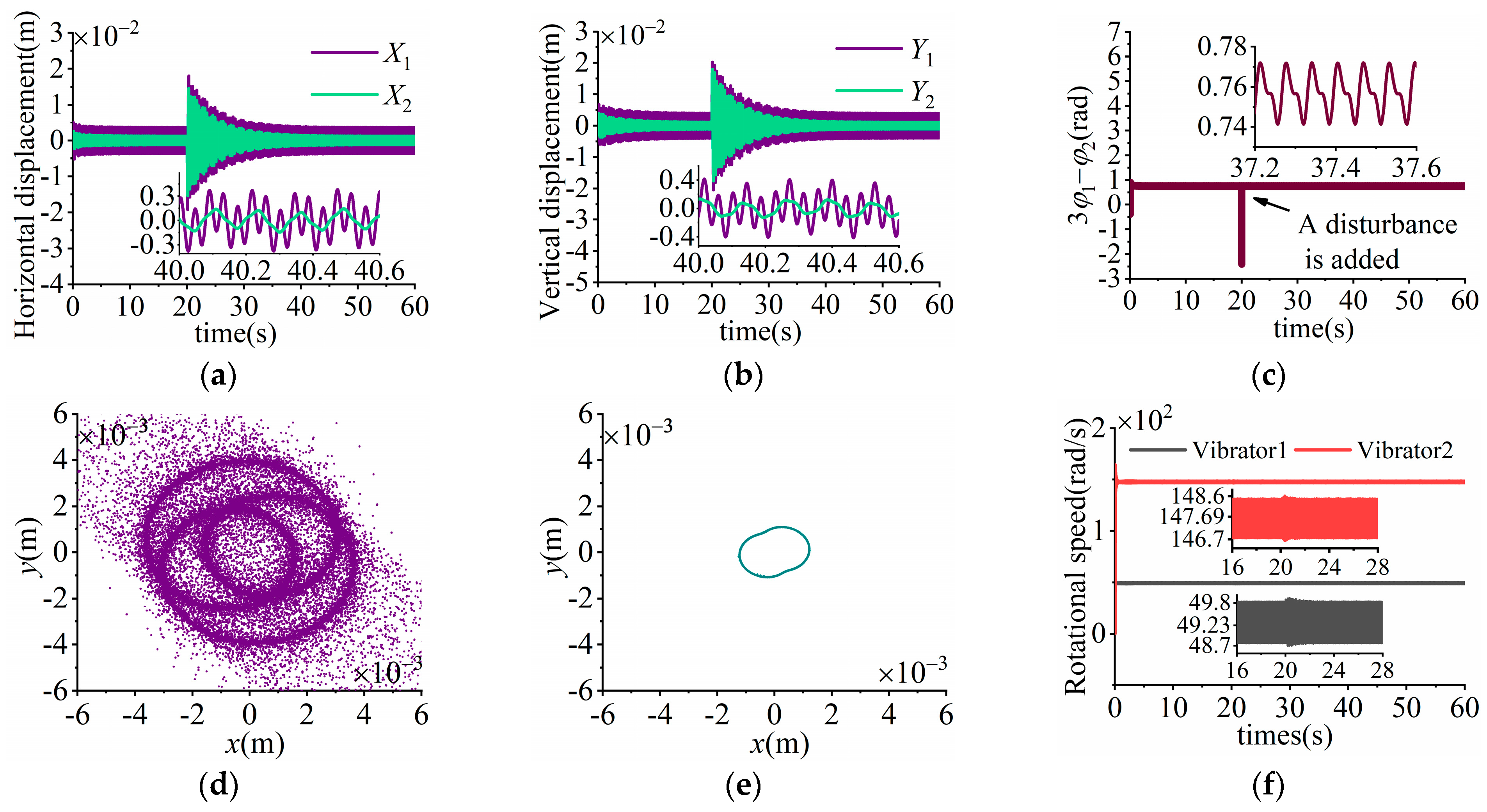
7.1. Simulation Results Under H1 > 0
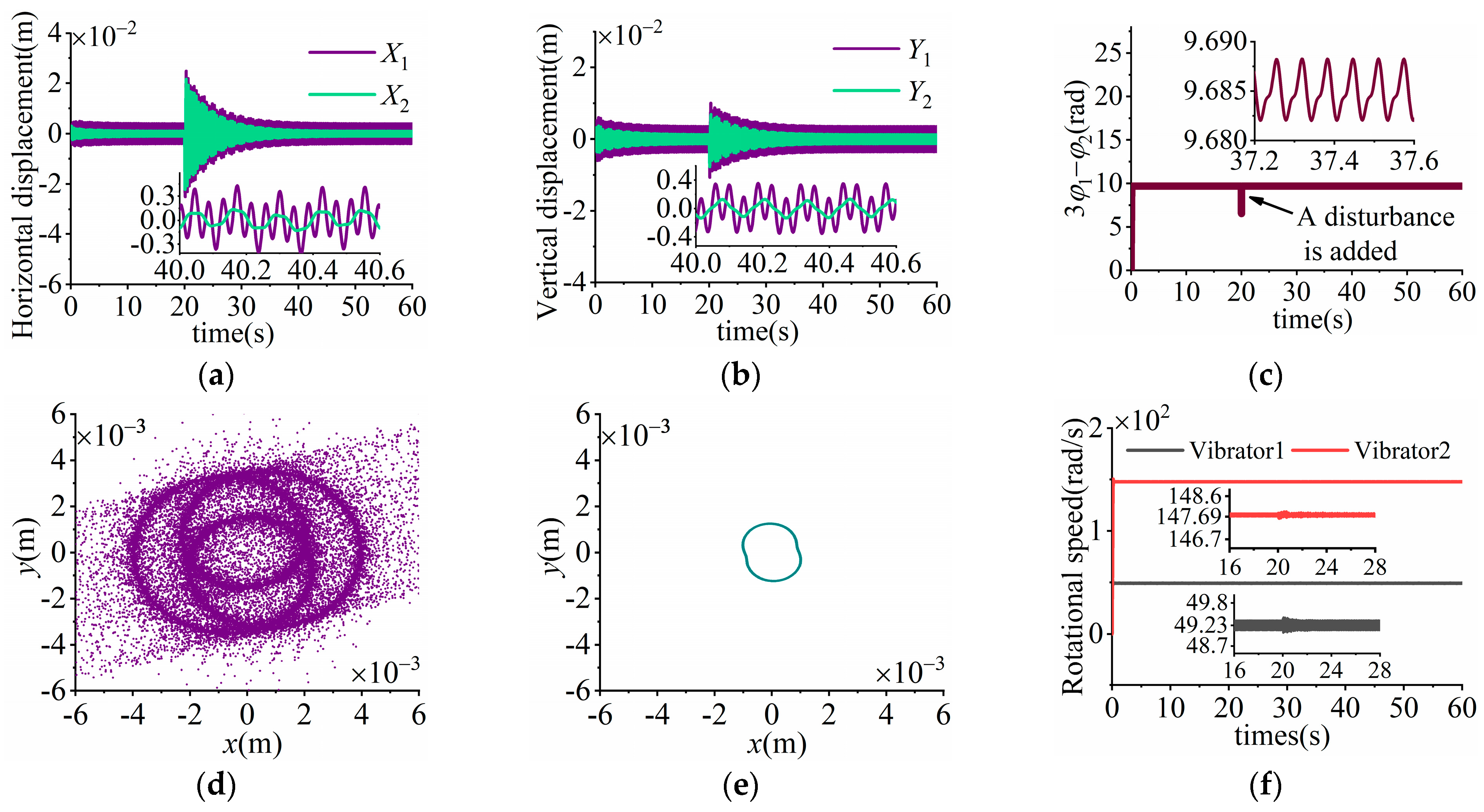
7.2. Simulation Results Under H1 < 0
7.3. Result Analysis
8. Conclusions
- (1)
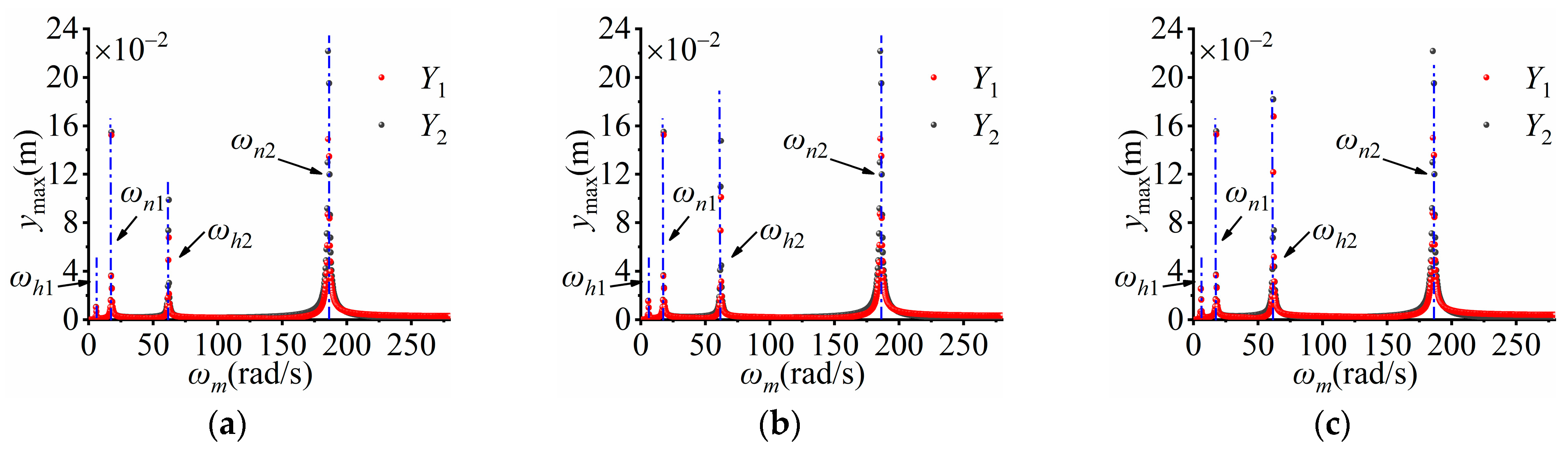
- In the near-resonance region of the triple-frequency anti-resonance system, two absorption zones are observed. When the mass of the low-frequency EB is constant, the vibration absorption capacity in the low-frequency absorption zone is proportional to a21 (the mass ratio of the EBs). Conversely, the vibration absorption capacity in the high-frequency absorption zone is inversely proportional to a21.
- (2)
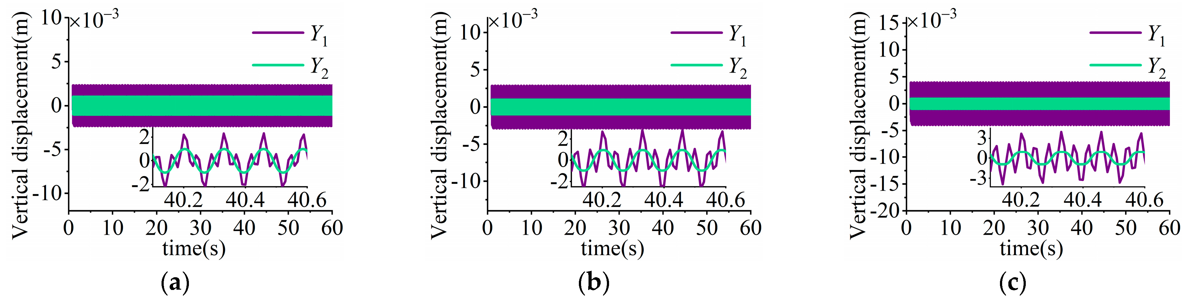
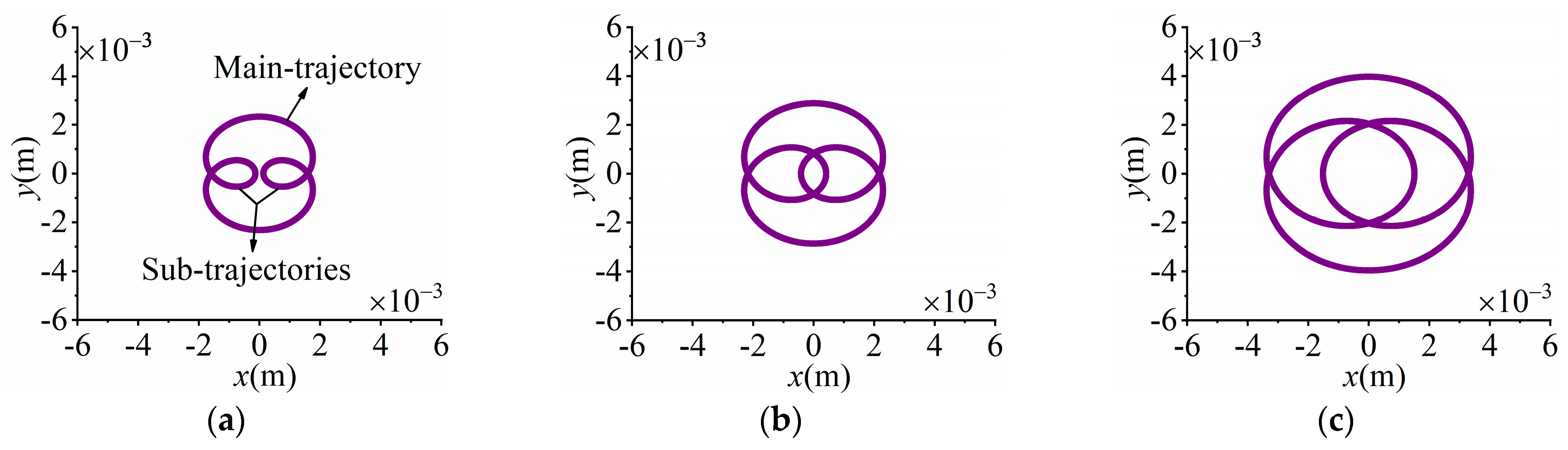
- During a single vibrational cycle, the number of peaks presented in the curve of the displacement is consistent with the frequency multiple, which indicates that the number of closed roundabout trajectories in the VB trajectory is equivalent to the multiple of the disturbance frequency. In this case, the working trajectory of the triple-frequency excitation vibration system can be characterized as the superposition of three closed roundabout trajectories.
- (3)
- When the mass of low-frequency EB remains constant, the influence of a21 on the magnitude of the natural frequency is considered negligible; however, the amplitude of the system is significantly impacted, i.e., the amplitude is increased with an increasing a21. In addition, the magnitude of TSR is also affected by a21, and larger values of a21 result in greater values of TSR.
- (4)
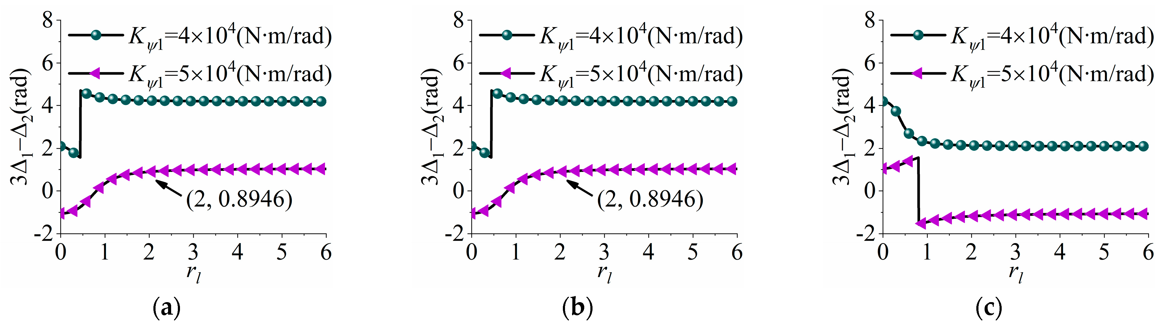
- Two solutions of phase difference exist in triple-frequency synchronization: one is stable and the other is unstable. The stability range is greatly affected by the rotational stiffness of bodies. In addition, when rl < 2, SPD is significantly influenced by rl; however, when rl > 2, the value of the SPD remains almost constant.
- (5)
- The validity of the adopted theoretical method and the feasibility of triple-frequency anti-resonance and synchronization characteristics are verified through theoretical comparative analysis, numerical qualitative analysis, and dynamical simulation.
Author Contributions
Funding
Data Availability Statement
Conflicts of Interest
Nomenclature
| r | Eccentric radius of each EB; |
| moi | Mass of EB installed on motor i, i = 1, 2; |
| φi | The instantaneous phase of EB i, i = 1, 2; |
| Δi | The relative phase of the EB i, i = 1, 2; |
| Mj | The mass of mass body j and its components, j = 1, 2; |
| ηi | Ratio of mass between EB i and total mass of the mechanical structure, i = 1, 2; |
| Joi | The moment of inertia of EB i, i = 1, 2; |
| ψ | Swing angles of mechanical structure; |
| n | Multiple of the high-frequency excitation force frequency relative to the fundamental frequency, n = 3; |
| kwi | Total stiffness coefficient of springs in w-direction, w = x, y, ψ; i = 1, 2; |
| fwi | Total damping coefficient of springs in w-direction, w = x, y, ψ; i = 1, 2; |
| fi | The friction coefficient between motor i and motor shaft i, i = 1, 2; |
| μwa | Amplitude amplification factors in the w-direction, w = x, y, ψ; a = 11, 12, 21, 22; |
| βi | The installation angle of motor i, i = 1, 2; |
| l | The installation distance of motor i, i = 1, 2; |
| Jj | Rotational inertia of body j in ψ-direction, j = 1, 2; |
| ζ | vibration absorption coefficient; |
| ωni | The i-th order natural frequency of the system, i = 1, 2; |
| ωhi | The i-th order resonance frequency of the high-frequency motor, i = 1, 2; |
| ωm | Excitation frequency of motors; |
| nwj | Ratio of natural frequency to excitation frequency in w-direction, w = x, y, ψ, j = 1, 2; |
| ε | Small parameter form of ηi; |
| Teoi | Electromagnetic torque of motor i, i = 1, 2; |
| ; | |
| ; | |
| M | Mass-coupling matrix of the system; |
| K | Stiffness-coupling matrix of the system; |
| VB | Vibration body; |
| IB | Isolation body; |
| EB | Abbreviation of ‘eccentric block’; |
| TSR | Abbreviation of ‘Trajectory size ratio’; |
Appendix A
Appendix B
References
- Lyan, I.; Panovko, G.; Shokhin, A. Creation and verification of a spatial mathematical model of a vibrating machine with two self-synchronizing unbalanced exciters. J. Vibroeng. 2021, 23, 1524–1534. [Google Scholar] [CrossRef]
- Sislian, R.; Cotta, R.S.; Barbosa, R.Y.M.; Barbosa, V.P.; Gedraite, R.; Guedes, M.P. Modeling of fluid content in vibratory screening residual solids using artificial neural networks. J. Eng. Exact Sci. 2025, 11, 21481. [Google Scholar] [CrossRef]
- Shokhin, A.E.; Krestnikovskii, K.V.; Nikiforov, A.N. On self-synchronization of inertial vibration exciters in a vibroimpact three-mass system. IOP Conf. Ser Mater. Sci. Eng. 2021, 1129, 012041. [Google Scholar] [CrossRef]
- Hou, Y.; Fang, P. Investigation for synchronization of a rotor-pendulum system considering the multi-DOF vibration. Shock. Vib. 2016, 2016, 8641754. [Google Scholar] [CrossRef]
- Strogatz, S. Exploring complex networks. Nature 2001, 410, 268–276. [Google Scholar] [CrossRef]
- Blekhman, I.I. Synchronization in Science and Technology; ASME Press: New York, NY, USA, 1988. [Google Scholar]
- Blekhman, I.I. Vibrational Mechanics; World Scientific: Singapore, 2000. [Google Scholar]
- Blekhman, I.I.; Fradkov, A.L.; Nijmeijer, H.; Pogromsky, A.Y. On self-synchronization and controlled synchronization. Syst. Control Lett. 1997, 31, 299–305. [Google Scholar] [CrossRef]
- Paz, M.; Cole, J.D. Self-synchronization of two unbalanced rotors. ASME J. Vib. Acoust. 1992, 114, 37–41. [Google Scholar] [CrossRef]
- Paz, M.; Morris, J.M. The use of vibration for material handling. ASME J. Eng. Ind. 1974, 96, 735–740. [Google Scholar] [CrossRef]
- Zhang, X.; Wen, B.; Zhao, C. Vibratory synchronization transmission of a cylindrical roller in a vibrating mechanical system excited by two exciters. Mech. Syst. Signal Process 2017, 6, 88–103. [Google Scholar] [CrossRef]
- Zhang, X.; Wen, B.; Zhao, C. Synchronization of three non-identical coupled exciters with the same rotating directions in a far-resonant vibrating system. J. Sound. Vib. 2013, 332, 2300–2317. [Google Scholar] [CrossRef]
- Zhang, X.; Gao, Z.; Yue, H.; Cui, S.; Wen, B. Stability of a multiple rigid frames vibrating system driven by two unbalanced rotors rotating in opposite directions. IEEE Access 2019, 7, 123521–123534. [Google Scholar] [CrossRef]
- Fang, P.; Hou, Y. Synchronization characteristics of a rotor-pendula system in multiple coupling resonant systems. Proc. Inst. Mech. Eng, Part. C J. Mech. Eng. Sci. 2018, 232, 1802–1822. [Google Scholar] [CrossRef]
- Fang, P.; Wang, Y.; Hou, Y.; Wu, Y. Synchronous control of multi-motor coupled with pendulum in a vibration system. IEEE Access 2020, 8, 51964–51975. [Google Scholar] [CrossRef]
- Fang, P.; Hou, Y.; Du, M.J. Synchronization behavior of a triple-rotor-pendula system in a dual-super-far resonance system. Proc. Inst. Mech. Eng, Part. C J. Mech. Eng. Sci. 2019, 233, 1620–1640. [Google Scholar] [CrossRef]
- Balthazar, J.M.; Palacios Felix, J.L.; MLRF Brasil, R. Some comments on the numerical simulation of self-synchronization of four non-ideal exciters. Appl. Math. Comput. 2005, 164, 615–625. [Google Scholar] [CrossRef]
- Balthazar, J.M.; Palacios Felix, J.L.; MLRF Brasil, R. Short comments on self-synchronization of two non-ideal sources supported by a flexible portal frame structure. J. Vib. Control 2004, 10, 1739–1748. [Google Scholar] [CrossRef]
- Kong, X.; Chen, C.; Wen, B. Composite synchronization of three eccentric rotors driven by induction motors in a vibrating system. Mech. Syst. Signal Process 2018, 102, 158–179. [Google Scholar] [CrossRef]
- Kong, X.; Zhou, C.; Wen, B. Composite synchronization of four exciters driven by induction motors in a vibration system. Meccanica 2020, 55, 2107–2133. [Google Scholar] [CrossRef]
- Zou, M.; Wang, Y.; Zhu, W.; Wang, Y.; Xie, D.; Kong, C.; Tang, S. Counter-rotating synchronization theory and experiment of tri-rotor actuated with dual-frequency considering adaptive global sliding mode control strategy. Mech. Syst. Signal Process 2025, 223, 111820. [Google Scholar] [CrossRef]
- Zhang, X.; Zhang, X.; Zhang, C.; Wang, Z.; Wen, B. Double and triple-frequency synchronization and their stable states of the two co-rotating exciters in a vibrating mechanical system. Mech. Syst. Signal Process 2021, 154, 107555. [Google Scholar] [CrossRef]
- Zhang, X.; Zhang, X.; Hu, W.; Zhang, W.; Chen, W.; Wang, Z.; Wen, B. Theoretical, numerical and experimental studies on multi-cycle synchronization of two pairs of reversed rotating exciters. Mech Syst Signal Process 2022, 167, 108501. [Google Scholar] [CrossRef]
- Zhang, X.; Zhang, W.; Chen, W.; Zhang, X.; Wang, Z.; Wen, B. Theoretical, numerical and experimental studies on time-frequency synchronization of the three exciters based on the asymptotic method. J. Vib. Eng. Technol. 2022, 10, 1091–1109. [Google Scholar] [CrossRef]
- Li, X.; Shen, T. Dynamic performance analysis of nonlinear anti-resonance vibrating machine with the fluctuation of material mass. J. Vibroeng. 2016, 18, 978–988. [Google Scholar] [CrossRef]
- Fang, P.; Sun, H.; Zou, M.; Peng, H.; Wang, Y.M. Self-synchronization and vibration isolation theories in an anti-resonance system with dual-motor and double-frequency actuation. J. Vib. Eng. Technol. 2022, 10, 409–424. [Google Scholar] [CrossRef]
- Sun, H.; Fang, P.; Peng, H.; Zou, M.; Xu, Y. Theoretical, numerical and experimental studies on double-frequency synchronization of three exciters in a dynamic vibration absorption system. Appl. Math. Model. 2022, 111, 384–400. [Google Scholar] [CrossRef]
- Kang, W.; Hou, Y.; Xu, X.; Hou, D.; Fang, P.; Song, W.; Li, X.; Chen, W.; Lu, C. Synchronization analysis of a four-motor excitation with torsion spring coupling vibrating system. Appl. Math. Model. 2025, 138 Pt A, 115766. [Google Scholar] [CrossRef]


| VB | IB | Vibrator 1/Vibrator 2 |
|---|---|---|
| M1 = 60 (kg) | M2 = 60~120 (kg) | m1 = 3 (kg) |
| kx1 = 0~3 × 10⁶ (N/m) | kx2 = 47,300 (N/m) | m2 = 1.2~3 (kg) |
| ky1 = 0~3 × 10⁶ (N/m) | ky2 = 47,300 (N/m) | β1 = π/6 or π/4 or π/3 (rad) |
| kψ1 = 0~11 × 104 (N∙m/rad) | kψ2 = 0~1 × 10⁵ (N∙m/rad) | β2 = π − β1 |
| J1 = 30 (kg∙m2) | J2 = 60 (kg∙m2) | rl = 0~6 |
| \ | \ | r = 0.05 (m) |
| Parameters of Vibrator | Vibrator 1 | Vibrator 2 |
|---|---|---|
| Nominal power | 3.7 × 10⁴ (VA) | 3.7 × 10⁴ (VA) |
| Power frequency | 15.8323 (Hz) | 47.5006 (Hz) |
| Rated velocity | 470 (r/min) | 1410 (r/min) |
| Pole pairs | 2 | 2 |
| Mass | m1 = 3 (kg) | m2 = 3 (kg) |
| Project | Theory Analysis | Simulation | Absolute Error | Relative Error |
|---|---|---|---|---|
| Simulation under H1 > 0 | 0.8946 rad | 0.76 rad | 0.1346 | 2.1422% |
| Simulation under H1 < 0 | 3.334 rad | 3.402 rad | 0.068 | 1.0823% |
Disclaimer/Publisher’s Note: The statements, opinions and data contained in all publications are solely those of the individual author(s) and contributor(s) and not of MDPI and/or the editor(s). MDPI and/or the editor(s) disclaim responsibility for any injury to people or property resulting from any ideas, methods, instructions or products referred to in the content. |
© 2025 by the authors. Licensee MDPI, Basel, Switzerland. This article is an open access article distributed under the terms and conditions of the Creative Commons Attribution (CC BY) license (https://creativecommons.org/licenses/by/4.0/).
Share and Cite
Hou, D.; Liang, Z.; Zhang, Z.; Wang, Z. Studies on Vibration and Synchronization Characteristics of an Anti-Resonance System Driven by Triple-Frequency Excitation. Machines 2025, 13, 534. https://doi.org/10.3390/machines13070534
Hou D, Liang Z, Zhang Z, Wang Z. Studies on Vibration and Synchronization Characteristics of an Anti-Resonance System Driven by Triple-Frequency Excitation. Machines. 2025; 13(7):534. https://doi.org/10.3390/machines13070534
Chicago/Turabian StyleHou, Duyu, Zheng Liang, Zhuozhuang Zhang, and Zihan Wang. 2025. "Studies on Vibration and Synchronization Characteristics of an Anti-Resonance System Driven by Triple-Frequency Excitation" Machines 13, no. 7: 534. https://doi.org/10.3390/machines13070534
APA StyleHou, D., Liang, Z., Zhang, Z., & Wang, Z. (2025). Studies on Vibration and Synchronization Characteristics of an Anti-Resonance System Driven by Triple-Frequency Excitation. Machines, 13(7), 534. https://doi.org/10.3390/machines13070534