A Novel Rapid Design Framework for Tooth Profile of Double-Circular-Arc Common-Tangent Flexspline in Harmonic Reducers

Abstract

Due to its small size, high transmission ratio and precision, the harmonic reducer is widely used. The design of the flexspline tooth profile is crucial for the transmission accuracy and service life of harmonic reducers. However, the numerous design parameters and the lack of a unified design standard for the flexspline tooth profile make it challenging to accurately determine these parameters. This can lead to issues such as tooth profile interference and excessive stress on the gear teeth during transmission. To address these issues, we propose a novel rapid design framework for the tooth profile of a double-circular-arc common-tangent flexspline in harmonic reducers. Firstly, the mathematical formula for the flexspline tooth profile with a double-circular-arc common-tangent and its conjugate circular spline tooth profile is derived. Then, two-dimensional and three-dimensional parametric finite element models of the harmonic reducer are established, and radial and axial profile modifications of the flexspline are carried out. Based on the parametric two-dimensional finite element model of the harmonic reducer, the optimized Latin hypercube experimental design method is employed to determine the flexspline tooth profile parameters. The method proposed can be implemented using Python language code and integrated into the Abaqus 2019 software, offering the advantage of meeting the requirements for rapid engineering development. Finally, a case study is presented to verify the effectiveness of the proposed design method.

1. Introduction

The harmonic reducer primarily consists of a flexspline, a circular spline, and a wave generator. After the wave generator is installed, the flexspline undergoes elastic deformation, causing its teeth to engage with the teeth of the circular spline. As the wave generator rotates, the engagement point of the flexspline moves circumferentially, resulting in the flexspline rotating relative to the circular spline [1,2,3]. This unique working principle enables the harmonic drive to achieve a high reduction ratio, low backlash, and high torque transmission. Consequently, it is widely used in robotics [4,5,6], aerospace [7], and precision machinery [8].

The design of the flexspline tooth profile significantly impacts the transmission accuracy, load capacity, transmission efficiency, and service life of the harmonic drive. Scholars have conducted extensive research on the effects of different types of flexspline tooth profiles on harmonic transmission. Dong et al. [9] adopted the involute as the flexspline tooth profile, establishing a kinematic model of harmonic transmission based on the assumption of the invariance of the flexspline neutral layer curve [10] and conjugate theory. Chen et al. [11] used a double-circular-arc common-tangent curve as the flexspline tooth profile, analyzed the impact of double-circular-arc common-tangent profile parameters on conjugate meshing accuracy, and proposed an accurate calculation method for the double-circular-arc common-tangent curve tooth profile. Additionally, cycloidal profiles have also been utilized in the design of harmonic transmissions [12,13].

Beyond the flexspline tooth profile, the geometry of the wave generator exerts a significant influence on the meshing characteristics and overall performance of harmonic drive systems. Among the various configurations, the cam-type wave generator is the most prevalently adopted in practice. Its profile is commonly constructed using standard elliptical curves [14], double eccentric circles [15], cosine curves [16], or split-cam configurations [10]. Extensive research efforts have been devoted to investigating the impact of wave generator profile design on system performance. For instance, Gravagno et al. [17] examined the effect of wave generator geometry on pure kinematic error, demonstrating that the Resàl curve yields the lowest error among the compared profiles. Sahoo and Maiti [18] analyzed the stress distribution induced in the flexspline due to wave generator insertion, highlighting the critical role of wave generator shape in stress management. From the perspective of design methodology, Li et al. [19] proposed a multi-objective optimization framework based on the Fourier series representation of the support function, aiming to simultaneously minimize the maximum circumferential stress in the flexspline, the curvature deviation of the neutral line, and the pure kinematic error resulting from wave generator engagement.

During the actual operation of the harmonic drive, the flexspline undergoes very complex elastic deformation. For flexsplines with different tooth profile parameters, it is challenging to accurately express their dynamic meshing performance, such as the dynamic tooth engagement stress, using a unified mathematical model. Finite element simulation analysis is a more direct and convenient method to obtain the dynamic meshing performance of the harmonic drive and has been widely adopted. Rhéaume et al. [20] established a three-dimensional finite element simulation model of the harmonic drive and studied the torsional stiffness of the harmonic transmission. Song et al. [21] simplified the harmonic drive to a two-dimensional planar transmission model, establishing a two-dimensional finite element simulation model of the harmonic transmission and analyzing the impact of tooth profile parameters on tooth shape and maximum stress during meshing. Pacana et al. [22] used ABAQUS software to establish a simplified two-dimensional finite element model of the harmonic drive, analyzing the impact of four different types of wave generators on harmonic drive accuracy. Subsequently, Song et al. [23] established a three-dimensional finite element simulation model of the harmonic drive with double-circular-arc common-tangent tooth profile and proposed a design method of three-dimensional conjugate tooth surface.

Due to the significant impact of flexspline tooth profile parameters on the dynamic performance of harmonic drives, scholars have conducted research on optimizing these parameters to find suitable profiles. The computational volume of the three-dimensional finite element dynamic simulation model of harmonic drives is large, making multiple iterative calculations difficult. To reduce the computational load, Cheng and Chen [24] established two-dimensional and three-dimensional static simulation models of harmonic drives and optimized the tooth profile parameters based on the stress magnitude at a specific contact location. Kayabasi and Erzincanli [25] and León [26] developed approximate response surface optimization models for the dynamic performance of harmonic drives, enabling rapid iterative optimization. However, there are still certain errors in the prediction accuracy of the response surface models compared with the finite element simulation models.

To address the issue of the large computational volume in iterative calculations of finite element dynamic simulation models, we establish a parametric two-dimensional dynamic finite element model of a harmonic drive with a double-circular-arc common-tangent flexspline tooth profile. An optimized Latin hypercube experimental design method is employed to sample and calculate all sample points within the design range of each flexspline parameter. The sample point with the minimum peak meshing stress is selected to determine the tooth profile parameters of the flexspline. This method allows for the rapid determination of the tooth profile parameters of the flexspline and circular spline during the design of harmonic drives, and it also facilitates the obtaining of a three-dimensional flexspline shape with both radial and axial profile modifications. The method proposed can be implemented using Python code and integrated into the Abaqus software, offering the advantage of meeting the requirements for rapid engineering development.

This paper is organized as follows: First, based on the assumption of the invariance of the neutral layer, the mathematical expressions of double-circular-arc common-tangent flexspline tooth profile and its conjugate circular spline tooth profile are derived in detail. Second, a parametric finite element dynamic simulation model of the harmonic drive is established, and a novel rapid design method for the flexspline tooth profile is proposed. Third, a numerical example is provided to verify the effectiveness of the proposed method. Finally, the conclusions are presented.

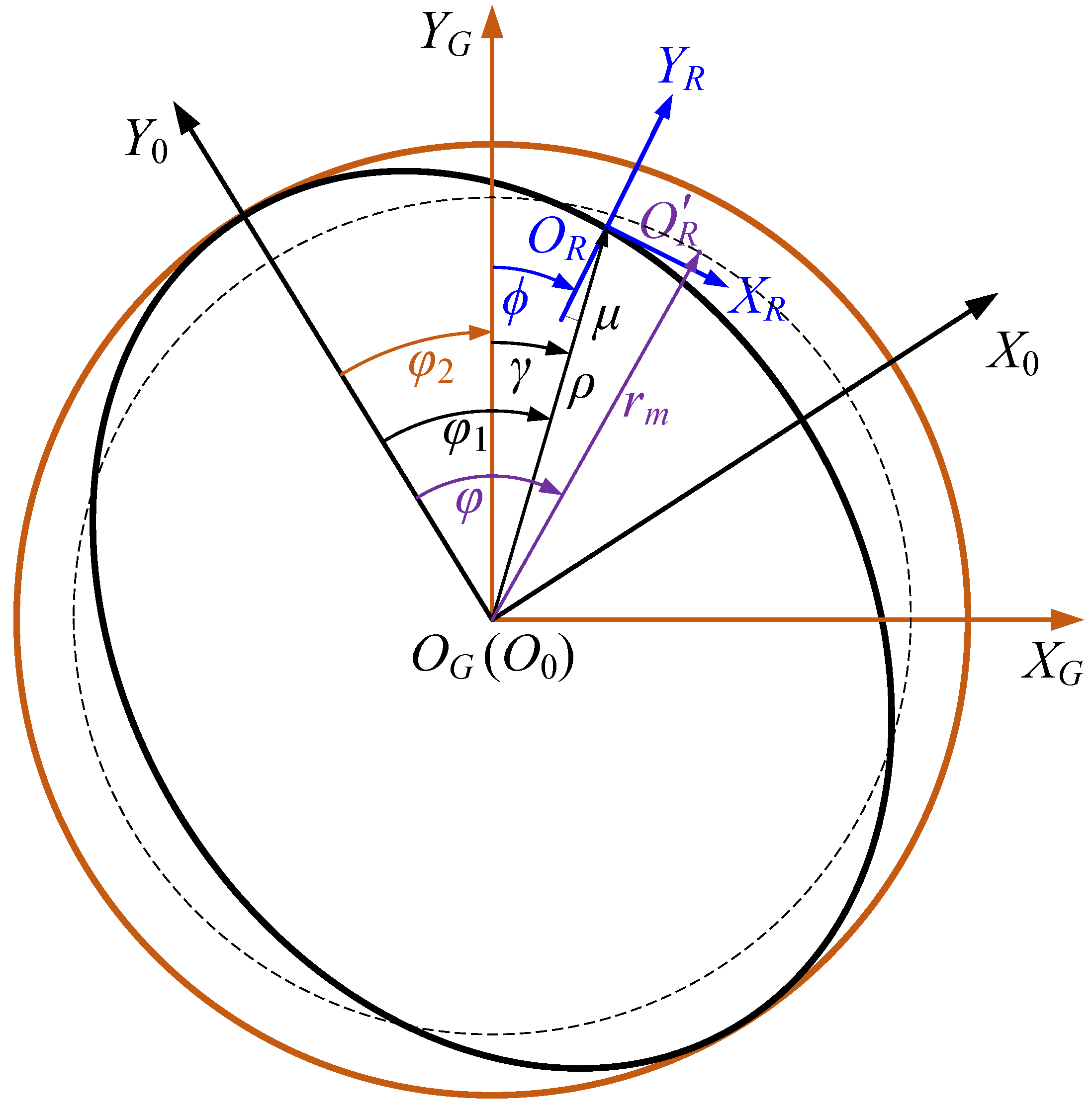
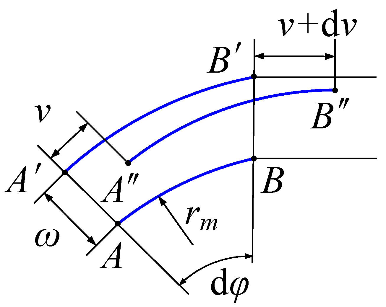
2. Mathematical Derivation of Double-Circular-Arc Common-Tangent Flexspline Tooth Profile and Its Conjugate Circular Spline Tooth Profile

Harmonic drives typically do not use involute gear profiles, but instead adopt non-involute profiles such as double-arc or cycloidal tooth shapes. This preference arises from the fundamental differences in operating conditions. Involute gears are based on the assumption of rigid bodies and constant center distances, offering pure rolling contact under such conditions. However, harmonic drives involve elastic deformation of the flexspline induced by the wave generator, resulting in a time-varying elliptical shape. This leads to significant tooth surface sliding and deformation, rendering the advantages of involute gearing ineffective. Moreover, involute profiles are insensitive to variations in center distance, while harmonic drives require dynamic changes in center distance to function properly. In contrast, non-involute profiles can be more easily tailored to the deformation characteristics of the flexspline. They enable higher contact ratios, smoother load distribution, and improved fatigue resistance through local profile modification. Additionally, non-involute profiles offer greater design flexibility, allowing engineers to customize local curvature and tooth geometry to better match the contact path, minimize stress concentrations, and enhance overall transmission performance. Therefore, this study adopts the double-arc tooth profile.

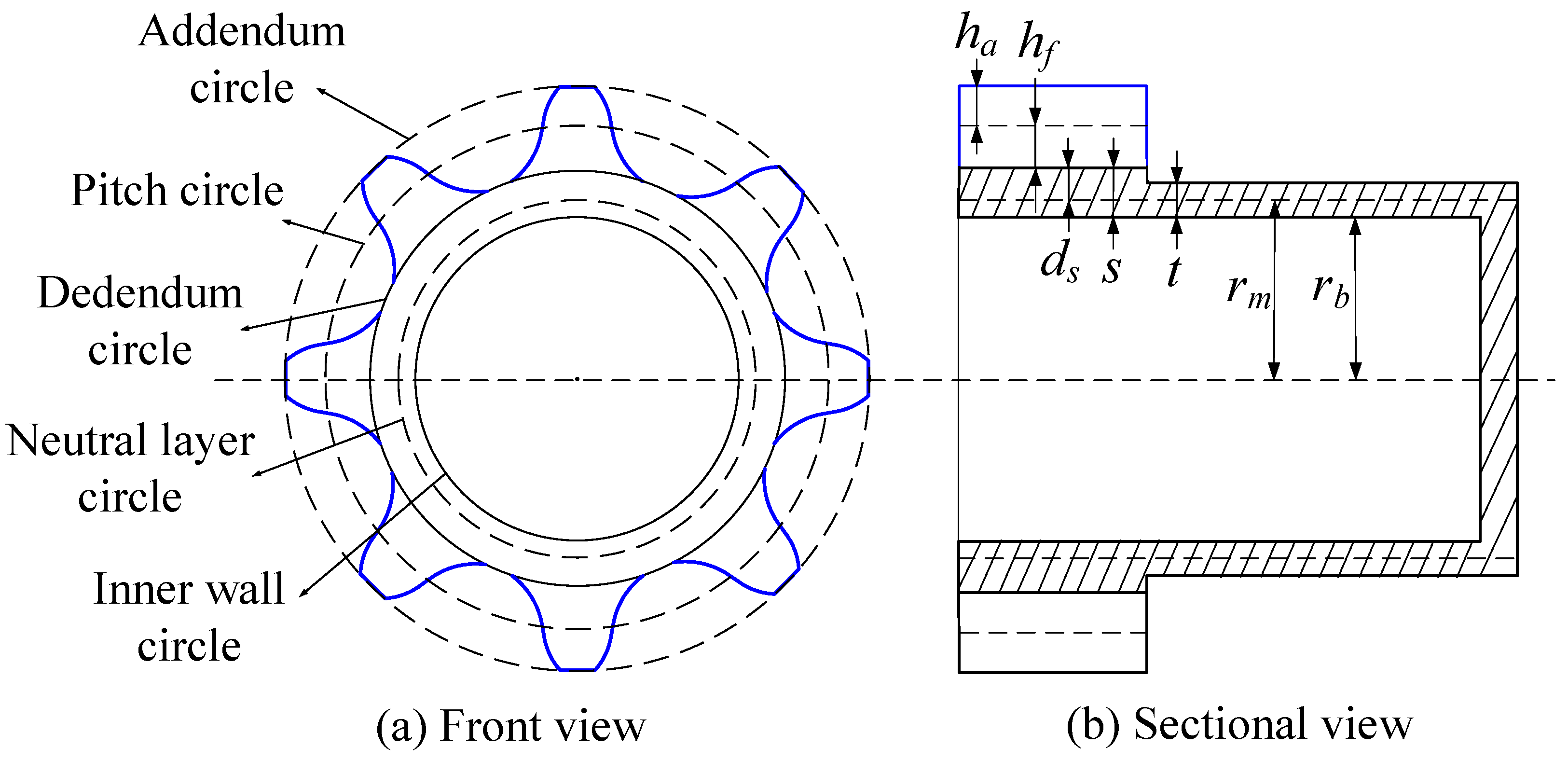
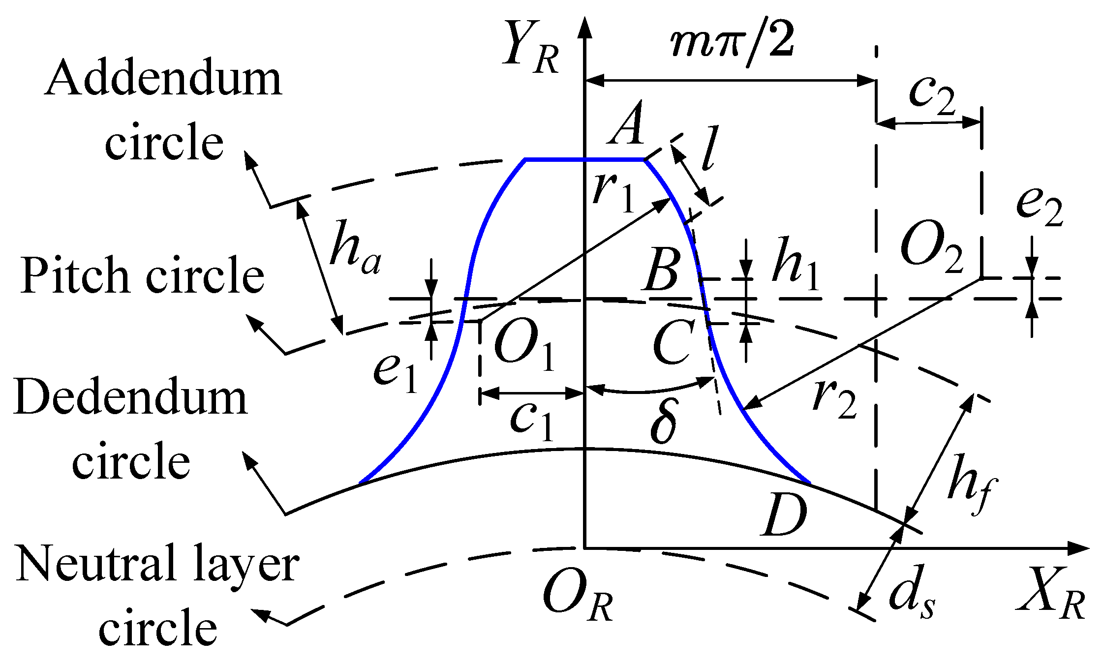
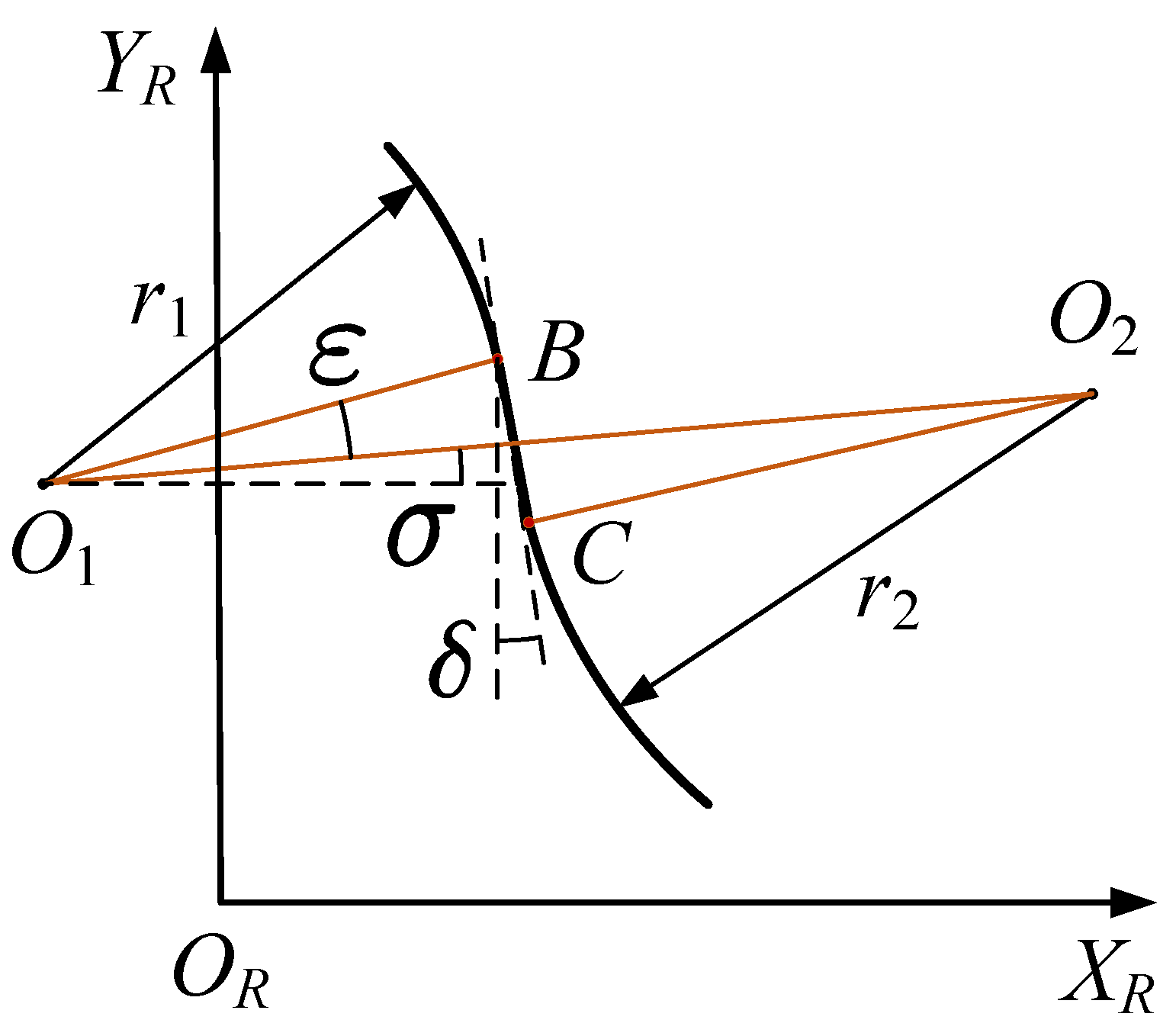
2.1. Mathematical Derivation of Double-Circular-Arc Common-Tangent Flexspline Tooth Profile

To clearly describe the flexspline and its tooth profile, the parameters are labeled on the schematic diagram of the flexspline using a cup-type flexspline as an example, as shown in Figure 1. Figure 1a is a front view schematic of the flexspline, with the addendum circle, pitch circle, dedendum circle, neutral layer circle, and inner wall circle of the flexspline shown from the outside to the inside along the radial direction. The neutral layer circle is located at the central layer of the wall thickness of the flexspline cup. Figure 1b is a sectional view schematic of the flexspline, where $h_a$ represents the addendum height, $h_f$ the dedendum height, $d_s$ the distance from the dedendum circle to the neutral layer, s the tooth ring wall thickness, t the flexspline cup wall thickness, $r_m$ the radius of the neutral layer circle, and $r_b$ the radius of the inner wall circle of the flexspline. So

$$d_s=s-t/2.$$

(1)

Figure 1. Flexspline parameters schematic diagram.

The double-circular-arc common-tangent flexspline tooth profile consists of two arc segments and their tangent line. Its basic profile is shown in Figure 2, where segment $AB$ is the convex arc segment, segment $BC$ is the tangent line segment, and segment $CD$ is the concave arc segment. To mathematically represent each segment of the tooth profile, the flexspline coordinate system is established as follows. The $Y_R$ axis is the symmetry axis of one of the flexspline teeth, and the $X_R$ axis is tangent to the neutral layer circle of the flexspline, with the tangent point $O_R$ serving as the origin of the coordinate system. The radius length of arc $AB$ is $r_1$, with its center at point $O_1$. The distance from point $O_1$ to the $Y_R$ axis is $c_1$, and the distance to the tangent of the pitch circle is $e_1$. Similarly, the radius length of arc $CD$ is $r_2$, with its center at point $O_2$. The distance from point $O_2$ to the $Y_R$ axis is $c_2$, and the distance to the tangent of the pitch circle is $e_2$. The module of the gear is m. The longitudinal length of the tangent line segment $BC$ is $h_1$, and the angle between $BC$ and the $Y_R$ axis is $\delta$, also known as the common tangential inclination angle.

Figure 2. Parameters of flexspline tooth profile schematic diagram.

The single-sided tooth profile of the flexspline starts from point A on the addendum circle and ends at point D on the dedendum circle. Let $l_1$ represent the length along the tooth profile from point A to any arbitrary point on the profile. The coordinates of points on the convex arc segment $AB$ in the $\{O_R-X_R-Y_R\}$ coordinate system can be expressed as follows,

$$\left\{\begin{array}{c}{x}_{AB}^R=r_{1}cos\left(\alpha -{\displaystyle \frac{l}{r_1}}\right)+x_1^R\hfill \\ y_{AB}^R=r_{1}sin\left(\alpha -{\displaystyle \frac{l}{r_1}}\right)+y_1^R\hfill \end{array},l\in (0,l_1),\right.$$

(2)

where $\left(x_1^R,y_1^R\right)$ represents the coordinates of the center point $O_1$, and

$$\begin{array}{cc}\hfill \alpha & =arcsin\left({\displaystyle \frac{h_a+e_1}{r_1}}\right),\hfill \\ \hfill x_1^R& =-c_1,\hfill \\ \hfill y_1^R& =d_s+h_f-e_1,\hfill \\ \hfill l_1& =r_1(\alpha -\delta ).\hfill \end{array}$$

(3)

The coordinates of points on the tangential segment $BC$ in the $\{O_R-X_R-Y_R\}$ coordinate system can be expressed as,

$$\left\{\begin{array}{c}{x}_{BC}^R=r_{1}cos\delta +x_1+(l-l_1)sin\delta \hfill \\ y_{BC}^R=r_{1}sin\delta +x_1+(l-l_1)cos\delta \hfill \end{array},l\in (l_1,l_2),\right.$$

(4)

where

$$l_2=l_1+{\displaystyle \frac{h_1}{cos\delta }}.$$

(5)

The coordinates of points on the concave arc segment $CD$ in the $\{O_R-X_R-Y_R\}$ coordinate system can be expressed as,

$$\left\{\begin{array}{c}{x}_{CD}^R=-r_{2}cos\left(\delta +{\displaystyle \frac{l-l_2}{r_2}}\right)+x_2^R\hfill \\ y_{CD}^R=r_{1}sin\left(\delta +{\displaystyle \frac{l-l_2}{r_2}}\right)+y_2^R\hfill \end{array},l\in (l_2,l_3),\right.$$

(6)

where $\left(x_2^R,y_2^R\right)$ represents the coordinates of the center point $O_2$, and

$$\begin{array}{cc}\hfill x_2^R& ={\displaystyle \frac{m\pi }{2}}+c_2,\hfill \\ \hfill y_2^R& =d_s+h_f+e_2,\hfill \\ \hfill l_3& =l_2+r_2\left(arcsin\left({\displaystyle \frac{e_2+h_f}{r_2}}\right)-\delta \right).\hfill \end{array}$$

(7)

The common tangential inclination angle $\delta$ and the longitudinal length $h_1$ of the tangent line are determined by the positions of the centers $O_1$ and $O_2$ of the two circles and their radii $r_1$ and $r_2$. The specific derivation is as follows.

As shown in Figure 3, let the distance between point $O_1$ and point $O_2$ be d,

$$d=\sqrt{{(y_1-y_2)}^2+{(x_1-x_2)}^2}.$$

(8)

Figure 3. Diagram of the common tangential inclination angle calculation.

Let the angle between line segment $O_{1}B$ and line segment $O_1{O}_2$ be $\epsilon$,

$$\epsilon =arccos\left({\displaystyle \frac{r_1+r_2}{d}}\right).$$

(9)

Let the angle between the line segment $O_1{O}_2$ and the $X_R$ axis be $\sigma$,

$$\sigma =arctan\left({\displaystyle \frac{y_1-y_2}{x_1-x_2}}\right).$$

(10)

Thus, the inclination angle $\delta$ of the tangent line can be obtained as

$$\delta =\epsilon +\sigma .$$

(11)

The vertical coordinates of points B and C in the $\{O_R-X_R-Y_R\}$ coordinate system are, respectively, given by

$$\begin{array}{cc}\hfill y_B^R& =r_{1}sin\delta +d_s+h_f-e_1,\hfill \\ \hfill y_C^R& =d_s+h_f+e_2-r_{2}sin\delta .\hfill \end{array}$$

(12)

The longitudinal length $h_1$ of the tangent line is given by

$$h_1=y_B^R-y_C^R.$$

(13)

2.2. Mathematical Derivation of the Conjugate Circular Spline Tooth Profile

During the transmission process of the harmonic drive, the flexspline undergoes complex spatial elastic deformation under the action of the wave generator, making it difficult to describe the kinematics of the tooth profile directly using mathematical formulas. Therefore, the following assumptions are made for the flexspline in the plane.

(1)

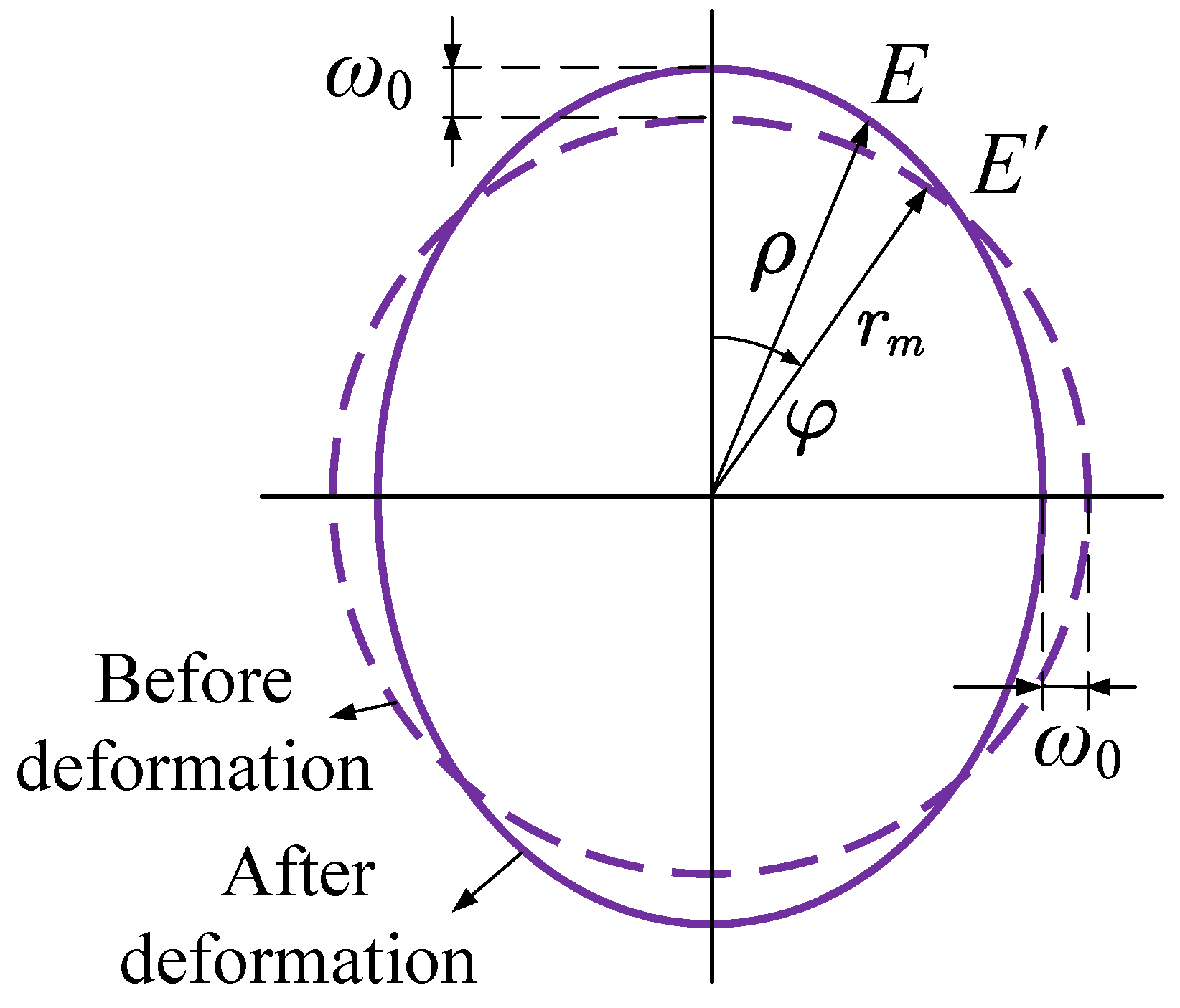
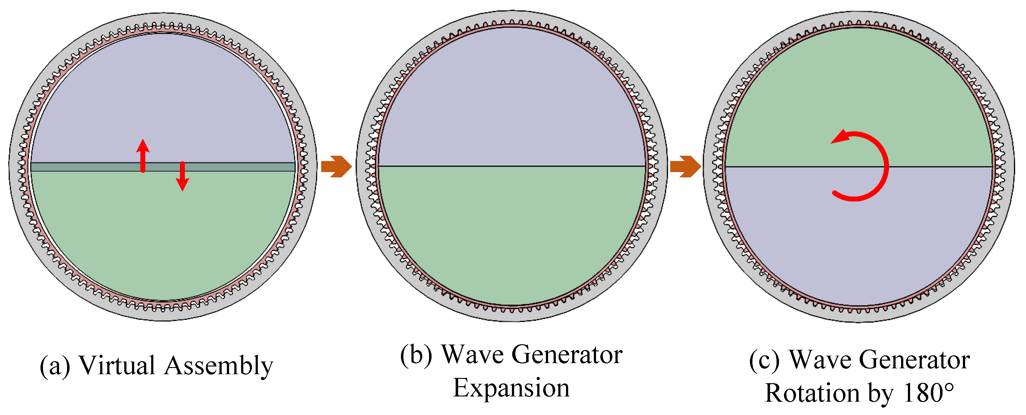
The circumference of the neutral layer circle, as shown in Figure 1, does not change before and after the wave generator is installed.

(2)

After the wave generator is installed into the flexspline, deformation occurs only in the part between the dedendum circle and the inner wall circle of the flexspline. This deformation is reflected only as changes in the tooth slots between adjacent teeth, with no deformation in the tooth portions of the flexspline.

(3)

The wave generator is considered a rigid body, and its shape changes are not considered during the transmission process.

(4)

After the wave generator is installed into the flexspline, the shapes of the addendum circle, pitch circle, dedendum circle, and inner wall circle of the flexspline are all consistent with the shape of the neutral layer circle, which are equidistant offset curves of the neutral layer curve.

Using a cosine-type wave generator as an example, Figure 4 shows a schematic diagram of the deformation of the flexspline’s neutral layer curve. The dashed line represents the curve before deformation, which is a circle, and the solid line represents the curve after deformation, which is a cosine curve. ${\omega }_0$ denotes the maximum radial deformation of the flexspline. Let point $E^{\prime }$ be a point on the neutral layer curve before deformation, and point E be the corresponding point after deformation. The radial vector $\rho$ of point E from the center after deformation can be expressed as

$$\rho =r_m+{\omega }_{0}cos2\phi ,$$

(14)

where $\phi$ is the angle between the radial vector formed by the undeformed endpoint $E^{\prime }$ and the center of the circle and the major axis after deformation.

Figure 4. Before and after deformation of the neutral layer curve.

We use the envelope method to design the tooth profile of the circular spline. The envelope method considers the elastic deformation of the flexspline as part of the conjugate motion and takes the envelope of the motion trajectory of the flexspline tooth profile in the circular spline coordinate system. This envelope curve is the tooth profile of the circular spline and is conjugate to the flexspline tooth profile. The following section explains how to use the envelope method to obtain the tooth profile of the circular spline.

To clearly describe the harmonic drive relationship, a harmonic drive angular relationship diagram, as shown in Figure 5, is established. The circular spline is fixed, the wave generator is the input, and the flexspline is the output. The fixed coordinate system $\{O_G-X_G-Y_G\}$ is established with the center of rotation of the circular spline as the origin $O_G$ and the vertical line passing through $O_G$ as $Y_G$. The moving coordinate system $\{O_0-X_0-Y_0\}$ is established with the center of rotation of the wave generator as the origin $O_0$ and the major axis of the wave generator as $Y_0$. Consistent with previous sections, the coordinate system $\{O_R-X_R-Y_R\}$ represents the moving coordinate system of the flexspline.

Figure 5. Harmonic drive angular relationship diagram.

In Figure 5, $\phi$ is consistent with the previous description, representing the angle between the undeformed endpoint of the flexspline and the $Y_0$ axis. ${\phi }_1$ is the angle between the deformed endpoint of the flexspline and the $Y_0$ axis, ${\phi }_2$ is the rotation angle of the wave generator. $\gamma$ is the rotation angle of the deformed endpoint of the flexspline, $\mu$ is the normal deformation angle, and $\varphi$ is the angle between the $Y_G$ axis and $Y_R$ axis. All angles are considered positive in the direction indicated in the diagram.

Under the action of the wave generator, the neutral layer curve of the flexspline mainly undergoes three types of deformation: radial deformation $\omega$, tangential deformation v, and normal deformation $\mu$. As shown in Figure 6, the unit arc length $AB$ deforms to $A^{\prime }{B}^{\prime }$, with the radial displacements at the endpoints being $\omega$ and $\omega +d\omega$. Therefore, the radial change in this unit arc length is

$$A^{\prime }{B}^{\prime }-AB=(r_m+\omega )d\phi -r_{m}d\phi =\omega d\phi ,$$

(15)

where $d\phi$ is the unit angular deformation of the neutral layer curve of the flexspline, and $d\omega$ is the unit change in radial displacement.

Figure 6. Unit arc deformation of the neutral layer curve.

The deformation equation for radial displacement can be expressed as

$$\omega =\rho -R_m.$$

(16)

Substituting Equation (14) into Equation (16) yields

$$\omega ={\omega }_{0}cos2\phi .$$

(17)

This unit arc length $A^{\prime }{B}^{\prime }$ further deforms to $A^{″}{B}^{″}$, with the tangential displacements at the endpoints being v and $v+dv$, respectively. Therefore, the tangential change in this unit arc length is

$$A^{″}{B}^{″}-A^{\prime }{B}^{\prime }=(v+dv)-v=dv,$$

(18)

where $dv$ is the unit change in tangential displacement.

According to the above assumptions of the harmonic drive, the length of the neutral layer curve of the flexspline does not change during deformation. Therefore, the sum of the radial and tangential changes in the unit arc length should equal zero, so

$$\omega d\phi +dv=0.$$

(19)

Thus, the expression for the tangential displacement deformation equation can be obtained as

$$v=-\int \omega d\phi =-{\displaystyle \frac{1}{2}}{\omega }_{0}sin\left(2\phi \right).$$

(20)

The normal deformation angle $\mu$ is very small and $r_m$ is much larger than $\omega$; according to differential geometry, $\mu$ can be obtained from the radial vector of the neutral layer curve of the flexspline,

$$\mu =arctan\left({\displaystyle \frac{\dot{\rho }}{\rho }}\right)=arctan\left({\displaystyle \frac{\dot{\rho }}{r_m+\omega }}\right)\approx -{\displaystyle \frac{1}{r_m}}{\displaystyle \frac{d\omega }{d\phi }}={\displaystyle \frac{2{\omega }_0}{r_m}}sin\left(2\phi \right),$$

(21)

where $\dot{\rho }$ is the derivative of $\rho$ with respect to $\phi$.

Since the length of the neutral layer curve of the flexspline remains unchanged before and after deformation, we have

$$r_m\phi ={\int }_0^{{\phi }_1}\sqrt{{\rho }^2+{\dot{\rho }}^2}d\phi \approx {\int }_0^{{\phi }_1}\rho d\phi .$$

(22)

Based on Equation (22), we obtain

$${\phi }_1=\phi -{\displaystyle \frac{{\omega }_{0}sin\left(2\phi \right)}{2r_m}}.$$

(23)

According to the transmission ratio relationship of the harmonic drive, we obtain

$${\displaystyle \frac{z_f}{z_c}}={\displaystyle \frac{{\phi }_2}{\phi }},$$

(24)

where $z_f$ is the number of teeth on the flexspline and $z_c$ is the number of teeth on the circular spline, we have

$${\phi }_2={\displaystyle \frac{z_f}{z_c}}\phi .$$

(25)

Therefore, the deformation angle $\gamma$ of the flexspline’s deformed endpoint can be obtained as

$$\gamma ={\phi }_1-{\phi }_2.$$

(26)

And the angle $\varphi$ between the $Y_G$ axis and $Y_R$ axis is

$$\varphi =\mu +\gamma .$$

(27)

To determine the motion trajectory of the flexspline tooth profile in the circular spline coordinate system, it is essentially a coordinate transformation of the points on the flexspline tooth profile. The transformation equations can be expressed as follows,

$$\left\{\begin{array}{c}{\mathbf{X}}_g=\mathbf{M}{\mathbf{X}}_r\hfill \\ \mathbf{M}=\left[\begin{array}{ccc}cos\varphi & sin\varphi & \rho sin\gamma \\ -sin\varphi & cos\varphi & \rho cos\gamma \\ 0& 0& 1\end{array}\right]\hfill \\ {\mathbf{X}}_r={\left[\begin{array}{c}{x}_r\\ y_r\\ 1\end{array}\right]}^T\hfill \\ {\mathbf{X}}_g={\left[\begin{array}{c}{x}_g\\ y_g\\ 1\end{array}\right]}^T\hfill \end{array}\right.$$

(28)

Here, ${\mathbf{X}}_r$ represents the position vectors of points on the flexspline tooth profile in the flexspline coordinate system $\{O_R-X_R-Y_R\}$, and ${\mathbf{X}}_g$ represents the position vectors of points on the flexspline tooth profile in the fixed coordinate system $\{O_G-X_G-Y_G\}$. $\mathbf{M}$ represents the transformation matrix. From Equation (28), we have the following:

$$\left\{\begin{array}{c}{x}_g=x_{r}cos\varphi +y_{r}sin\varphi +\rho sin\gamma \hfill \\ y_g=-x_{r}sin\varphi +y_{r}cos\varphi +\rho cos\gamma \hfill \end{array}\right.$$

(29)

Based on the above transformation relationship, by continuously rotating $\phi$ in the range of $[-\pi /2,\pi /2]$, the motion trajectory of the flexspline can be obtained. According to the envelope conjugate principle, the conjugate circular spline tooth profile must satisfy the following:

$${\displaystyle \frac{\partial x_g(l,\phi )}{\partial l}}{\displaystyle \frac{\partial y_g(l,\phi )}{\partial \phi }}-{\displaystyle \frac{\partial y_g(l,\phi )}{\partial l}}{\displaystyle \frac{\partial x_g(l,\phi )}{\partial \phi }}=0.$$

(30)

Since Equation (30) is a partial differential equation and directly solving it is complex, the difference method is used here. That is, $\phi$ is discretized within the interval $[-\pi /2,\pi /2]$, and l is discretized within the segmented function interval. The continuous variable region is replaced by a discrete point set $(\phi ,l)$. The partial derivatives are replaced by finite differences on the discrete point set, thereby solving Equation (30) to obtain discrete points on the circular spline tooth profile. These discrete points are then fitted to finally obtain a continuous circular spline tooth profile.

3. Profile Modification and Rapid Optimization Method for Flexspline Tooth

The tooth profile of the circular spline was obtained under the assumptions outlined in Section 2.2. However, during the actual operation of the harmonic drive, the flexspline undergoes very complex elastic deformation, rendering the assumptions in Section 2.2 invalid. Interference occurs between the circular spline and the flexspline as they rotate in the radial direction, causing excessive stress at the meshing points, and potentially leading to jamming and inability to rotate. Therefore, it is necessary to modify the flexspline tooth profile in the radial direction. Additionally, the presence of a cup on one side of the actual flexspline causes inconsistent axial deformation, necessitating axial profile modification of the flexspline as well. Furthermore, during the design of the harmonic drive, there are many parameters for the flexspline tooth profile, making it difficult to determine the optimal tooth profile parameters. In the following section, the method for flexspline tooth profile modification and rapid parameter optimization is proposed in detail.

3.1. Finite Element Dynamic Simulation Model of the Harmonic Drive

To obtain the overall deformation of the flexspline after the wave generator is installed, as well as the maximum meshing force between the flexspline and the circular spline during the rotation of the harmonic drive, we employ finite element dynamic simulation analysis. Optimizing the flexspline tooth profile parameters requires multiple iterative calculations of the finite element simulation model. Due to the large computational volume of the harmonic drive finite element simulation, the following simplifications are made to reduce computation time. Only the circular spline, flexspline, and wave generator are retained, and a clockwise torque load is applied to the flexspline, as shown in Figure 7.

Figure 7. Finite element dynamic simulation model of the harmonic drive.

To simulate the process of the wave generator being installed into the flexspline, the wave generator is divided into two symmetrical parts, top and bottom, which initially are both tangent to the flexspline. These parts then move upward and downward, respectively, until they push the flexspline to a predetermined position, at which position the deformation of the flexspline can be obtained. After this, the top and bottom parts of the wave generator merge into a complete wave generator and rotate 180° counterclockwise at a constant speed. According to the principle of harmonic drive, the flexspline then rotates by one tooth, allowing the maximum meshing force between the flexspline and the circular spline to be determined during rotation.

We established parameterized two-dimensional and three-dimensional finite element models of the harmonic drive. The two-dimensional finite element model is shown in Figure 7. The three-dimensional finite element model is obtained by axially extending the two-dimensional model to a certain width, with the flexspline including a cup structure.

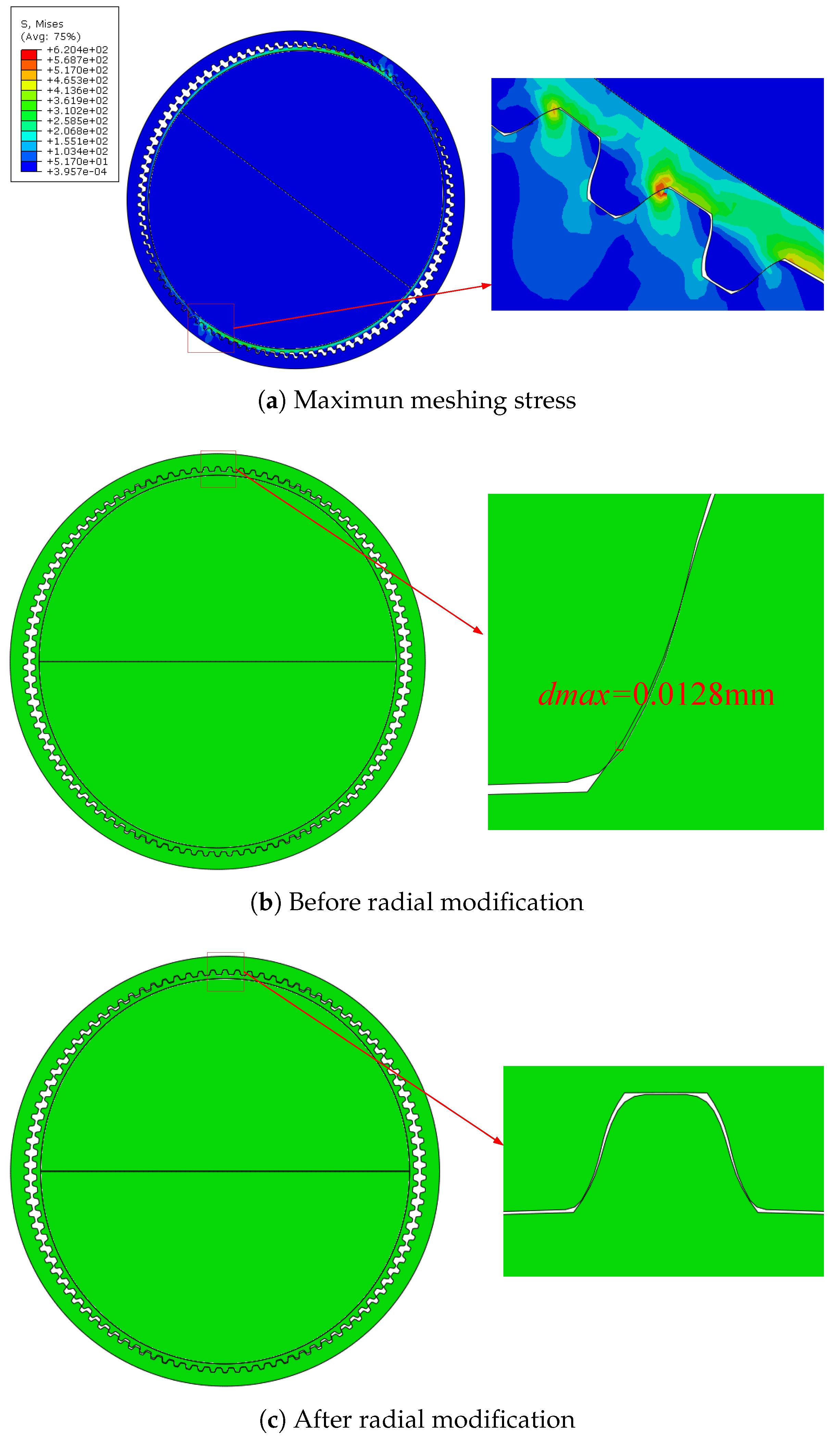
3.2. Radial Modification Method for Flexspline Tooth Profile

In practice, the teeth of the flexspline also deform after the wave generator is installed, especially at the root of the flexspline teeth, which is more pronounced. This causes interference between the flexspline tooth roots and the circular spline tooth tips, as shown in Figure 8a.

Figure 8. Radial modification diagram of flexspline tooth profile.

To determine the maximum interference, a two-dimensional finite element model of the harmonic drive is established, and after calculation, the distances from all nodes at the interference points of the circular spline tooth tips to the flexspline tooth profile in the X-axis direction are extracted, denoted as $d_1,d_2,\dots ,d_i$, where $i=1,\dots ,k$, and k is the number of nodes at the interference area of the circular spline tooth tips. The maximum interference is then given by the following:

$$d_{\max }=max\{d_1,d_2,\dots ,d_k\}.$$

(31)

Next, the tooth profiles on both sides of the flexspline are moved inward by the distance $d_{max}$ in the X-axis direction, as shown in Figure 8b. After the radial modification, the flexspline tooth roots no longer interfere with the circular spline tooth tips in the plane.

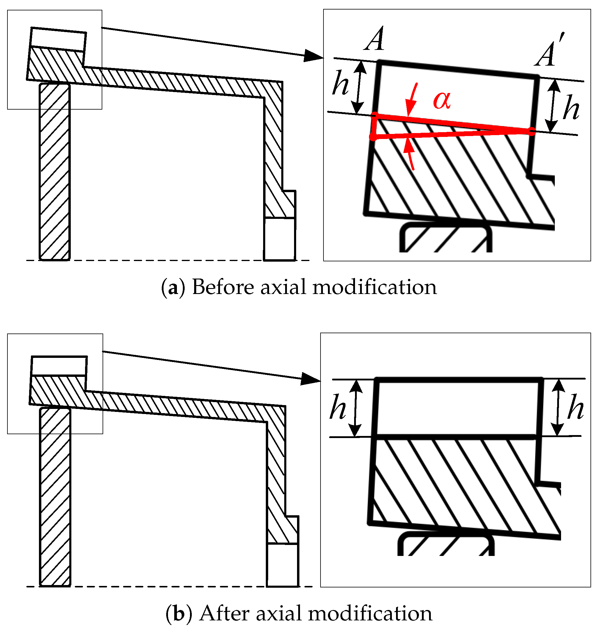
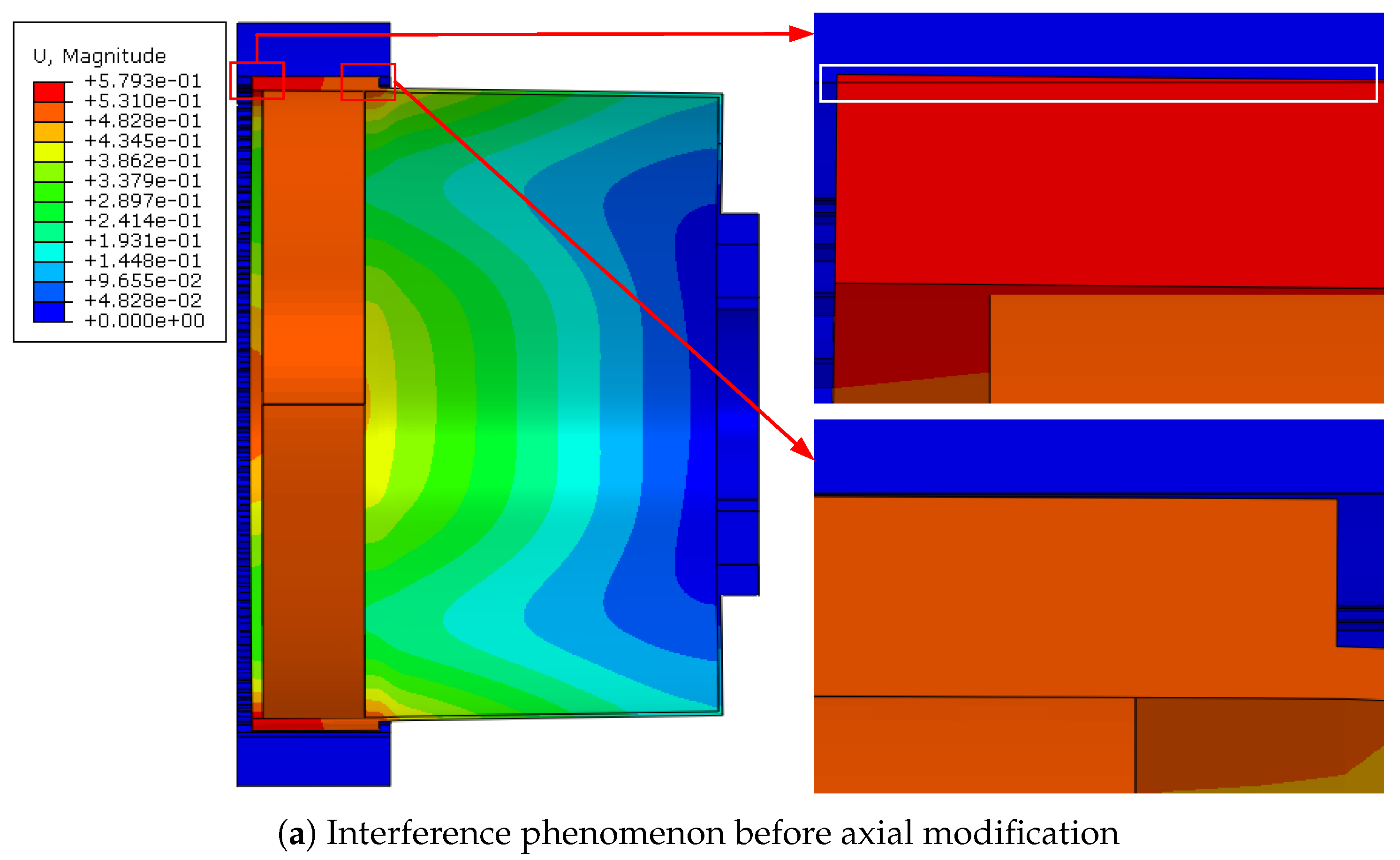
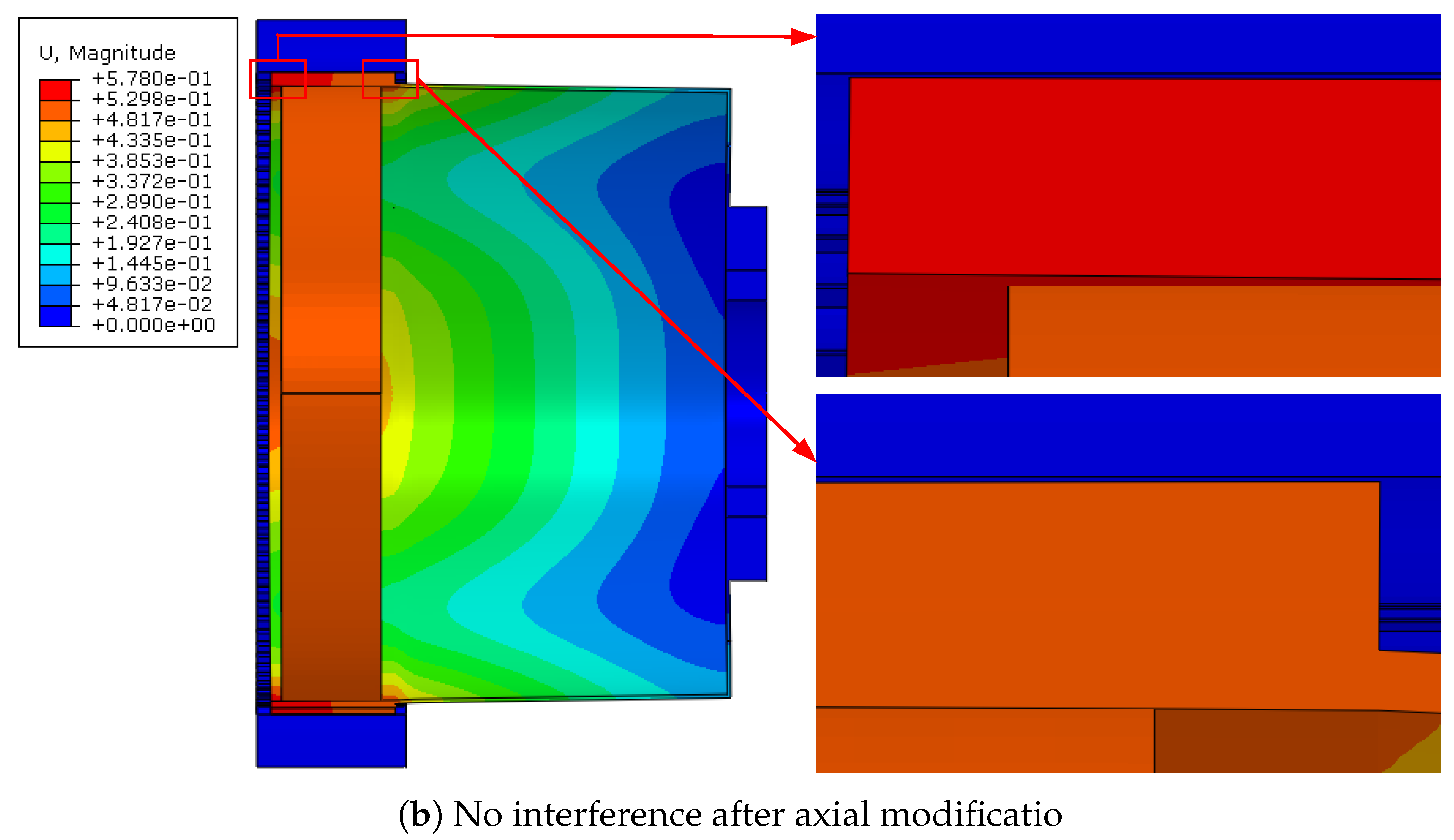
3.3. Axial Modification Method for Flexspline

In practice, one side of the flexspline typically has a cup, and after the wave generator is installed, the axial deformation of the flexspline is inconsistent, as shown in Figure 9a. The end of the flexspline furthest from the cup deviates upwards from the standard position, causing interference between the flexspline tooth tips and the circular spline tooth roots. Therefore, it is necessary to modify the flexspline axially.

Figure 9. Radial modification diagram of flexspline tooth profile.

To obtain the axial deformation of the flexspline, a three-dimensional finite element model of the harmonic drive is established. After calculation, the Y-axis coordinate values of nodes A and $A^{\prime }$ on the flexspline are obtained, as well as the axial tilt angle $\alpha$. Then, part of the tooth ring wall thickness is linearly removed, as shown by the red triangle in Figure 9a. The removal amount is zero at the end near the cup and equal to the difference in Y-axis coordinate values of A and $A^{\prime }$ at the end far from the cup. After axial modification, the flexspline tooth parts remain unchanged, and there is no interference between the flexspline tooth tips and the circular spline tooth roots, as shown in Figure 9b.

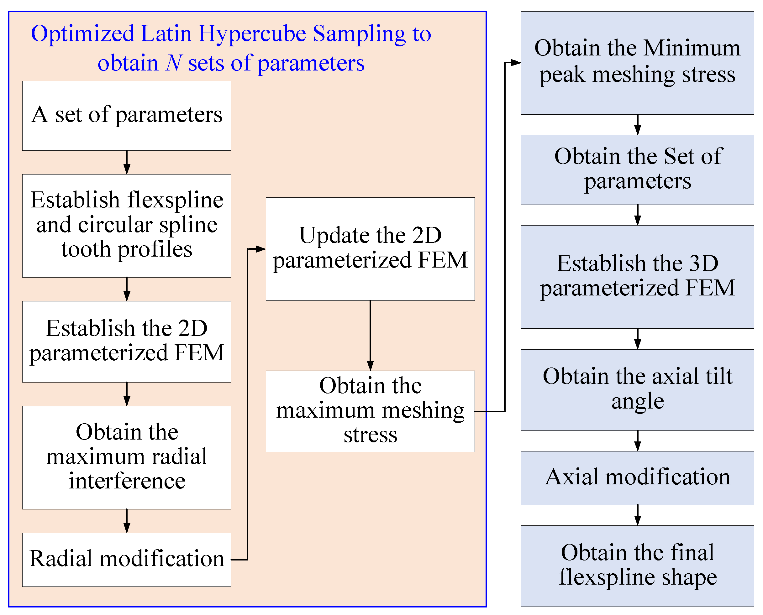
3.4. Rapid Optimization Method for Flexspline Tooth

When designing a harmonic drive, after determining the transmission ratio and module, it is necessary to determine the flexspline tooth profile. As shown in Figure 2, there are eight parameters that determine the flexspline tooth profile: $r_1$, $c_1$, $e_1$, $r_2$, $c_2$, $e_2$, $h_a$ and $h_f$. Due to the numerous parameters of the flexspline tooth profile and the time-consuming nature of finite element dynamic simulations, it is challenging to directly optimize the flexspline tooth profile parameters. Therefore, based on the parameterization method of the flexspline tooth profile, the optimized Latin hypercube sampling method, the parameterized two-dimensional finite element model, and the three-dimensional finite element model of the harmonic drive, we propose a new rapid optimization method for the flexspline tooth profile. The flowchart of this method is shown in Figure 10.

Figure 10. A new rapid optimization method for the flexspline tooth profile.

First, the optimized Latin hypercube sampling method [27] is used to sample N sets of the eight parameters of the flexspline tooth profile. Based on the parameters of each set, the corresponding flexspline and circular spline tooth profiles are established, and then the parameterized two-dimensional finite element model of the harmonic drive is created. The maximum interference between the flexspline and the circular spline in the plane is calculated and obtained, and the flexspline tooth profile is modified radially. The modified two-dimensional finite element model of the harmonic drive is then calculated, and the maximum stress during the meshing process between the flexspline and the circular spline is obtained. The set of parameters with the minimum peak stress among the N sets is selected, and based on the set of parameters, the three-dimensional finite element model of the harmonic drive is established. The axial tilt angle of the flexspline is calculated and obtained, and the flexspline is modified axially to obtain its final shape. The set of parameters is considered the optimal parameters for the flexspline tooth profile. The optimization of this paper can be represented as follows:

• Objective Function: min maximum meshing stress.
• Constraints: $r_1$, $c_1$, $e_1$, $r_2$, $c_2$, $e_2$, $h_a$ and $h_f$ in corresponding ranges.
• Design variables: $r_1$, $c_1$, $e_1$, $r_2$, $c_2$, $e_2$, $h_a$ and $h_f$.

3.5. Numerical Example

A numerical example is provided here to verify the effectiveness of the proposed method. The flexspline module is set to $m=0.5$ mm, and the transmission ratio is $i=50$. The number of teeth on the flexspline is $z_f=100$, and the number of teeth on the circular spline is $z_c=102$. The parameters of the flexspline tooth profile and their value ranges are shown in Table 1.

Table 1. The parameters of the flexspline tooth profile and their value ranges.

Parameters	Value Ranges (mm)
$r_1$	[0.650, 0.700]
$c_1$	[0.330, 0.332]
$e_1$	[0.150, 0.160]
$r_2$	[0.770, 0.820]
$c_2$	[0.329, 0.331]
$e_2$	[0.130, 0.140]
$h_a$	[0.250, 0.300]
$h_f$	[0.350, 0.400]

The ring wall thickness is given by $s={\mu }_{s}m{z}_f$, and the wall thickness of the flexspline cup is $t={\mu }_{t}s$, where ${\mu }_s$ and ${\mu }_t$ are the coefficients for the ring wall thickness and the flexspline cup wall thickness, respectively. Here, the values are set to ${\mu }_s=0.01$ and ${\mu }_t=0.6$. The resistive torque of $M=10$ Nm is applied to the flexspline, and the wave generator speed is 1500 r/min. The flexspline is assumed to possess the following properties: Young’s modulus = 200 GPa, Poisson’s ratio = 0.29, and yield strength = 860 GPa. The circular spline and wave generator are assumed to possess the following properties: Young’s modulus = 200 GPa, Poisson’s ratio = 0.29, and yield strength = 835 MPa. In this study, a parameterized model of the harmonic drive is developed using Python language, and the corresponding code is imported into Abaqus to automate the entire analysis workflow, significantly improving design efficiency. Moreover, to ensure the accuracy of the simulation, a mesh independence study is conducted, confirming that the mesh size has no significant effect on the simulation results.

The more sampling groups there are, the better the results obtained. But considering the computational load, the optimized Latin hypercube sampling number is set to $N=100$. These 100 sets of parameters are sequentially input into the established two-dimensional parameterized model of the harmonic drive for calculation. The calculations were performed on a computer with an Intel Core i7-1200 CPU, comprising 12 cores, with a total computation time of 83.3 h, averaging 50 min per set. The maximum meshing stress for the 100 sets obtained from the calculations is shown in Appendix A, with the minimum value being 620.4 MPa, as shown in Figure 11a. The maximum radial interference $d_{max}=0.0128$ mm between the flexspline and the circular spline before radial modification is shown in Figure 11b, and the result after radial modification is shown in Figure 11c.

Figure 11. Optimal parameter set radial calculation and modification results.

The optimal parameters of the flexspline tooth profile obtained from the calculations are shown in Table 2.

Table 2. The optimal parameters of the flexspline tooth profile.

Parameters	Values (mm)
$r_1$	0.68517449
$c_1$	0.33183981
$e_1$	0.15535155
$r_2$	0.78482551
$c_2$	0.13439061
$e_2$	0.32994565
$h_a$	0.29316387
$h_f$	0.35425825

Based on the parameters in Table 2, a three-dimensional finite element model of the harmonic drive was established. The simulation results show that the flexspline tooth tips at the end farthest from the cup interfere with the circular spline tooth roots, as shown in Figure 12a. The axial tilt angle was calculated to be $\alpha =0.408°$. According to the axial modification method for the flexspline described in Section 3.3, the flexspline was modified axially. After modification, there was no interference between the flexspline tooth tips and the circular spline tooth roots, as shown in Figure 12b. The final flexspline has no interference in both the radial and axial directions, and the optimal parameters for the flexspline tooth profile were obtained.

Figure 12. Radial modification diagram of flexspline tooth profile.

Based on the above calculations, under the conditions of a flexpline module $m=0.5$ mm, the number of teeth on the flexspline is $z_f=100$, and the number of teeth on the circular spline is $z_c=102$, a radial modification of 0.0128 mm and an axial modification angle of $0.408°$ were applied. As a result, a flexspline tooth profile for the harmonic drive without interference was successfully obtained.

4. Conclusions

This study proposes a novel design method for the double-circular-arc flexspline tooth profile with a common tangent, specifically tailored for harmonic drive applications. The mathematical formulations of the tooth profile curves for both the flexspline and the circular spline are derived, providing a solid theoretical foundation for geometric modeling.

Based on a parameterized two-dimensional finite element model of the harmonic drive, an optimized Latin hypercube design is employed to efficiently determine the key tooth profile parameters of the flexspline. Radial and axial profile modifications are also incorporated. Considering computational efficiency, 100 sample points are evaluated. The results show the following:

• A minimum value of maximum meshing stress of 620.4 MPa.
• A maximum radial interference of 0.0128 mm.
• An axial tilt angle of $0.408°$.

These outcomes lead to the identification of optimal tooth profile parameters and the generation of the final 3D geometry of the flexspline. The proposed method can be implemented using Python and integrated into the Abaqus platform, enabling the automation of the entire analysis process and significantly improving design efficiency, thus making it well-suited for rapid engineering development. As the performance of harmonic drives is influenced by additional design parameters, future work will incorporate these factors into the proposed parametric modeling framework to further enhance optimization and design capabilities.

References

- Musser, C.W. Strain Wave Gearing. U.S. Patent No. 2906143, 29 September 1959. [Google Scholar]
- Ivanov, M.N. The Harmonic Drive; Defense Industry Press: Beijing, China, 1987. [Google Scholar]
- Shen, Y.; Ye, Q. Theory and Design of Harmonic Drive; China Machine Press: Beijing, China, 1985. [Google Scholar]
- Raviola, A.; Martin, A.D.; Guida, R.; Jacazio, G.; Mauro, S.; Sorli, M. Harmonic drive gear failures in industrial robots applications: An overview. In Proceedings of the PHM Society European Conference, Virtual, 28 June–2 July 2021; Volume 6, p. 11. [Google Scholar]
- Yang, D.; Qiang, D.; Chen, Z.; Wang, H.; Zhou, Z.; Zhang, X. Dynamic modeling and digital twin of a harmonic drive based collaborative robot joint. In Proceedings of the 2022 International Conference on Robotics and Au-Tomation, Philadelphia, PA, USA, 23–27 May 2022; IEEE: Piscataway, NJ, USA, 2022; pp. 4862–4868. [Google Scholar]
- Pham, A.D.; Ahn, H.J. High precision reducers for industrial robots driving 4th industrial revolution: State of arts, analysis, design, per-formance evaluation and perspective. Int. J. Precis. Eng. Manuf.-Green Technol. 2018, 5, 519–533. [Google Scholar] [CrossRef]
- Fusaro, R.L. Preventing spacecraft failures due to tribological problems. In Proceedings of the 2001 Annual Meeting, No. NASA/TM-2001-210806, Orlando, FL, USA, 20–24 May 2001. [Google Scholar]
- Yang, W.; Duan, C.; Qiu, J.; Sun, J. Analysis on transient stress state of elastic thin-wall component of harmonic gear drive. Int. J. Precis. Eng. Manuf.-Green Technol. 2011, 317, 281–286. [Google Scholar] [CrossRef]
- Dong, H.; Ting, K.L.; Wang, D. Kinematic fundamentals of planar harmonic drives. ASME J. Mech. Des. 2011, 133, 011007. [Google Scholar] [CrossRef]
- Kondo, K.; Takada, J. Study on tooth profiles of the harmonic drive. ASME J. Mech. Des. 1990, 112, 131–137. [Google Scholar] [CrossRef]
- Chen, X.; Liu, Y.; Xing, J.; Lin, S.; Xu, W. The parametric design of double-circular-arc tooth profile and its influence on the function-al backlash of harmonic drive. Mech. Mach. Theory 2014, 73, 1–24. [Google Scholar] [CrossRef]
- Yao, Y.P.; Chen, X.X.; Xing, J.Z. Complex cycloidal tooth profile of circular spline in harmonic drive and its optimal fitting research. J. Ind. Prod. Eng. 2017, 34, 1–8. [Google Scholar] [CrossRef]
- Shi, W.; Zhen, J.; Niu, T.; Song, H. A New Type of Cycloidal Tooth Profile Design and Analysis of Harmonic Gear Drive. Mech. Eng. Technol. 2018, 7, 43–53. [Google Scholar] [CrossRef]
- Ji, C.; Zhang, Z.; Cheng, G.; Kong, M.; Li, R. Design, modeling, and control of a compact and reconfigurable variable stiffness actuator using disc spring. J. Mech. Robot. 2024, 16, 091006. [Google Scholar] [CrossRef]
- Kosse, V. Analytical investigation of the change in phase angle between the wave generator and the teeth meshing zone in high-torque mechanical harmonic drives. Mech. Mach. Theory 1997, 32, 533–538. [Google Scholar] [CrossRef]
- Zhang, L.; Yang, W.; Jiang, Q.; Wang, C.; Huang, W. Structural stress analysis of the core component of harmonic reducer. J. Mech. Transm. 2018, 42, 114–117. [Google Scholar]
- Gravagno, F.; Mucino, V.H.; Pennestri, E. Influence of wave generator profile on the pure kinematic error and centrodes of harmonic drive. Mech. Mach. Theory 2016, 104. [Google Scholar] [CrossRef]
- Sahoo, V.; Maiti, R. Load sharing by tooth pairs in involute toothed harmonic drive with conventional wave generator cam. Meccanica 2017, 53, 373–394. [Google Scholar] [CrossRef]
- Li, X.; Song, C.; Yang, Y. Optimal design of wave generator profile for harmonic gear drive using support function. Mech. Mach. Theory 2020, 152, 103941. [Google Scholar] [CrossRef]
- Rheaume, F.E.; Champliaud, H.; Liu, Z. Understanding and mod-elling the torsional stiffness of harmonic drives through finite-element method. Proc. Inst. Mech. Eng. Part C J. Mech. Eng. Sci. 2009, 223, 515–524. [Google Scholar] [CrossRef]
- Song, C.; Li, X.; Yang, Y.; Sun, J. Parameter design of double-circular-arc tooth profile and its influence on meshing characteris-tics of harmonic drive. Mech. Eng. Technol. 2022, 167, 104567. [Google Scholar]
- Pacana, J.; Siwiec, D.; Pacana, A. Numerical analysis of the kine-matic accuracy of the hermetic harmonic drive in space vehicles. Appl. Sci. 2022, 13, 1694. [Google Scholar] [CrossRef]
- Song, C.; Zhu, F.; Li, X.; Du, X. Three-dimensional conjugate tooth surface design and contact analysis of harmonic drive with dou-ble-circular-arc tooth profile. Chin. J. Mech. Eng. 2022, 36, 83. [Google Scholar] [CrossRef]
- Cheng, Y.; Chen, Y. Design, analysis, and optimization of a strain wave gear with a novel tooth profile. Mech. Mach. Theory 2022, 175, 104953. [Google Scholar] [CrossRef]
- Kayabasi, O.; Erzincanli, F. Shape optimization of tooth profile of a flexspline for a harmonic drive by finite element modelling. Mater. Des. 2007, 28, 441–447. [Google Scholar] [CrossRef]
- Leon, D.; Arzola, N.; Tovar, A. Statistical analysis of the influence of tooth geometry in the performance of a harmonic drive. J. Braz. Soc. Mech. Sci. Eng. 2015, 37, 723–735. [Google Scholar] [CrossRef]
- Rajabi, M.M.; Ashtiani, B.A.; Janssen, H. Efficiency enhancement of optimized latin hypercube sampling strategies: Application to monte carlo uncertainty analysis and meta-modeling. Adv. Water Resour. 2015, 76, 127–139. [Google Scholar] [CrossRef]
Disclaimer/Publisher’s Note: The statements, opinions and data contained in all publications are solely those of the individual author(s) and contributor(s) and not of MDPI and/or the editor(s). MDPI and/or the editor(s) disclaim responsibility for any injury to people or property resulting from any ideas, methods, instructions or products referred to in the content. |
© 2025 by the authors. Licensee MDPI, Basel, Switzerland. This article is an open access article distributed under the terms and conditions of the Creative Commons Attribution (CC BY) license (https://creativecommons.org/licenses/by/4.0/).