Abstract
This research article tackles the control problem of an inverted pendulum, also known as the Furuta pendulum, mounted on a velocity-controlled robot manipulator in two configurations: the rotary pendulum and the translational pendulum. Differently from most of the existing control architectures where the motor actuating the pendulum motion is torque-controlled, the proposed control architecture exploits the inner velocity loop usually available on industrial robots, thus easing the implementation of an inverted pendulum. Another aspect investigated in this paper and mostly overlooked in the literature is the digital implementation of the control and, specifically, the latency introduced by the digital controller. The proposed control solution explicitly models such effects in the control design phase, improving the closed-loop performance. The additional novelty introduced by this paper is the friction compensation that is essential in the swing-up phase of the inverted pendulum, whereas classical control strategies for the nonlinear swing-up usually neglect this effect, and their solutions lead to control failures in practical systems. This paper presents detailed modeling and experimental identification phases followed by the control design of both the nonlinear swing-up algorithm and the linear stabilization controller, both experimentally validated on a Meca500 robotic arm controlled via an EtherCAT communication protocol by a mini PC featuring a Xenomai real-time operating system. The overall system showcases the potential of high-performance digital control systems in industrial robotic applications.
1. Introduction
The control of nonlinear and underactuated mechanical systems is a topic of great interest in control engineering, with numerous applications in robotics, industrial automation, and autonomous vehicles. Among these systems, the inverted pendulum, also known as the Furuta pendulum, in both its rotary and translational versions, serves as an ideal test bench for developing and validating new control strategies, and it has been exploited in control education for many years, since the seminal paper [1] until the most recent one [2]. The rotary pendulum consists of a horizontal arm mounted on a rotary axis controlled by an actuator (usually an electric motor) and a pendulum that is free to oscillate on a vertical plane perpendicular to the arm. In the translational version, the suspension point of the pendulum can translate along a fixed direction actuated by a motor.
In both cases, the vertical position of the pendulum is an unstable equilibrium, and the main challenge is to design control strategies that allow the pendulum to reach this position and keep it stable. The control of the inverted pendulum can be divided into two main problems. The first is the swing-up, which involves raising the pendulum from its initial position, typically hanging down, to the vertical position. The second problem is balancing and stabilization: once the pendulum reaches the vertical position, the control system must prevent it from falling by stabilizing the position and compensating for disturbances. Several practical applications can benefit from an effective and reliable solution of this control problem, from transport machines, including drones [3], to structure construction [4] and people transportation [5].
The complexity of the problem arises from several factors. First, there is the issue of under-actuation, as the torque applied to the pendulum is zero. In addition, the nonlinear dynamics of the system, described by equations of motion that include nonlinear terms and the coupling between state variables, add further difficulty to the control. Finally, real-world effects in digital control, such as friction, sampling delay and latencies, signal quantization, measurement noise, and actuator dynamics, can degrade control performance, making pendulum control even more challenging.
1.1. Related Works
Numerous control strategies have been developed for the inverted pendulum; a good survey is [6]. The following subsections discuss not only those proposed to solve the two subproblems, stabilization and swing-up, but also the existing contributions and their limitations in tackling the additional problems listed so far, i.e., digital implementation of the control law, latencies in the control architecture, static friction, and actuator dynamics.
1.1.1. Stabilization Control
Several approaches have been developed to solve the stabilization problem. The LQR (Linear Quadratic Regulator) controller is widely used to stabilize the system by minimizing a cost function that penalizes deviations from the equilibrium state and control effort [7]. Even more recent robust control strategies have been applied to the pendulum stabilization, e.g., via Linear Matrix Inequalities [8]. Classical PID (Proportional-Integral-Derivative) controllers can be applied, but they are generally less effective than optimal control methods. Model predictive control (MPC), predicting the future trajectory of the system and optimizing the control input based on physical and actuator constraints, can also be used [9]; MPC is particularly useful when dealing with system delays and when limited control effort is available; however, the nonlinear nature of the system requires nonlinear MPC that can be computationally demanding and not suitable for small sampling times. Nonlinear control algorithms, based on Lyapunov-based approaches, can also stabilize the pendulum to the upright position, yielding a larger size estimation of the domain of attraction than the one obtained with the traditional linear approach [10], or can stabilize the pendulum and track a reference trajectory with the arm at the same time, e.g., [11,12]. However, they are all generally more sensitive to parametric uncertainties and neglect the limitations introduced by the digital control implementation.
1.1.2. Swing-Up Strategies
Various strategies have been developed to move the pendulum from its initial position to the vertical one. Energy-based control is the most popular way; this method calculates the energy required to reach the upright position and gradually injects it into the system [13,14]. A similar method injecting energy into the system is the exponentiation of the pendulum [9], such that the amount of supplied energy is minimal as long as the pendulum is relatively near the upright position. The advantage is the reduced control effort; however, the system may take a long time to reach the equilibrium. However, heuristic solutions are adopted to “solve practical problems”, as in [13], mostly related to non-ideal actuation and friction. Therefore, aggressive, robust sliding mode controllers have been designed to swing the pendulum up even in the presence of friction and uncertain parameters [15]. Also, soft-computing techniques have been proposed to obtain a less sensitive system to inaccurate state measurements and parametric uncertainties, such as fuzzy logic controllers [16,17]. Nevertheless, in all cited cases, the control input was the actuator torque or voltage, which can be difficult if the pendulum is actuated by the motion of a velocity-controlled robot or joint.
1.1.3. Effects of Sampling Delay
With the adoption of digital controllers, the issue of sampling delay arises. This delay can significantly impact control performance, particularly in systems with fast dynamics, such as the Furuta pendulum with short-length arms. Studies have shown that sampling delay can compromise the system’s stability, especially when dealing with short pendulums that exhibit rapid motion. Furthermore, direct angular velocity measurement is not always possible in the presence of delays, making it necessary to estimate this quantity from angle values acquired in discrete time. A crucial result demonstrated in recent research is the existence of a critical sampling time beyond which linear stabilization of the pendulum becomes impossible [7,18]. More critical situations may arise when delay is stochastic such as in stochastic switched systems [19]. However, in this paper all delays are considered deterministic owing to the adoption of a real-time operating system. In fact, we selected an open-source real-time digital control architecture in which we implemented a novel control algorithm that explicitly takes into account the unavoidable latencies and the finite bandwidth of the servo actuating the pendulum motion.
1.2. Research Objectives and Contribution
It is important to clarify that the aim of this paper is not the proposition of a new control method that overcomes the performance of control solutions devised so far for the inverted pendulum. Rather, the objective of this work is to design standard stabilization and swing-up controllers of a Furuta pendulum, but by exploiting a dynamic model that considers both the mechanical dynamics of the pendulum, including the friction, and the closed-loop dynamics of a velocity-controlled robot, including the effects of digital control and control architecture latency. The research results will show that the control performance is negatively affected if all these dynamics are neglected.
A fundamental difference between this work and the existing state of the art is the choice of control strategy. In most conventional approaches, control is applied in terms of actuator torque or voltage, assuming direct control over the system’s dynamic response. However, in this work, we adopt a velocity-based control approach, where commands are sent directly as velocity references to the robot joints. This methodology aligns better with the natural actuation capabilities of industrial robots, simplifies the controller implementation, and allows for precise real-time execution. By departing from torque control and leveraging velocity commands, this approach offers a novel and practical alternative that can be effectively implemented on industrial robotic platforms.
To ensure precise control performance, a Linear Quadratic Gaussian (LQG) controller was designed and implemented, explicitly considering the dynamics of the velocity-controlled robot joints and the system latency. A key aspect of this research was an experimental model identification procedure to characterize the relationship between the desired velocity commands and the actual executed velocities of the robot. This identification process allowed for an accurate determination of the system’s dead time, which is an intrinsic part of the robot’s digital control interface and must be accounted for in the control design. Unlike classical approaches that assume an ideal actuation response, this study directly incorporates real-world effects, such as actuation delays, into the control model.
To push the performance limits of the system, the entire control architecture has been implemented with a sampling period of 1 ms, leveraging the Xenomai real-time framework. This choice enables hard real-time execution, ensuring precise timing and reducing jitter in control execution. The use of EtherCAT as the communication protocol further enhances the system’s responsiveness by providing fast and deterministic data exchange between the controller and the robot. Given that the available robot, a Meca500 by Mecademic, can be commanded at a maximum sampling rate of 1 kHz, this implementation fully exploits the available hardware capabilities, minimizing control delays as much as possible.
The combination of velocity-based control, LQG control, real-time execution, and actuator-aware modeling represents a novel strategy for achieving stable inverted pendulum behavior on a robotic platform. This work demonstrates how a high-performance digital control system can be designed while considering real-world constraints such as sampling delay, communication latency, and actuator dynamics.
2. Materials and Methods
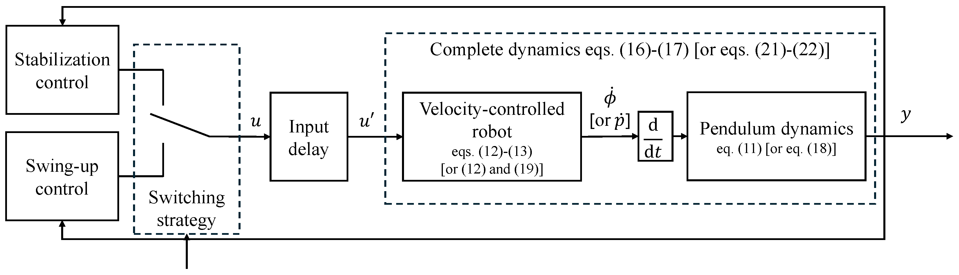
This section is devoted to presenting the materials and methods used in this research. The experimental setup is described in Section 2.1 in terms of both hardware and software components. The main contribution is the adoption of the Xenomai real-time operating framework [20] within a ROS2 network. The literature reports various benchmarks of robotics middleware frameworks, such as ROS2 and OROCOS [21], but only over PREEMPT_RT and vanilla Linux kernels since there is no ROS2 support yet for Xenomai, while only ROS implementations can be found in the related literature, such as [22]. Section 2.2 reports the dynamic modelling process of both rotary and translational pendulums, with a significant novelty compared to the classical dynamic models of the inverted pendulum used in the literature, where most of the approaches consider a torque-controlled motor to actuate the pendulum motion. Instead, a velocity-controlled robot is used here, with the considerable advantage of allowing the adoption of more widely available hardware and devolving the computation of the control torque to a lower-level controller that has to reject unmodeled dynamics and external disturbances, so that the design of the pendulum controller is easier. On the other hand, velocity control interfaces are usually characterized by significant latency or dead time; therefore, the stabilization control of the pendulum has to properly take them into account. Section 2.4 is devoted to describing the whole control system of both rotary and translational pendulums, which includes two control actions, one for the stabilization of the pendulum around the unstable position and one for the swing-up; a suitable switching strategy is also proposed to decide which control action should be active in each time instant of the system operation. The main novelties of the first control law consist in the consideration of the velocity loop dynamics including the input delay, while the swing-up control strategy explicitly takes into account the presence of friction on the pendulum axis, which is usually neglected in the literature.
2.1. Experimental Setup
The two versions of the inverted pendulum considered in this work are moved by employing the Meca500 robot by Mecademic. The hardware/software architecture is shown in Figure 1. The Meca500 robot accepts velocity commands through an EtherCAT interface at 1 kHz. The pendulum is mechanically connected to the robot flange through a bearing. An incremental encoder measures the pendulum angle. An Arduino microcontroller converts the encoder signals to the actual angle and sends it to the control PC via a serial interface. The control PC hosts a ROS2 network with three primary nodes: the Encoder ROS Driver reads the encoder angle from the serial interface and republishes it on the ROS2 network; the Meca500 Driver communicates via the EtherCAT protocol with the robot, and it publishes the robot state and reads the joint velocity command from the ROS2 network; the pendulum controller implements the control algorithms described in the following sections and publishes the joint velocity commands on the appropriate ROS topic. To meet the strict control cycle deadline, we adopt the Xenomai real-time framework in all the described ROS2 nodes to run the algorithms in dedicated real-time threads.
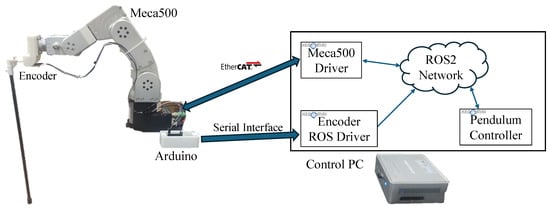
Figure 1.
Hardware/software architecture of the experimental setup.
2.2. Dynamic Modelling
The inverted pendulum in this work consists of two main components: a robotic arm moving the suspension point of a pendulum that is free to oscillate in the vertical plane. The two classical versions of the pendulum are considered. First, the rotary pendulum is actuated by moving only the first joint of the robot while all other joints are fixed such that the arm is fully stretched. Second, the translational pendulum is actuated by moving the robot tool center point in the Cartesian space along a fixed direction; this means that all the robot joints need to move in a coordinated fashion. The following subsections report the dynamic models of both cases derived using the Lagrangian approach, taking into account that the control input is the vector of robot joint velocities.
Rotary Pendulum
The rotary pendulum system is depicted in left picture of Figure 2. A rigid bar of mass m, inertia moment and center of mass at a distance from the rotation axis is attached to the Meca500 arm in a configuration such that the distance of the pendulum suspension point from the rotating axis is , and the inertia moment of the rotating arm is . The system has two degrees of freedom, which can be represented by the two generalized variables: , the angle of the rotating arm about a vertical axis, and , the angle of the pendulum about a horizontal axis, assumed to be zero when the pendulum is upright. Given a fixed reference frame with the z axis along the axis of rotation, the x axis along the rotation arm when , and the y axis to complete a right-handed frame, the Cartesian coordinates of the pendulum’s center of mass can be expressed in terms of the generalized coordinates by simple kinematic relationships [23] as
Taking time derivatives gives the velocity components of the pendulum’s center of mass
Therefore, the total kinetic energy of the system is
The total potential energy of the system is simply the gravitational energy of the pendulum center of mass, assumed to be zero when the pendulum is vertical, i.e., when , namely
where g is the gravitational acceleration magnitude.
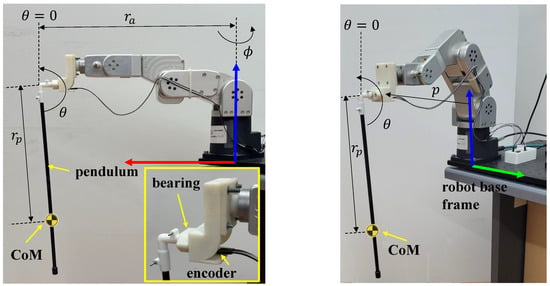
Figure 2.
Meca500 robot in the two configurations to actuate the pendulum. In the rotary one (left), the only active joint is the first one (). In the translational one (right), the tool center point is moved along the y axis of the robot base frame. Axes of the reference frame are depicted in the RGB () convention.
Given the Lagrangian function , the equations of motion can be written in the well-known form
where is the dissipative viscous friction torque acting on the pendulum, and is the dissipative viscous friction torque acting on the arm, with representing the viscous friction coefficient. Since the arm joint is velocity-controlled through the manufacturer’s low-level control board, the only equation of motion of interest is that of the pendulum angle, i.e.,
This equation clearly shows that the pendulum motion can be controlled by acting on the arm joint acceleration . However, since the joint is velocity-controlled, the actual control input is the desired velocity u given as reference to the low-level joint velocity controller. Therefore, Equation (11) has to be coupled to the closed-loop dynamics of the velocity-controlled joint. This dynamic has been experimentally identified as a linear system with 2-dimensional state space equations
where
and , with being the delay of six samples introduced by the robot firmware interface that are necessary to process each velocity command with a sampling time of ms. The adopted experimental identification procedure is a standard subspace identification run in MATLAB R2022b after acquiring an input–output (-) dataset with a constant amplitude chirp input signal in the frequency range Hz with a duration of 100 s. By combining Equations (11)–(13), the complete system is described by nonlinear dynamics with the following state variables (note that is a 2-dimensional state variable)
and equations
Note that the output vector y has a length of 4 since we assume the measurement of both the position and velocity of the robot’s and pendulum’s joints, owing to a suitable elaboration of the encoder signals. Nevertheless, in the section devoted to the control design, a Linear Quadratic Gaussian (LQG) control scheme will be adopted for the pendulum stabilization to reduce the effects of noise for small oscillations. Such a reduction will not be necessary during the swing-up phase, which involves larger oscillations with greater velocities of both joints.
2.3. Translational Pendulum
The equations of motion in this case are even simpler than those for the rotary pendulum and can be derived in a similar fashion by using the Lagrangian formalism. With reference to the right picture of Figure 2, denoting with p the translation of the pendulum suspension point along the y axis of the robot base frame, the equation of motion is [1]
As before, this equation has to be combined with the dynamics of the velocity-controlled robot. By applying a standard kinematic control [24], the robot joint velocities are suitably commanded given a desired velocity u of the pendulum suspension point and a zero linear and angular velocity along all other directions of the robot tool. According to validation experiments, the dynamics between the input desired velocity u and the actual one is the same as the one identified for the single joint closed-loop dynamics in (12) and (13); therefore, the actual robot velocity is
and the state of the nonlinear system is (again, is a 2-dimensional state)
and the whole system dynamic model can be written in the form
where the control input (with as the usual input delay of the control interface) is the desired tool velocity along the y axis of the base frame. Note that the velocity can be related to the measured robot joint velocities through the well-known robot Jacobian matrix . In detail, since the robot has to move the tool along the y axis only while keeping its orientation fixed, the desired tool twist v, defined as the stack of the linear and angular 3-dimensional velocity vectors with respect to the base frame, has the second component (along the y axis) equal to and the other five components equal to zero, i.e., . It is well known that the 6-dimensional end-effector twist v is related to the joint velocity as [25]; hence, by inverting this relationship, it is possible to command the joint velocities given the desired tool velocity v.
2.4. Control Design
Even though the related literature reports a few control solutions that solve both the swing-up and the stabilization control using the same control strategy, e.g., those based on model predictive control [26], the classical approach of different strategies for stabilization and swing-up is adopted here in view of the limited computational capacity of the available hardware and the small sampling time targeted for the application, which is necessary to have a closed-loop system with a fast reaction time to external disturbances. The whole control system is sketched in the block scheme of Figure 3, where the three blocks from u to y highlight the novelty of the proposed dynamic model that takes into account input delay and actuation dynamics as well as mechanical dynamics.
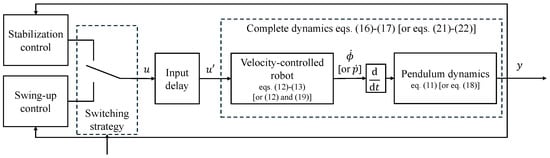
Figure 3.
Block scheme of the inverted pendulum control system. The blocks relating the control input u to the measured output y model the input delay, the dynamics of the velocity-controlled robot, and the mechanical dynamics (equation numbers in square brackets refer to the translational pendulum; the others refer to the rotary pendulum).
2.4.1. Stabilization Control
Since the amplitude of the oscillations around the stabilized equilibrium point is expected to be small, the classical control design method based on the system linearized model can be adopted. The novelty here is the explicit consideration of both the actuator dynamics and the digital implementation of the control algorithm, including the input delay. The section devoted to experiments contains some tests that show how neglecting such effects significantly reduces the amplitude of the region of attraction of the stabilized equilibrium point.
The control design will be presented with reference to the rotary pendulum only, since it is the same for the translational pendulum. Linearization of Equation (16) around the equilibrium point in the origin of the state space yields the linear time-invariant system
with
where is the total inertia moment of the pendulum.
The next step to design a digital LQG controller is the discretization of the model above with the Zero-Order-Hold method at sampling time , yielding state equations in the discrete-time state , with input , and output
with the state space matrices
Finally, the input delay of six samples that relates the input to the actual input u can be modeled in the discrete time by a simple 6-dimensional buffer, which is a linear system with 6 states , and a state matrix with 6 eigenvalues in the origin, i.e.,
where denotes the actual control input, and
The resulting complete linear system is finite dimensional with states, , and state space equations
where it is worth recalling that is the desired velocity of the rotary joint, and is the vector of the measured pendulum position, pendulum velocity, rotary joint position, and rotary joint velocity. Differently from most of the models used in the literature, this model takes into account all dynamic effects, i.e., mechanical dynamics, velocity loop dynamics of the rotary joint, as well as the input delay due to the digital implementation.
The design of the stabilization control is straightforward as it is a standard LQG controller; thus, the model above is re-written in the form
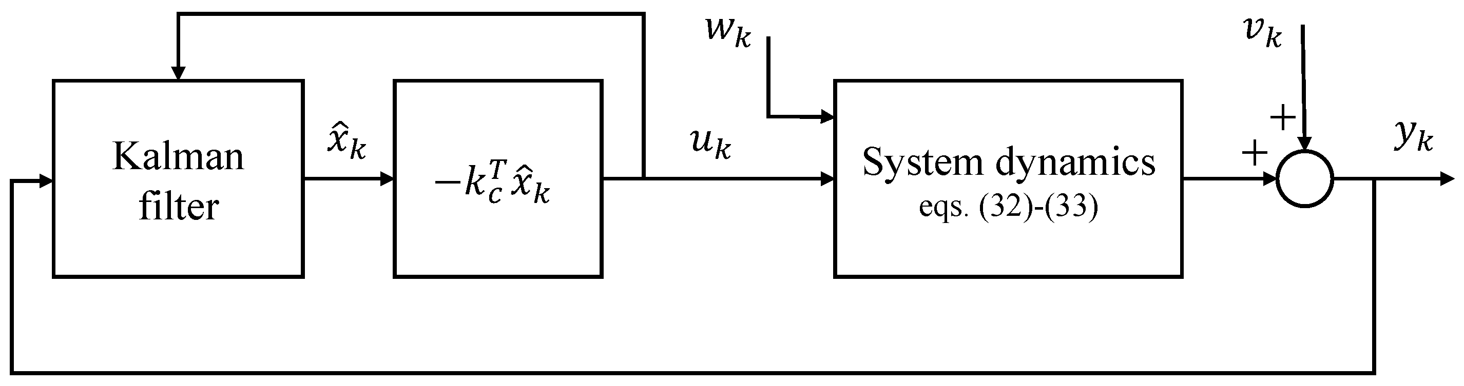
where and represent white Gaussian process and measurement noise, respectively. The control scheme is depicted in Figure 4, where the Kalman filter is used to obtain a state estimate in the presence of noise that is optimal given the noise statistics. The Kalman filter equations are not reported here for brevity but the interested reader can find them, e.g., in [27]. The second step of the design is the solution of the optimization problem that has to minimize the following cost function [28]
where Q is a positive semi-definite matrix weighting the state, and r is a positive scalar weighting the control effort. The optimal control law is
where is the optimal gain vector, and P is the solution of the algebraic Riccati equation associated with the cost function (36) and the dynamic system (32) and (33).
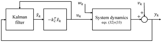
Figure 4.
Block scheme of the LQG controller to stabilize the inverted pendulum.
2.4.2. Swing-Up Control of the Rotary Pendulum
Inspired by the energy-based approach in [1], the swing-up algorithm aims at bringing the total mechanical energy of the uncontrolled pendulum to the value when the pendulum is upright. The control law will be presented for both the rotary and the translational pendulum, since they exhibit differences.
The total mechanical energy of the uncontrolled rotary pendulum
is zero when the pendulum is stationary () in the vertical position (). The control law to bring this energy to the desired value zero can be derived using a Lyapunov-like method by considering the positive definite function of the energy, which is always positive except when it is zero, which only occurs when the energy is zero,
Its time derivative along the trajectories of the system (11) is
This expression suggests the following choice of the control acceleration , given a positive gain :
which, substituted in (40), gives
which is always non-positive, except for when or . Note that the pendulum positions corresponding to are not equilibrium points; hence, the system cannot stay in such positions with . The case is an equilibrium only in the upright (unstable) and downright (stable) positions of the pendulum; therefore, to start a swing-up from the stable position, an external force has to be applied to the pendulum to let , and thus . In conclusion, the energy squared decreases and asymptotically tends to zero. Note that the energy E in (38) can be both positive and negative, and it can be zero not only when and , but also for and such that . However, implies that tends to zero, this means that if there exists a time instant such that , then , and thus the state of the pendulum sooner or later will reach the upright position with . Note also that this does not mean that the equilibrium is stable, as it actually is unstable with this control law. Therefore, a stabilization control law is needed to keep the pendulum upright as soon as it comes close to this equilibrium point.
A twofold comment on the control law (41) is in order. First, most of the energy-based control solutions neglect the friction torque acting on the pendulum; however, without the friction compensation term in (41), the swing-up is difficult as the energy might not increase enough. Nevertheless, the term is well defined only when ; therefore, a suitable regularization is needed to allow passing through the singularity. Given a small positive value , a possible solution is to compute the friction compensation term as the following function of and :
Finally, since the robot is velocity-controlled, the joint acceleration in (41) has to be integrated before being commanded to the robot.
2.4.3. Swing-Up Control of the Translational Pendulum
Since the energy of the uncontrolled pendulum is always the same as in (38), the same method as in the previous subsection can be applied also in this case. Therefore, by substituting the control law
in the pendulum dynamic Equation (18), the time derivative of the function becomes
The same conclusion as in the rotary pendulum case can be drawn on the effect of the swing-up control law (44), and also a regularization similar to (43) is needed as the friction compensation term, i.e.,
Again, the control acceleration has to be integrated before being commanded to the robot.
2.4.4. Switching Strategy
As already discussed, the swing-up control law does not stabilize the pendulum in the upright position; therefore, the control input has to be switched from the swing-up (Equation (41) for the rotary pendulum and Equation (44) for the translational pendulum) to the stabilization (37). Of course, the stabilization controller is only a local controller and thus it might happen that the pendulum falls if a sufficiently large force is applied to the pendulum bar. Therefore, the control input has to be switched again to the swing-up strategy to bring the pendulum to the upright position again. Of course, the decision variable of the switching is the measured pendulum angle. To allow the transient dynamics of the closed-loop system with the stabilization control active die out and to avoid continuous switches between the two control modes due to small perturbations or measurement noise, the switching is implemented with a hysteresis relay, graphically represented in Figure 5.
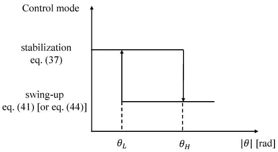
Figure 5.
The switching strategy between swing-up and stabilization controllers.
Specifically, the switching strategy is as follows:
- Stabilization Mode: When the absolute value of the pendulum angle is small, rad, the system operates in stabilization mode using the LQG controller (37) to maintain the pendulum near the upright position.
The hysteresis band ensures that the controller does not switch back and forth continuously when is close to the switching threshold due to sensor noise. The lower value is selected slightly lower than an estimate of the region of attraction of the stabilization controller. This value is experimentally identified as explained in Section 3. The higher value is selected as plus an angle experimentally tuned on the basis of the dynamic performance of the system under the stabilization controller, i.e., rad, as explained in more detail in Section 3.4. This value is five times higher than the encoder resolution, which makes the switching strategy robust to measurement noise too.
3. Experimental Results
This section presents the results of the following experiments:
- Case study 1: test of the stabilization control for both the rotary and translational pendulum designed as explained in Section 2.4.1;
- Case study 2: test of the stabilization control for both the rotary and translational pendulum designed by neglecting the robot velocity loop dynamics;
- Case study 3: test of the swing-up control for both the rotary and translational pendulum designed as explained in Section 2.4.2 and Section 2.4.3, respectively.
The dynamic parameters of the mechanical system are those reported in Table 1.

Table 1.
Dynamic parameters of the mechanical system.
3.1. Case Study 1
The first experimental test aims to find the maximum value of the threshold allowed by the designed stabilization controller. Once the controller is activated with the pendulum in the naturally stable position, the user slowly brings the pendulum towards the upright position while looking at the PC monitor where a big red circle appears as soon as the threshold is overcome (see the video abstract of this paper in Supplementary Materials); the user immediately releases the pendulum that the robot tries to keep in the vertical position.
The LQG controller presented in Section 2.4.1 for the rotary pendulum has been designed using the following weights:
The resulting vector gain is
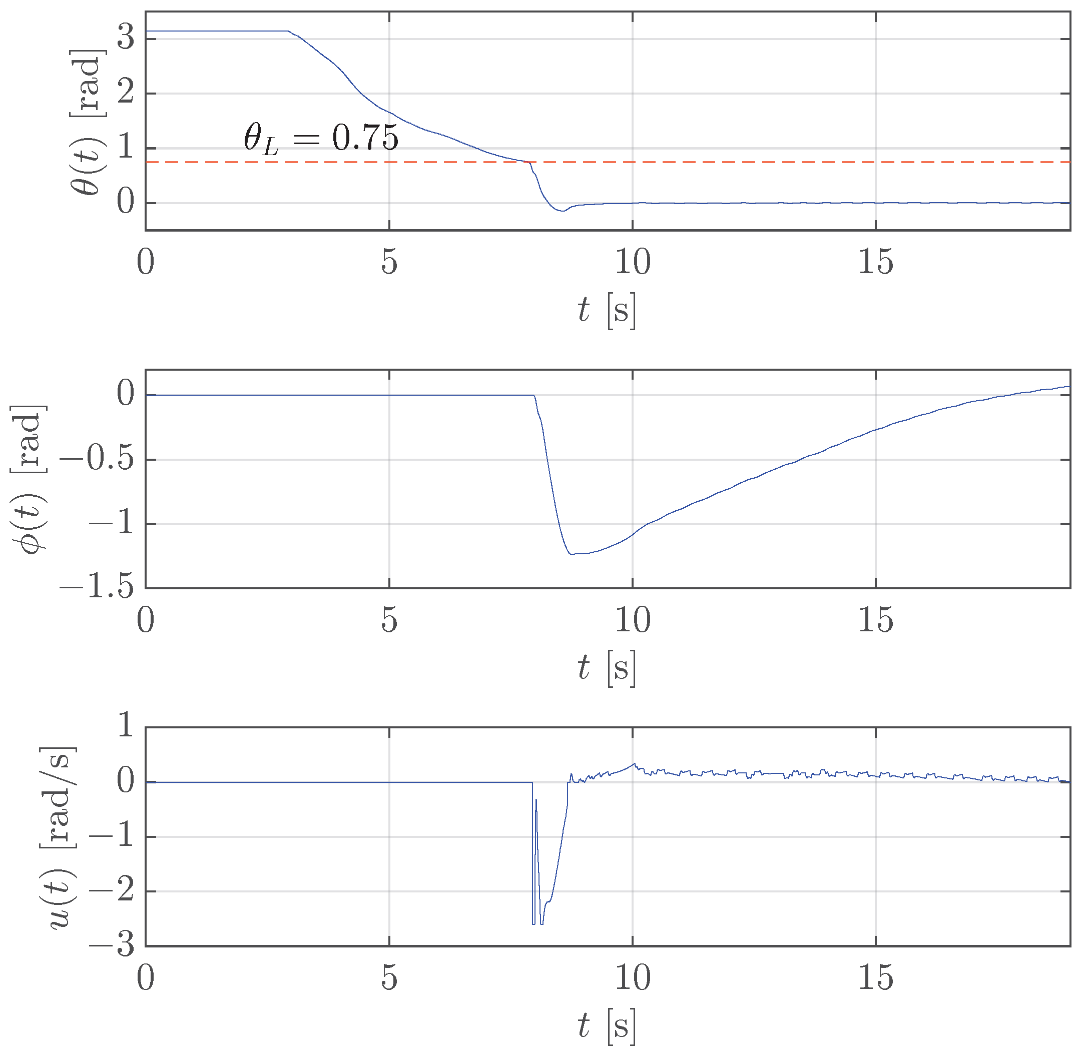
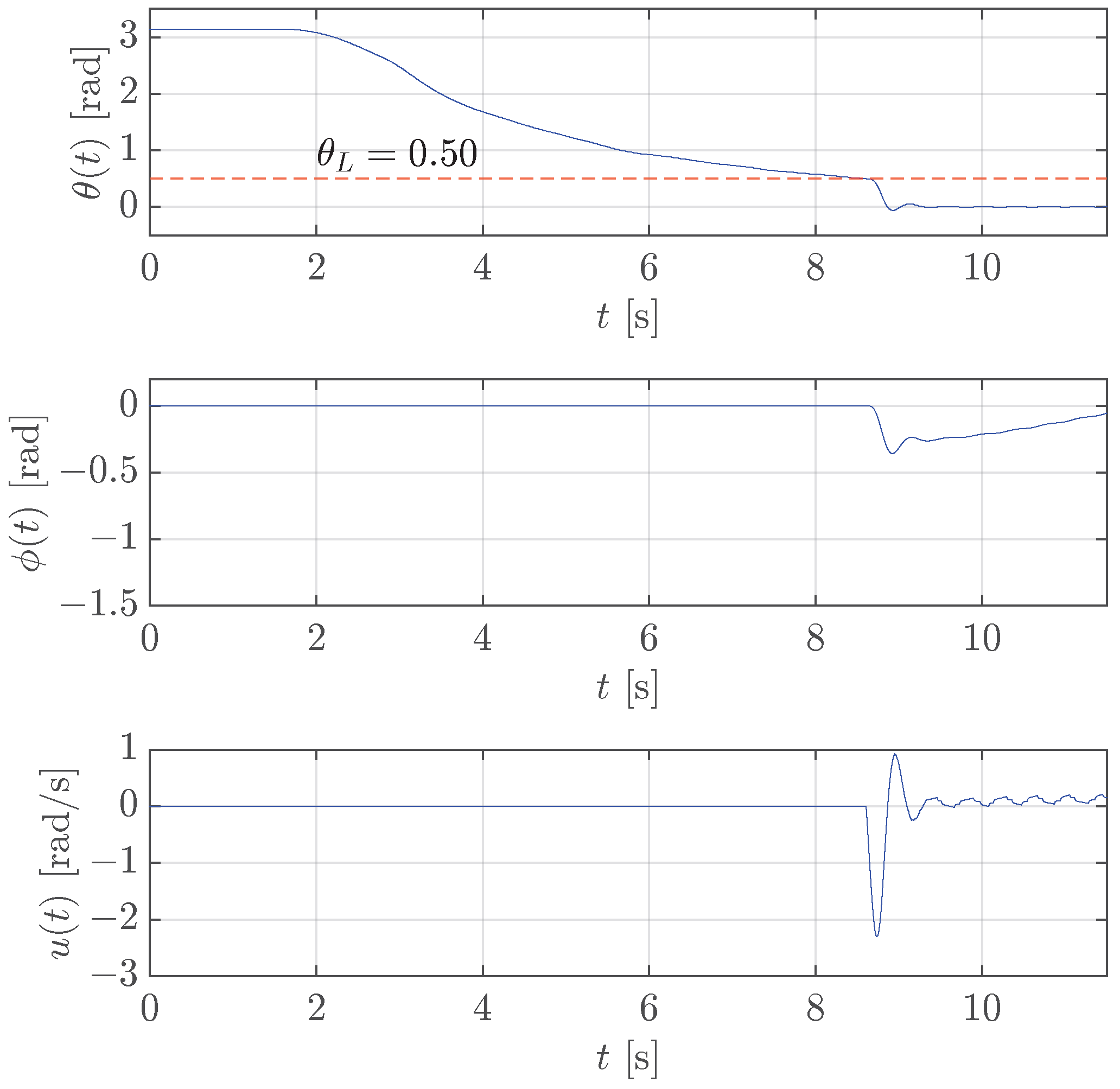
The results in Figure 6 show that stabilization is successful with a threshold rad. In fact, as soon as the pendulum angle reaches the threshold , the control input quickly increases by moving the rotating arm in the right direction to keep the pendulum upright with the expected small quick oscillations of the rotating arm (see the control velocity after 10 s). At the same time, but with a much slower behaviour, the rotating arm angle goes to the desired value 0 that corresponds to the middle of the allowed range.
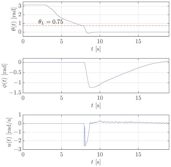
Figure 6.
Case study 1: test of the stabilization control for rotary pendulum with rad (red dashed line).
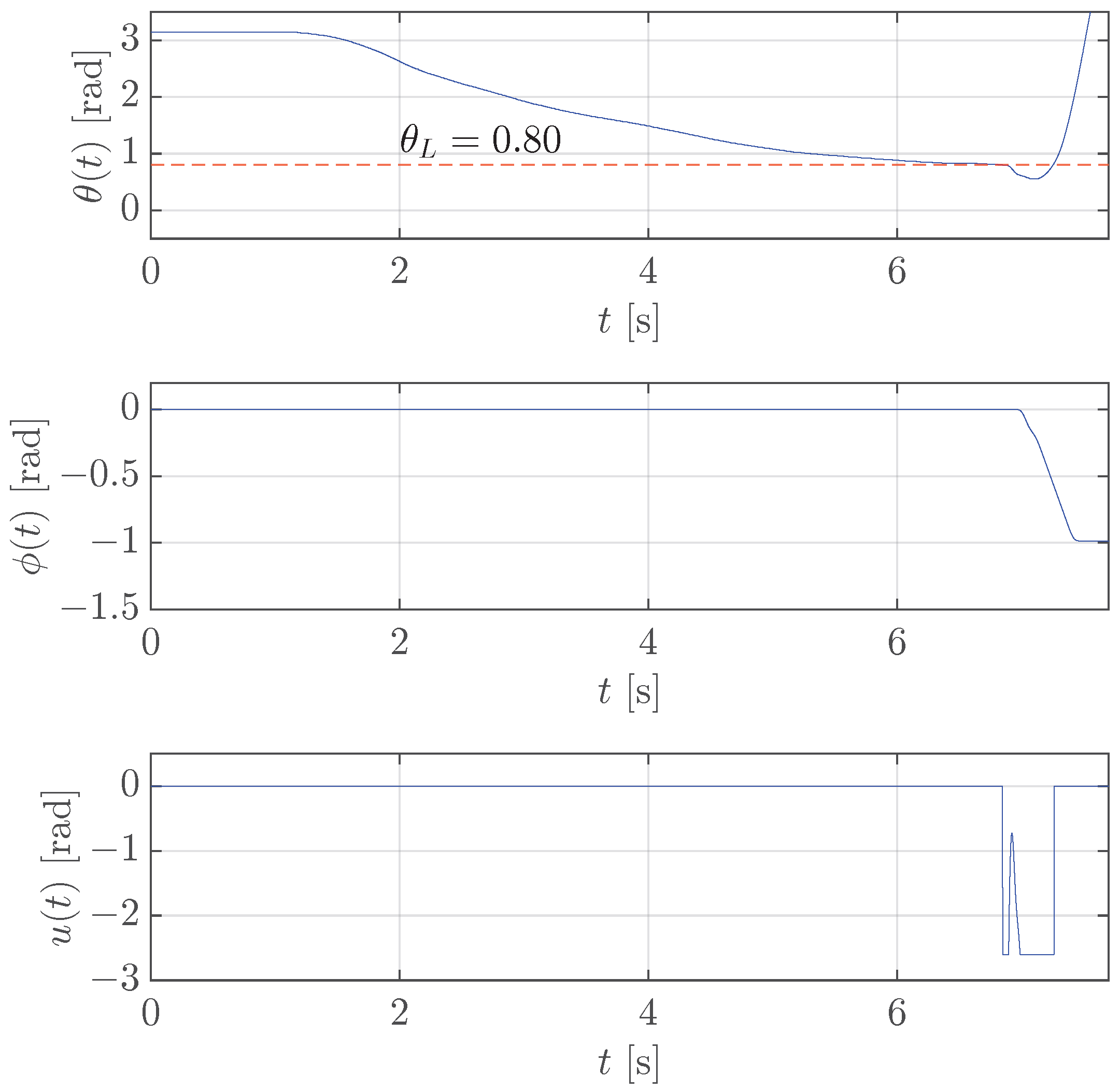
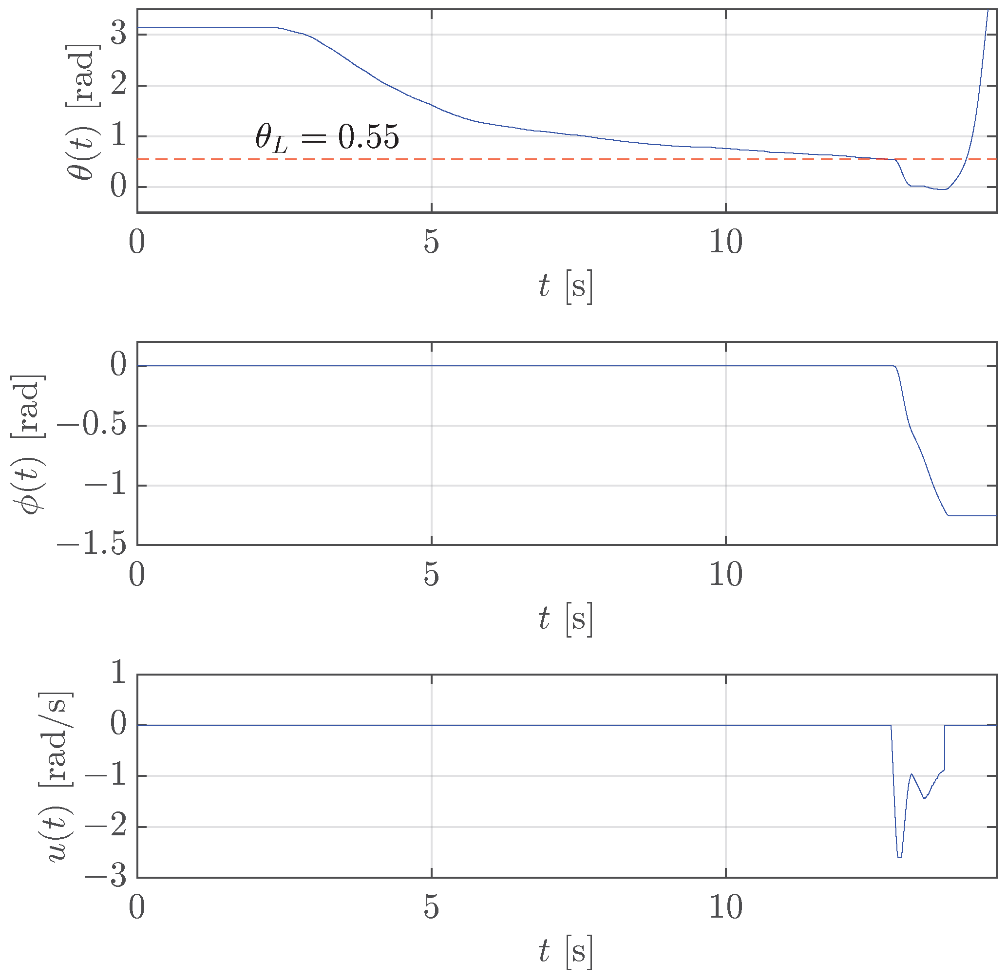
To prove that rad is the maximum allowed value, is increased to rad, and the results in Figure 7 show that the controller is no longer able to stabilize the pendulum as it falls (see the angle that quickly goes to rad at the end of the experiment).
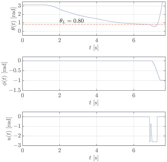
Figure 7.
Case study 1: test of the stabilization control for rotary pendulum with rad (red dashed line).
The LQG controller presented in Section 2.4.1 for the translational pendulum has been designed using the following weights:
The resulting vector gain is
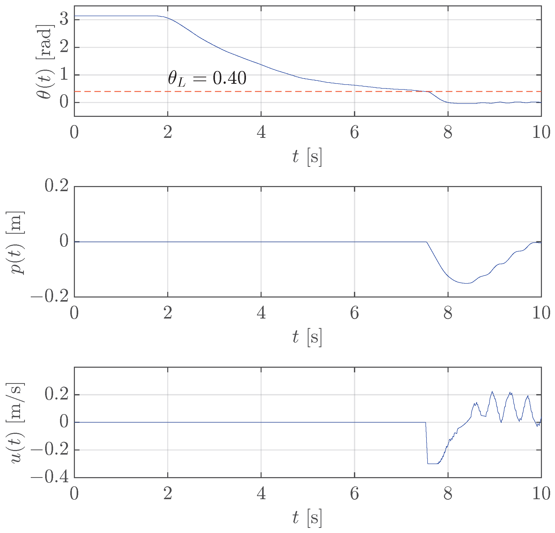
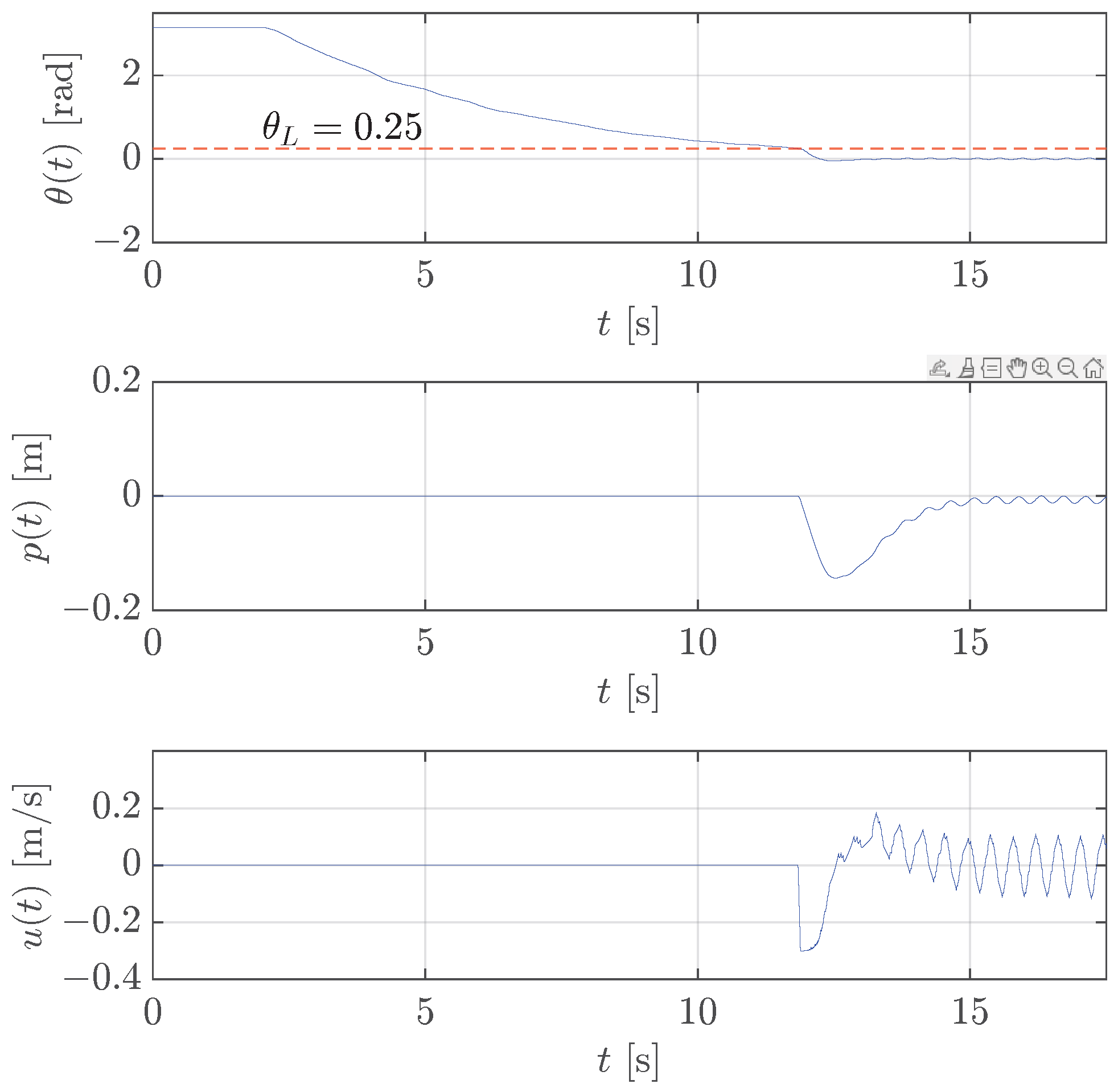
The previous procedure has been executed for the translational pendulum too. Figure 8 illustrates that the controller is activated under the threshold rad, which allows for the pendulum stabilization.
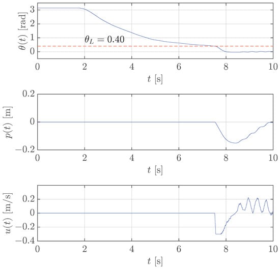
Figure 8.
Case study 1: test of the stabilization control for translational pendulum with rad (red dashed line).
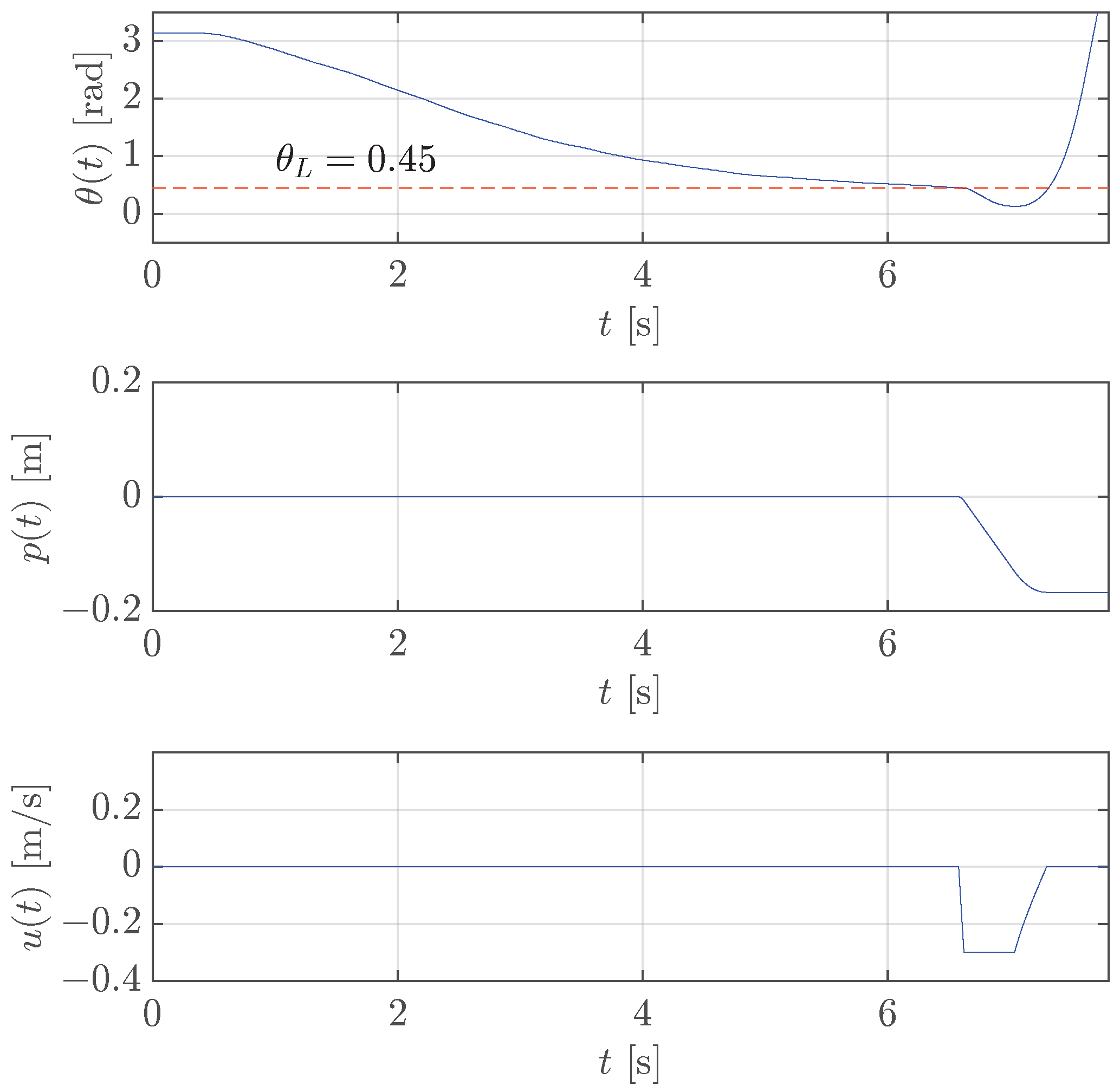
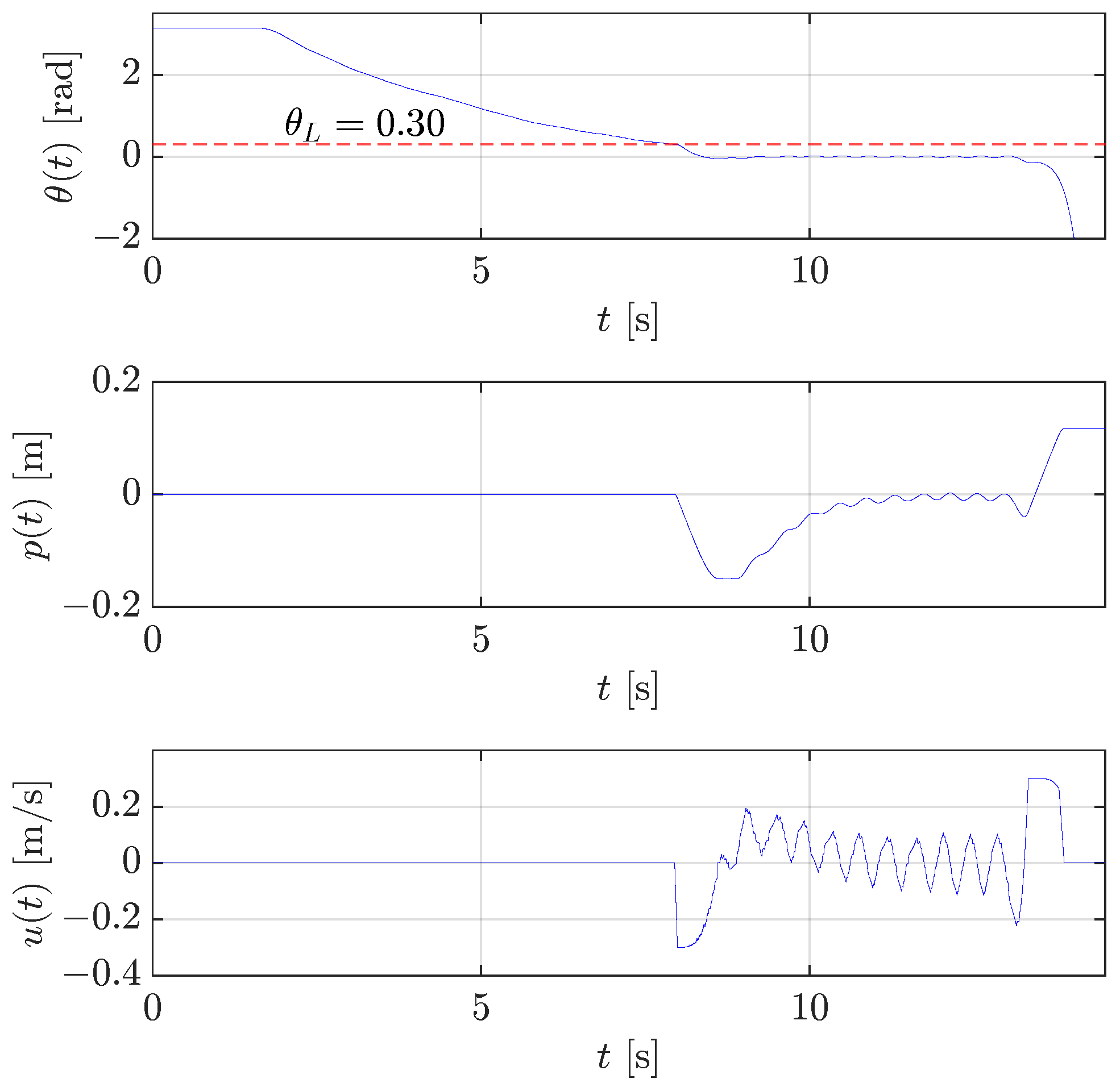
In contrast, the results in Figure 9 show the failure of the stabilization controller using a threshold rad; in fact, the pendulum angle rapidly goes towards rad as soon as the control is activated because the control signal is not quick enough to prevent the pendulum fall.
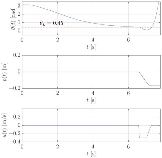
Figure 9.
Case study 1: test of the stabilization control for translational pendulum with rad (red dashed line).
3.2. Case Study 2
The experiments presented in this case study aim to emphasize how important the inclusion of the robot velocity loop dynamics in the stabilization control design is. In fact, the maximum threshold that allows the control to stabilize the pendulum is lower if the controller is designed by neglecting the velocity loop dynamics and the input delay of the control interface.
With reference to the rotary pendulum only (the translational pendulum case is analogous), the simplified open-loop dynamics that assume an instantaneous velocity loop with no input delay can be obtained from the equation of motion (11) with the following definition of the state variables:
Note that the input of this open-loop system is the acceleration ; the actual velocity control input of the robot u can be trivially obtained by time integration.
In this case, the LQG controller presented in Section 2.4.1 for the rotary pendulum has been designed using the following weights:
The resulting vector gain is
Figure 10 demonstrates that the threshold allowing the stabilization is lower than the one used in Figure 6 where the control law was designed by taking into account the full dynamics.
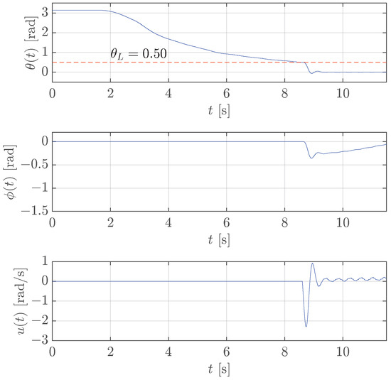
Figure 10.
Case study 2: test of the stabilization control for rotary pendulum with rad (red dashed line), neglecting the robot velocity loop dynamics.
As usual, to prove that the value above is the maximum achievable, the threshold is increased to rad, and Figure 11 shows that the stabilization control fails (the pendulum falls as shown by the angle going towards rad).
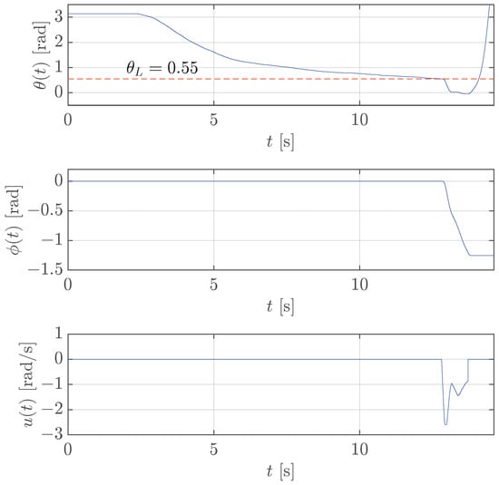
Figure 11.
Case study 2: test of the stabilization control for rotary pendulum with rad (red dashed line), neglecting the robot velocity loop dynamics.
The same test is repeated for the translational pendulum too, and the LQG controller presented in Section 2.4.1 has been designed by neglecting the velocity loop dynamics using the following weights:
The resulting vector gain is
The results clearly demonstrate that the robot velocity loop dynamics affect the stabilization of the translational pendulum too. In fact, Figure 12 proves the success of the stabilization control with a threshold rad, which is lower than the one used in Figure 8 where the controller was designed by taking into account the full system dynamics.
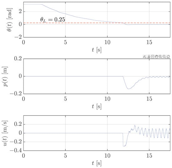
Figure 12.
Case study 2: test of the stabilization control for translational pendulum with rad (red dashed line), neglecting the robot velocity loop dynamics.
Finally, Figure 13 shows that the stabilization control fails by a small increase in the threshold to the value rad.
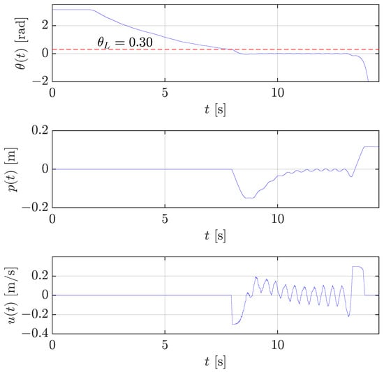
Figure 13.
Case study 2: test of the stabilization control for translational pendulum with rad (red dashed line), neglecting the robot velocity loop dynamics.
3.3. Case Study 3
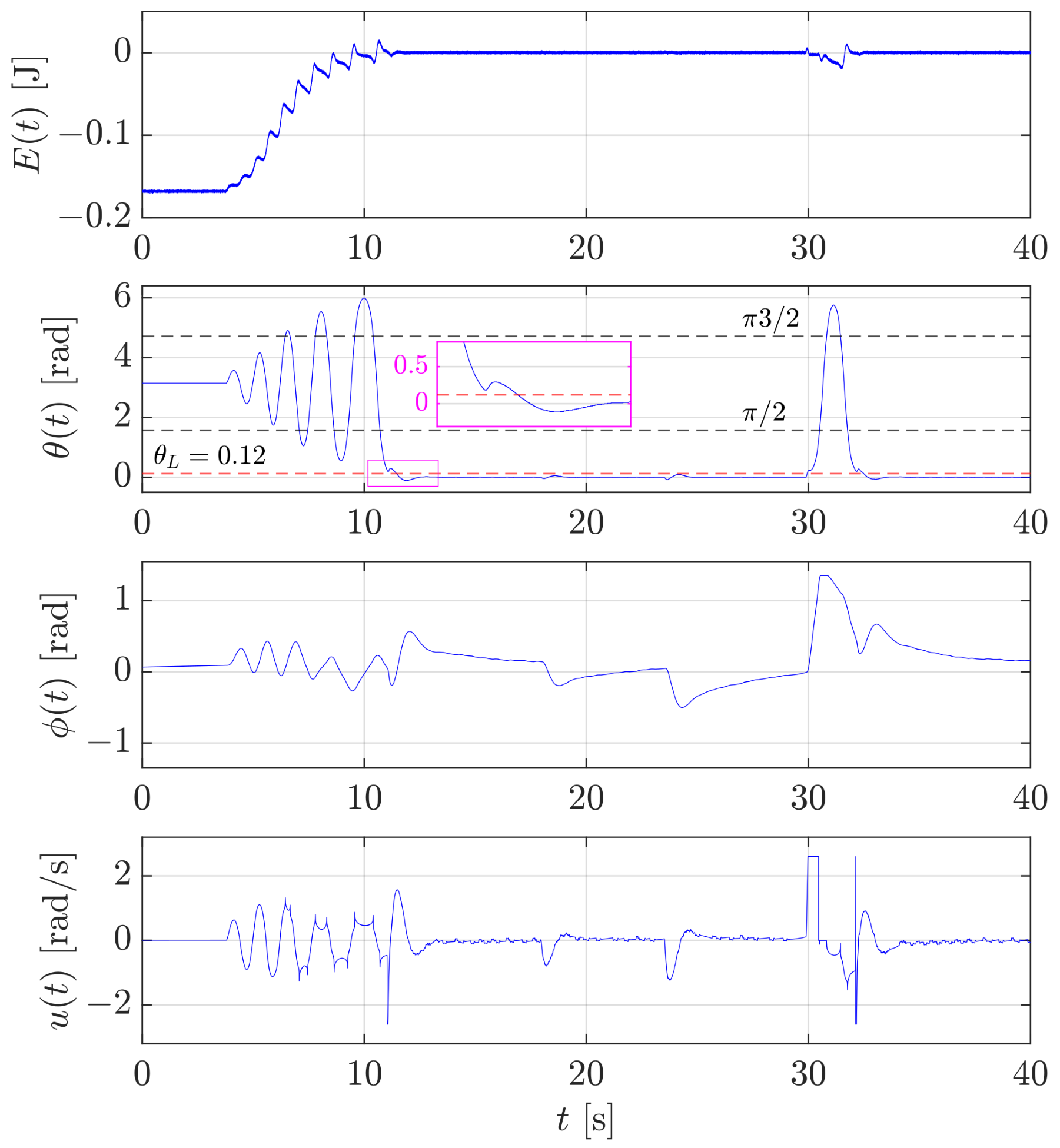
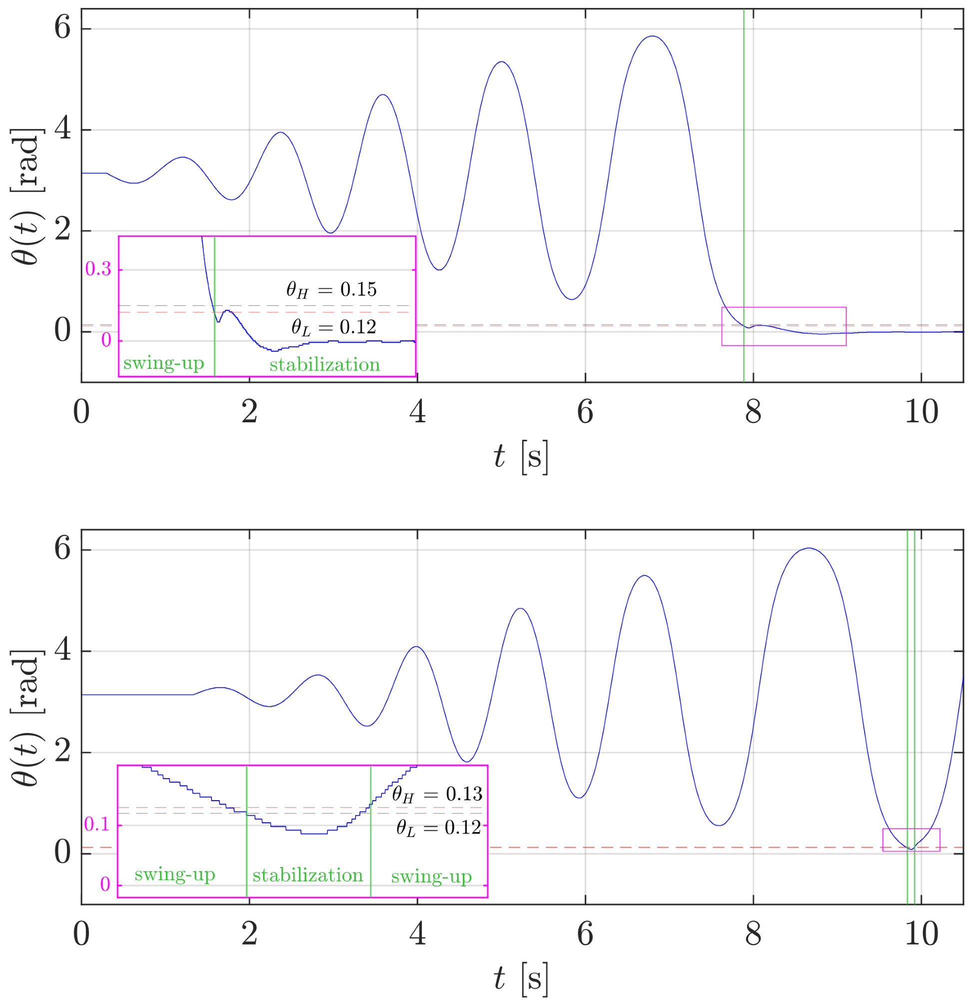
While case study 2 illustrates the relevance of the robot velocity loop dynamics, case study 3 presents the experimental results for the whole control system that includes both the swing-up and the stabilization controllers with the switching strategy discussed in Section 2.4.4. The stabilization control used here is the one designed by considering the robot dynamics for both rotary and translational pendulums, with a common threshold rad. The energy-based swing-up controller for the rotary pendulum in (41) is tuned with a gain and a regularization threshold in (43) , while the swing-up controller for the translational pendulum in (44) is implemented with a gain and a regularization threshold in (46) with the same value as before.
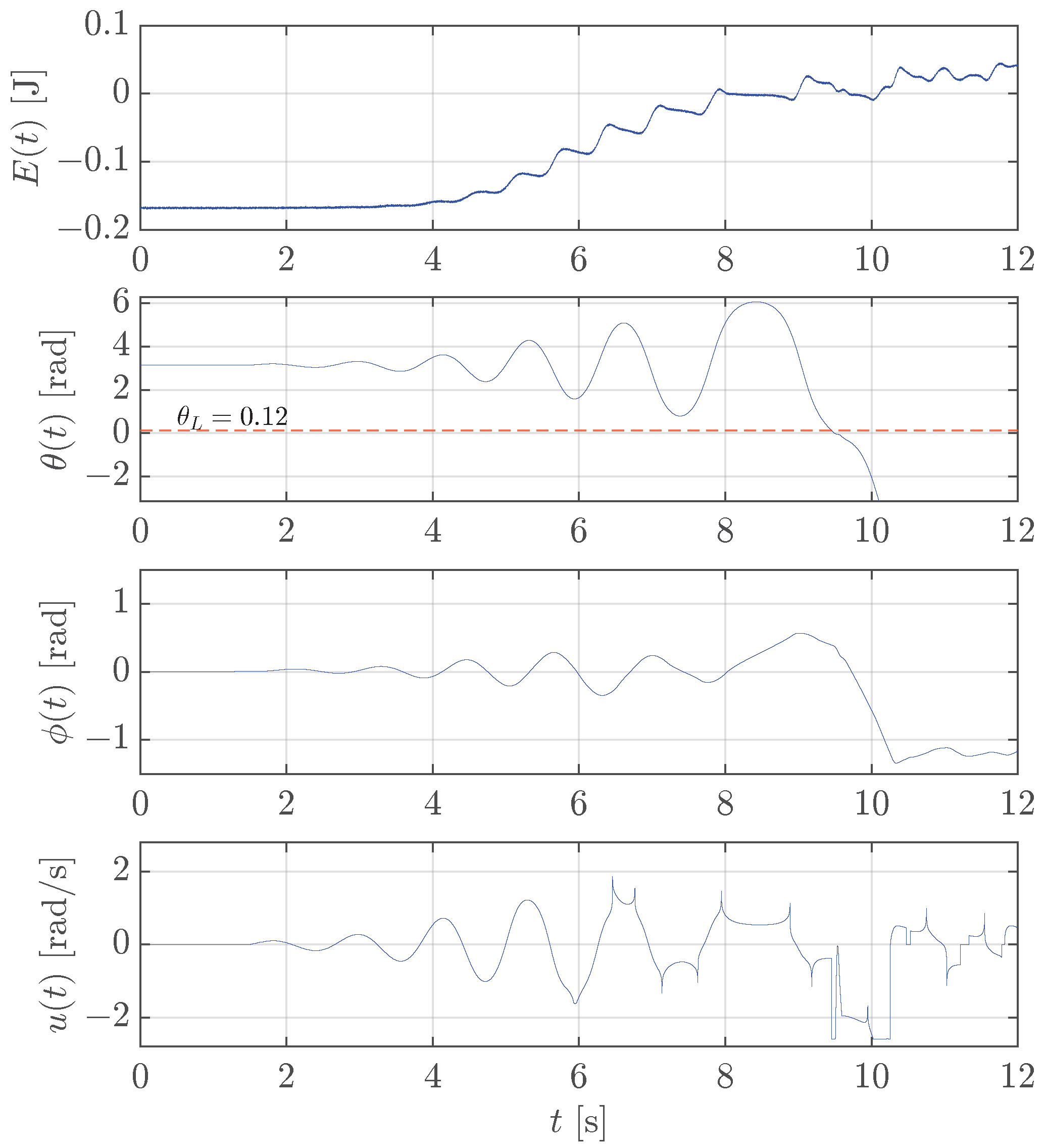
Figure 14 shows the results obtained for the rotary pendulum. The experiment starts when the pendulum is disturbed from its naturally stable position; so, as explained in Section 2.4.2, the energy-based control increases the energy from a negative value up to 0. The energy is computed on the basis of the estimated angular velocity of the pendulum ; therefore, it is affected by noise. During energy-based control, the pendulum swings, and as soon as (see the zoom in the magenta subplot) the stabilization control is activated, and the pendulum is kept upright by a proper motion of the robot. It is worth noticing that the energy in the top plot is not strictly increasing towards zero. At the beginning, during the first two oscillations, there are time instants such that , which is unsurprising because these correspond to , which yields in (42). Surprisingly, the subsequent oscillations are characterized by a non-monotonic energy. This seems to violate the condition that has been proved in Section 2.4.2. This is due to the regularization (43); in fact the energy decreases around and where . At s and s, the operator applies a disturbance to the pendulum, which is fully rejected by the stabilization controller that keeps the pendulum upright. At s, a third and much larger disturbance is applied so that the pendulum falls down because the angle exceeds the threshold in Figure 5. Hence, the energy-based control is automatically re-activated and the robot moves in such a way to bring the pendulum angle below the threshold again, allowing the stabilization controller to keep it upright.
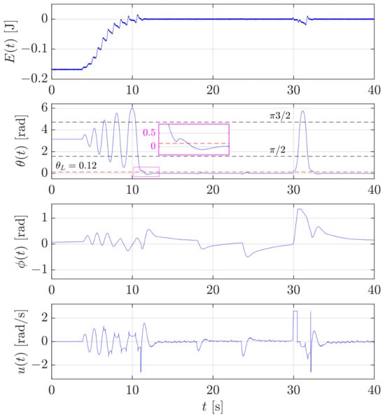
Figure 14.
Case study 3: test of the swing-up control for the rotary pendulum and switching to the stabilization control and vice-versa.
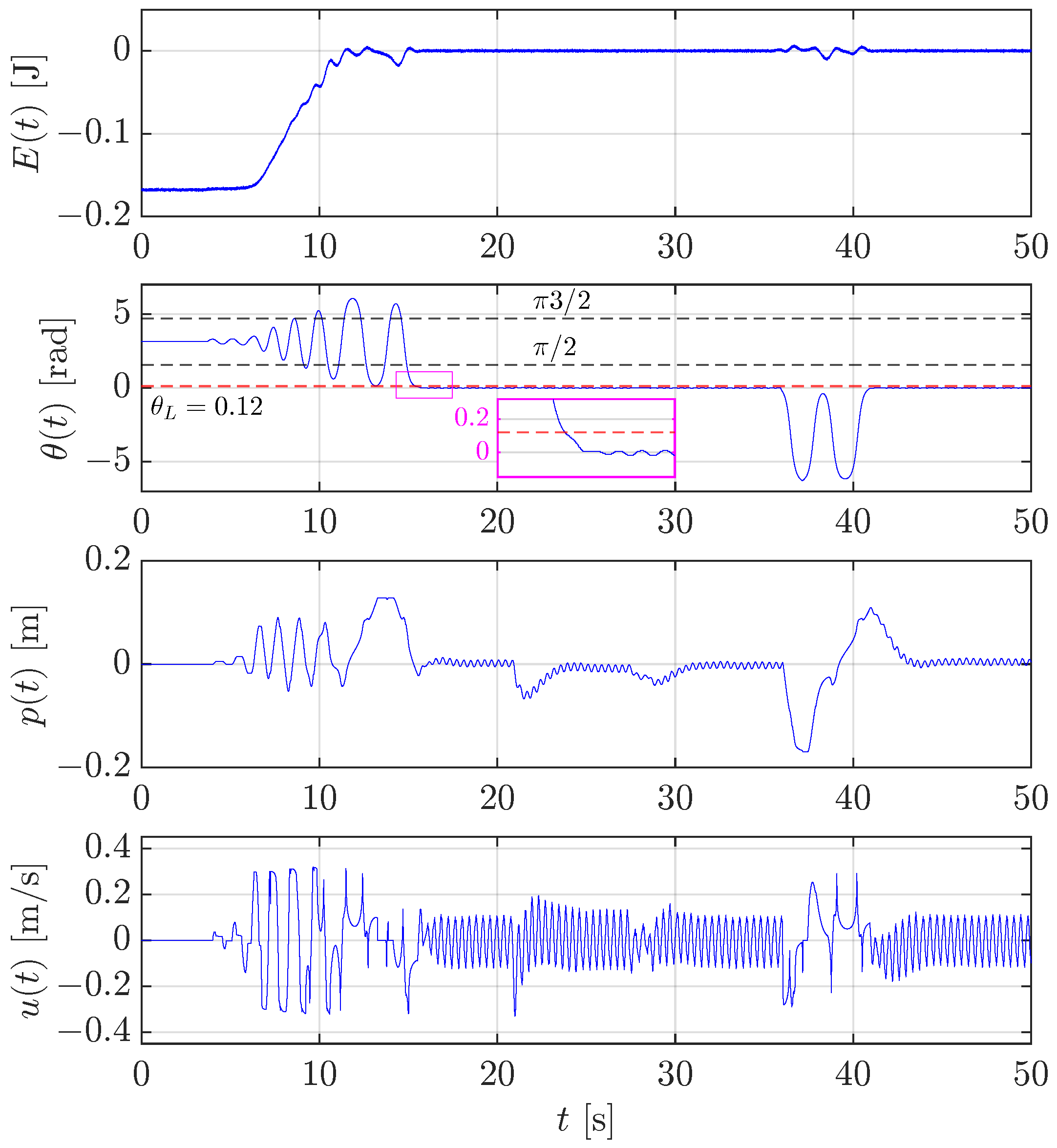
Figure 15 shows the results obtained in a similar experiment executed with the translational pendulum to test the swing-up control described in Section 2.4.3. As already shown in Figure 14 thanks to the zoom in the magenta box, when , the stabilization controller (see Section 3.1) is able to keep the pendulum in the upright position. Again, a disturbance is applied twice at s and s, which is successfully rejected by the stabilization controller. At s, a disturbance large enough is applied to let the pendulum angle exit from the dead zone , and the swing-up controller swings the pendulum twice to let go below again, and the stabilization controller keeps the pendulum upright.
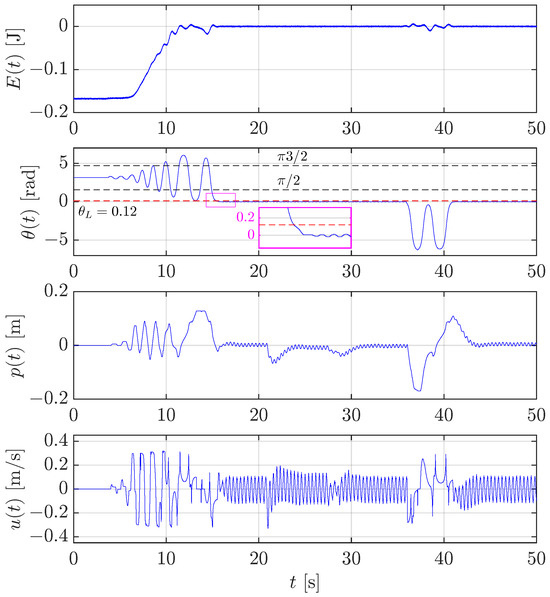
Figure 15.
Case study 3: test of the swing-up control for the translational pendulum and switching to the stabilization control and vice-versa.
3.4. Sensitivity Analysis
The experiments in this section have a dual purpose. The first one is to demonstrate that friction compensation influences the success of the swing-up control law. The second one is focused on the design of the threshold to avoid unexpected switches of the control strategy. For brevity, the results shown below regard the rotary pendulum only, with a threshold rad similar to the one selected in Section 3.3.
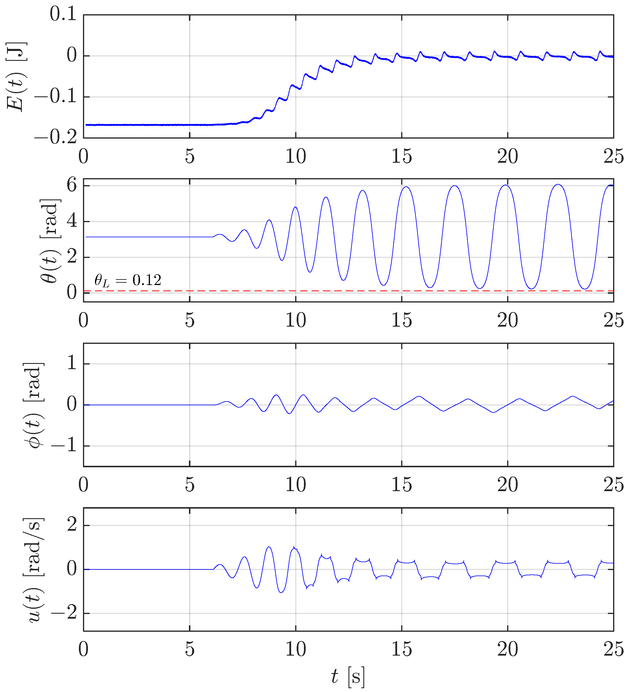
Regarding the friction compensation, several experiments have been conducted by varying the friction coefficient that led us to find the lower and upper limits within which the friction coefficient used in the friction compensation (43) granted the success of the swing-up control. Figure 16 shows the results in the case the friction is under-compensated with a value of the friction coefficient in (43) equal to , with representing the nominal value in Table 1. Even if the energy is brought to 0 J, the swing-up control law is not capable of bringing the pendulum angle below the threshold rad as it is needed to switch the control mode to the stabilization control. In conclusion, after the first part of the experiment (from s to s) when the energy is increasing, the pendulum continues to oscillate without approaching the upright position close enough to trigger the stabilization.
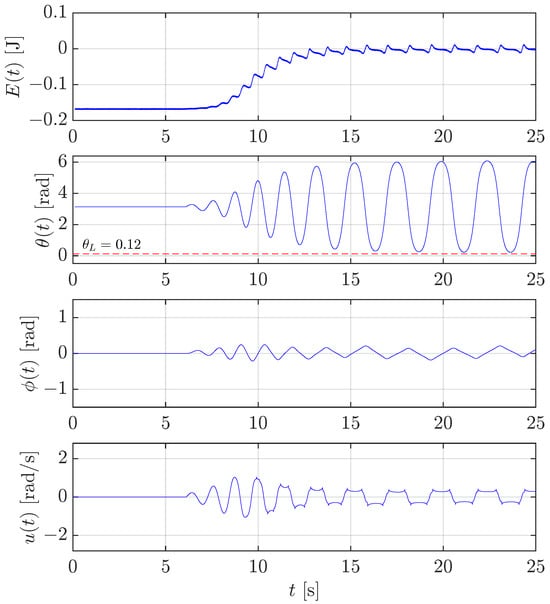
Figure 16.
Sensitivity analysis: test of the swing-up control for the rotary pendulum with friction compensation implemented with a friction coefficient equal to of its nominal value.
On the other hand, Figure 17 reports the results in the case the friction is over-compensated with the upper limit value of , with representing the nominal friction coefficient in Table 1. The overcompensation leads the swing-up control to bring the energy significantly over 0 J ( s) so that the pendulum enters the stabilization range with too much velocity, and the controller is unable to stabilize the system.
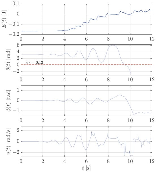
Figure 17.
Sensitivity analysis: test of the swing-up control for the rotary pendulum with friction compensation implemented with a friction coefficient equal to of its nominal value.
Regarding the sensitivity with respect to the threshold , Figure 18 reports the behaviour of the angle with different choices of the threshold . The upper plot illustrates the case in which rad, selected as discussed in Section 2.4.4. With this setting, the switching strategy successfully switches from the swing-up to the stabilization control. In fact, as highlighted in the magenta subplot, after the stabilization control mode is activated, the closed-loop system dynamics are such that the angle exceeds the switching threshold but not .
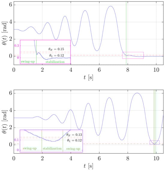
Figure 18.
Sensitivity analysis: test of the swing-up control for the rotary pendulum with two different values of the threshold ( rad in the top plot; in the bottom plot). The vertical green lines highlight the switching instants of the control mode.
The lower plot shows the case of a more narrow non-switching zone, i.e., rad. The results of this choice are emphasized by the magenta subplot and the two vertical green lines. With the swing-up controller active, as soon as the angle reaches the lower threshold , the stabilization controller starts. However, the stabilization fails because, during the transient, the angle overcomes the threshold , triggering the switch to the swing-up control.
4. Discussion
The results presented in the previous section clearly demonstrate that the control of an inverted pendulum can be successfully achieved even in the presence of a velocity-controlled actuation system (in this paper, a six-joint robot) rather than a torque-controlled one as most of the solutions in the related literature propose. However, the results also show that the performance of the stabilization control of the pendulum significantly depends on the quality of the dynamic model used in the design. In fact, the estimates of the region of attraction summarized in Table 2 prove that the LQG controllers designed by neglecting the velocity loop dynamics and the input delay introduced by the digital control interface of the robot are significantly smaller than those estimated for the LQG controllers designed by considering the complete model of the system. Another advantage offered by a velocity-controlled actuation system of the pendulum consists in the possibility to apply the same control law to a wider set of actuation systems, independently from their dynamic parameters.
Table 2.
Summary of the region of attraction estimate [rad] achieved by the stabilization controller—(R) refers to the rotary pendulum; (T) refers to the translational pendulum.
Another aspect of interest of the present work is that it explicitly considers in the design of the swing-up control law the friction on the pendulum axis, which is usually neglected in the literature since it establishes a controllability problem. In fact, the dynamic equations clearly show that the control input vanishes for rad, and thus a full friction compensation is impossible. The problem has been partially overcome here by resorting to a regularization technique. Nevertheless, the technique has been shown to be effective even with a partially known friction coefficient, as demonstrated by the sensitivity analysis conducted with respect to this parameter. The same analysis also clearly shows that a swing-up without friction compensation is impossible. Future studies will be devoted to investigating more general solutions and to tackling the problem of the robustness of the swing-up control strategy with respect to other parameters; actually, preliminary experiments showed that overestimation of the moment of inertia of the pendulum can negatively affect the swing-up effectiveness.
Eventually, the model-based control approach followed in this paper will be compared to reinforcement learning strategies to understand if their generalization capabilities and robustness property to the most uncertain parameters, like friction, are enough to control inverted pendulums with different physical parameters without the need to retrain the control policy.
Supplementary Materials
The following supporting information can be downloaded at: https://www.mdpi.com/article/10.3390/machines13060528/s1.
Author Contributions
Conceptualization, M.C. and C.N.; methodology, C.N.; software, R.M.; validation, M.C., R.M. and C.N.; formal analysis, M.C. and C.N.; resources, M.C.; data curation, R.M.; writing—original draft preparation, C.N.; writing—review and editing, M.C., R.M. and C.N.; visualization, R.M.; supervision, C.N.; funding acquisition, M.C. All authors have read and agreed to the published version of the manuscript.
Funding
This work was supported by the Italian Ministry of Scientific Research under the PRIN2022 PNRR (DARC Project) under Grant P2022MHR5C.
Data Availability Statement
All the data produced in this research are those reported in the plots.
Conflicts of Interest
The authors declare no conflicts of interest.
References
- Hoshino, T.; Yamakita, M.; Furuta, K. Control Education Using Pendulum Apparatus. Trans. Control Autom. Syst. Eng. 2000, 2, 157–162. [Google Scholar]
- Jensen, N.J.; Ishizaki, T. Furuta Pendulum Design Update for Accessible Control Demonstrations. IFAC-PapersOnLine 2023, 56, 7573–7578. [Google Scholar] [CrossRef]
- Hehn, M.; D’Andrea, R. A flying inverted pendulum. In Proceedings of the 2011 IEEE International Conference on Robotics and Automation, Shanghai, China, 9–13 May 2011; pp. 763–770. [Google Scholar] [CrossRef]
- Anh, N.; Matsuhisa, H.; Viet, L.; Yasuda, M. Vibration control of an inverted pendulum type structure by passive mass–spring-pendulum dynamic vibration absorber. J. Sound Vib. 2007, 307, 187–201. [Google Scholar] [CrossRef]
- Grasser, F.; D’Arrigo, A.; Colombi, S.; Rufer, A. JOE: A mobile, inverted pendulum. IEEE Trans. Ind. Electron. 2002, 49, 107–114. [Google Scholar] [CrossRef]
- Boubaker, O. The Inverted Pendulum Benchmark in Nonlinear Control Theory: A Survey. Int. J. Adv. Robot. Syst. 2013, 10, 233. [Google Scholar] [CrossRef]
- Vizi, M.B.; Stepan, G. Stability of the Furuta pendulum with delayed digital controller. IFAC-PapersOnLine 2021, 54, 204–208. [Google Scholar] [CrossRef]
- Alves, U.N.L.T.; Breganon, R.; Pivovar, L.E.; de Almeida, J.P.L.S.; Barbara, G.V.; Mendonça, M.; Palácios, R.H.C. Discrete-Time H∞ Integral Control Via LMIs Applied to a Furuta Pendulum. J. Control Autom. Electr. Syst. 2022, 33, 1–12. [Google Scholar] [CrossRef]
- Seman, P.; Rohal’-Ilkiv, B.; Juh´as, M.; Salaj, M. Swinging up the Furuta Pendulum and its Stabilization Via Model Predictive Control. J. Electr. Eng. 2013, 64, 152–158. [Google Scholar] [CrossRef]
- Aracil, J.; Acosta, J.; Gordillo, F. A nonlinear hybrid controller for swinging-up and stabilizing the Furuta pendulum. Control Eng. Pract. 2013, 21, 989–993. [Google Scholar] [CrossRef]
- Aguilar-Avelar, C.; Moreno-Valenzuela, J. New Feedback Linearization-Based Control for Arm Trajectory Tracking of the Furuta Pendulum. IEEE/ASME Trans. Mech. 2016, 21, 638–648. [Google Scholar] [CrossRef]
- Yan, Q. Output tracking of underactuated rotary inverted pendulum by nonlinear controller. In Proceedings of the 42nd IEEE International Conference on Decision and Control (IEEE Cat. No.03CH37475), Maui, HI, USA, 9–12 December 2003; Volume 3, pp. 2395–2400. [Google Scholar] [CrossRef]
- Bellati, A.; Blengio, N.P.; Cancela, F.; Monzón, P.; Pérez, N. Modeling and control of a Furuta pendulum. In Proceedings of the 2021 IEEE URUCON, Montevideo, Uruguaym, 24–26 November 2021; pp. 334–338. [Google Scholar] [CrossRef]
- Åström, K.; Furuta, K. Swinging up a pendulum by energy control. Automatica 2000, 36, 287–295. [Google Scholar] [CrossRef]
- Park, M.S.; Chwa, D. Swing-Up and Stabilization Control of Inverted-Pendulum Systems via Coupled Sliding-Mode Control Method. IEEE Trans. Ind. Electron. 2009, 56, 3541–3555. [Google Scholar] [CrossRef]
- Muskinja, N.; Tovornik, B. Swinging up and stabilization of a real inverted pendulum. IEEE Trans. Ind. Electron. 2006, 53, 631–639. [Google Scholar] [CrossRef]
- Susanto, E.; Surya Wibowo, A.; Ghiffary Rachman, E. Fuzzy Swing Up Control and Optimal State Feedback Stabilization for Self-Erecting Inverted Pendulum. IEEE Access 2020, 8, 6496–6504. [Google Scholar] [CrossRef]
- Vizi, M.B.; Stepan, G. Digital stability of the Furuta pendulum based on angle detection. J. Vib. Control 2024, 30, 588–597. [Google Scholar] [CrossRef]
- Zhang, L.; Ning, Z.; Shi, Y. Analysis and synthesis for a class of stochastic switching systems against delayed mode switching: A framework of integrating mode weights. Automatica 2019, 99, 99–111. [Google Scholar] [CrossRef]
- Xenomai. Xenomai Real-Time Framework. 2024. Available online: https://v3.xenomai.org/overview/ (accessed on 5 May 2025).
- Barut, S.; Boneberger, M.; Mohammadi, P.; Steil, J.J. Benchmarking Real-Time Capabilities of ROS 2 and OROCOS for Robotics Applications. In Proceedings of the 2021 IEEE International Conference on Robotics and Automation (ICRA), Xi’an, China, 30 May–5 June 2021; pp. 708–714. [Google Scholar] [CrossRef]
- Delgado, R.; You, B.J.; Choi, B.W. Real-time control architecture based on Xenomai using ROS packages for a service robot. J. Syst. Softw. 2019, 151, 8–19. [Google Scholar] [CrossRef]
- Gäfvert, M. Modelling the Furuta Pendulum; Technical Reports TFRT-7574; Department of Automatic Control, Lund Institute of Technology (LTH): Lund, Sweden, 1998. [Google Scholar]
- Siciliano, B. Kinematic control of redundant robot manipulators: A tutorial. J. Intell. Robot. Syst. 1990, 3, 201–212. [Google Scholar] [CrossRef]
- Siciliano, B.; Sciavicco, L.; Villani, L.; Oriolo, G. Robotics: Modelling, Planning and Control; Springer Publishing Company, Incorporated: London, UK, 2010. [Google Scholar]
- Mills, A.; Wills, A.; Ninness, B. Nonlinear model predictive control of an inverted pendulum. In Proceedings of the 2009 American Control Conference, St. Louis, MO, USA, 10–12 June 2009; pp. 2335–2340. [Google Scholar] [CrossRef]
- Grewal, M.S.; Andrews, A.P. Kalman Filtering: Theory and Practice with MATLAB, 4th ed.; Wiley-IEEE Press: Hoboken, NJ, USA, 2014. [Google Scholar]
- Lewis, F.L.; Vrabie, D.L.; Syrmos, V.L. Optimal Control; John Wiley & Sons, Inc.: Hoboken, NJ, USA, 2012. [Google Scholar] [CrossRef]


Disclaimer/Publisher’s Note: The statements, opinions and data contained in all publications are solely those of the individual author(s) and contributor(s) and not of MDPI and/or the editor(s). MDPI and/or the editor(s) disclaim responsibility for any injury to people or property resulting from any ideas, methods, instructions or products referred to in the content. |
© 2025 by the authors. Licensee MDPI, Basel, Switzerland. This article is an open access article distributed under the terms and conditions of the Creative Commons Attribution (CC BY) license (https://creativecommons.org/licenses/by/4.0/).