Article

How to Win Bosch Future Mobility Challenge: Design and Implementation of the VROOM Autonomous Scaled Vehicle

by
Theodoros Papafotiou
1,
Emmanouil Tsardoulias
1,*,
Alexandros Nikolaou
1,
Aikaterini Papagiannitsi
1,
Despoina Christodoulou
2,
Ioannis Gkountras
1 and
Andreas L. Symeonidis
1
1
School of Electrical and Computer Engineering, Faculty of Engineering, Aristotle University of Thessaloniki (AUTh), 54124 Thessaloniki, Greece
2
Department of Applied Informatics, University of Macedonia, 54636 Thessaloniki, Greece
*
Author to whom correspondence should be addressed.
Machines 2025, 13(6), 514; https://doi.org/10.3390/machines13060514
Submission received: 16 April 2025 / Revised: 28 May 2025 / Accepted: 10 June 2025 / Published: 12 June 2025
(This article belongs to the Special Issue Emerging Approaches to Intelligent and Autonomous Systems)

Abstract

Over the last decade, a transformation in the automotive industry has been witnessed, as advancements in artificial intelligence and sensor technology have continued to accelerate the development of driverless vehicles. These systems are expected to significantly reduce traffic accidents and associated costs, making their integration into future transportation systems highly impactful. To explore this field in a controlled and flexible manner, scaled autonomous vehicle platforms are increasingly adopted for experimentation. In this work, we propose a set of methodologies to perform autonomous driving tasks through a software–hardware co-design approach. The developed system focuses on deploying a modular and reconfigurable software stack tailored to run efficiently on constrained embedded hardware, demonstrating a balance between real-time capability and computational resource usage. The proposed platform was implemented on a 1:10 scale vehicle that participated in the Bosch Future Mobility Challenge (BFMC) 2024. It integrates a high-performance embedded computing unit and a heterogeneous sensor suite to achieve reliable perception, decision-making, and control. The architecture is structured across four interconnected layers—Input, Perception, Control, and Output—allowing flexible module integration and reusability. The effectiveness of the system was validated throughout the competition scenarios, leading the team to secure first place. Although the platform was evaluated on a scaled vehicle, its underlying software–hardware principles are broadly applicable and scalable to larger autonomous systems.

1. Introduction

Autonomous driving technology has rapidly evolved in recent years, holding the potential to revolutionize mobility by enhancing road safety, reducing congestion, and improving energy efficiency. Autonomous vehicles (AVs) are equipped with advanced sensors, artificial intelligence (AI)-driven perception systems, and real-time decision-making algorithms, allowing them to efficiently navigate complex environments with minimal human intervention.
Autonomous cars are poised to transform the future of transportation by addressing critical issues such as road safety, traffic efficiency, and cost reduction. Human error accounts for around 94% of road accidents [1], and autonomous vehicles, with their advanced sensors and AI-driven decision-making, can dramatically reduce this figure, saving hundreds of thousands of lives annually [2]. Autonomous vehicles could also optimize traffic flow, reducing congestion and leading to less commute time and, at the same time, the more efficient delivery of goods and services, cutting operational costs for businesses and boosting productivity across sectors [3].
Implementing autonomous vehicles presents a series of complex challenges, particularly in achieving robust perception and decision-making in dynamic urban environments. These systems must process and fuse data from diverse sensors in real time to detect, classify, and respond to objects and events. They must also operate reliably in unpredictable conditions like poor weather, sudden obstacles, or erratic behavior from other agents. Alongside algorithmic complexity, ensuring consistent power delivery, maintaining low latency, and verifying safety across edge-case scenarios demand careful system design and extensive testing, both in simulation and physical environments.
In parallel with full-scale AV development, 1:10 scale models play a pivotal role in research and development. These scaled-down models offer cost-effective and flexible testbeds for evaluating algorithms, validating vehicle behaviors, and simulating real-world scenarios in controlled environments. Their relevance lies in their ability to replicate the dynamics of full-sized AVs while enabling faster iterations and safer experimentation, making them an essential tool in advancing autonomous driving systems. Of course, vehicle simulators exist as well; nevertheless, their realism falls behind the real-life scaled environments, which in turn are less realistic than the real world.
This paper addresses a key research gap: the lack of robust autonomous driving software that is both modular and capable of running efficiently on computationally constrained embedded platforms with minimal sensor configurations. The primary objective of this work is to develop and evaluate a complete software/hardware co-design-driven framework that enables autonomous operation under real-time conditions in scaled urban environments. Specifically, the focus is on designing efficient perception, decision-making, and control modules that allow the vehicle to autonomously navigate while adhering to safety, efficiency, and real-time constraints. The system is intended to handle real-world tasks such as obstacle detection and identification, vehicle interaction, and lane-keeping, with the ability to dynamically adapt its path in response to changing conditions. A key aspect of this work is the use of a 1:10 scale autonomous vehicle model, which enables the thorough testing of algorithms in a controlled yet realistic environment.
The relevance of this research to the Bosch Future Mobility Challenge (BFMC) lies in its alignment with the competition’s core goals, which include demonstrating the ability to autonomously navigate a miniaturized smart city. The vehicle must successfully complete a series of predefined tasks such as intersection management, parking process, and interaction with dynamic obstacles, all while maintaining a high level of safety and efficiency. This research, therefore, aims to directly address the competition’s requirements by optimizing the vehicle’s performance in both task execution and overall system robustness. Furthermore, one of the key restrictions of the competition is that each vehicle cannot cost more than 1000 euros, thus, our approach had to be cost efficient but still operational to realistic conditions.
The remainder of this work is structured as follows. In Section 1 (current section), we introduce the scope, objectives, and background of our research, highlighting the importance of autonomous vehicles and the relevance of scaled models in testing these systems. Section 2 provides a review of the existing literature, focusing on the advancements in autonomous vehicle technologies, the challenges, and the key points in utilizing model-based testing environments. In Section 3, we present an overview of the BFMC, detailing the competition’s structure, specifications, and the significance of the project in this context. Section 4 describes the design, development, and integration of the hardware and software used in the vehicle, outlining key components and algorithms that were implemented to meet the challenge and team requirements. In Section 5 we discuss the results of our work, emphasizing the vehicle’s performance in the competition and analyzing potential improvements. Finally, in Section 6, we summarize our findings, reflect on the implications of our research, and propose potential directions for future work to enhance the vehicle’s scalability, performance, and autonomous capabilities.

2. Literature Review

Autonomous driving refers to the capability of a vehicle to perceive its environment and navigate without human input. This technology has the potential to revolutionize modern transportation by improving safety, enabling mobility for individuals with disabilities, and reducing both environmental impact and traffic congestion through optimized traffic flow. The development of autonomous driving technology has evolved over the decades. One of the earliest projects was the Eureka Project PROMETHEUS [4] in 1987–1995, which focused on advancing technologies for autonomous and semi-autonomous road vehicles. The 2004 DARPA Grand Challenge [5,6] was a groundbreaking race of autonomous vehicles, that aimed to foster the development of self-driving vehicles. Although no vehicle completed the course that year, the challenge laid the foundation for significant advancements in the field. In the subsequent DARPA Urban Challenge in 2007 [7], vehicles had to navigate through an urban environment, marking an important step towards fully autonomous cars. The Society of Automotive Engineers (SAE) has defined six levels of driving automation [8], ranging from Level 0, where the driver is fully in control, to Level 5, where the vehicle can handle every aspect of driving under any conditions. Current advancements are primarily focused on achieving Level 4, where the vehicle can handle all driving tasks under limited conditions without any human intervention.
In autonomous driving, Yurtsever et al. [9] mention that the underlying system architectures can be generally classified into two major approaches: modular systems and end-to-end systems. In modular architectural approaches, the driving task is broken down into sub-tasks, such as localization (where the vehicle determines its position relative to its environment using technologies like Global Positioning System-GPS and Simultaneous Localization and Mapping-SLAM), perception (which uses sensor data from LiDAR, radar, and cameras to identify obstacles, road signs, and other vehicles), planning (where the system generates a safe and efficient driving route based on the vehicle’s surroundings and intended destination), and control (where commands are sent to the vehicle’s actuators to steer, accelerate, or brake). This separation allows the complex problem of automated driving to be tackled as a series of smaller, more manageable problems, each building on existing technology from areas like robotics, computer vision, and vehicle dynamics.
End-to-end approaches aim to simplify the complex task of autonomous driving by directly mapping sensor inputs to driving actions, usually employing deep learning techniques. Companies like Wayve have adopted this approach as demonstrated by their AV2.0 system [10], which leverages deep learning to improve autonomous driving capabilities. There are three main approaches to end-to-end driving: direct supervised deep learning [11,12,13], neuroevolution [14], and deep reinforcement learning [15,16]. The direct supervised deep learning methodology trains a neural network on large datasets of driving scenarios, teaching the system to mimic human driving behavior; neuroevolution optimizes both the structure and the weights of neural networks using evolutionary algorithms; and deep reinforcement learning (DRL) takes a different approach by allowing a model to learn through trial and error within a simulated environment, refining its driving ability based on reward mechanisms for successful actions and penalties for failures. Some approaches combine these methods to enhance robustness and cover a wider range of driving scenarios. For instance, combining imitation learning with reinforcement learning has been shown to improve driving performance by Lu et al. [17].
When autonomous driving aspects are being researched, full-scale autonomous vehicles are often prohibitively expensive, and the associated risks are high. Thus, small-scale car platforms present a practical and compelling alternative that significantly lowers the entry barriers, inviting a diverse group of researchers to engage in autonomous driving research. These models incorporate similar hardware and software components used in real autonomous vehicles, including sensors like LiDARs, cameras, and IMUs, computational units, and actuators. Scaled models often operate within a miniaturized smart city environment that includes traffic lights, road signs, and other urban infrastructure, serving as testbeds in autonomous driving research. The concept behind this approach is that the more realistic the simulation testbed, the more the algorithms can be applied to real-world conditions without major alterations.
Li et al. [18] highlight that the development of scaled models has seen several key projects and milestones. There have been multiple platforms addressing the scientific community, including commercially available options like DeepRacer [19] and Duckietown [20], as well as open-source projects such as DonkeyCar (https://docs.donkeycar.com/, accessed on 9 June 2025). These platforms serve as educational tools for aspiring engineers and developers, introducing them to engineering and autonomous driving technologies. Additionally, research testbeds like BARC [21], along with open-source platforms such as F1TENTH [22] and AutoRally [23], offer robust environments for researchers to conduct advanced studies in autonomous vehicle systems, enabling them to test, refine, and validate their algorithms in a controlled and reproducible manner.
More notably, the F1TENTH platform is a robust and versatile testbed that integrates realistic vehicle dynamics and drivetrain systems, making it a reliable tool for validating algorithms in controlled settings before real-world deployment. It utilizes fully open-source and standardized components that leverage the Robot Operating System (ROS) middleware, supporting a wide range of sensors including LiDARs, monocular and stereo cameras, and inertial measurement units, enabling complex navigation and localization tasks. Research conducted using the F1TENTH platform spans various areas of autonomous vehicle technology, including perception, planning, and control. The platform supports a vibrant community of researchers and educators, contributing to its ongoing development and refinement. The annual F1TENTH Autonomous Racing Competitions [24] further highlight the platform’s capabilities, providing a competitive and collaborative environment for testing and advancing autonomous driving algorithms.
Finally, the Bosch Future Mobility Challenge [25], launched in 2017 by the Bosch Engineering Center in Cluj Napoca, Romania, is an international competition aimed at fostering innovation in autonomous driving. Open to undergraduate and master’s students, the challenge tasks participants with developing autonomous driving solutions using 1:10 scale vehicles designed to safely navigate a miniature smart city. By encouraging creativity and practical application, the competition aims to prepare the next generation of professionals in the field of autonomous driving, a rapidly growing and influential area of technology.
In the current work, we address the challenge of achieving reliable autonomous navigation on constrained embedded platforms through a set of key innovations tailored to a hardware/software co-design paradigm. Specifically, we introduce a reconfigurable software architecture designed to facilitate modularity and flexibility, enabling rapid adaptation to various autonomous tasks and environments. This architecture supports the seamless integration of our algorithms for navigation and perception, including robust lane detection and obstacle detection methods, optimized for real-time performance and reliability. Additionally, we emphasize the simplicity and accessibility of our hardware design, which is easily assembled and ensures efficient sensor integration and power management. Finally, a critical feature of our system is its scalability since each software solution can be transferred to larger autonomous vehicles with minimal adjustments.
These innovations were rigorously tested and proven in the 2024 Bosch Future Mobility Challenge. Competing against teams worldwide, our system demonstrated exceptional performance in navigating complex scenarios using 1:10 scale autonomous vehicles, achieving the first overall place. The combination of our scalable solutions and competition success highlights the practical applications of our approach, contributing to the future of autonomous driving technologies.

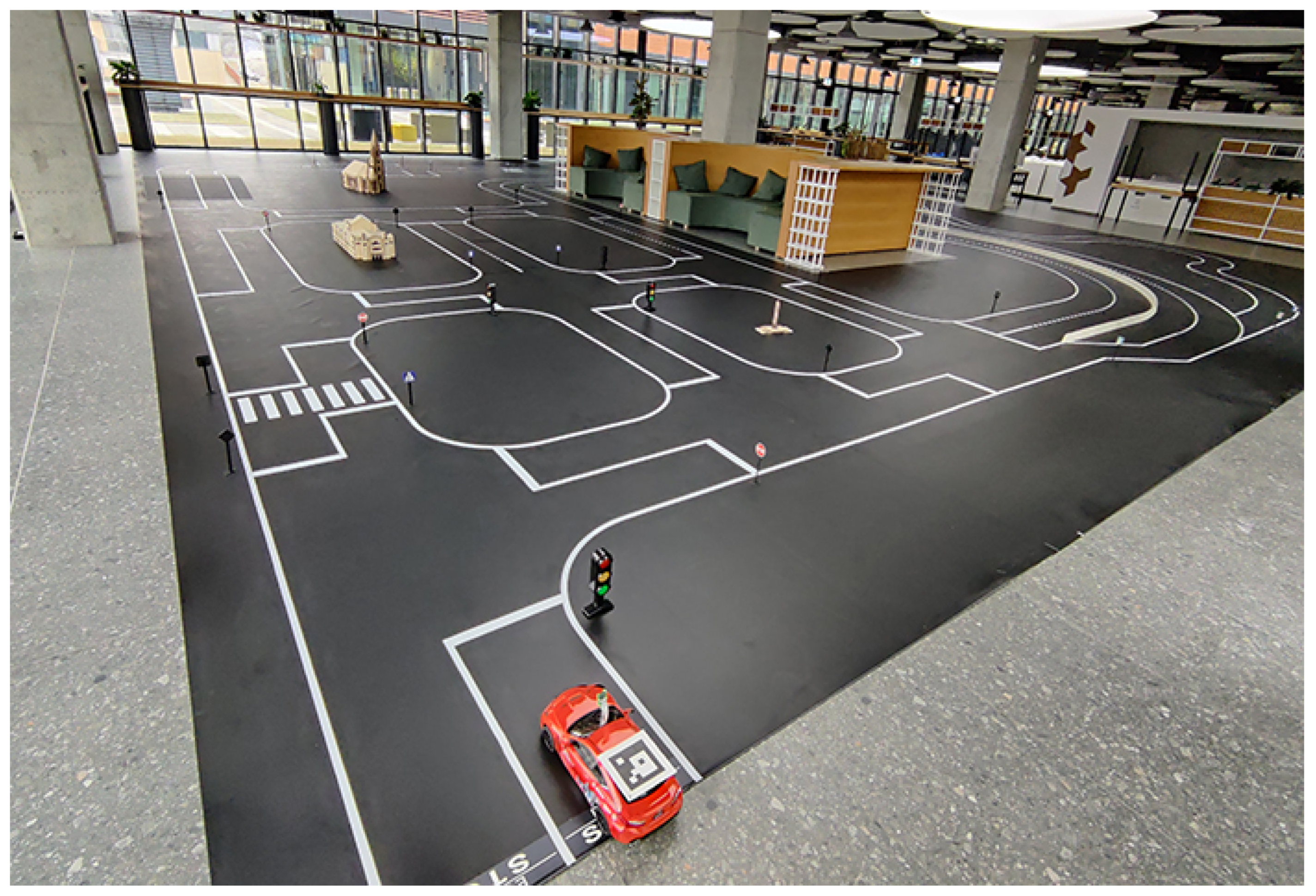
3. The Bosch Future Mobility Challenge Competition

In this section, the BFMC competition is described so as to provide the conceptual basis of our design and implementation decisions. The main objective of the BFMC competition is to develop a 1:10 scale vehicle, using software with optional hardware modifications, capable of autonomously navigating within a miniaturized smart city. The competition track simulates this setting by using a 20 by 14 m area that includes intersections, highways, parking spots, as well as pedestrians and other vehicles (Figure 1).
The vehicle must perform several tasks in real time. It must stay within designated lanes, even where road markings are missing, and recognize traffic lights and signs. It should navigate intersections and roundabouts, and find suitable parking spots to execute parking maneuvers. Giving priority to pedestrians and overtaking other vehicles when appropriate are also required. The vehicle must communicate with its environment, receiving data such as vehicle location or traffic light signals (green, yellow, or red), and publish environmental perception data. While not all tasks contribute directly to points, failure to perform them will result in point deductions. The tasks are divided into mandatory and optional categories. A failure to perform any mandatory task results in halving the points earned from optional tasks. The scoring assignment is evident in Table 1 and Table 2.
These tasks are evaluated during the Technical Challenge, serving as the main competition event that awards the most points. In addition to the Technical Challenge, several other tasks also contribute to the overall scoring:
  • Project Development: Teams submit monthly status updates showcasing their progress, approach, and future plans. These updates include a written report, a video, and a project timeline.
  • Speed Challenge: This is an additional run where points are awarded only if the vehicle successfully completes a predetermined path within a set time limit.
  • Car Concept: This is an evaluation focusing on several criteria, including the scalability of the vehicle, reconfigurability, and robustness. Another factor is the hardware-to-software ratio, examining how well the vehicle performs given its hardware. Teams present these aspects before their runs, highlighting the strengths of their designs.
  • Run Evaluation: Points are given based on the vehicle’s overall performance, considering the experience from both a hypothetical passenger’s perspective and that of a pedestrian observing the vehicle.
It is important to note that the described point system applies solely during the semi-finals and finals. To qualify for the semi-finals, teams have to submit a video proving their vehicle’s ability to perform lane-keeping, navigate intersections, and response to key traffic signs, such as stop, crosswalk, priority, and parking.
The competition provides a starting kit to all participating teams, allowing them to focus on developing their algorithms, rather than creating a hardware solution. Teams are permitted to modify or completely change the hardware, provided that they keep the original chassis and the total cost of these modifications does not exceed the amount of EUR 1000. The kit includes the basic car chassis, equipped with a brushless DC motor with an integrated encoder, as well as a servo motor that handles the steering wheel. The power management is performed via a power distribution board with an integrated power sensor (development board provided by BOSCH Engineering Center), and the car is powered by a two-cell lithium-polymer (LiPo) battery with a capacity of 5500 mAh. The computational unit is a Raspberry Pi 4, 8GB, and the provided sensors are a wide-angle PiCamera V3 and the BNO-055 IMU. Finally, the Nucleo F401RE board is used as the connector between the computational unit, the sensors, and the car’s effectors. The provision of this basic kit ensures that each team has the basic, necessary components to operate the car, perceive the environment, and showcase their solutions.

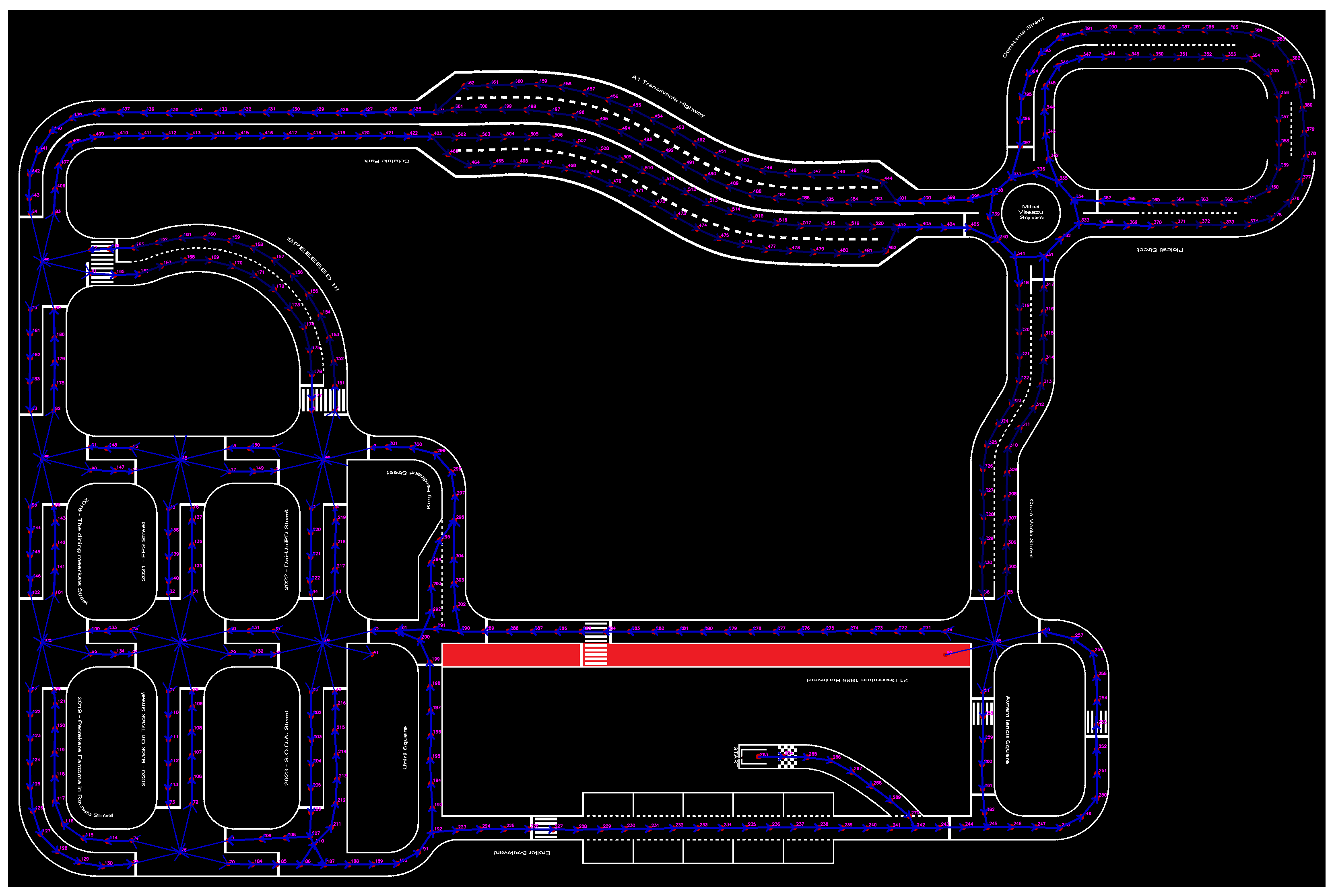
3.1. Competition Requirements

In the 2024 edition of the BFMC competition, the vehicle is required to autonomously navigate through a miniaturized city, completing a series of tasks within a maximum time limit of 10 min. Additionally, it must perform a speedrun challenge, where the vehicle will follow a predefined, long route on an empty track (free of other vehicles, pedestrians, traffic signs, and traffic lights) at its highest possible speed, aiming to complete the course within a maximum of 3 min. All tasks must be executed autonomously, without any external intervention throughout the entire run, and without relying on external processing units. The only permitted user action is the emergency stop, which terminates the vehicle’s navigation process. In terms of energy efficiency, the vehicle is required to operate fully autonomously for at least 30 min on a single battery charge.
To support its navigation, the vehicle must connect to a specific server that provides localization data with a maximum latency of 500 ms. At the same time, the vehicle should publish to this server data about the detected objects and their current speed to be monitored by the jury team. Finally, the vehicle must be able to receive smart traffic light information from the corresponding server via the User Datagram Protocol (UDP).

3.2. Team Requirements

Apart from the competition’s requirements, internal requirements are set as well. Extensive testing helps determine these values as optimal for completing tasks efficiently while minimizing the risk of errors or penalties. For the first part of the competition, the vehicle’s speed must be maintained between 15 and 30 cm/s, with an average target speed of approximately 25 cm/s. These mid-range values prioritize accuracy and stability during task execution, as the focus is more on precision than speed. In the speedrun section, however, the vehicle needs to operate at higher speeds, maintaining a range of 20–45 cm/s with an average of around 30 cm/s. These values approach the vehicle’s maximum speed capacity of 50 cm/s, reflecting the task’s emphasis on speed over accuracy. In terms of system responsiveness, the minimum acceptable iteration frequency for all algorithms for the first part of the competition is set at 10 Hz, whereas for the speedrun, the frequency is increased to 20 Hz to accommodate the increased speed. Additionally, the vehicle must transmit real-time monitoring data—including its status, detected objects, and position on the map—via an MQTT server [26] broker hosted on its main board. The publication latency for this data should not exceed 100 ms. This limit ensures that the user receives timely and accurate feedback, crucial for monitoring and debugging during the vehicle’s technical run.

4. Implementation

Implementing our autonomous vehicle system involves a comprehensive integration of hardware and software components to ensure optimal performance and scalability. This section provides a detailed overview of the hardware design, including the key components and their integration into the vehicle’s structure. We then explore the software architecture, focusing on the system’s modularity, reconfigurability, and the core processes governing the vehicle’s autonomous operations. The logic implementation subsection delves into the decision-making algorithms and control strategies that ensure real-time responsiveness. Furthermore, we describe the software modules responsible for various autonomous tasks and how these modules work together to achieve efficient task execution. Finally, we discuss the real-time monitoring system, which allows for continuous visual feedback to the team and ensures smooth operation and debugging throughout the system’s deployment.

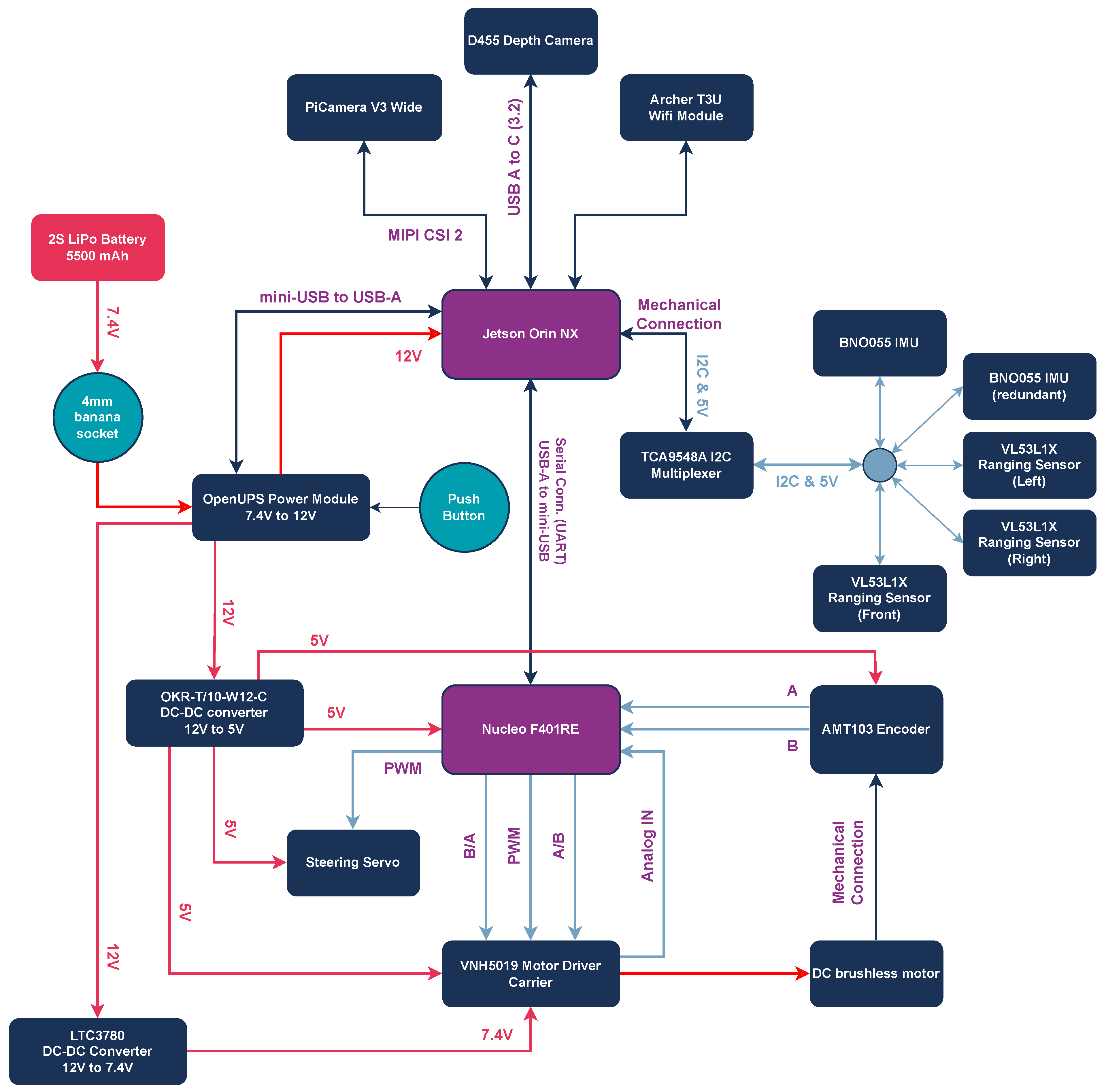
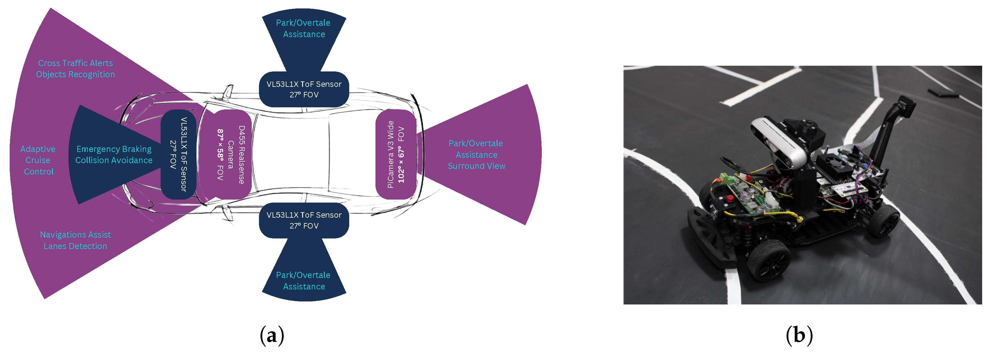
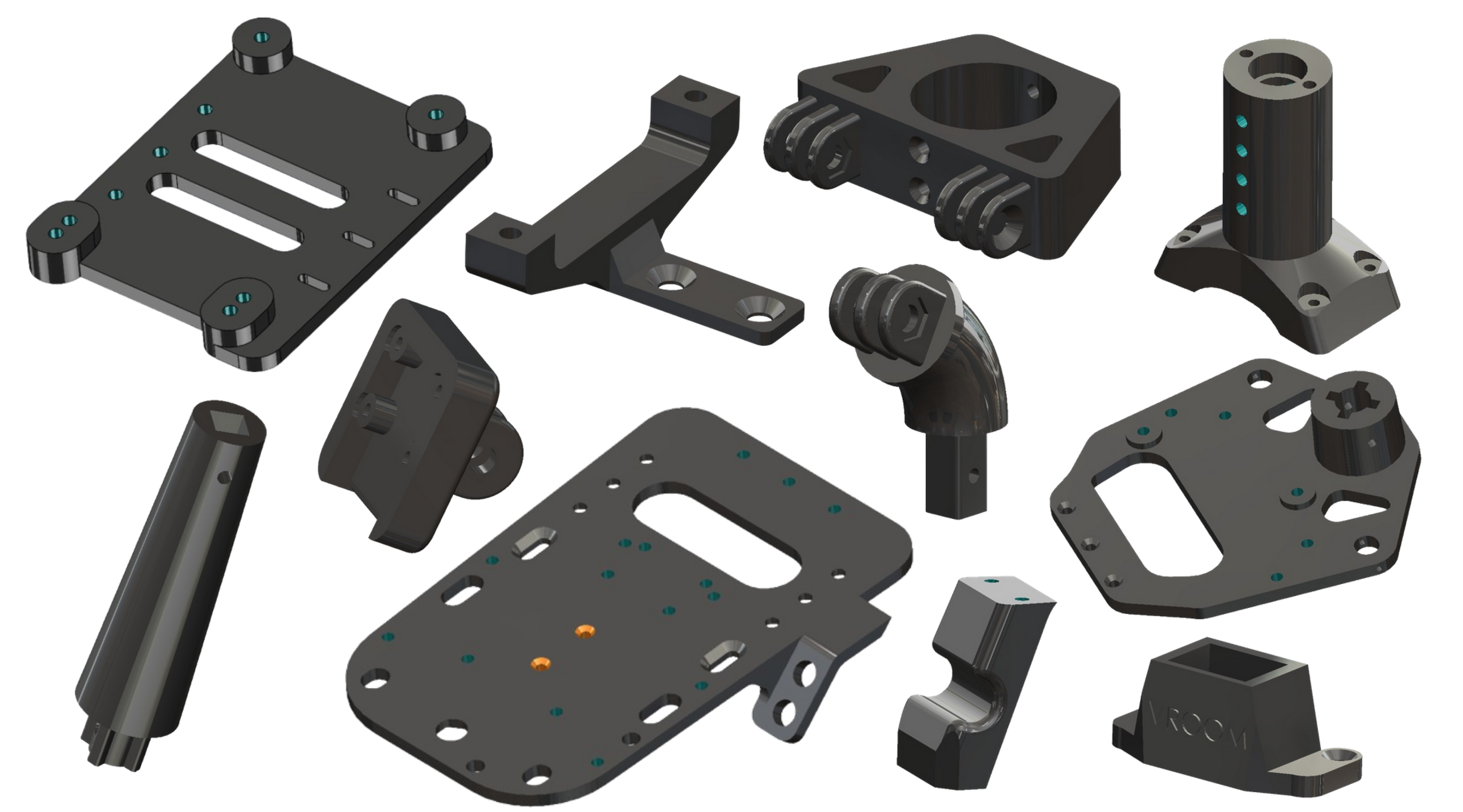
4.1. Hardware Design and Implementation

To ensure a robust and reliable operation, an autonomous vehicle must be able to process large volumes of data in real time, while making accurate and swift decisions based on sensor inputs. A critical aspect of this is the vehicle’s computational resources, which must support complex algorithms for tasks such as sensor fusion, perception, localization, and control. Additionally, robust power management is essential to prevent system failures, ensuring that the sensors, motors, and processing units can operate for extended periods without interruption. These components need to be well-integrated, reducing latency and ensuring that all subsystems work in harmony for seamless operation.
Given these requirements, specific hardware upgrades were implemented to the initially provided competition kit. The Jetson Orin NX 16GB platform (https://www.nvidia.com/en-us/autonomous-machines/embedded-systems/jetson-orin/, accessed on 9 June 2025) is selected over the Raspberry Pi 4 due to its superior computational power, particularly its ability to handle machine learning tasks in real-time. Also, to ensure efficient power usage, the OpenUPS Power Distribution Module (https://www.mini-box.com/OpenUPS, accessed on 9 June 2025) is integrated, offering advanced real-time monitoring and efficient energy management.
In terms of sensors, the vehicle requires enhanced environmental sensing and object detection, as well as classification capabilities for obstacles, other vehicles, pedestrians, and traffic signals. To achieve this, high-precision sensors, such as depth cameras, ranging sensors, LiDARs, or Radars, are typically used to continuously monitor the vehicle’s surroundings. However, given the reduced number of 3D obstacles on the competition track and the high cost associated with LiDAR sensors, we opted not to include them in the current design. Instead, the Intel RealSense D455 (https://www.intelrealsense.com/depth-camera-d455/, accessed on 9 June 2025) depth camera is selected, which provides both depth and color camera streams. The depth stream allows for the accurate extraction of 3D objects in the vehicle’s front field of view, while the color stream, in combination with the PiCamera V3 (https://www.raspberrypi.com/products/camera-module-3/, accessed on 9 June 2025) positioned at the rear of the vehicle, enables robust obstacle classification from both the front and rear. This sensor setup offers an effective and cost-efficient alternative for our vehicle’s perception system, ensuring detection and classification capabilities without the need for LiDARs. A redundant BNO-055 IMU (https://www.bosch-sensortec.com/products/smart-sensor-systems/bno055/, accessed on 9 June 2025) is added for improved orientation calculation and accurate sensor fusion. For enhanced obstacle detection and support in maneuvers such as parking and overtaking, Time-of-Flight (ToF) VL53L1X Ranging Sensors (https://www.st.com/en/imaging-and-photonics-solutions/vl53l1x.html, accessed on 9 June 2025) are integrated at the front, left, and right of the vehicle. The TCA9548A I2C Multiplexer (MUX) (https://www.ti.com/product/TCA9548A, accessed on 9 June 2025) is also employed to handle multiple sensors sharing the same I2C addresses. Finally, a custom 3D-printed structure is developed to house and efficiently support these components, optimizing both stability and performance. The hardware architecture and connectivity of all electronics are presented in Figure 2, and the upgraded vehicle is presented in Figure 3.
All communication protocols employed on the vehicle are highlighted below:
  • All ranging sensors and IMUs communicate via the I2C protocol through the MUX with the Jetson. The physical connection is achieved with jumper wires, while the MUX fits directly on the 40-pin header of the Jetson Carrier board.
  • The depth camera communicates via the USB 3.2 protocol with the Jetson platform. The physical connection is achieved via a USB-A to USB-C cable.
  • The Nucleo and the OpenUPS board communicate via the USB 2.0 protocol with the Jetson platform (serial). The physical connection is achieved via USB-A to miniUSB-A cables.
  • The PiCamera communicates via the MIPI CSI protocol with the Jetson platform. The physical connection is achieved via a 22-pin Ribbon Flexible Flat Cable (FFC).
Finally, all vehicle supporting parts, except for the electronics and chassis, are designed using the SOLIDWORKS 2023 Design Tool Software [27]. These parts are (a) designed to be compatible with a Fused Filament Fabrication (FFF) 3D printer, with a build volume of 18 × 18 × 18 cm 3 , and (b) engineered to simplify the assembly process using threaded inserts, which reduce weight and enhance the structure’s robustness. Once assembled, the vehicle can be separated into four main sub-assemblies for easy storage by removing just six screws. Some of the designed 3D-printable parts are demonstrated in Figure 4.

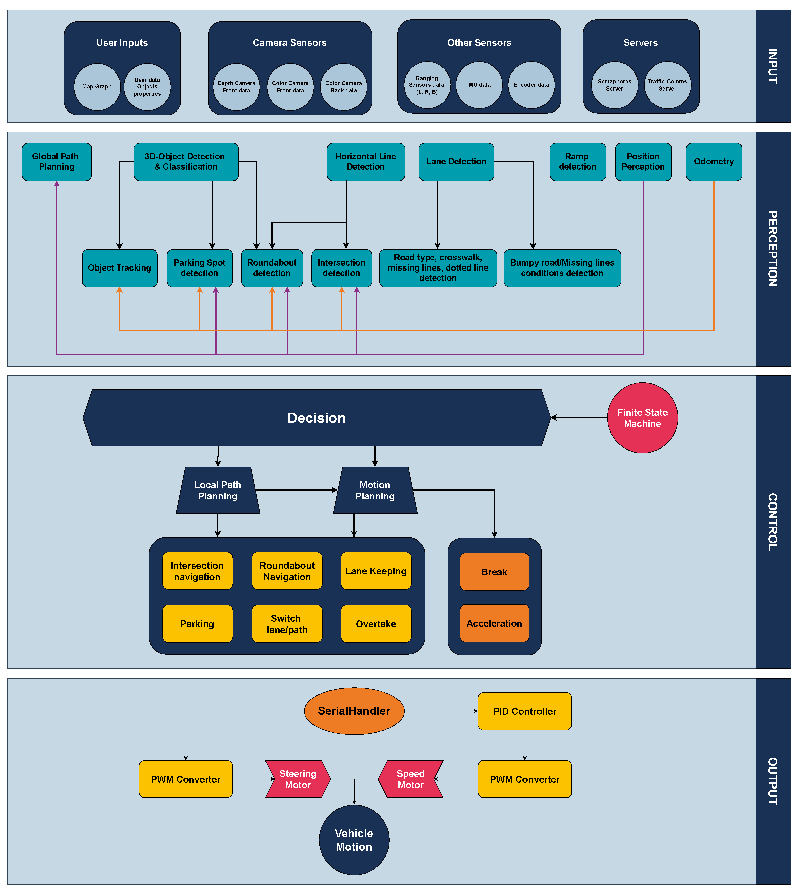
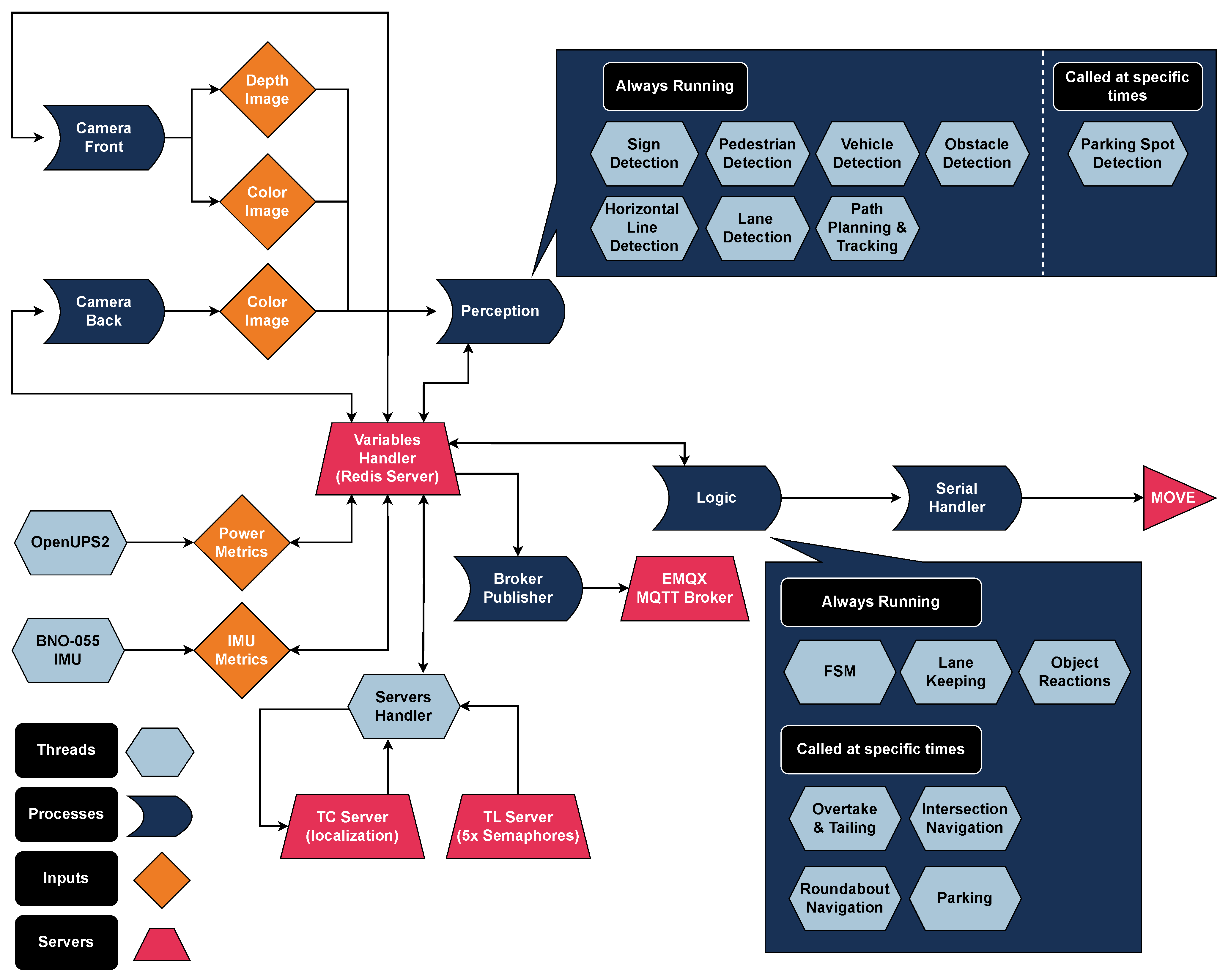
4.2. Software Architecture and Reconfigurability

The software architecture of the vehicle is organized into four primary layers: Input, Perception, Control, and Output. Each of these layers plays a crucial role in ensuring that the vehicle can navigate autonomously by receiving, processing, and acting upon data from its environment. The software architecture diagram, where the four layers are depicted, is presented in Figure 5.

4.2.1. Software Layers

The Input layer is responsible for receiving all sensory data, server information, and the map-graph of the environment. It gathers and preprocesses information from a wide array of sources, including sensors, external servers (for localization and smart traffic light data), and the map, which is essential for defining the vehicle’s navigation path.
In the Perception layer, the system processes all the data collected in the input layer to construct a 3D representation of the environment surrounding the vehicle. This information is then used to make decisions regarding obstacle avoidance, traffic rules, and path planning. Essentially, this layer transforms raw sensor data into actionable insights about the vehicle’s surroundings.
The Control layer is divided into two key components: Action Planning and Behavioral Decision-Making. The perception results, alongside the map graph and path data, are passed through a Finite State Machine (FSM) to determine the appropriate behavior for the vehicle at each time. Once a behavior is selected (e.g., overtaking, stopping, and lane-keeping), the system plans the vehicle’s motion, taking into account the current environment and the planned route. This layer ensures that the vehicle dynamically responds to changing road conditions and challenges.
Finally, the Output layer converts the motion commands from the control layer into the physical movements of the motors. It adjusts the vehicle’s speed and steering using a Proportional–Integral–Derivative (PID) controller to ensure that the desired speed is accurately achieved, while feedback from the encoder data is constantly monitored, allowing the system to make real-time adjustments. The final motion commands, including rotation speed and steering angles, are sent as Pulse Width Modulation (PWM) signals to the brushless motor (for speed) and the servo motor (for steering), respectively.

4.2.2. Asynchronous Functionality

The vehicle’s software architecture is designed with a combination of multiprocessing and multithreading techniques to ensure efficient, parallel execution of tasks. Each of the four primary layers (Input, Perception, Control, and Output) constitutes a separate process, allowing them to operate independently while sharing essential data. Within each process, multiple threads are created to handle the specific tasks required by that layer, thereby maximizing system performance and responsiveness. The decision to use multiple threads within each process stems from the need to concurrently manage various sub-tasks without the overhead of starting and stopping new processes. For instance, in the Perception layer, separate threads handle different sensors, allowing the system to collect data from multiple sources in parallel and process that information in real time. Similarly, in the Control layer, distinct threads handle different aspects of behavior selection, path planning, and motion adjustment to maintain a smooth driving experience. Finally, we opted for a multiprocess architecture, as it offers greater isolation and error handling for each layer. This approach helps ensure that if one process encounters an issue, the others can continue functioning. By segregating the primary responsibilities into processes, we prevent potential bottlenecks that could arise if too many tasks are managed within a single process. This functionality is visually presented in Figure 6.

4.2.3. Data Publishing

In addition to these core processes, an extra MQTT Publishing Process exists, dedicated solely to transmitting vehicle state data, sensor readings, and other vital information to the user interface in real-time. This design isolates the communication layer from the rest of the vehicle’s core functionality, preventing any delays in control or perception processing due to communication overhead.

4.2.4. Inter-Process Communication

The communication between the Input and Perception layers, as well as between Control and Output, is facilitated by duplex pipes (Multiprocessing.Pipe), enabling bidirectional communication with minimal latency. This is critical for maintaining synchronization between the perception of the environment and the physical actions of the vehicle. For the remaining communications—notably between Perception, Control, and Publishing—we utilized a Redis server. Redis was chosen for its speed and lightweight nature, allowing fast storage and retrieval of parameters shared across processes. Each process can efficiently store its data on Redis and access the necessary parameters from other processes, ensuring consistent communication without significant overhead. Redis’ in-memory data storage provides near-instantaneous access to shared data, which is crucial for maintaining the real-time performance of the vehicle’s systems. The combination of processes and threads, along with efficient communication mechanisms like pipes and Redis, ensures that the system can handle a wide range of computational tasks concurrently while maintaining the low-latency requirements necessary for autonomous navigation.

4.2.5. Reconfigurability Aspect

It should be stated that the system is designed for flexibility and ease of testing, with all configuration parameters centralized in a single .ini file. This file consolidates the settings related to vehicle states, hardware components, and communication with other environment systems, allowing for the efficient management of these parameters. Enabling or disabling specific features is as simple as editing the .ini file, streamlining the process of adapting the vehicle to different testing conditions. By using this centralized approach, we significantly reduce the risk of errors that can arise from manually editing multiple scripts. In many complex systems, modifying multiple codebases for different test scenarios introduces the possibility of overlooking parameter changes, leading to inconsistent configurations or unintended behaviors. The centralized file ensures that all related parameters are properly synchronized, making the testing process more reliable and error resistant. Furthermore, the system is designed to be easily reconfigurable through a custom-built web-based monitoring application. Instead of manually editing the configuration file or diving into the code, developers and testers can adjust parameters using an intuitive graphical user interface (GUI), presented in Section 4.5. Toggle buttons, selection fields, and other interface elements allow quick changes to configuration settings without needing to directly interact with the underlying code. This not only simplifies the testing and debugging process but also improves usability, especially for teams working collaboratively or for those less familiar with the system’s inner workings. Finally, the GUI provides safeguards by offering predefined value ranges for specific parameters, minimizing the risk of misconfiguration, and ensuring that the vehicle’s behavior remains within safe operational limits. This method enhances the system’s robustness, as each parameter can be accurately adjusted with ease, reducing the setup time and increasing testing efficiency.

4.3. Logic Implementation

The selection of the vehicle’s actions based on the perception results, as previously mentioned, is governed by a Finite State Machine (FSM), which is depicted in Figure 7.
There, it is clear that all FSM states either begin or end in the Lane-Keeping state, as this is designated as the vehicle’s default state. Deviations from this state occur only when specific path flags (e.g., approaching intersections or roundabouts), environmental conditions, or obstacles are present. The system continuously returns to the Lane-Keeping state after completing any higher-priority task or maneuver.
When multiple perception flags are simultaneously triggered, the system follows a predefined priority hierarchy to ensure that the most critical actions are performed first. The priority of execution is structured as follows:
  • Priority 1—Pedestrians: Ensuring the safety of pedestrians is paramount. If a pedestrian is detected within or near the vehicle’s path, the FSM immediately switches to handle this scenario.
  • Priority 2—Vehicles: If another vehicle is detected, the FSM prioritizes managing the situation by determining whether an overtaking maneuver, vehicle tailing, or stopping is required.
  • Priority 3—Traffic Signs/Lights: Obeying traffic signs and lights is crucial for safe navigation, and the FSM shifts states accordingly to manage these.
  • Priority 4—Path Flags: Finally, the FSM handles route-related flags, ensuring proper navigation through complex road elements like intersections.
This hierarchical design ensures that the vehicle can effectively react to multiple environmental stimuli while maintaining a clear, structured decision-making process.

4.4. Software Modules

In this section, we present the core functionalities that enable the vehicle to perform a wide range of autonomous driving tasks. These modules are designed to ensure the vehicle can navigate complex environments and handle various scenarios encountered on the track. Key tasks such as Lane Following provide the capability of maintaining a stable trajectory within designated lanes, while the 3D-Objects Detection and Reaction module allows the vehicle to identify and respond to obstacles in real time. Advanced navigation techniques are incorporated through the Intersection and Roundabout Navigation module, enabling the vehicle to safely traverse complex traffic scenarios, and the Parking Navigation module, which assists the vehicle in executing precise parking maneuvers. Also, the Overtake Procedure module enables the vehicle to handle scenarios where it must safely pass other vehicles, ensuring smooth and efficient movement throughout the track. Finally, Global Path Planning is implemented to ensure the vehicle follows an optimized route from start to finish, adapting dynamically to the environment. These software modules work in harmony, allowing the vehicle to exhibit high levels of autonomy while maintaining safety and robustness.

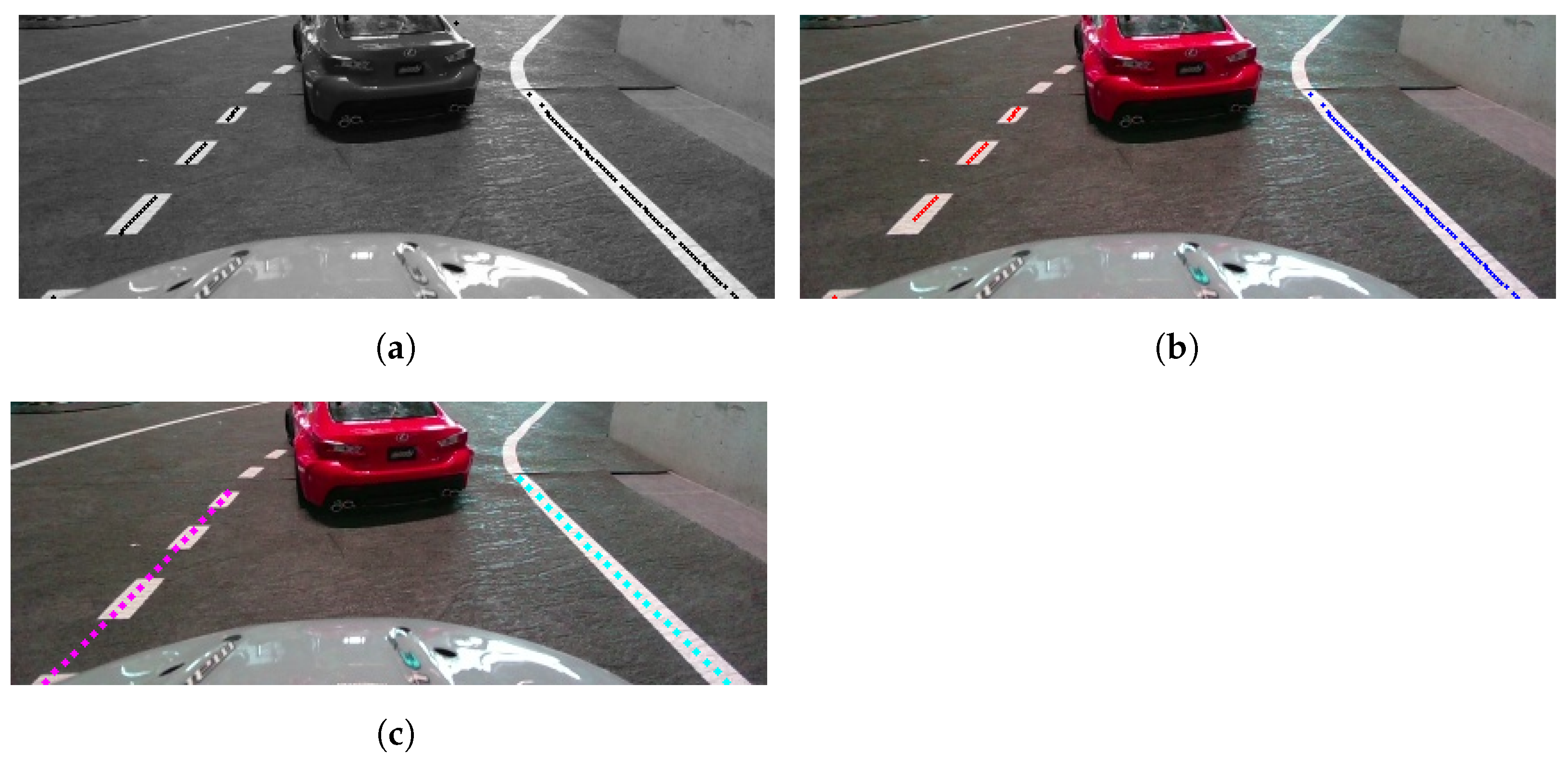
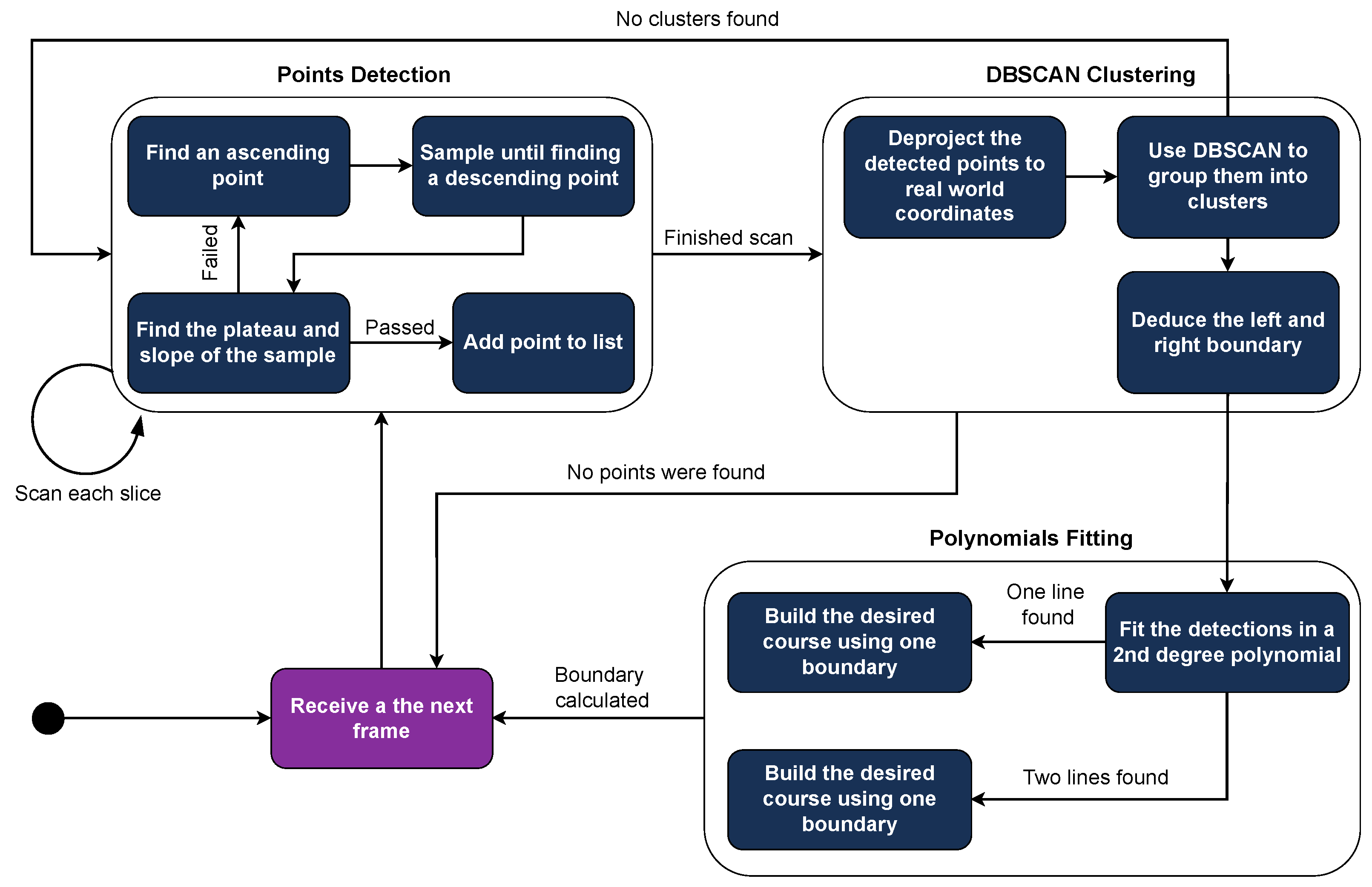
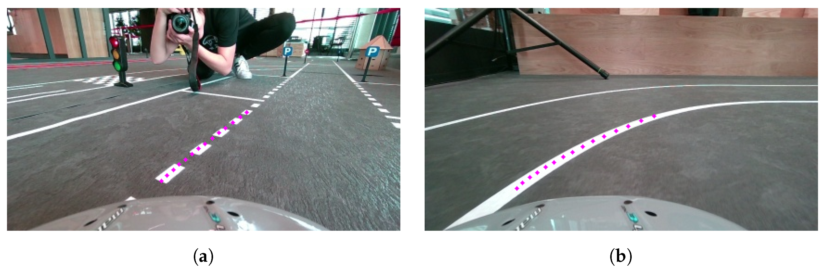
4.4.1. Lane Detection

For detecting the desired lane’s boundaries, we employed a point detection, deprojection, and clustering algorithm. In the initial stage, the image is converted to grayscale and divided into equally sized slices. Each slice is scanned for abrupt changes in pixel values (0–255). When such a change is detected, it is marked as an a s c e n t _ v a l u e , and subsequent pixels are saved in a buffer until another abrupt change is found (Figure 8b). The resulting sample is then evaluated and is either accepted as a potential boundary point or discarded. The sample evaluation process includes four validations:
c o u n t e r l e n ( p i x e l s ) · w i n n i n g _ p e r c e n t a g e
p l a t e a u a s c e n t _ v a l u e a s c e n t _ t o _ p l a t e a u
p i x e l s _ t o _ p l a t e a u m i n _ p i x e l s _ t o _ p l a t e a u
l o w e r _ p i x e l _ l i m i t l e n g t h ( b u f f e r ) u p p e r _ p i x e l _ l i m i t
The first two checks (Figure 8a) ensure that the sample maintains a relatively stable plateau and is a potential edge point. The p l a t e a u of the sample is calculated using a variation of the Boyer–Moore majority vote algorithm [28] and an example can be seen in Figure 8c. In the beginning, the value of p l a t e a u (the winner) is set equal to the value of the first pixel in the buffer. The pixel values are the votes, and the c o u n t e r is changed when the value of the current sample falls into a certain range close to the winner. The range is described by ( 1 c o n f i d e n c e _ i n t e r v a l ) · p l a t e a u p i x e l ( 1 + c o n f i d e n c e _ i n t e r v a l ) · p l a t e a u (compared to the original algorithm where the counter is changed when the current vote is strictly equal to the winner). Thus, Equation (1) checks the validity of the p l a t e a u , meaning that the p l a t e a u and in turn the sample are discarded if the surplus in votes of the winner (the c o u n t e r ) is less than a proportion ( w i n n i n g _ p e r c e n t a g e ) of the sample size. Equation (2) checks if the difference between the highest value in the sample (the p l a t e a u ) and the lowest ( a s c e n t _ v a l u e ) is greater or equal to a s c e n t _ t o _ p l a t e a u , a threshold above which the sample is considered an edge point and in our case a potential boundary point. Equation (3) rejects points that belong to a reflection of light on the track since reflections tend to follow a distribution similar to white noise, and therefore the distance between the a s c e n t _ v a l u e and p l a t e a u is large. Keeping m i n _ p i x e l s _ t o _ p l a t e a u relatively small (this depends on the lighting conditions of the track) eliminates most of the unwanted reflection samples (Figure 8d). This happens since we expect reflections to reach the plateau value in a less sudden and more gradual way. Finally, the last check performed in Equation (4) exists to make sure that the sample is large enough to be part of the road’s boundaries and for the aforementioned checks to produce reliable results. The values of l o w e r _ p i x e l _ l i m i t and u p p e r _ p i x e l _ l i m i t were experimentally defined.
Once all potential boundary points are acquired (Figure 9a), they are deprojected into real-world coordinates using the pinhole camera model in 2D since we only care for points on the track’s surface. The deprojected points are then clustered using the DBSCAN algorithm with finely tuned parameters, separating them into left and right boundary sets based on their position relative to the vehicle’s center (Figure 9b). A set is dropped if the number of points it contains does not exceed a certain value. In cases where multiple left or right sets exist, the set closest to the center is selected for course generation.
For each valid set of points, a second-degree polynomial curve is fitted to reduce the impact of outliers and create a smooth course (Figure 9c). If both boundaries are detected, the desired course is calculated by averaging the two curves. If only one boundary is detected, the course is shaped with the same curvature as that boundary but is padded to align with the vehicle’s center. The internal logic of the Lane Detection software module is illustrated in Figure 10.

4.4.2. Lane Keeping

Regarding the Lane-Keeping algorithm, our approach uses a Pure Pursuit Controller with adjustable gain to control the vehicle’s heading through its steering. The desired_steer results from the following equation:
d e s i r e d _ s t e e r = 90 d e g r e e s ( a t a n ( v e r t i c a l _ g a i n , e r r o r ) )
Here, e r r o r is the horizontal distance between the vehicle’s center and the weighted mean average of all the boundary points in the desired course, and v e r t i c a l _ g a i n is the horizontal coordinate of the bottom point in the desired course multiplied by the appropriate gain.
This type of controller was chosen for its simplicity and computational efficiency. The reason behind the utilization of an adjustable gain was that this type of controller produced the same steering angles for both cases where the vehicle entered a straight road in an off-angle and when it had to take a sharp turn. The result was that in the first scenario (and especially at high speeds), the vehicle abruptly corrected its course (as it should when facing a sharp turn) leading to oscillations, which in turn could force the vehicle to go off track. To avoid this behavior, the gain of the controller was adjusted according to the desired course’s slope, calculated by the lane detection module. If the slope was small, meaning that the road was straight but the vehicle was facing it at an off-angle, it corrected its course more smoothly than if the slope was large, meaning that the vehicle was facing a turn. An example of this can be seen in Figure 11. In this example, when the vehicle is exiting a parking spot, it enters the road in an extreme angle (Figure 11a); therefore, without the desired course slope check and the subsequent gain change it would behave as if it was taking a sharp right turn (Figure 11b).
When a crosswalk is detected, the car should slow down and pass it in a controlled manner, which is implemented with a simple Proportional–Integral (PI) controller. The size and mechanics of our vehicle enabled us to use the bicycle kinematic model to approximate its movement. Since the Lane-Keeping algorithm ensured that the vehicle remained inside the lanes when facing the crosswalk, the controller only needed to account for the correction of the vehicle’s heading ( t a r g e t _ y a w ). The vehicle’s orientation using the bicycle model is calculated using the following formula:
ψ t + 1 = ψ t + V t L f · δ t · d t
Here ψ is the vehicle’s current (t) and next ( t + 1 ) yaw; V t is the vehicle’s current speed, which for the Crosswalk passing remained low and constant; L f is half the vehicle’s length; and δ t is the vehicle’s current steering angle. Say u represents the controller; then the next yaw should be given by the formula
ψ k + 1 = ψ k + u
The general PI controller for discrete applications is described by
u [ k ] = K p · e [ k ] + K i · j = 0 k e [ i ] Δ t
From (6) and (8) can be deduced that the controller’s final form will be
u = K p · ( ψ k ψ k 1 ) K i · ( ψ t a r g e t ψ k ) · ( t e n d t s t a r t )
Finally, since we are interested in the value of the steering angle each step, from (6) and (9) we get
δ k = L f · u V t ( t e n d t s t a r t )

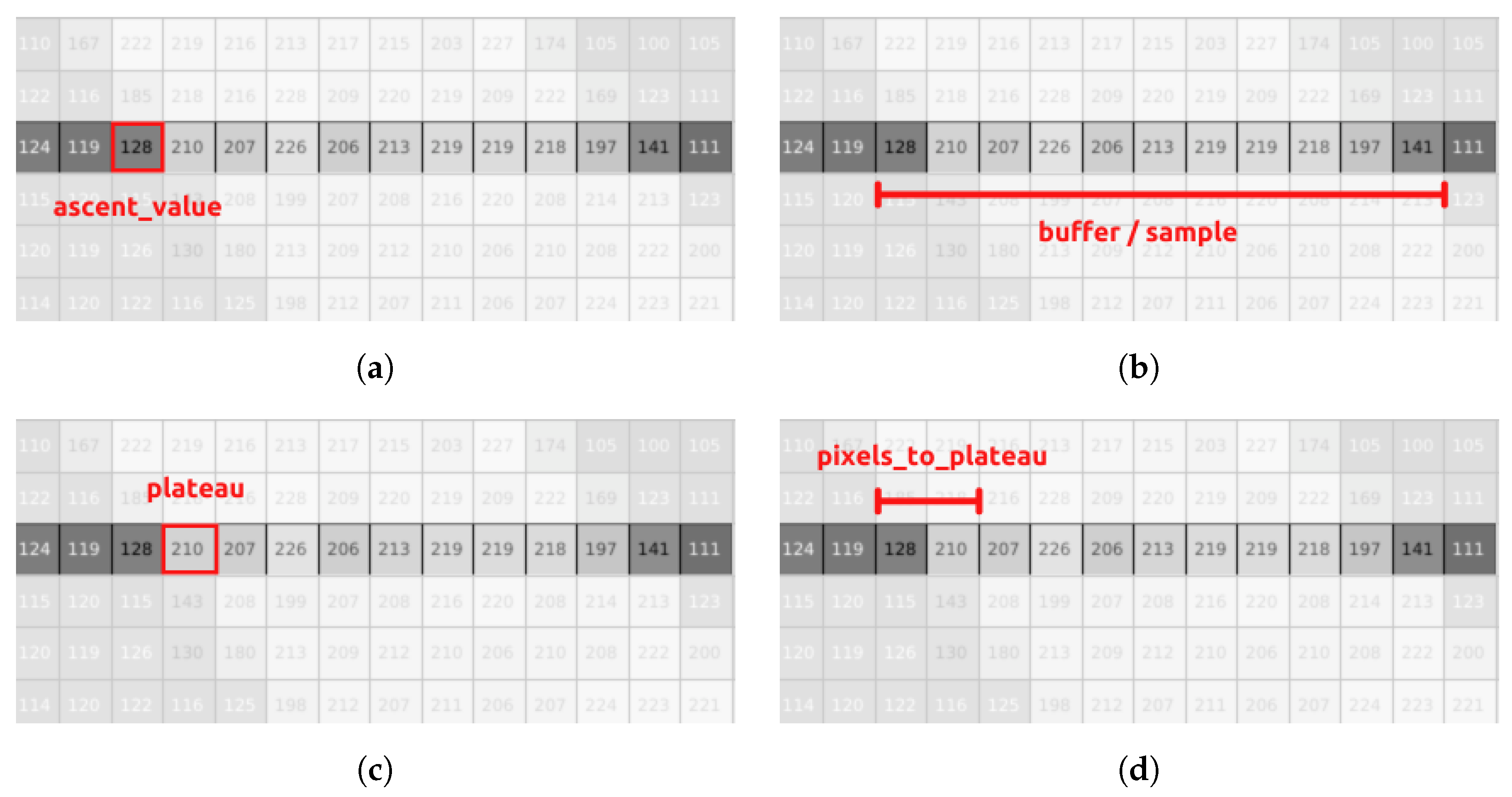
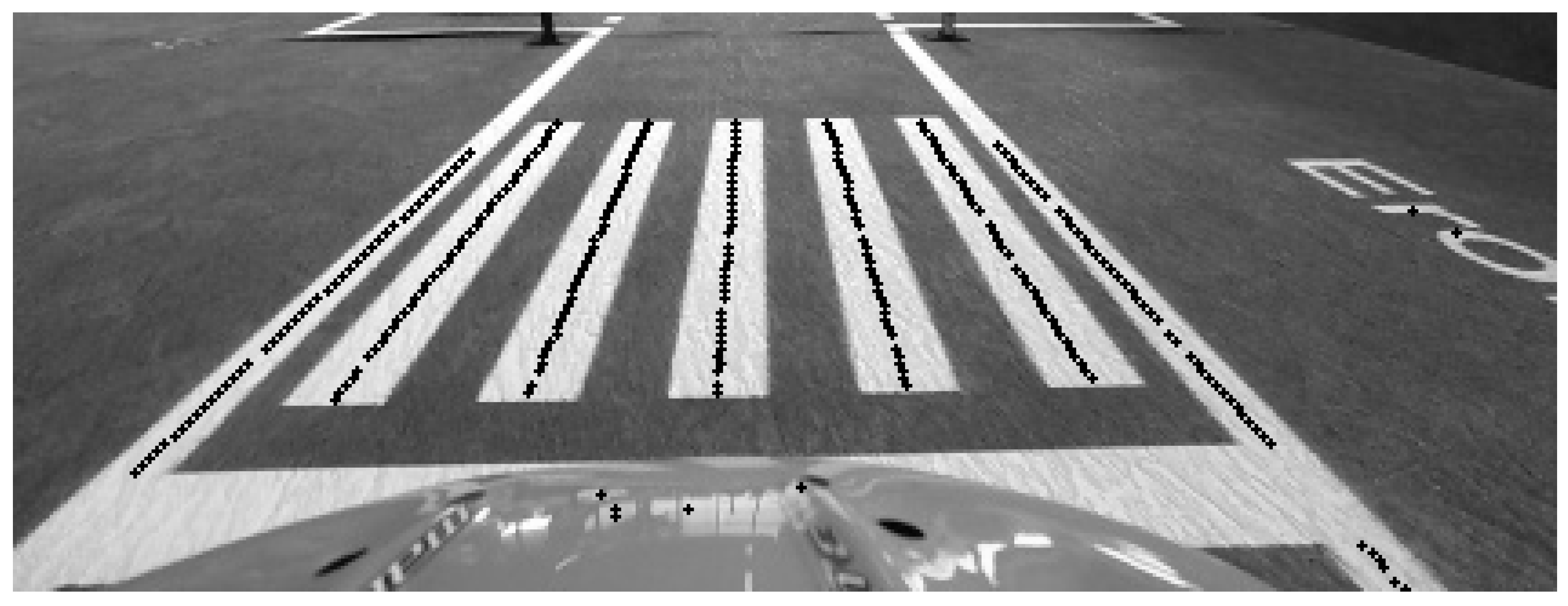
4.4.3. Crosswalk Detection

Using the first two steps of the Lane Detection algorithm, we can also deduce if the vehicle is facing a crosswalk or not. The steps to detect a crosswalk are visualized in Figure 12 and are described below:
  • Finish the points detection phase in the Lane Detection process.
  • For each slice produced, check the number of detected points in it.
  • Calculate the average number of points per slice, and if it is above a certain threshold, a crosswalk is detected.
It is evident that the algorithm relies heavily in the accuracy of the lane detection algorithm. Therefore, the threshold parameter was not set too high because then a crosswalk pattern would be very hard to detect. On the other hand, if set too low, then many sparse patterns (line-wise) would be mistakenly classified as a crosswalk. This algorithm was proven effective mainly because the competition’s track never had any crosswalk lines missing, and therefore the pattern was unique and prominent.

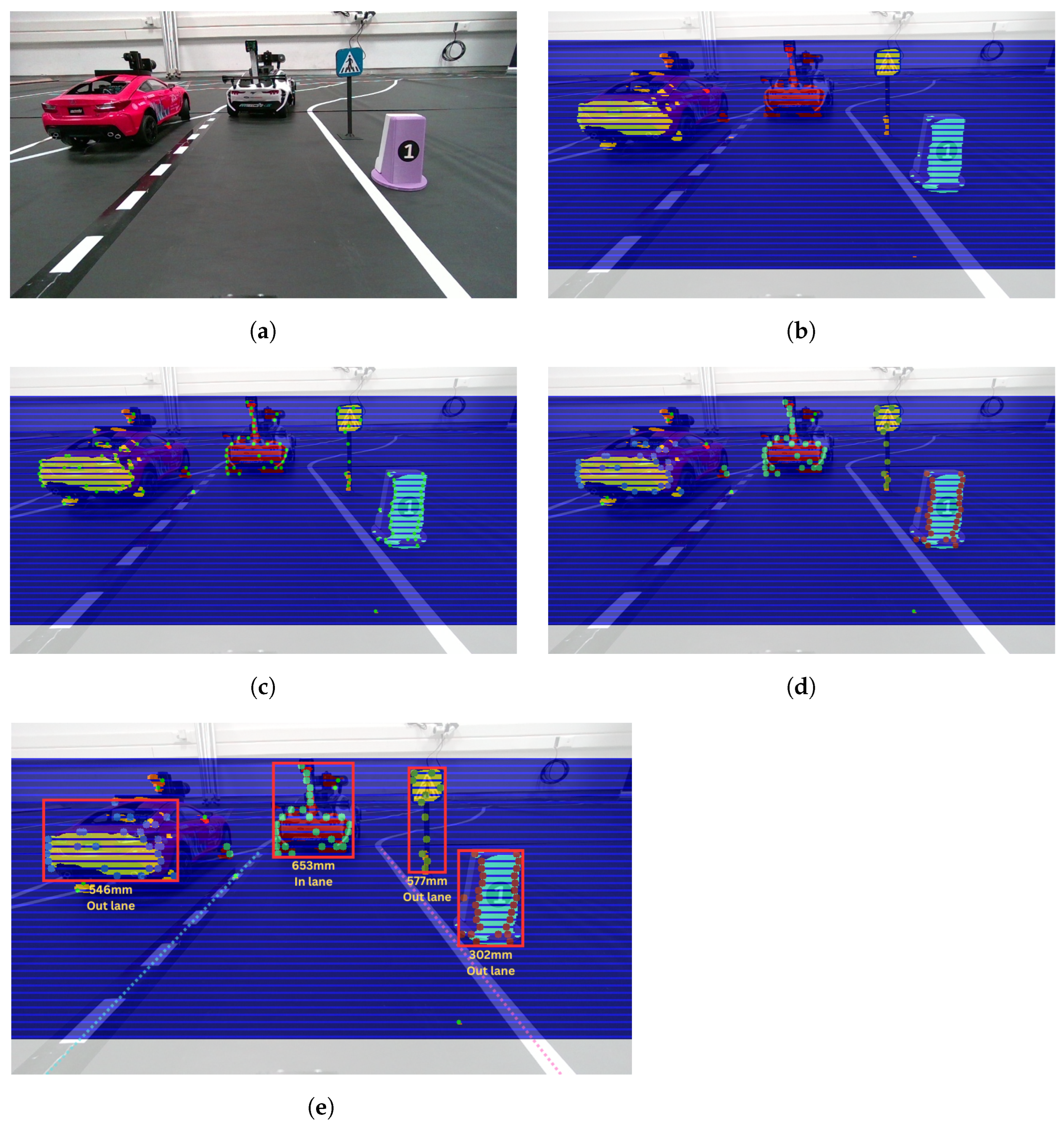
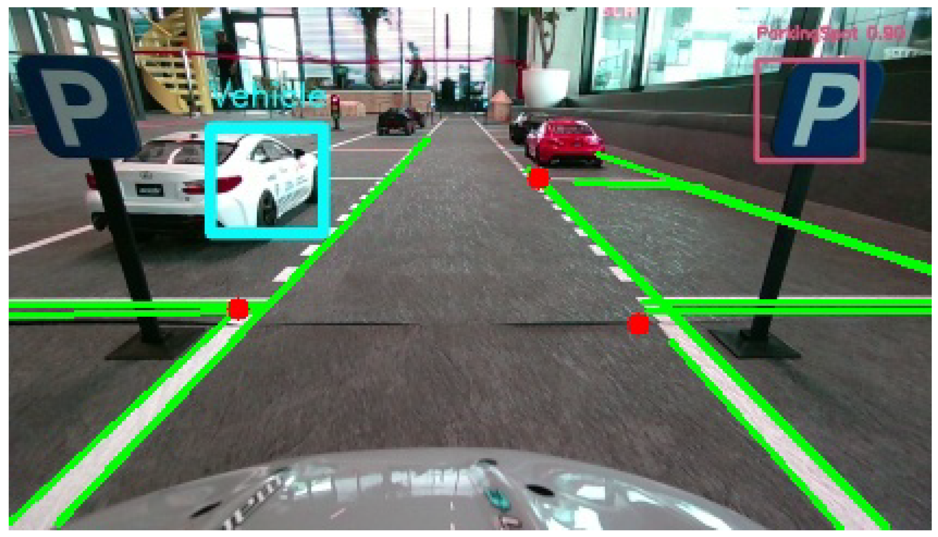
4.4.4. 3D-Objects Reaction

To accurately identify objects within the vehicle’s environment, we utilized depth maps generated by the available depth sensors. An innovative technique was developed, where the depth frame is divided into predefined slices, each treated as an individual signal for peak detection. These detected peaks are subsequently clustered using the DBSCAN algorithm with finely tuned parameters, enabling the precise separation of objects from the background. After clustering, a bounding box is applied to encompass all the peaks within each cluster, and the median distance of the object is calculated based on the individual metrics of each peak.
When an object is detected, before classification, we first estimate whether it is within our lane or outside of it by utilizing the output from lane detection. Specifically, we calculate the pixel coordinates of the center point of the object’s bounding box and assess whether those coordinates fall within the area defined by the lane boundaries in the image. This quick check helps to determine whether the detected object is likely to obstruct the vehicle’s path and requires further processing as a potential obstacle to navigation. The obstacle detection process is visualized in steps in Figure 13.
Initially, we must verify that no immediate action, such as deceleration or stopping, is required. To achieve this, two distance thresholds are dynamically adapted relative to the vehicle’s speed. If the detected object is within the lane and its distance falls between these thresholds, the vehicle decelerates. If the distance is below the lower threshold, the vehicle stops to ensure that the object can safely cross the road. Finally, if the object does not move, the vehicle will perform the appropriate maneuver after replanning its route.
After detection, the object is classified into one of the following categories: vehicle, pedestrian, traffic sign, traffic light, or obstacle. For this purpose, we employ the following machine learning models:
  • YOLOv9-c introduced by Wang and Liao [29] for Traffic Sign and Traffic Light classification. This model is trained on a custom-made dataset consisting of approximately 10,000 images per class, with annotations performed in-house.
  • Semantic Segmentation with a ResNet-18 backbone, trained on the Cityscapes dataset, for the classification of vehicles, trucks, and buses.
  • Body Pose Estimation with a ResNet-18 backbone proposed by Bao et al. [30] for Pedestrian classification.
All trained models are exported as .onnx files and subsequently converted to .trt format on the vehicle’s onboard system to ensure optimal performance on the Jetson platform, utilizing specific versions of CUDA and TensorRT libraries. The current models are trained and deployed on the Jetson Orin NX 16GB platform, using CUDA v11.4 and TensorRT v10.1.
Subsequently, the classification results guide the vehicle’s actions:
  • Traffic Sign: The vehicle adheres to traffic rules and responds accordingly (e.g., stopping at a STOP sign, reducing speed at a crosswalk).
  • Traffic Light: The vehicle receives the state of the detected traffic light from the traffic lights server and acts accordingly.
  • Pedestrian: If a pedestrian is within the lane, the algorithm treats it as an obstacle, causing the vehicle to decelerate or stop according to the aforementioned thresholds. If a pedestrian is outside the lane but approaching a crosswalk ahead, the vehicle stops to allow the pedestrian to cross.
  • Vehicle: If the lane on the left is dotted and the vehicle’s speed exceeds that of the vehicle ahead, an overtaking maneuver is initiated. Otherwise, the vehicle follows without further action. Vehicles in other lanes provide information for other parts of the code (e.g., parking navigation) but do not trigger an immediate response.
The agent’s top priority is to ensure the safety of pedestrians and its own passengers. Therefore, stopping is always prioritized in all the scenarios described above. To minimize unnecessary reactions caused by noisy detections, the system employs a majority voting scheme. Specifically, the agent requires an object to be detected at least n times within m consecutive detection loops before initiating a reaction. The detection process has a latency ranging between 50 ms and 100 ms, translating to a frame processing rate of 10 to 20 frames per second (FPS). After extensive testing, the optimal values for n and m were determined to be 4 and 6, respectively. This means that the vehicle must detect the obstacle for at least 0.3 ± 0.1 s, depending on the algorithm’s latency, before reacting. This approach reduces false positives, ensuring the vehicle only reacts to consistently detected objects.

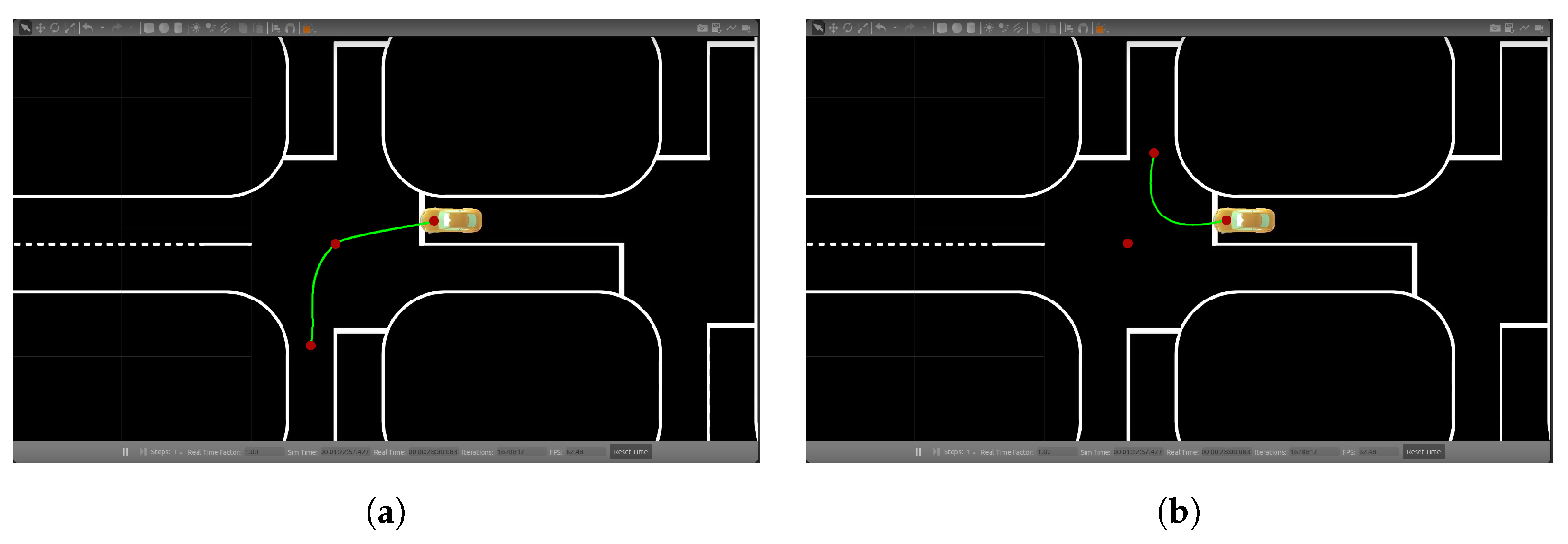
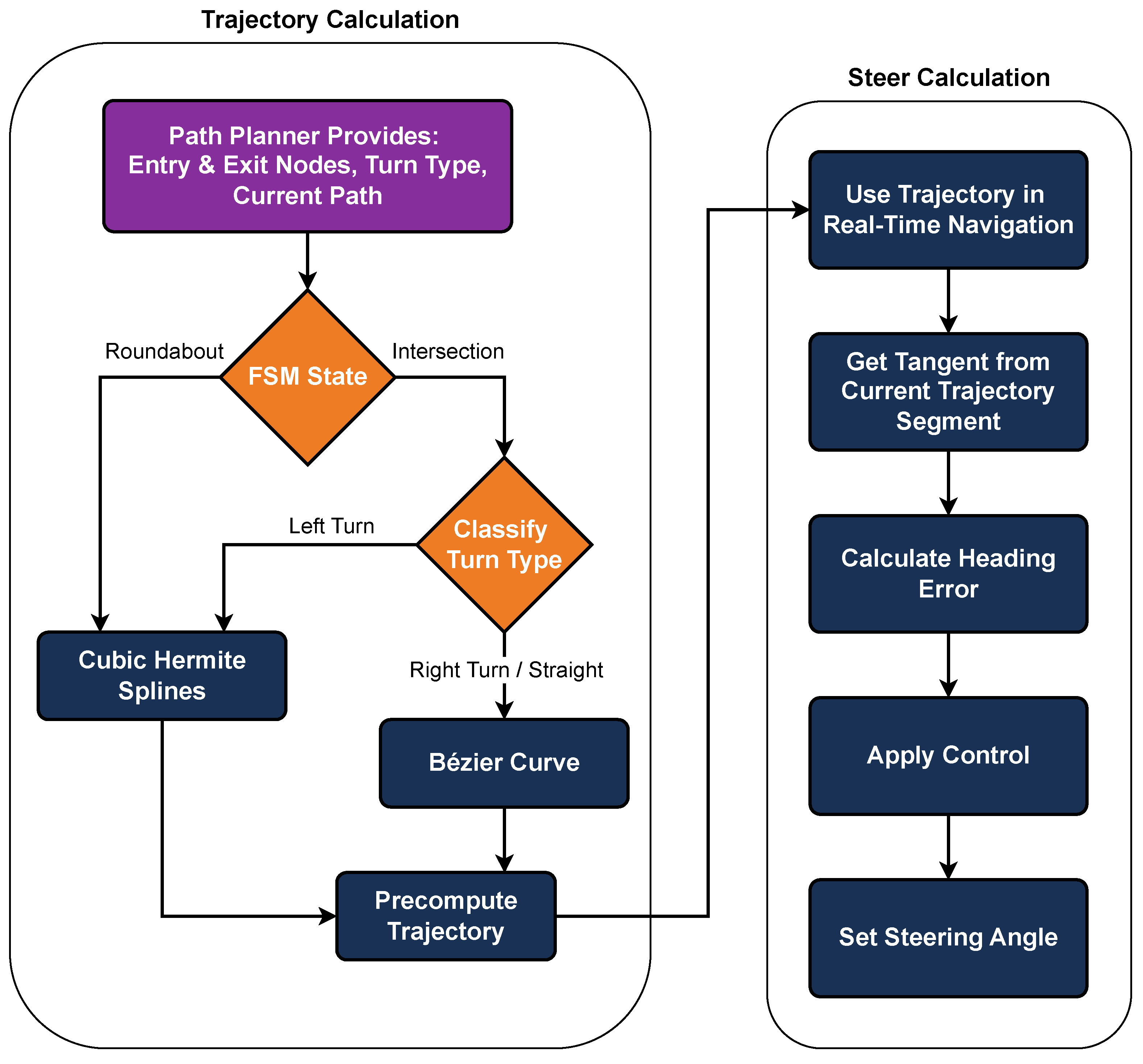
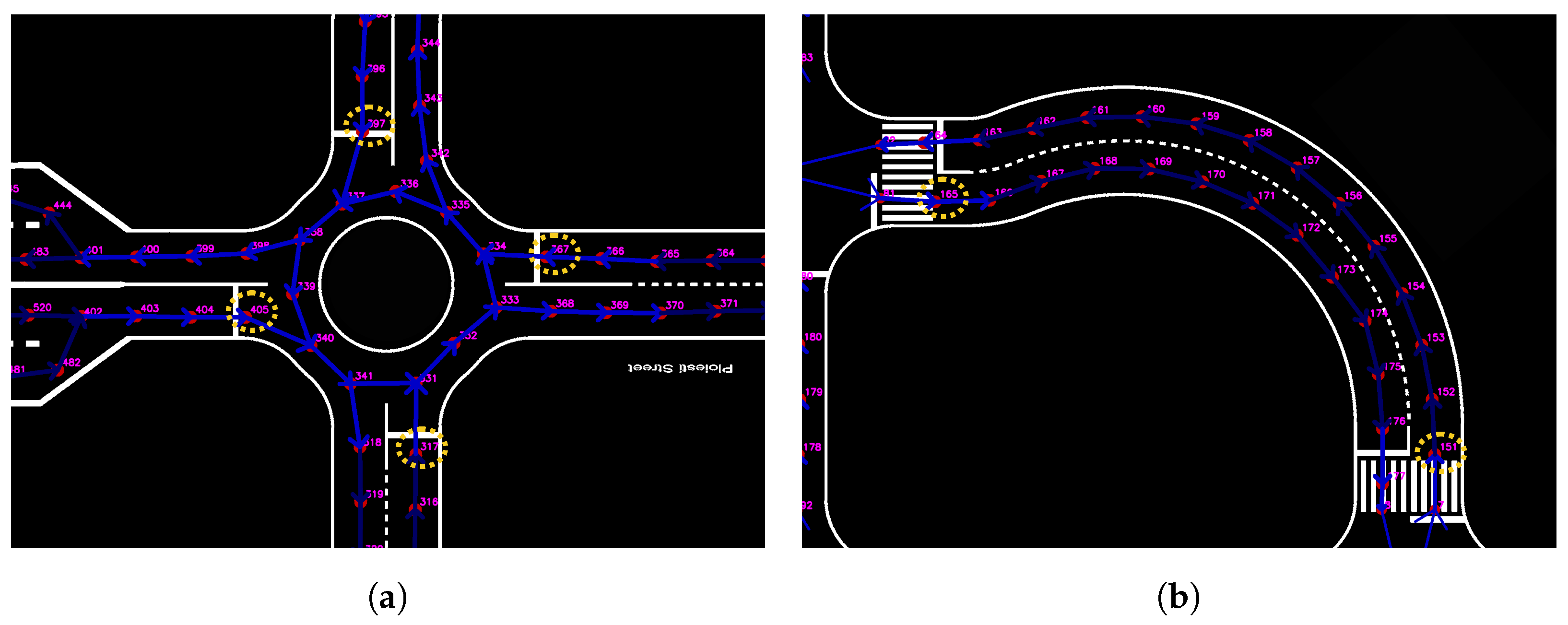
4.4.5. Intersection and Roundabout Navigation

The first step in navigating intersections is to determine what type of turn the vehicle needs to make. The competition map, which is given in the form of a directed graph, can be used to detect the entry and exit points of the intersection. By calculating the absolute slopes between these points, the system can decide whether the vehicle should turn left, turn right, or continue straight. After identifying the turn type, the next task is to generate the vehicle’s trajectory. The techniques of Cubic Hermite Splines and Bezier curves are used for this, as they produce smooth, continuous paths, as is evident in Figure 14a,b. Precomputing the trajectory ahead of time allows for the more efficient use of resources during real-time navigation.
For steering, a tangent point system is applied. This method calculates the tangent of the pre-planned path and compares it with the vehicle’s current direction, implementing a simple D controller. The necessary steering angle is then determined to keep the vehicle on course. This approach works well for simple turns but can be less effective on complex routes that involve multiple changes in direction or more intricate maneuvers. The implementation flow for handling intersections and roundabouts is illustrated in Figure 15.

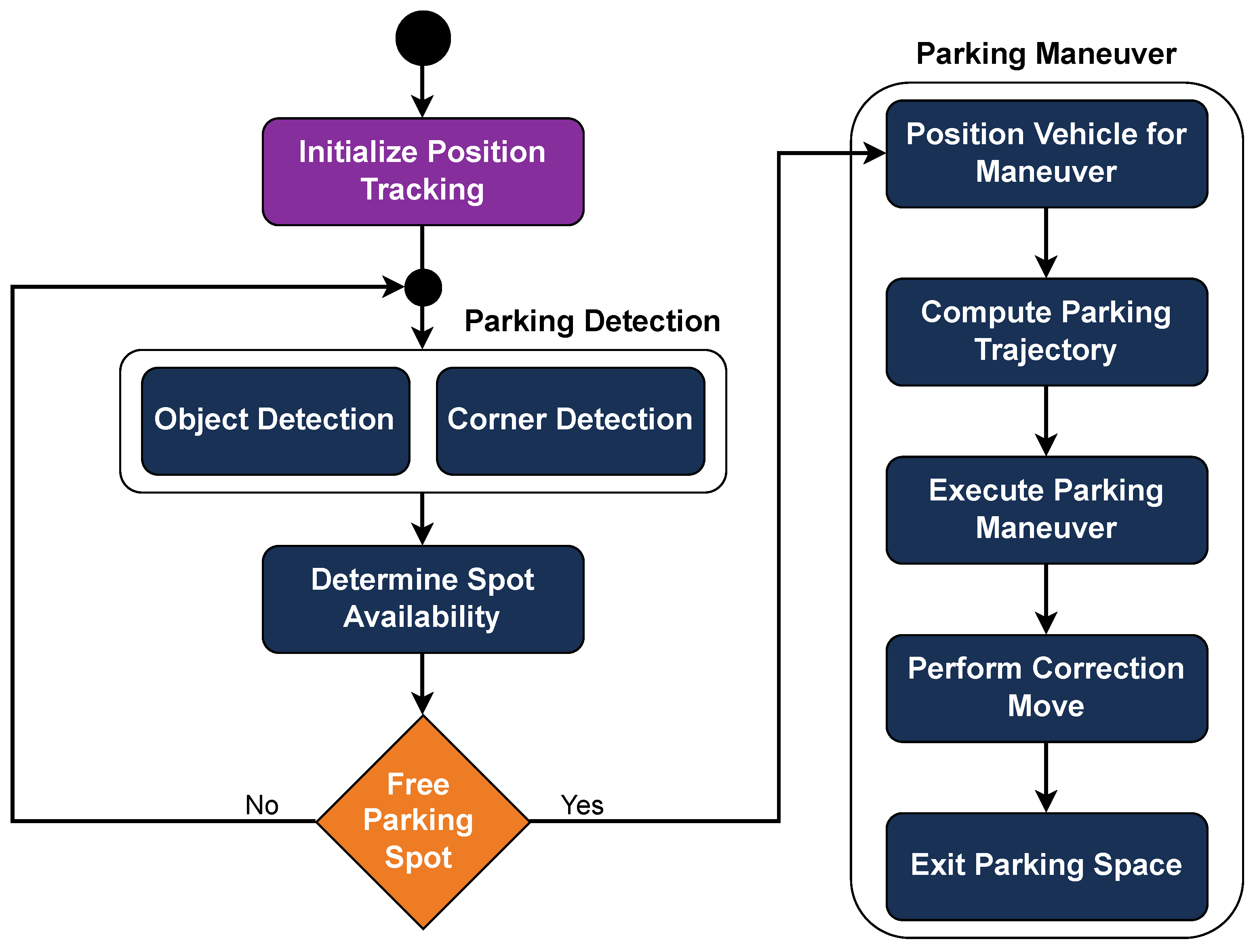
4.4.6. Parking Navigation

In the context of the BFMC, the task of parking involves navigating a designated parking area with a parking sign at the beginning, followed by a number of parallel parking spots. Some of these spots are occupied by other cars, while others are free. The objective is to park in a free space and exit without any collisions.
The parking spot detection process is initiated as soon as the vehicle identifies the parking spot sign. Upon detecting the sign, the car begins tracking its position via odometry to determine the distance traveled from the starting point. To assess the availability of parking spaces, our object detection algorithm continuously scans for nearby parked cars, calculating their locations relative to the starting point of odometry. Simultaneously, a corner detection algorithm, based on Hough lines, identifies the corners formed by the horizontal road markings of each parking space and the road lines, defining the boundaries of the parking spot. The positions of these corners are also calculated relative to the starting point (the position coordinates of both the vehicles and the corners are transformed from image coordinates to real-world ones, relative to the starting point of the odometry). By combining these detections, the system is able to determine which slots are occupied and which are free (Figure 16).
Once a free parking space is detected, the vehicle positions itself in an initial location, at half the length of the parking space ahead, to start the parking maneuver. The parking trajectory is computed using a Quintic Polynomial Planner [31], which generates a smooth and feasible path, and the car follows this planned trajectory using the bicycle kinematic model (Figure 17). After the initial parking maneuver, a single correction move is executed, relying on the horizontal line of the parking space in front as a reference for the car’s alignment. To exit the parking space, the car follows the previously calculated trajectory in reverse. This method allows for precise parking and maneuvering within the challenge’s constraints. The sequential logic of the Parking module is illustrated in Figure 18.

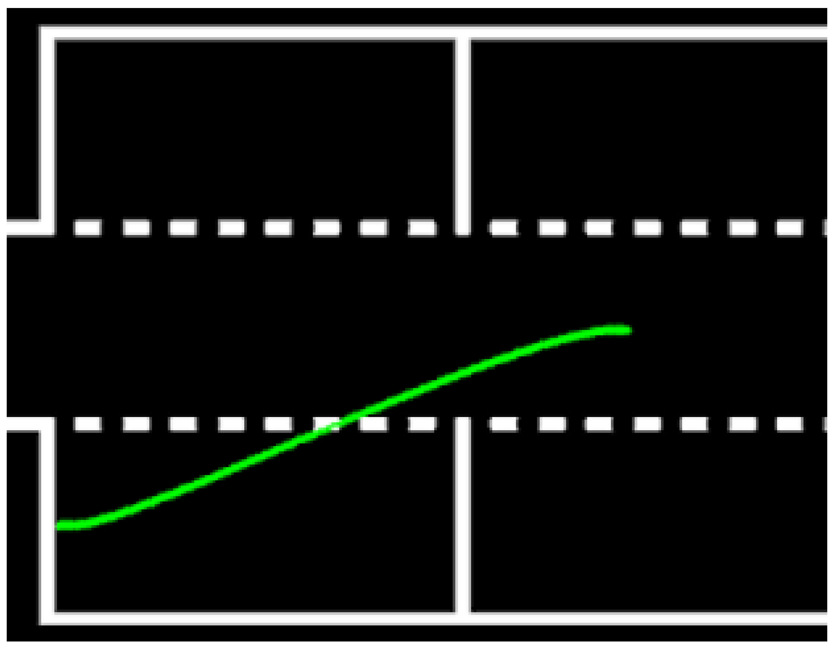
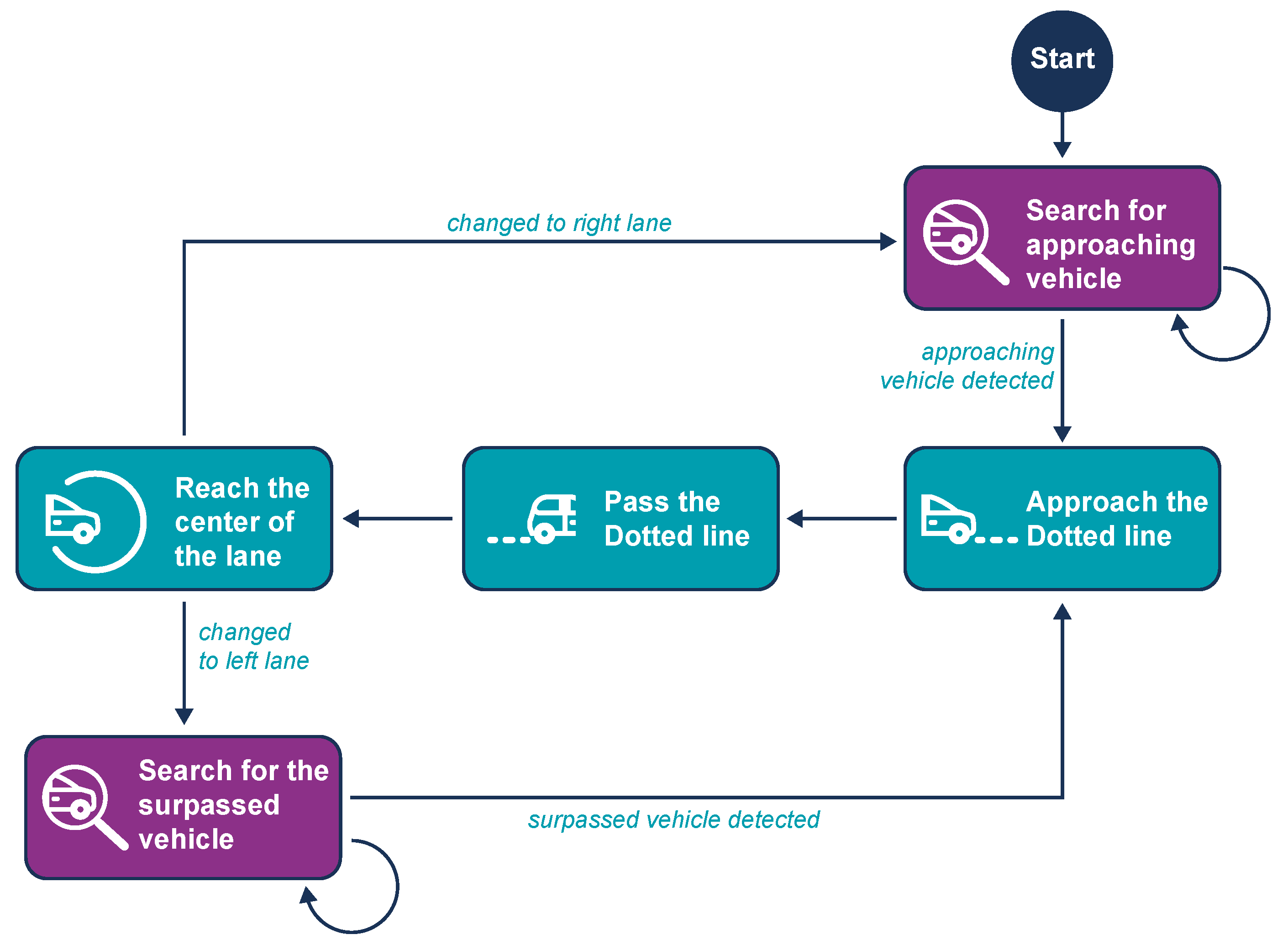
4.4.7. Overtake Procedure

The Overtake process executes a loop that monitors if the distance to any object in the vehicle’s lane decreases, indicating that the object is either stationary or moving slower than the vehicle. If the object is not a pedestrian and there is a dotted line on the left, the Overtake maneuver is initiated. This maneuver consists of three phases: changing to the left lane, driving in that lane until the object is surpassed, and then returning to the right lane.
The Change Lane maneuver itself has three distinct phases. To initiate a left lane change, a negative steering angle is applied, guiding the vehicle toward the left boundary (the dotted line). Throughout the maneuver, the steering is controlled by the Change Lane process, overriding the Lane-Keeping algorithm. However, the Lane-Keeping algorithm continues to calculate steering angles, serving as a reference for the phase transitions. In the first phase, the Lane-Keeping algorithm gradually suggests increasing positive steering angles as the vehicle nears the left boundary. Once these angles surpass a threshold, the vehicle reaches the boundary between lanes, concluding the first phase and initiating the second (Figure 19b). During the second phase, the vehicle crosses the dotted line into the adjacent lane. This phase ends when the Lane Detection system identifies the dotted line as the new right boundary (Figure 19c). At this point, the controller starts suggesting decreasing negative steering angles, as the vehicle is now on the right edge of the new lane and needs to move toward the center. In the third phase, the vehicle nears the center of the new lane, with the steering angles approaching zero or becoming slightly positive (Figure 19d). At this stage, control is handed back to the Lane-Keeping algorithm. While driving in the left lane, the rear camera is activated, and Vehicle Detection runs to monitor the overtaken vehicle. If the overtaken vehicle is detected at a safe distance behind, the final lane change back to the right is initiated, with the same steps as before but in reverse. Once completed, the vehicle returns to the Lane-Keeping state. The overtake procedure is presented as well in Figure 20.

4.4.8. Global Path Planning

The vehicle navigates along a track mapped as a directional graph, provided as a graphml file, including nodes with their corresponding X and Y coordinates and unique I D , as well as edges that define the connections between source and target nodes. Additionally, the graph includes information on whether an edge is dotted or solid. Using this graph, the vehicle must establish its full path at the beginning of the run since it is a prerequisite to visit specific areas related to tasks. This enables it to make navigation decisions at intersections and roundabouts, follow the path throughout the run, and update it if replanning is necessary.
The vehicle begins from a random position on the map, requiring it to determine the source node for its journey. The target node is set as the source node, meaning the vehicle needs to return to its starting position after completing the required challenges. The source node is determined by integrating localization and orientation data. Localization data identifies the lane where the vehicle is positioned, while orientation data indicates the direction of the vehicle within that lane. From the localization data, the closest N nodes are identified in ascending order of distance and the direction of each node is calculated based on its neighboring nodes. The closest node with a direction that aligns with the vehicle’s orientation, within a maximum deviation of 10°, is selected as the starting node. Both IMU and localization data are calculated as the median of the last M received values, respectively.
As aforementioned, during the run, the vehicle must navigate through specific points on the map to complete both mandatory and optional tasks, such as passing through the parking spots, roundabout, and highway. To manage this, we define sets S 1 , S 2 , , S k of “must-nodes” N 1 , N 2 , , N m on the map, which represent key points the vehicle must pass through, where k is the total number of sets (each set corresponding to a specific task), and m is the nodes that its set contains.
Since not a single path solution exists to complete each task, the vehicle needs to pass through at least one must-node from each set. For example, in Figure 21, we can see the corresponding sets for the tasks of Roundabout Navigation and Speedrun passing. Each set contains more than one node since there is more than one way to pass from the respective part of the map. The global path planning process follows a greedy (best-first) approach and works as follows:
  • First, the algorithm calculates the shortest path from the vehicle’s starting position N init to the closest must-node N i from a set S j (based on Euclidean distance), using the A* algorithm [32].
  • Once this sub-path is calculated, it treats N i as the new source node and calculates the shortest path to the nearest must-node N i i from another set N j j .
  • This process repeats recursively until all the required must-nodes, at least one from each set, have been included in the path.
  • After reaching the last required must-node, the algorithm calculates the shortest path back to N init .
The final global path is then constructed by combining all the computed sub-paths. If a sub-path already includes a must-node from another set, that set is ignored in subsequent calculations, as the vehicle will have already passed through the required node. In case the vehicle needs to dynamically replan during the run, the algorithm recalculates the path from its current position back to N init using the same method, but it considers only the must-nodes the vehicle has yet to pass through. An example of the extracted path is presented in Figure 22, where the sub-paths are created sequentially from the starting node to nodes from the sets of speedrun, highway, roundabout, and buslane, respectively.

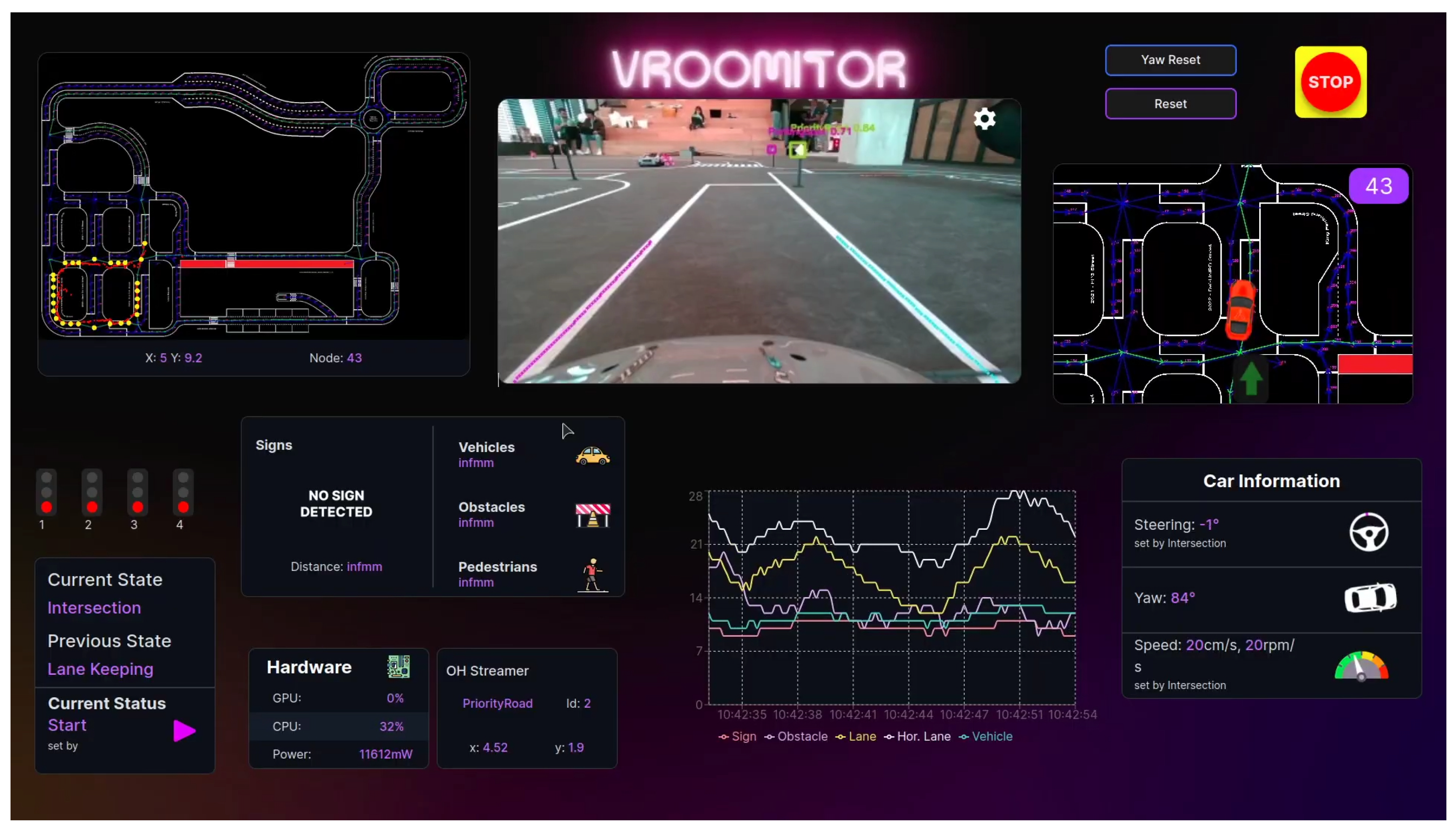
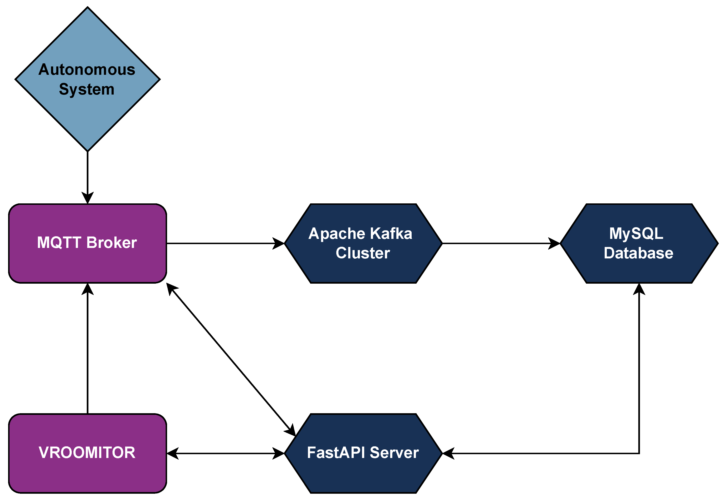
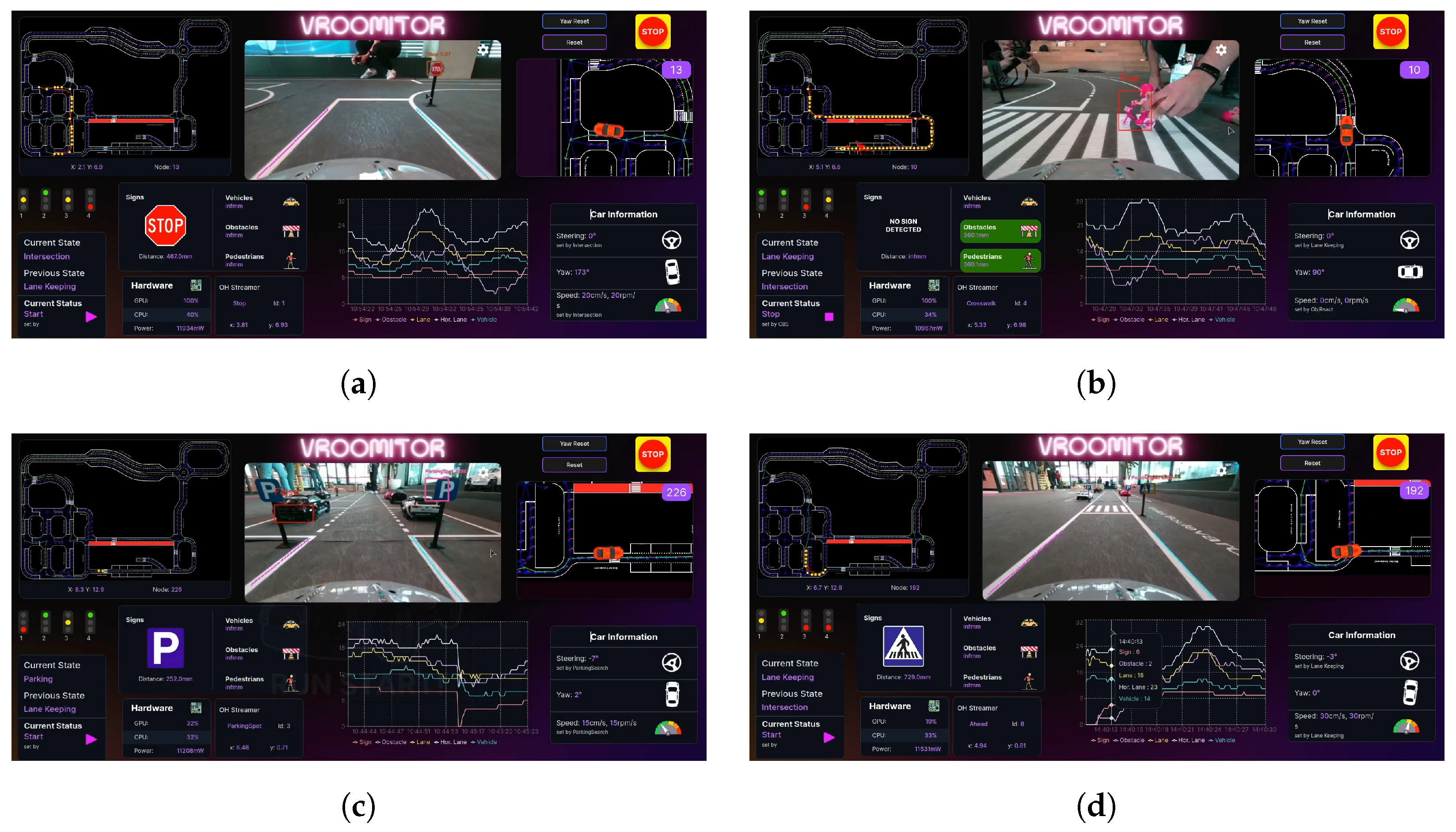
4.5. Real-Time Monitoring System

The need to track the autonomous vehicle’s hardware resources and test its software efficiency led to the development of a web application for the real-time visualization and monitoring of various data. Specifically, the application monitors hardware and power usage statistics, GPS location, car sensor readings (e.g., steering angle and yaw), frame analysis frequency for each algorithm, live camera feed, and the global vehicle state. In addition to monitoring, the application provides functionalities to signal an emergency stop, reset vehicle state variables, and control which data is being transmitted. The app is also used as the front-end for a software-in-the-loop method, allowing both the visualization of the results and control over the inputs, resulting in an optimal tool for testing. Importantly, the application is designed to be easily accessible from any device without requiring installation and supports multiple vehicles.
React was selected as the frontend framework, hosted locally in the lab, responsible for the application’s user interface, and an EMQX MQTT Broker [33] was employed, hosted on the vehicle, responsible for data exchange between the car and the application. The data sent from the vehicle to the application and vice versa is separated into multiple broker topics (streams), organized by size, importance, and relevance.
The central component of the application is the live camera feed, which supports camera switching and mode selection (depth or color). This feed is projected between the map (on the left) and minimap (on the right) as shown in Figure 23. Above the minimap, users can find the “Emergency Stop”, “Reset”, and “Yaw Reset” buttons for emergency control access. The lower half of the screen contains components that provide key information, including, traffic light status, vehicle’s state, current detections, and hardware statistics. There is also a line chart, representing the frame processing rate of each algorithm. Finally, pressing the "VROOMITOR" logo opens a settings window where users can configure options such as the broker’s IP address, the configuration file of the vehicle and enable the replay mode, which is described in the next section.

4.6. Run–Replay Function

Following each run, all data generated or utilized by the vehicle are automatically saved in a database hosted on the lab’s server. When the run–replay mode is enabled, real-time sensor data is replaced by this stored dataset, with the same timestamps preserved. This effectively simulates the vehicle’s run, enabling algorithms to be tested in a controlled, repeatable environment without relying on live sensor input. By replaying specific sessions, we can analyze and fine-tune our system under identical conditions, ensuring a more accurate review process. One of the major advantages of this feature is that it allows the vehicle to “re-run” without any physical presence on the track.
The architecture of the run–replay function is as follows:
  • Data Transmission: During each run, the vehicle transmits all relevant data through an MQTT broker to VROOMITOR.
  • Data Storage: The replay server subscribes to the corresponding MQTT broker topics and re-transmits the data via an Apache Kafka cluster, which acts as an intermediary. The data is then processed and ingested by an Apache Flink cluster, both hosted on the team’s main Ubuntu server in the lab. The processed telemetry data is organized into sessions—each representing a complete vehicle run—and stored in a MySQL database.
  • Replay Selection: When the vehicle switches to replay mode, the user selects the desired session through VROOMITOR. The FastAPI server then responds to the vehicle with the stored data from that session, ensuring accurate timestamp replication.
  • Data Utilization: Instead of using live sensor input, the vehicle processes the replayed data with preserved timestamps as though it were in real time. The entire software architecture operates normally, with all modules functioning as if the data originated from the vehicle’s sensors during a live run.
A simplified diagram of the replay function architecture is presented in Figure 24.

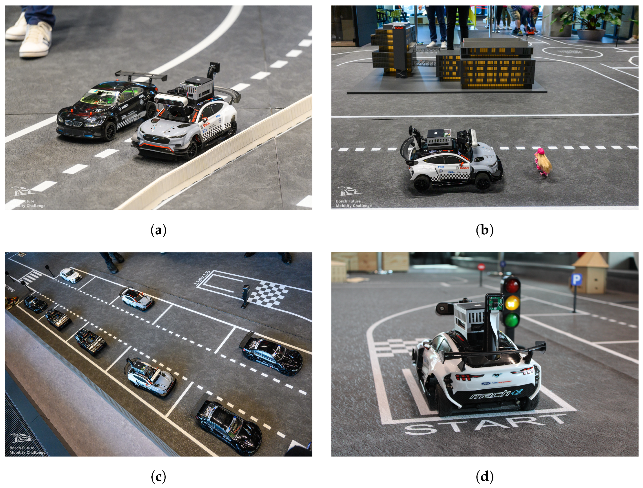
5. Outcomes and Showcase

The team participated in the BFMC-2024, developing the described solutions over a period of six months, from November 2023 to May 2024. Initially, more than 80 teams entered the competition. After the qualifications phase, only 23 teams advanced to the semi-finals, earning the opportunity to compete at the Bosch Engineering Center in Cluj-Napoca, Romania. Over the course of a rigorous 3-day testing period on the competition track (as shown in Figure 25), the team refined their vehicle’s performance, ensuring that it met the challenging demands of the event.
Reaching the finals as one of the top eight teams, the vehicle delivered an impressive and nearly flawless run. Despite two minor penalties for touching the track lines, the team demonstrated exceptional control and precision.
The statistical analysis, which is presented in Table 3, represents the only viable quantitative evaluation under true competition conditions, as these were the only officially monitored, uninterrupted runs in a dynamic and realistic testbed. Due to track-size limitations and the inability to fully replicate the stochastic behaviors of the competition environment (such as moving vehicles, pedestrians, or randomized start points), repeating these experiments externally is not currently feasible.
While some module-level failures were observed, we emphasize that such events are not uncommon even in commercial-level systems—recent real-world examples include failures from high-profile autonomous solutions such as Tesla’s Full Self-Driving (FSD) software [34,35]. It is important to note that our approach aligns with SAE Level 4–5 autonomy in its architecture, but the system was deployed in an Advanced Driver Assistance System (ADAS)-like configuration for this event. Consequently, while robustness is critical, occasional failures remain acceptable within the experimental scope.
Furthermore, our goal is not to deliver a market-ready product but rather to create a research platform for exploring the intricacies of urban autonomous navigation in a controlled environment. We explicitly acknowledge that real-world deployment entails broader safety, regulatory, and reliability requirements. Instead, our focus is on progressive scalability through modular improvements, using this testbed to inform future development in both academic and applied contexts.
At this point, it is important to note that further quantitative performance metrics, including comparative baselines, could not be provided due to several key constraints. Firstly, no openly accessible implementations or datasets are available from other teams in the competition, preventing reproducible benchmarking within the same context. Secondly, most state-of-the-art or commercial autonomous systems operate with proprietary software and advanced hardware setups, often beyond the reach of our low-cost, modular platform. Finally, while the literature does offer alternative approaches, these typically involve richer sensor modalities (e.g., LIDAR) and higher compute capabilities. In order to provide a quantitative evaluation of our approach, Table 3 is introduced, including a statistical performance validation within the real-world conditions of the competition. There, we present the distinct software modules involved in our approach, and the number of times they were used during the two official runs performed in the competition, as well as their failure rates. While all modules have low failure rates, it is evident that some problems occurred during the overtake and the intersection modules, which in a real scenario would probably lead to collision. Nevertheless, we argue that if our approach is to be used as an ADAS (Advanced driver-assistance system), these drawbacks are negligible since the human will be there to manually resolve more complex or error-prone driving conditions.
Ultimately, our vehicle secured first place, a testament to the robustness and reliability of both the software and hardware solutions developed. Some screenshots taken from VROOMITOR during the semi-finals are presented in Figure 26, while some photos of the vehicle during the runs are shown in Figure 27.

6. Conclusions

In conclusion, the development of this autonomous vehicle for the BFMC represents a significant step toward advancing the field of scaled-down autonomous driving systems. Through careful integration of heterogeneous hardware and software solutions, the team achieved a reliable, high-performing vehicle capable of handling complex driving scenarios. The system’s architecture, combined with optimized algorithms, enabled the robot to perform successfully in a competitive environment, ultimately securing first place in the competition. This result not only highlights the robustness of the current system but also underscores the potential for further innovation in autonomous driving technologies, especially at the 1:10 scale, where experimentation can be more affordable and versatile.

6.1. Solution Migration to Real Systems

While the platform developed in this work is not intended to be deployed in full-sized autonomous vehicles, it serves as a valuable research and development testbed that captures many of the challenges of urban navigation. By emphasizing a software/hardware co-design with modular architecture and minimal sensing, this 1:10 scale system enables rapid and safe evaluation of algorithms and system behaviors under realistic constraints. The design decisions, such as using the Jetson Orin NX for real-time processing and the Intel RealSense D455 for 3D environment mapping, allow the exploration of real-time performance, system integration, and decision-making in a way that can inform future adaptations. The integration of robust sensor fusion, perception, and control algorithms reflects the current trends in developing autonomous vehicles capable of navigating complex urban environments with minimal human intervention. This project, although built on a 1:10 scale, offers significant insights that can be scaled up to larger autonomous vehicles. For migrating the system to larger platforms, the following practical steps would be required:
  • Updating the sensors to higher-range or more robust alternatives suitable for larger-scale vehicles.
  • Upgrading the main processor to handle the increased computational demands.
  • Retraining the neural networks with data relevant to larger environments and sensor configurations.
  • Adapting the software stack, including controller parameters and perception thresholds, to the scale and dynamics of the new platform.
  • Ensuring functional safety. As the system transitions from a testbed to a vehicle that may carry human passengers or interact with real traffic, safety assurance becomes critical. This includes incorporating fail-safes, redundancy in critical systems, and compliance with standards.
  • Integrating cybersecurity mechanisms. Full-scale autonomous vehicles must guard against threats such as data breaches, remote attacks, and system spoofing. This involves implementing secure communication protocols, encryption layers, intrusion detection systems, and regular software validation.
  • Complying with local regulatory frameworks. Deployment of real autonomous vehicles must adhere to national and international traffic laws, certification standards, and ethical guidelines. This may require adapting behaviors (e.g., speed limits and right-of-way rules) and ensuring legal traceability and accountability for system decisions.

6.2. Limitations

As is obvious, the testing environment is limited to a miniaturized track, simulating urban driving conditions. While this setup enables thorough testing of algorithms in a controlled environment, it falls short of capturing the full unpredictability of real-world scenarios. Factors such as weather changes, sensor noise, unexpected road conditions, and unpredictable behavior from other vehicles or pedestrians are not fully represented. Additionally, the testing conditions lack diversity, as the algorithms have not been extensively tested with a wide range of pedestrian and vehicle examples, such as SUVs, buses, pedestrians using canes, or parents with baby strollers. Furthermore, while the 1:10 scale vehicle model offers significant advantages in prototyping and experimentation, there are inherent limitations in scaling the findings to full-size autonomous vehicles. Certain behaviors, such as sensor precision, vehicle dynamics, and latency constraints, may not fully translate to larger models. Additionally, this research focuses on vehicle autonomy without any external human intervention during operation. However, the system’s reliance on specific communication protocols, such as MQTT for data transmission and TCP for server connections, introduces potential limitations in environments where these protocols may experience interference or performance degradation. The research also assumes a static network infrastructure with reliable communication with external servers for localization and traffic light management, which may not reflect real-world variability. Lastly, while the algorithms are designed to handle a variety of tasks, the system prioritizes certain actions, such as pedestrian safety, which may lead to trade-offs in speed and efficiency.

6.3. Future Work

For the next phase of the research, the team is set to focus on optimizing the existing algorithms, particularly in terms of speed and efficiency, while maintaining the core architecture that has already proven reliable. A key goal is to introduce new advanced features that will significantly enhance the vehicle’s autonomous capabilities. These features include tunnel navigation, intersection and roundabout handling with moving vehicles, overtaking vehicles coming from the opposite direction, navigating in foggy environments, performing various parking maneuvers, and achieving self-localization using purely IMU- and Visual-based methods. To effectively implement these features, additional hardware will be integrated to increase system robustness and ensure the highest levels of safety. Furthermore, power efficiency remains a top priority, with plans to redesign the power management system and possibly introduce a second battery. This approach will ensure that the vehicle remains scalable and capable of handling future challenges in the autonomous driving landscape. With this extensive roadmap, the team is preparing for a challenging but promising course.

Author Contributions

Conceptualization, T.P., E.T. and A.L.S.; methodology, T.P., E.T. and A.L.S.; software, T.P., A.N., A.P., D.C. and I.G.; validation, T.P., A.N. and E.T.; investigation, T.P. and E.T.; data curation, T.P., A.N., A.P. and D.C.; writing—original draft preparation, T.P., A.N., A.P., D.C. and I.G.; writing—review and editing, T.P., E.T. and A.L.S.; visualization, I.G.; supervision, E.T. and A.L.S.; funding acquisition, T.P., A.N., A.P. and D.C. All authors have read and agreed to the published version of the manuscript.

Funding

This research was mainly funded by the Research Committee of Aristotle University of Thessaloniki, Greece. Further funding in the form of donations was received from the companies Altair, DEI, KEBE, Kenotom, BOSCH Greece, Laboratory of NeuroMechanics-AUTH, and Cyclopt.

Data Availability Statement

Dataset available on request from the authors.

Acknowledgments

We would like to acknowledge the technical support of the ISSEL labgroup, Aristotle University of Thessaloniki, Greece, as well as the provision of space to host our team, and perform our experiments by the School of Electrical and Computer Engineering, Aristotle University of Thessaloniki, Greece.

Conflicts of Interest

The authors declare no conflicts of interest.

Abbreviations

The following abbreviations are used in this manuscript:
3D 3-Dimensional
ADASAdvanced Driver Assistance System
AIArtificial Intelligence
AVAutonomous Vehicle
BFMCBosch Future Mobility Challenge
DRLDeep Reinforcement Learning
ESCElectronic Speed Controller
FFFFused Filament Fabrication
FFCFlexible Flat Cable
FPSFrames per second
FSDFull Self-Driving
FSMFinite State Machine
GPSGlobal Positioning System
GUIGraphical User Interface
IMUInertial Measurement Unit
LiPoLithium-Polymer
PIDProportional–Integral–Derivative
PIProportional–Integral
PWMPulse Width Modulation
RCRemote-controlled
ROSRobot Operating System
SAESociety of Automotive Engineers
SLAMSimultaneous Localization and Mapping
TCPTransmission Control Protocol
ToFTime-of-Flight
UDPUser Datagram Protocol
YOLOYou Only Look Once

References

  1. Singh, S. Critical Reasons for Crashes Investigated in the National Motor Vehicle Crash Causation Survey. In Proceedings of the National Motor Vehicle Crash Causation Survey (NMVCCS) U.S. Department of Transportation, 1 February 2015. Available online: https://crashstats.nhtsa.dot.gov/Api/Public/ViewPublication/812115 (accessed on 10 June 2025).
  2. Kalra, N.; Paddock, S.M. Driving to safety: How many miles of driving would it take to demonstrate autonomous vehicle reliability? Transp. Res. Part Policy Pract. 2016, 94, 182–193. [Google Scholar] [CrossRef]
  3. McKinsey & Company. Ten Ways Autonomous Driving Could Redefine the Automotive World. 2015. Available online: https://www.mckinsey.com/industries/automotive-and-assembly/our-insights/ten-ways-autonomous-driving-could-redefine-the-automotive-world (accessed on 9 October 2024).
  4. Williams, M. PROMETHEUS-The European research programme for optimising the road transport system in Europe. In Proceedings of the IEE Colloquium on Driver Information, London, UK, 1 December 1988; pp. 1–9. [Google Scholar]
  5. DARPA. DARPA News & Events. 2014. Available online: https://www.darpa.mil/news-events/2014-03-13 (accessed on 2 September 2024).
  6. Fulton, J.; Pransky, J. DARPA Grand Challenge—A pioneering event for autonomous robotic ground vehicles. Ind. Robot 2004, 31, 414–422. [Google Scholar] [CrossRef]
  7. Buehler, M.; Iagnemma, K.; Singh, S. The DARPA Urban Challenge: Autonomous Vehicles in City Traffic; Springer Tracts in Advanced Robotics; Springer: Berlin/Heidelberg, Germany, 2009; Volume 56. [Google Scholar]
  8. SAE. Taxonomy and Definitions for Terms Related to Driving Automation Systems for On-Road Motor Vehicles; Techology Report J3016; SAE International: Warrendale, PA, USA, 2021. [Google Scholar]
  9. Yurtsever, E.; Lambert, J.; Carballo, A.; Takeda, K. A Survey of Autonomous Driving: Common Practices and Emerging Technologies. IEEE Access 2020, 8, 58443–58469. [Google Scholar] [CrossRef]
  10. Wayve. Wayve AV2.0 Technology. 2024. Available online: https://wayve.ai/technology/#AV2.0 (accessed on 11 October 2024).
  11. Bojarski, M.; Testa, D.D.; Dworakowski, D.; Firner, B.; Flepp, B.; Goyal, P.; Jackel, L.D.; Monfort, M.; Muller, U.; Zhang, J.; et al. End to End Learning for Self-Driving Cars. arXiv 2016, arXiv:1604.07316. [Google Scholar] [CrossRef]
  12. Xu, H.; Gao, Y.; Yu, F.; Darrell, T. End-to-end Learning of Driving Models from Large-scale Video Datasets. arXiv 2017, arXiv:1612.01079. [Google Scholar] [CrossRef]
  13. Bojarski, M.; Yeres, P.; Choromanska, A.; Choromanski, K.; Firner, B.; Jackel, L.; Muller, U. Explaining How a Deep Neural Network Trained with End-to-End Learning Steers a Car. arXiv 2017, arXiv:1704.07911. [Google Scholar] [CrossRef]
  14. Koutník, J.; Cuccu, G.; Schmidhuber, J.; Gomez, F.J. Evolving large-scale neural networks for vision-based TORCS. In Proceedings of the International Conference on Foundations of Digital Games, Crete, Greece, 14–17 May 2013. [Google Scholar]
  15. Sallab, A.E.; Abdou, M.; Perot, E.; Yogamani, S. Deep Reinforcement Learning framework for Autonomous Driving. Electron. Imaging 2017, 29, 70–76. [Google Scholar] [CrossRef]
  16. Kendall, A.; Hawke, J.; Janz, D.; Mazur, P.; Reda, D.; Allen, J.M.; Lam, V.D.; Bewley, A.; Shah, A. Learning to Drive in a Day. arXiv 2018, arXiv:1807.00412. [Google Scholar] [CrossRef]
  17. Lu, Y.; Fu, J.; Tucker, G.; Pan, X.; Bronstein, E.; Roelofs, R.; Sapp, B.; White, B.; Faust, A.; Whiteson, S.; et al. Imitation Is Not Enough: Robustifying Imitation with Reinforcement Learning for Challenging Driving Scenarios. arXiv 2023, arXiv:2212.11419. [Google Scholar] [CrossRef]
  18. Li, D.; Auerbach, P.; Okhrin, O. Towards Autonomous Driving with Small-Scale Cars: A Survey of Recent Development. arXiv 2024, arXiv:2404.06229. [Google Scholar] [CrossRef]
  19. Balaji, B.; Mallya, S.; Genc, S.; Gupta, S.; Dirac, L.; Khare, V.; Roy, G.; Sun, T.; Tao, Y.; Townsend, B.; et al. DeepRacer: Autonomous Racing Platform for Experimentation with Sim2Real Reinforcement Learning. In Proceedings of the 2020 IEEE International Conference on Robotics and Automation (ICRA), Paris, France, 31 May–31 August 2020; pp. 2746–2754. [Google Scholar] [CrossRef]
  20. Paull, L.; Tani, J.; Ahn, H.; Alonso-Mora, J.; Carlone, L.; Cap, M.; Chen, Y.F.; Choi, C.; Dusek, J.; Fang, Y.; et al. Duckietown: An open, inexpensive and flexible platform for autonomy education and research. In Proceedings of the 2017 IEEE International Conference on Robotics and Automation (ICRA), Singapore, 29 May–3 June 2017; pp. 1497–1504. [Google Scholar] [CrossRef]
  21. Berkeley Autonomous Race Car (BARC). BARC: Berkeley Autonomous Race Car. Available online: https://goldeneye.studentorg.berkeley.edu/barc.html (accessed on 28 August 2024).
  22. O’Kelly, M.; Sukhil, V.; Abbas, H.; Harkins, J.; Kao, C.; Pant, Y.V.; Mangharam, R.; Agarwal, D.; Behl, M.; Burgio, P.; et al. F1/10: An Open-Source Autonomous Cyber-Physical Platform. arXiv 2019, arXiv:1901.08567. [Google Scholar] [CrossRef]
  23. Goldfain, B.; Drews, P.; You, C.; Barulic, M.; Velev, O.; Tsiotras, P.; Rehg, J.M. AutoRally: An Open Platform for Aggressive Autonomous Driving. IEEE Control Syst. Mag. 2019, 39, 26–55. [Google Scholar] [CrossRef]
  24. F1TENTH Autonomous Racing. F1TENTH Racing. Available online: https://f1tenth.org/race.html (accessed on 28 August 2024).
  25. Bosch Engineering Center, C. Bosch Future Mobility Challenge. Available online: https://boschfuturemobility.com/ (accessed on 10 September 2024).
  26. Stanford-Clark, A.; Nipper, A. MQTT Version 3.1.1. OASIS Standard. 2014. Available online: http://docs.oasis-open.org/mqtt/mqtt/v3.1.1/os/mqtt-v3.1.1-os.html (accessed on 1 February 2025).
  27. Systèmes, D. SolidWorks. Version 2023. Dassault Systèmes. 2023. Available online: https://www.solidworks.com/ (accessed on 20 February 2025).
  28. Boyer, R.S.; Moore, J.S. A Fast String Searching Algorithm. Commun. ACM 1977, 20, 762–772. [Google Scholar] [CrossRef]
  29. Wang, C.Y.; Liao, H.Y.M. YOLOv9: Learning What You Want to Learn Using Programmable Gradient Information. arXiv 2024, arXiv:2402.13616. [Google Scholar]
  30. Bao, W.; Ma, Z.; Liang, D.; Yang, X.; Niu, T. Pose ResNet: 3D Human Pose Estimation Based on Self-Supervision. Sensors 2023, 23, 3057. [Google Scholar] [CrossRef] [PubMed]
  31. Takahashi, A.; Hongo, T.; Ninomiya, Y.; Sugimoto, G. Local Path Planning And Motion Control For Agv In Positioning. In Proceedings of the IEEE/RSJ International Workshop on Intelligent Robots and Systems. (IROS ’89) ’The Autonomous Mobile Robots and Its Applications, Tsukuba, Japan, 4–6 September 1989; pp. 392–397. [Google Scholar] [CrossRef]
  32. Foead, D.; Ghifari, A.; Kusuma, M.B.; Hanafiah, N.; Gunawan, E. A Systematic Literature Review of A* Pathfinding. Procedia Comput. Sci. 2021, 179, 507–514. [Google Scholar] [CrossRef]
  33. EMQ Technologies Co., Ltd. EMQX: Cloud-Native Distributed MQTT Message Broker. 2024. Available online: https://www.emqx.io (accessed on 24 May 2025).
  34. Guardian, T. Tesla Autopilot Was Involved in 13 Fatal Crashes, US Agency Finds. 2024. Available online: https://www.theguardian.com/technology/2024/apr/26/tesla-autopilot-fatal-crash (accessed on 24 May 2025).
  35. Lambert, F. Tesla Full Self-Driving Veers Off Road, FLIPS car in Scary Crash Driver Couldn’t Prevent. 2025. Available online: https://electrek.co/2025/05/23/tesla-full-self-driving-veers-off-road-flips-car-scary-crash-driver-couldnt-prevent/ (accessed on 24 May 2025).
Figure 1. The typical BFMC track configuration, spanning 20 × 14 m and incorporating urban intersections, highway segments, parking spaces, and moving entities such as pedestrians and vehicles.
Machines 13 00514 g001
Figure 2. Hardware architecture of the autonomous vehicle, illustrating the integration of all onboard components and their connectivity. With purple color are the main computational units, with dark blue the auxiliary hardware components and with red the main power source.
Machines 13 00514 g002
Figure 3. Upgraded team vehicle compared to initial kit. (a) Top–down view highlighting the new sensor configuration; (b) perspective view of the upgraded vehicle.
Machines 13 00514 g003
Figure 4. Selected 3D-printable components designed for the vehicle using SolidWorks. All parts are optimized for FFF 3D printing.
Machines 13 00514 g004
Figure 5. Layered software architecture of the autonomous vehicle, comprising four key modules: Input, Perception, Control, and Output. The diagram illustrates the data flow from sensor acquisition and environmental understanding, through decision-making and action planning, to the final execution of motion commands.
Machines 13 00514 g005
Figure 6. Asynchronous execution structure of the software architecture, illustrating the use of multiprocessing and multithreading within each process.
Machines 13 00514 g006
Figure 7. Finite State Machine (FSM) governing the vehicle’s high-level behavior selection. The default state is Lane Keeping, from which the system transitions to task-specific states. After completing each maneuver, the system reverts to the Lane-Keeping state to maintain continuous, stable navigation.
Machines 13 00514 g007
Figure 8. Visual representation of the key metrics used for detecting points along a lane. (a) Ascent point value; (b) candidate sample; (c) plateau value; (d) pixels to plateau value.
Machines 13 00514 g008
Figure 9. Overview of the lane detection process steps. (a) Points detection; (b) DBSCAN clustering; (c) polynomials fitting.
Machines 13 00514 g009
Figure 10. Flowchart detailing the Lane Detection module, including image preprocessing, point extraction, clustering, and polynomial fitting for lane estimation.
Machines 13 00514 g010
Figure 11. Illustration of the adjustable gain problem. Without slope-based gain adjustment, off-angle entries into straight roads are misinterpreted as sharp turns, leading to instability. (a) Off-angle in a straight road; (b) sharp turn.
Machines 13 00514 g011
Figure 12. Visualization of detected points used to identify a crosswalk pattern from the lane detection process.
Machines 13 00514 g012
Figure 13. Step-by-step visualization of the obstacle detection pipeline. The color frame is added only as a reference. (a) Color frame; (b) depth frame with slices; (c) peaks extraction; (d) DBSCAN clustering; (e) final output.
Machines 13 00514 g013
Figure 14. Examples of trajectory generation between entry and exit points identified on the map graph using Cubic Hermite Splines and Bezier curves for navigating intersections and roundabouts. (a) Cubic Hermite Spline example; (b) Bezier curve example.
Machines 13 00514 g014
Figure 15. Flowchart outlining the procedures for navigating intersections and roundabouts, including turn-type identification, trajectory planning, and behavior execution.
Machines 13 00514 g015
Figure 16. Detection of parked vehicles and parking spot boundaries using object and corner detection relative to odometry-based positioning. This image is the raw output of the main car’s camera and has a resolution of 848 × 480 pixels.
Machines 13 00514 g016
Figure 17. Generated parking trajectory using a Quintic Polynomial Planner. The path ensures smooth maneuvering into the detected free spot.
Machines 13 00514 g017
Figure 18. Flowchart of the Parking module, outlining the sequential decision-making and control steps used to identify a free parking spot, compute a trajectory, and execute the maneuver.
Machines 13 00514 g018
Figure 19. Step-by-step visualization of a left lane change maneuver. (a) An obstacle appears in the vehicle’s course; (b) dotted line approached; (c) approaching left lane’s center; (d) correcting the course inside lane.
Machines 13 00514 g019
Figure 20. Finite State Machine (FSM) representing the overtake procedure. The process monitors obstacles ahead and, when conditions allow, transitions through lane change, overtaking, and reintegration phases.
Machines 13 00514 g020
Figure 21. Illustrative examples of ’must-nodes’ sets on the competition map, corresponding to the required navigation tasks. Each set defines key locations that the vehicle must traverse to complete objectives such as the roundabout or speedrun segments. (a) Roundabout; (b) speedrun.
Machines 13 00514 g021
Figure 22. Visualization of the path planning process. (a) Grouped must-node sets corresponding to required task areas; (b) final computed path formed by sequentially connecting sub-paths between selected must-nodes.
Machines 13 00514 g022
Figure 23. Web-based real-time monitoring system developed for autonomous vehicle testing. The interface displays data from the vehicle and supports remote control features and software-in-the-loop testing, with communication handled via an MQTT broker architecture.
Machines 13 00514 g023
Figure 24. Architecture of the run–replay functionality, illustrating the flow from real-time vehicle data transmission to session-based storage and replay.
Machines 13 00514 g024
Figure 25. Map of the BFMC-2024 competition track used during the semi-finals and finals at the Bosch Engineering Center.
Machines 13 00514 g025
Figure 26. Screenshots from VROOMITOR during the BFMC-2024 semi-finals, showcasing some of the autonomous behaviors. (a) Approaching STOP at intersection; (b) stopping for pedestrian on crosswalk; (c) entering parking space; (d) approaching crosswalk.
Machines 13 00514 g026
Figure 27. Photos from the BFMC-2024 competition. (a) Overtaking; (b) Pedestrian Stop; (c) Parking; (d) Starting Position.
Machines 13 00514 g027
Table 1. Tasks and scoring.
TaskPointsMandatoryDescription
Parking8YesIdentifying suitable parking spots and executing parking maneuvers.
Ramp5YesDriving on an inclined surface.
Roundabout7YesNavigating the roundabout counter-clockwise.
Traffic lights6YesRecognizing and reacting to traffic lights.
Missing lanes6NoNavigating safely in areas with only partial road markings.
Bus lane5NoNot entering the adjacent bus lane on the left.
Highway5NoMaintaining position in the right lane, except when executing
an overtaking maneuver.
Speed curve7NoIncreasing speed on a curved road while slowing down or stopping
at crosswalks as required.
Random start point15NoStarting at a random point inside the competition map.
Table 2. Penalties.
Table 2. Penalties.
PenaltyPointsDescription
Collision−2Colliding with another vehicle, pedestrian, or structure.
Non-compliance with traffic rules−1.5Ignoring traffic lights or signs.
Maneuver fail−1Incorrect or incomplete parking, hit on overtaking comeback,
initiating parking where it shouldn’t be.
Table 3. Module performance analysis over 26 min of semi-final and final runs.
ModuleCallsFailuresFailure Rate (%)Impact
Intersection2015High
Roundabout600.0High
Overtake (static vehicle)4125High
Overtake (dynamic vehicle)400.0High
Pedestrian Reaction1000.0High
Traffic Lights Reaction900.0High
Sign Reaction2000.0Medium
Path Planning3000.0High
Lane Detection-Keeping10022High
Crosswalk Detection500.0Medium
Parking300.0High
Speed Adaptation40110.0Small
3D-Object Detection7011.4Medium
Disclaimer/Publisher’s Note: The statements, opinions and data contained in all publications are solely those of the individual author(s) and contributor(s) and not of MDPI and/or the editor(s). MDPI and/or the editor(s) disclaim responsibility for any injury to people or property resulting from any ideas, methods, instructions or products referred to in the content.

