SiMBA-Augmented Physics-Informed Neural Networks for Industrial Remaining Useful Life Prediction

Abstract

Remaining useful life (RUL) prediction of industrial equipment is critical for achieving safe operations and optimizing predictive maintenance. To tackle the limitations of poor interpretability, inaccurate predictions, and high computational cost in complex system degradation modeling, this paper proposes SiMBA-PINN, a novel fusion framework that synergizes Physics-Informed Neural Network (PINN) with an enhanced state-space model (SiMBA). The framework achieves dynamic fusion of data-driven features and physical laws through a two-branch synergistic mechanism: the temporal modeling branch combines selective state-space SiMBA with Einstein Fast Fourier Transform (EinFFT)-based spectral mixing to efficiently capture cross-sensor temporal dependencies and degradation trends, while the physics-constraint branch embeds automatically differentiable partial differential equation residuals derived from domain-specific degradation mechanisms, enforcing physical consistency through deep hidden physics modeling. Here, the EinFFT-based spectral mixing leverages frequency-domain interactions to effectively blend the spectral components of multivariate time-series data, thereby enhancing the modeling of cross-sensor dependencies. Meanwhile, deep hidden physics modeling integrates physics-informed partial differential equation (PDE) residuals through differentiable operators, aligning the learned representations with domain-specific dynamics via a constraint-driven loss design. Experimental results from the C-MAPSS dataset confirm that the proposed model significantly outperforms PINN-, Mamba- and attention mechanism-based models, achieving State-of-the-Art RMSE on the most challenging FD004 subset. This physics-aware framework achieves deployable and interpretable RUL prediction by balancing accuracy with linear-time complexity.

1. Introduction

Progressive degradation of industrial equipment may precipitate catastrophic safety incidents and substantial economic losses. The degradation process of industrial equipment presents non-linear, multi-modal, and high noise characteristics. The complexity of equipment and its operating environment is also becoming more complex and variable. The primary job in machinery health monitoring of industrial equipment is predicting remaining usable life (RUL), which has a direct bearing on production safety, operation and maintenance safety, and financial gains.

Currently, RUL prediction methods fall primarily into physics-based models [1], data-driven algorithms [2,3,4,5], and hybrid methods [6,7]. Physics-based models require precise modeling of material aging and environmental coupling processes, yet their application is often limited by the high computational costs and poor generalizability caused by multi-factor interactions in complex systems. For instance, aging phenomena in nuclear power plant equipment involve coupled thermo-chemical processes that cannot be adequately described by single-equation models. Deep learning has emerged as a pivotal technology for data- driven RUL prediction due to its superior feature extraction capabilities. To address industrial challenges such as data scarcity and heterogeneity, researchers have developed multi-source information fusion frameworks. Notably, the Deep Spatiotemporal Network (DSTN) with interactive attention mechanisms dynamically integrates vibration signals with time-varying operational data. By extracting spatiotemporal features and employing adaptive weight mechanisms, this approach achieves a 30% reduction in prediction error on refinery rotating machinery datasets [8]. Similarly, cascaded models where Principal Component Analysis (PCA)-reduced features are processed by Convolutional Neural Networks (CNN) and Bidirectional Long Short-Term Memory (Bi-LSTM) layers have demonstrated cross-dataset generalization capabilities on NASA and CALCE battery datasets [9]. However, neural network-based methods for RUL prediction still face issues such as poor interpretability and high computational resource consumption. Therefore, enhancing the interpretability of neural network models, particularly through the integration of physical models or the use of visualization techniques to understand the relationship between features and prediction outcomes, is a key focus of current research.

Emerging hybrid RUL prediction architectures, including physics-constrained neural networks, combine data-driven machine learning approaches with physical system equation constraints, demonstrating practical implementation success. Physics-Informed Neural Network (PINN) synergizes physical equations with neural networks to achieve co-optimization of data-driven learning and physical principles, offering novel solutions for enhancing the interpretability and robustness of RUL prediction. Raissi et al. [10] proposed a deep learning framework that embeds partial differential equation (PDE) physical constraints into neural networks, directly coupling PDE residuals through a loss function to achieve forward solving of nonlinear PDEs and inverse parameter inversion, thereby reducing the need for large-scale data. Cofre-Martel et al. [11] combined deep learning with PDE models to construct device degradation dynamics equations using latent variables, achieving residual life prediction and interpretable analysis of degradation mechanisms, and providing a solution that integrates data and physical laws for complex system health management. Sun et al. [12] developed a hybrid framework integrating adaptive evolutionary algorithms with PINN, which dynamically maps lithium-ion battery physics to capacity degradation processes. This approach concurrently optimized initial model parameters and updated time-varying mapping relationships during long-term operation, significantly improving health status and RUL prediction reliability. Wang et al. [13] designed a universal PINN architecture by embedding empirical degradation models and state-space equations into neural networks. Their method extracted statistical features from short-term charging data, addressing generalization challenges across battery chemistries and charging protocols, with robustness validated through few-shot learning and cross-chemical migration experiments. For imbalanced data scenarios, Qin et al. [14] employed an inverse PINN to identify bearing dynamic model parameters, generating high-fidelity fault vibration data. Coupled with digital twin technology, this enhanced cross-operational condition diagnostic precision, establishing a high-quality data foundation for RUL prediction in complex mechanical systems. However, current PINN-based RUL prediction methods still face issues such as low prediction accuracy and limited generalization ability. Designing more flexible fusion strategies and properly balancing physical information with data-driven models to enhance prediction accuracy and robustness is a key issue in current research.

Recent advances in State Space Models (SSMs) have provided breakthroughs for long-sequence modeling. Ran et al. [15] developed an innovative deep latent-variable SSM architecture that integrates Variational Autoencoders (VAE) with Gated Recurrent Units (GRU). Their framework employs differential pre-transformation to extract degradation rate features, followed by the construction of state transition equations specifically modeling the evolution of degradation rates. This framework achieved high-precision RUL prediction on both the PRONOSTIA dataset and wind turbine bearing data, with its probabilistic modeling approach significantly enhancing generalization under complex operating conditions. Representative SSMs, such as Mamba, employ selective state propagation mechanisms to achieve global context awareness with linear complexity. Qiao et al. [16] introduced the first Mamba-based multimodal large language model framework, replacing traditional Transformer backbones with Mamba language models and incorporating Visual Selective Scanning (VSS) modules to strengthen multimodal representation learning. Experiments demonstrated comparable or superior performance to existing models in image classification and text generation tasks, validating Mamba’s potential for multimodal applications. Building on this, Dao and Gu [17] unified SSMs with attention mechanisms through Structured State-space Duality (SSD) theory, proposing the Mamba-2 architecture. While maintaining performance parity with Transformers, this model achieved 2–8 × faster training speeds and revealed intrinsic connections between SSMs and attention mechanisms, offering new perspectives for algorithmic optimization. Zhu [7] proposed MAMBA-PINN, a novel hybrid framework for RUL prediction, which was rigorously validated on the C-MAPSS dataset.

However, Mamba exhibits stability limitations due to: (1) inefficient parameter utilization caused by high-dimensional feature representations, and (2) insufficient cross-channel information interaction. These constraints collectively degrade its performance in complex industrial scenarios. Recently, the SiMBA architecture, introduced by Patro and Agneeswaran [18], significantly enhances model stability and computational efficiency through the Einstein Fast Fourier Transform (EinFFT)-based frequency-domain channel mixing technique, enabling efficient modeling of multivariate time series. Inspired by references [6,18], this paper integrates SiMBA with PINNs to construct a novel SiMBA-PINN framework for RUL prediction. The key innovations include:

(1)

Precise degradation feature extraction: Leveraging SiMBA’s frequency-domain channel mixing and selective state-space modeling to capture temporal degradation patterns from multi-source sensor data.

(2)

Physics-guided representation learning: Embedding physical equations to constrain network learning, ensuring implicit representations align with real-world degradation laws, thereby improving generalization in data-scarce scenarios.

(3)

Dynamic fusion mechanism: Coordinating data-driven and physics-driven information flow to prevent feature conflicts. The study provides theoretical foundations for intelligent maintenance of complex industrial systems, with significant engineering applicability and academic value.

(4)

The C-MAPSS dataset tests reveal the SiMBA-PINN model’s excellent performance.

The remainder of this paper is structured as follows: Section 2 details the SiMBA-PINN framework, including its architecture, the integration of physics-informed constraints, dataset, evaluation indicators and the experimental setup. Section 3 presents the experimental results and analysis, and the performance evaluation of the proposed method, including comparative analysis with existing models and ablation studies. Section 4 summarizes the key contributions and suggests directions for future research.

2. Materials and Methods

2.1. SiMBA-PINN Framework

Inspired by references [6,18], this paper proposes a dual-branch collaborative RUL prediction model that achieves interpretable modeling through dual constraints of data-driven approaches and physical principles. The core contribution of this work lies in the enhancement of the Deep Hidden Physics Model (DeepHPM), wherein SiMBA is employed as a surrogate model to establish a nonlinear functional mapping from the system’s hidden state space to RUL predictions. Simultaneously, the improved DeepHPM framework is utilized to uncover latent physical constraints governing the relationship between hidden states and RUL. The complete framework of SiMBA-PINN is visualized in Figure 1.

This study primarily employs a SiMBA-augmented PINN framework to predict RUL from industrial equipment sensor data. The framework incorporating a deep hidden physics model to learn latent partial differential equations (PDEs). The universal approximation capability of DeepHPM eliminates the requirement for extensive domain expertise while maintaining precise characterization of physical principles.

The RUL dynamics, as determined by the physical degradation mechanisms, are described by the following PDE:

$${\displaystyle u_t+N(u,x)=0,}$$

(1)

where $x\in {\mathbb{R}}^n,t\in [0,T]$, $N\left(u\right)$ is a nonlinear differential operator that represents the degradation dynamics of the system, and the time derivative $u_t$ is governed by the nonlinear operator N, expressed as $u_t=-N\left(u\right)$. Define the function f as:

$$f=u_t+N(u,x).$$

(2)

In physics-informed neural networks, initial conditions (IC) and boundary conditions (BC) are not strictly necessary; their presence depends on the specific nature of the problem and the training objectives. If the goal is to approximate the form of the differential equation through PINN rather than the exact solution, IC and BC may be unnecessary. On the other hand, since IC and BC are difficult to define precisely, our aim is to approximate these constraints via weighted terms in the loss function. It should be noted that this effect may be weaker than enforcing hard constraints. At this point, the PINN loss function can be written as:

$$Loss=MSE(\widehat{u},u)+\lambda MSE(\widehat{f},f),$$

(3)

where $\widehat{u}$ denotes RUL prediction result of $u(t,x)$ by the neural network and $\widehat{f}$ denotes the value of f computed from the neural network’s output.

The x-NN neural network architecture consists of a self-attention module, a layer normalization unit, and a fully connected mapping layer to form a three-level feature transformation structure [6]. In the data processing flow, the original high-dimensional perceptual data are firstly reorganized into features through the multi-head self-attention mechanism, which effectively captures the nonlinear associations among features by computing the attention weight matrix among the input sequence elements in parallel. A linear mapping is applied to the input features, yielding the Query, Key, and Value representations, and the attention distribution is obtained by scaling dot product operation, which can be formally expressed as:

$$\mathrm{Attention}(Q,K,V)=\mathrm{softmax}\left({\displaystyle \frac{Q{K}^T}{\sqrt{d_k}}}\right)V,$$

(4)

where $d_k$ is the feature dimension adjustment factor for stabilizing gradient propagation. This dynamic weight assignment mechanism based on similarity calculation significantly enhances the sensitivity to feature differences, especially when dealing with high-dimensional data with complex correlations, and enables more accurate extraction of discriminative features. The x-NN simultaneously adopts the connection method of element-by-element summation of input and output, which not only alleviates the gradient disappearance problem during deep network training, but also enhances the model characterization ability by retaining the original feature information. The subsequent normalization operation effectively accelerates the model convergence speed and improves the training stability by adjusting the mean and variance of the activation values of each neuron. Let h denote the hidden state obtained by passing the input data through the x-NN network, and y represent the true RUL value. $\widehat{y}$ is the predicted RUL value. Then, Equation (2) can be reformulated as:

$$y_t+N(y,h,y_h,y_{hh},...)=0$$

(5)

where the terms $y_h$ and $y_{hh}$ correspond to the first and second derivatives of y with respect to the hidden state h. By incorporating physical laws as soft constraints through our SiMBA-enhanced DeepHPM approach, the PINN framework enables hybrid learning of system dynamics that harmonizes observational data with physical mechanisms. The loss function Equation (3) is rewritten as:

$$Loss=MSE(\widehat{y},y)+\lambda MSE(\widehat{f},0),$$

(6)

The advantage of SiMBA lies in its EinFFT-based channel modeling module, which enables sufficient cross-channel information interaction. The architectural framework of SiMBA is demonstrated in Figure 2 [18].

The state-space model originated in the field of control theory and aims to describe the evolution laws of dynamic systems through linear differential equations. Its continuous time form can be expressed as:

$$h^{\prime }\left(t\right)=Ah\left(t\right)+Bx\left(t\right),$$

(7)

$$y\left(t\right)=Ch\left(t\right)+Dx\left(t\right),$$

(8)

where $h\left(t\right)\in {\mathbb{R}}^N$ is the hidden state vector, $x\left(t\right)\in \mathbb{R}$ is the input signal, and $y\left(t\right)\in \mathbb{R}$ is the output signal. $A\in {\mathbb{R}}^{N\times N}$ matrix controls the state transfer, $B\in {\mathbb{R}}^{N\times 1}$ and $C\in {\mathbb{R}}^{1\times N}$ are responsible for the input projection and output projection, respectively, and $D\in \mathbb{R}$ is the direct link term. The matrix D is conventionally set to zero, as the term $Dx\left(t\right)$ essentially functions as a skip connection that may lead to redundant feature learning in the state-space formulation. We employ the bilinear transformation [19] to discretize the state matrix A and B, yielding its approximated discrete-time counterpart $\overline{A}$ and $\overline{B}$:

$$h_k=\overline{A}{h}_{k-1}+\overline{B}{x}_k,$$

(9)

$$y_k=\overline{C}{h}_k,$$

(10)

where the discretization parameters $\overline{A}={(I-\Delta /2·A)}^{-1}(I+\Delta /2·A)$, $\overline{B}={(I-\Delta /2·A)}^{-1}\Delta B$, $\overline{C}=C$, and the time step $\Delta$ control the discretization accuracy. Despite the linear complexity advantage of SSM, its fixed-parameter mechanism is difficult to adapt to dynamically changing sequence patterns and suffers from gradient vanishing in long-range dependency modeling.

Mamba [20], as an improvement on SSM, addresses the limitations of traditional models through three core innovations. The first is to make the input-dependent parameters dynamic. Mamba introduces a selectivity mechanism that allows the parameters to be dynamically adjusted with the inputs:

$$h_k=\mathrm{Linear}\left(X_k\right)\in {\mathbb{R}}^N,$$

(11)

where $\mathrm{Linear}$ denotes the linear projection layer. This dynamic parameterization allows the model to adjust the state transfer behavior according to the current inputs, significantly improving the flexibility of sequence modeling. Combined with the description of the Mamba framework process in Figure 2, after passing through the linear projection layer $h_k$ is forward propagated in a residual summation:

$$s_k=\mathrm{SiLU}\left(\mathrm{Conv}\left(h_k\right)\right),$$

(12)

$$x_k=(\overline{A}{s}_{k-1}+\overline{B}{h}_k)+\mathrm{SiLU}\left(h_k\right),$$

(13)

$$y_k=\mathrm{Linear}\left(x_k\right),$$

(14)

where $\mathrm{Conv}$ denotes the convolutional layer, $s_k$ is the state representation at moment k, A is the state transfer matrix for describing the dynamics between states, and B is the input weight matrix for mapping the input features to the state space.

The second improvement is the use of parallel prefix scan for efficient training, which converts recursive computation into parallelizable matrix operations. For a sequence of length L, the computational complexity $O\left(L{N}^2\right)$ is reduced from to $O(LlogL)$. The core operation can be expressed as:

$$H=\mathrm{Segment}\mathrm{Matrix}(\overline{A},\overline{B},X),$$

(15)

$$Y=H\ast \overline{C},$$

(16)

where $\overline{C}={[C_1,C_2,\dots ,C_L]}^T$, ∗ denotes the product by position and segment matrix realizes parallel computation across time steps through chunked matrix construction.

The third improvement is the stability guarantee mechanism. The real part of the eigenvalues of the state matrix A is constrained to be negative by an exponential parameterization:

$$A=-exp\left(\widehat{A}\right)·I+\mathrm{SubDiag}\left(A_{\mathrm{tri}}\right),$$

(17)

where $\widehat{A}\in {\mathbb{R}}^N$ is the learnable parameter and SubDiag generates the lower triangular matrix. The design ensures the asymptotic stability of the system dynamics and effectively mitigates the gradient explosion problem.

For EinFFT module in SiMBA, the module processes input features $X\in {\mathbb{R}}^{H\times W\times C}$ through spectral operations. The initial spectral transformation applies 2D Fast Fourier Transform (FFT) across spatial axes, converting spatial patterns into frequency components represented as:

$$\mathcal{X}=\mathrm{FFT}\left(X\right)\in {\mathbb{C}}^{H\times W\times C},$$

(18)

where $\mathcal{X}$ contains complex-valued coefficients with magnitude and phase information. The FFT equivalently converts a local convolution operation in the spatial domain to a global product in the frequency domain, and separates the high-frequency details from the low-frequency semantics by means of the energy compression theorem, with the low-frequency components concentrated in the center region of the spectrum.

Frequency domain features are channel-mixed by a chunked diagonal parameterization strategy. The channel dimension is decomposed into $C=C_b\times C_d$, where $C_b$ is the number of chunks and $C_d$ is the subchannel dimension, and Einstein Matrix Multiplication (EMM) is performed:

$${\mathcal{Y}}^{H\times W\times C_b\times C_d}={\mathcal{X}}^{H\times W\times C_b\times C_d}⊛W^{C_b\times C_d\times C_d}.$$

(19)

It applies learnable weights $W\in {\mathbb{R}}^{C_b\times C_d\times C_d}$ independently to each sub-channel group, and ⊛ denotes the chunked matrix multiplication along the channel dimension. This reduces parameters from $O\left(C^2\right)$ to $O(C_b·C_d^2)$ while preserving cross-channel interactions through frequency domain energy compaction. The plural gating mechanism further refines the features:

$$\mathrm{Re}\left(h\right)=\sigma (\mathrm{EMM}(\mathrm{Re}\left(\mathcal{X}\right),W_r)-\mathrm{EMM}(\mathrm{Im}\left(\mathcal{X}\right),W_i)),$$

(20)

$$\mathrm{Im}\left(h\right)=\sigma (\mathrm{EMM}(\mathrm{Re}\left(\mathcal{X}\right),W_i)+\mathrm{EMM}(\mathrm{Im}\left(\mathcal{X}\right),W_r)),$$

(21)

where $h\in {\mathbb{R}}^{H\times W\times C}$ represents the activated frequency features containing both magnitude and phase adjustments, with $W_r,W_i\in {\mathbb{R}}^{C_b\times C_d\times C_d}$ being learnable real/imaginary weight matrices, and $\sigma$ is the GeLU activation function, an operation that achieves nonlinear modulation of the frequency components while preserving phase information. This operation realizes frequency-domain energy recalibration by cross-modulating the real and imaginary components to output composite features: $\mathcal{Y}=\mathrm{Re}\left(h\right)+i\mathrm{Im}\left(h\right)$.

The blended frequency domain features are mapped back to the spatial domain by an inverse FFT (IFFT):

$$Y=\mathrm{Re}\left[\mathrm{IFFT}\right(\mathcal{Y}\left)\right],$$

(22)

where $Y\in {\mathbb{R}}^{H\times W\times C}$. To guarantee the system stability, the eigenvalues of the weight matrix W are constrained to satisfy $\mathrm{Re}\left({\lambda }_i\right)<0$ to avoid the gradient explosion problem of the linear time-invariant system. This condition is realized by the negative real eigenvalues of the diagonal matrix A (state-space model parameter) at initialization, and the residual connection and dropout are used to further suppress the training oscillations and ensure that the spatial structure of the output Y is geometrically consistent with the original input.

In this framework, x-NN is responsible for mapping high-dimensional sensor data to a low-dimensional latent space through a self-attention mechanism, capturing the differences and interactions between features. DeepHPM, as the core component of the PINN, learns the underlying physical laws such as partial differential equations from the latent state and regularizes the model with physical residual terms, ensuring that the predictions align with the physical degradation process. x-NN provides a structured low-dimensional representation to DeepHPM, while DeepHPM optimizes the mapping process of x-NN through physical constraints. Together, they work synergistically to reduce the number of parameters while enhancing prediction accuracy and interpretability.

In summary, the innovation of this framework is manifested in three key aspects: (1) Cross-sensor feature synergy enhancement through frequency-domain channel mixing, addressing the inadequate fusion of multi-source heterogeneous data in conventional models. (2) Explicit embedding of differentiable physical equations to constrain network outputs with actual degradation dynamics, thereby improving generalization in small-sample scenarios. (3) Dynamic gating mechanism for adaptive weighting between data-driven and physics-informed features, preventing information conflicts caused by rigid fusion.

2.2. Dataset

The C-MAPSS dataset [21] is a NASA’s open-access dataset for aero-engine degradation simulation and is mainly used for the study of propulsion residual service life prediction algorithms. The dataset simulates the engine degradation process under different flight conditions by means of a high-fidelity aero-engine model, aiming to reproduce the performance degradation behaviour of a real engine under variable working conditions and multiple fault types.

Table 1. C-MAPSS data set statistics.

Data Set	C-MAPSS
	FD001	FD002	FD003	FD004
Training set	100	260	100	249
Testing set	100	259	100	248
Operating condition	1	6	1	6
Fault state	1	1	2	2

shows the statistical characterization of C-MAPSS dataset, which contains four sub-datasets (FD001–FD004) of increasing complexity: FD001 includes just one operating condition and one fault type: high-pressure compressor degradation, while FD004 covers six distinct operational scenarios and two failure types (high-pressure compressor degradation and the fan degradation). The processing challenges of the dataset are mainly in the operating condition bias, noise interference and complex fault coupling characteristics.

2.3. Data Processing and Feature Selection

The operating condition parameters of the training data were extracted and normalized to the range [−1, 1] through Min-Max scaling:

$$x_{\mathrm{norm}}=2·{\displaystyle \frac{x-x_{\min }}{x_{\max }-x_{\min }}}-1,$$

(23)

where $x_{min}$ and $x_{max}$ are the minimum and maximum values of this operating condition parameter in the training set and x is the original data. Applying the same normalization parameters to the test data ensures that the operating condition distributions for training and testing are consistent.

Normalized operational parameters enabled the classification of training data into various operating conditions. Both FD002 and FD004 were divided into six clusters via k-means clustering. Z-Score normalization was performed separately for sensor data within each cluster group:

$$s_{\mathrm{std}}={\displaystyle \frac{s-{\mu }_{\mathrm{group}}}{{\sigma }_{\mathrm{group}}+ϵ}},$$

(24)

where ${\mu }_{group}$ and ${\sigma }_{group}$ are the mean and standard deviation of the training data within that cluster, and $ϵ$ is a tiny constant used to prevent zero-division errors. The test data are then assigned to the nearest-neighbour groups based on the Euclidean distance of their operating condition parameters to the clustering centre, normalised with the mean and standard deviation of the corresponding group.

During the initial stages of engine operation, degradation signs are typically not evident. If the true RUL values are directly used as labels, high noise in initial-stage data may obscure degradation trend learning. Therefore, we adopt the approach from [22], utilizing a piecewise linear regression model to set the RUL labels to a threshold (constant value) at the beginning of the sequence.

Within each cycle time-series measurements of 21 sensor parameters (temperature, pressure, RPM, etc.) are recorded, as well as three adjustable operating condition, which are normalised to preserve the original model parameters. Based on the result seen in the literature [23], we select the key feature variables as shown in

Table 2. Features utilized in the proposed SiMAB-PINN model.

Variable Name	ID
Sensor signal	2, 4, 6, 7, 8, 9, 11, 12, 13, 14, 15, 17, 20, 21
Operational setting	1, 2

.

2.4. Evaluation Indicators

Two key metrics, root mean square error (RMSE) and asymmetric penalty score (Score), are utilized for effectiveness evaluation during training and testing. These two metrics reflect the accuracy of the prediction results and the risk of practical application from different perspectives, respectively, and together support a comprehensive assessment of the model’s capability.

RMSE measures the average size of the error between the predicted value and the true value, the smaller the value the more accurate the prediction. The formula is as follows:

$$RMSE=\sqrt{{\displaystyle \frac{1}{N}}\sum _{i=1}^N{\left({\widehat{y}}_i-y_i\right)}^2}.$$

(25)

Here, ${\widehat{y}}_i$ denotes the predicted RUL of the i-th sample, and $y_i$ represents its true RUL. The formula of Score is as follows:

$$Score=\left\{\begin{array}{cc}\hfill \sum _{i=1}^N\left(e^{{\displaystyle \frac{y_i-{\widehat{y}}_i}{13}}}-1\right),\hfill & \hfill \mathrm{when}{\widehat{y}}_i<y_i\hfill \\ \hfill \sum _{i=1}^N\left(e^{{\displaystyle \frac{{\widehat{y}}_i-y_i}{10}}}-1\right),\hfill & \hfill \mathrm{when}{\widehat{y}}_i\ge y_i\hfill \end{array}\right.$$

(26)

Score imposes different penalties in the direction of the prediction error, which grows exponentially when the prediction is too high, and grows slower when the prediction is too low. The penalties for the prediction error are asymmetric. In practice, high predicted values can lead to serious consequences if equipment failures are not dealt with in a timely manner, and therefore, the penalties are heavier.

2.5. Experimental Setup

The experimental platform consists of a personal computer, which was sourced from XIAOMI (Beijing, China), equipped with 12th Gen Intel(R) Core(TM) i5-12450H CPU (2.00 GHz) with 16-GB RAM, and the programming platform was python 3.10.

The processed training data is then divided into validation and training sets in 20% and 80% ratios before proceeding with model training.

Table 3. Hyperparameters of the SiMAB-PINN model.

Hyperparameters	Value	Hyperparameters	Value
Hidden state space’s dimension	4	Batch size	128
The highest order of partial derivatives	2 (FD001, FD003), 3 (FD002, FD004)	Learning rate	0.001
Fully connected layers in x-NN	2	Loss function weight ratio $\lambda$	100
Fully connected layers in DeepHPM	2	$RU{L}_{max}$	125
Fully connected layers in MLP	6	Epochs	300

details the key hyperparameter settings in this experiment. During model training we choose to use the Adan optimizer for parameter updating, which can significantly improve the model convergence speed while maintaining training stability. The hyperparameter values in Table 3 (except for batch size, learning rate, number of epochs, and $RU{L}_{max}$) were obtained through experimental tuning.

3. Results and Discussion

3.1. Results

The comprehensive experimental results across all four subsets of the C-MAPSS dataset are presented in Figure 3. These results demonstrate that the proposed model exhibits remarkable generalization capability for RUL prediction tasks. Notably, the model achieves particularly accurate predictions as equipment approaches failure, which is a critical capability for industrial intelligent fault diagnosis and prognostics.

We evaluated the proposed approach against other established PINN-, Mamba- and attention mechanism-based models, including GCU-Transformer [24], e-RULENet [25], CNN-BiLSTM-3DAttention [26], AttnPINN [6], Cau-AttnPINN [27], and Mamba-PINN [7]. The results of the comparison are presented in

Table 4. Performance comparison of various models.

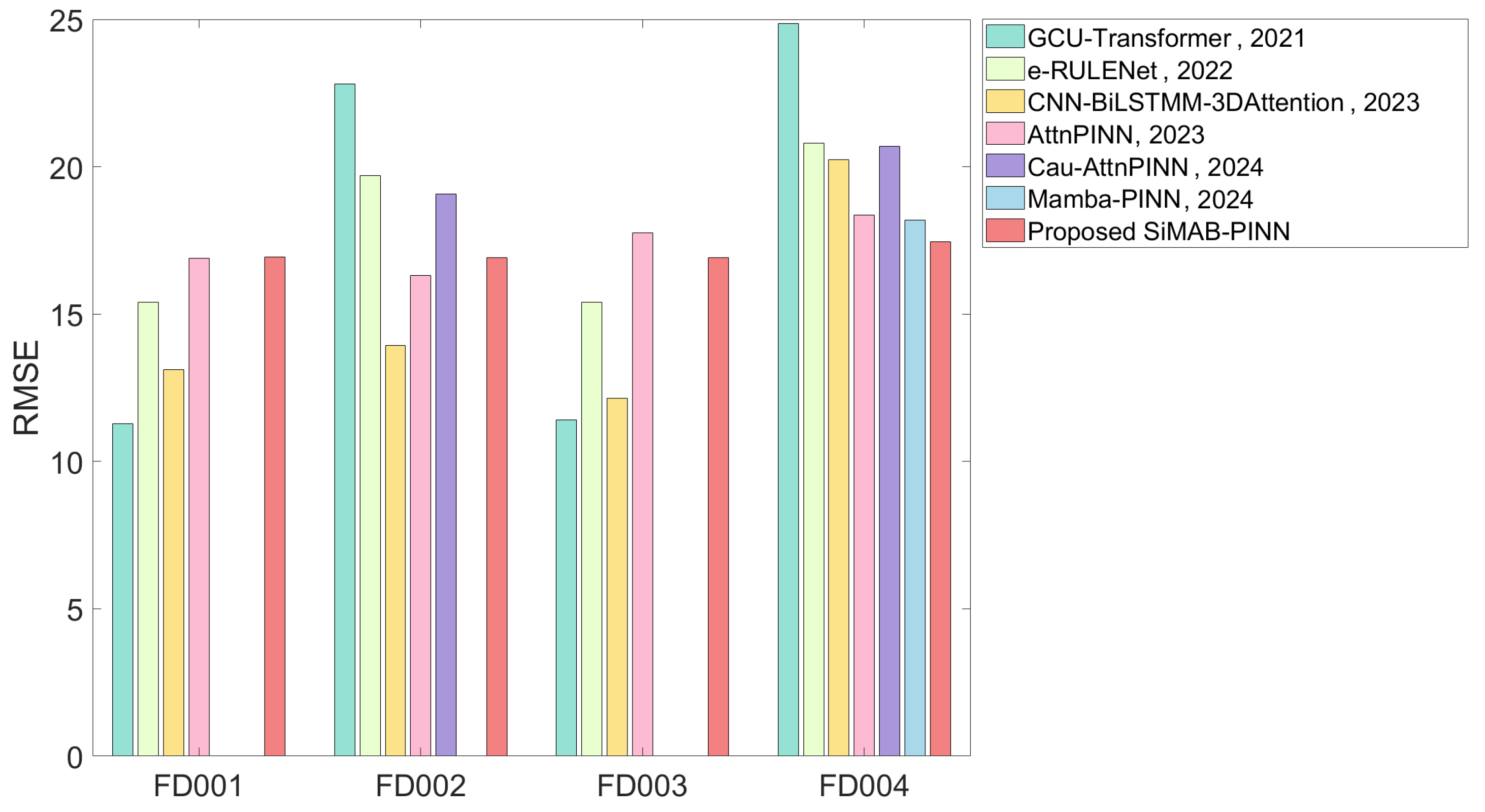
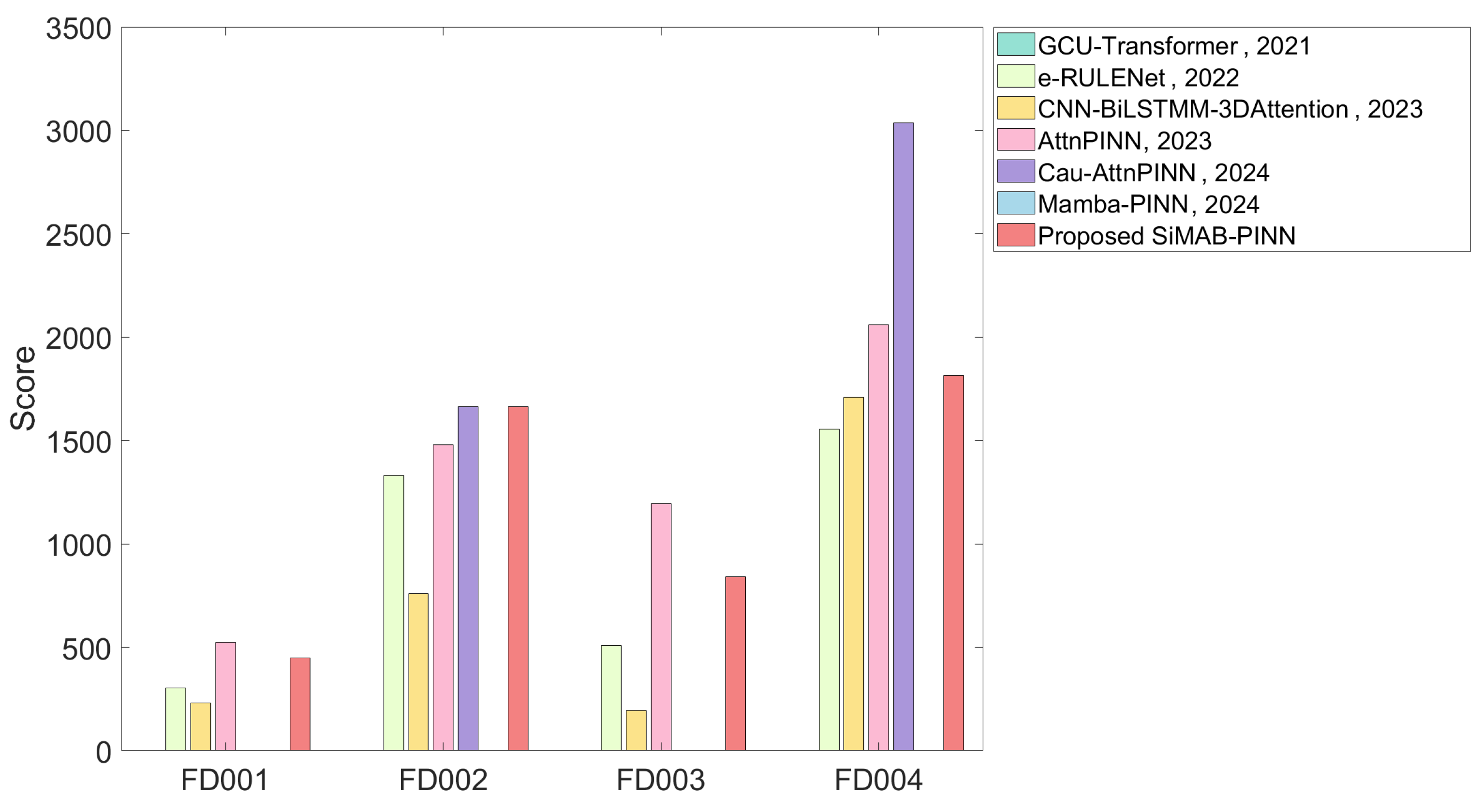
Methods	RMSE				Score
	FD001	FD002	FD003	FD004	FD001	FD002	FD003	FD004
GCU-Transformer [24], 2021	11.27	22.81	11.42	24.86	—	—	—	—
e-RULENet [25], 2022	15.40	19.70	15.50	20.80	303	1330	509	1554
CNN-BiLSTM-3DAttention [26], 2023	13.12	13.93	12.15	20.24	231	760	196	1710
AttnPINN [6], 2023	16.89	16.32	17.75	18.37	523	1479	1194	2059
Cau-AttnPINN [27], 2024	—	19.08	—	20.70	—	1665	—	3035
Mamba-PINN [7], 2024	—	—	—	18.18	—	—	—	—
Proposed SiMAB-PINN	16.94	16.91	16.92	17.45	449	1665	843	1814

N/A values are marked with “—”.

and

Table 5. Comparison of parameters and FLOPs for various models on subdataset FD004.

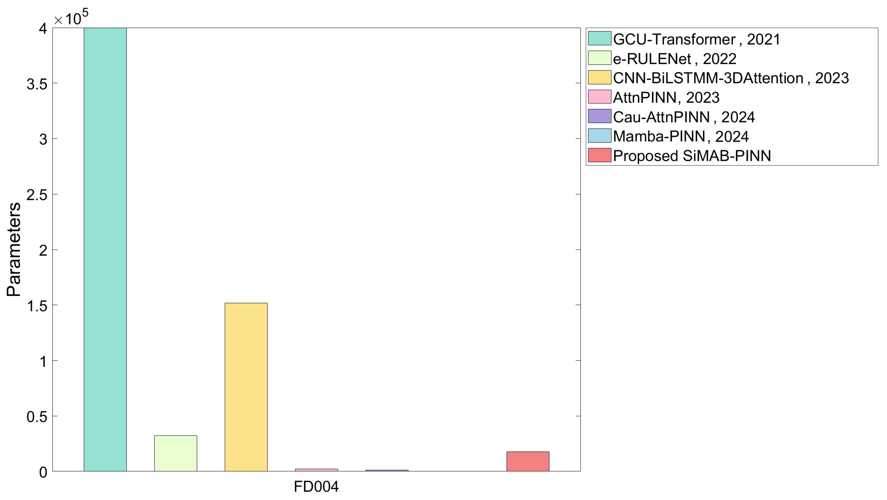
Methods	Parameters	FLOPs
GCU-Transformer [24], 2021	399.7k	393.39k
e-RULENet [25], 2022	32.3k	—
CNN-BiLSTM-3DAttention [26], 2023	151.9k	170.3k
AttnPINN [6], 2023	2260	1728
Cau-AttnPINN [27], 2024	1321	—
Mamba-PINN [7], 2024	—	—
Proposed SiMAB-PINN	17.8k	5790

N/A values are marked with “—”.

, with optimal results bolded. As evidenced by Table 4, certain models demonstrate high prediction accuracy at the cost of excessive parameters and training complexity, while simultaneously exhibiting inferior performance on the most challenging subset FD004. Conversely, other models with fewer trainable parameters achieve compromised prediction accuracy. The proposed SiMBA-PINN model effectively balances prediction precision with computational complexity. Notably, our proposed SiMBA-PINN outperforms AttnPINN across three subsets (FD001, FD003, and FD004), with marginally lower performance only on FD002. Our architecture maintains a relatively lightweight structure while achieving superior forecasting capabilities on FD004—the most complex subdataset.

To make the comparison more intuitive, we represent the RMSE, Score and parameters of the above models in histograms, respectively, as in Figure 4, Figure 5 and Figure 6. The visualization results conclusively show that our model attains an ideal equilibrium between predictive precision and computational performance, while exhibiting superior predictive performance on the most challenging FD004 dataset. Moreover, Figure 7 highlights the interpretability benefits of our prediction model.

As can be seen from Table 4 and Table 5, although the proposed model shows only slight advantages over existing data-driven RUL prediction models in terms of RMSE and Score evaluation metrics, it represents a hybrid approach that integrates physical constraints through our SiMBA-based physics-informed network framework. This integration provides notable advantages compared to recent hybrid models. The results presented in Table 5, Figure 6 and Figure 7 demonstrate that our PINN-based hybrid RUL prediction model achieves significant improvements in lightweight implementation and computational efficiency compared to purely data-driven approaches, while maintaining higher interpretability.

We will mainly utilize FD004 to analyze our proposed framework in the following. We transform the raw data into vectors in 3D space by x-NN, and map their remaining service life labels by color, and their spatial distribution characteristics are shown in Figure 7. The SiMBA-PINN-processed samples show clear inter-class separability in the potential state space, and the specific failure mode identification results are also shown in Figure 7.

The operational status of the equipment can be classified into four distinct categories: “healthy state”, “initial degradation state”, “moderate degradation state” and “severe degradation state”. The distribution of hidden states for samples in the “healthy state” is shown in dark blue in Figure 7a–c. This distribution is characterized by smaller values of x1 and x2 and a larger value of x3. The distribution of samples in the “severe degradation state” is characterized by a hidden state distribution, which is represented in the dark red region. This distribution exhibits larger values of x1 and x2, and a smaller value of x3. It is possible to determine the operational status level of the test samples intuitively from this figure. As illustrated in Figure 7d, the hidden state distribution of samples in fault mode 0 is located in the pink region, with minimal values for x1 and x2 and a substantial value for x3. The hidden state distribution of samples in fault mode 1 is situated in the light blue region, with substantial values for x1 and x2 and a negligible value for x3.

In order to visualize the model prediction performance, four engines numbered #102, #146, #194, and #213 in the FD004 subset are selected for the prediction trajectory visualization in Figure 8. Notably, the framework maintains precise monitoring of the progressive RUL deterioration in the early stage of degradation and responds quickly when a mutant type of failure occurs, and still maintains stable prediction for the samples with sensor noise interference.

3.2. Discussion

This section primarily investigates the impact of the hidden state space dimensionality and the partial derivative orders on FD004 subdataset within the proposed framework. The RMSE result for four representative cases are presented in

Table 6. Performance comparison of various hyperparameters.

Hidden State Space Dimension	Derivatives Order
	1	2	3	4
3	18.44	17.76	17.70	19.41
4	18.22	17.93	17.45	17.81
5	20.02	19.76	17.64	18.14

, comparative visualizations of the hidden state space are presented in Figure 9, while the failure mode identification results are demonstrated in Figure 10.

These ablation studies demonstrate that both latent space dimensions and the derivative orders significantly impact RUL prediction accuracy. Specifically, either an excessively large hidden dimension or insufficient derivative order compromises feature extraction capability. Notably, a 3-dimensional latent space enables intuitive visualization of sample-level RUL predictions.

As shown in Figure 7d and Figure 10, when the hidden dimension is fixed at 4, the sample hidden state distribution of failure modes becomes increasingly discrete as the derivatives order increases. When the derivatives order is fixed at 3, the sample hidden state distribution of failure modes becomes more concentrated as the hidden dimension increases.

4. Conclusions

In this study, a SiMBA-PINN framework that fuses selective state-space modeling with physical information constraints is designed to overcome the central limitations of insufficient data fusion from multiple sources, difficulty in modeling dynamic degradation, and poor generalization to small samples in the prediction of the RUL of industrial equipment. The characterization of degradation features is significantly enhanced by the synergistic modeling of frequency domain channel mixing and physical constraints. The EinFFT-based SiMBA module effectively captures the cross-channel correlation and temporal degradation trends in sensor data through frequency-domain chunked matrix operations, and reduces the RMSE to 17.45 on the C-MAPSS FD004 dataset, which is a significant improvement over the PINN-based model.

The model proposed in this paper still has some limitations: high dependence on preprocessing and standardization of sensor data; lack of external validation except for the C-MAPSS dataset; and the need for supervised labels (RUL) during training, which may not be practical in actual industrial environments. Future work will focus on two aspects: (1) Developing lightweight frequency-domain hybrid operators to reduce parameter count in the EinFFT module through low-rank decomposition, enhancing computational efficiency while maintaining performance. (2) Designing a lightweight, interpretable hybrid prediction model with high accuracy, leveraging data-driven graph structural features to balance transparency and predictive power. The aim is to deliver a novel interpretable and high-precision solution for intelligent industrial equipment maintenance. Such innovations hold significant practical value for predictive maintenance in safety-critical scenarios like nuclear power plants and satellite systems, where reliability and explainability are paramount.

References

- El-Dalahmeh, M.; Al-Greer, M.; El-Dalahmeh, M.; Bashir, I. Physics-based model informed smooth particle filter for remaining useful life prediction of lithium-ion battery. Measurement 2023, 214, 112838. [Google Scholar] [CrossRef]
- Zhao, Y.; Zhang, W.; Yan, R. Remaining Useful Life Prediction of Aero-Engine Based on Data-Driven Approach Using LSTM Network. IEEE Access 2022, 10, 25359–25370. [Google Scholar]
- Liang, P.; Li, Y.; Wang, B.; Yuan, X.; Zhang, L. Remaining useful life prediction via a deep adaptive transformer framework enhanced by graph attention network. Int. J. Fatigue 2023, 174, 107722. [Google Scholar] [CrossRef]
- Shi, J.; Zhong, J.; Zhang, Y.; Xiao, B.; Xiao, L.; Zheng, Y. A dual attention LSTM lightweight model based on exponential smoothing for remaining useful life prediction. Reliab. Eng. Syst. Saf. 2024, 243, 109821. [Google Scholar] [CrossRef]
- Maulana, F.; Starr, A.; Ompusunggu, A.P. Explainable data-driven method combined with bayesian filtering for remaining useful lifetime prediction of aircraft engines using nasa cmapss datasets. Machines 2023, 11, 163. [Google Scholar] [CrossRef]
- Liao, X.; Chen, S.; Wen, P.; Zhao, S. Remaining useful life with self-attention assisted physics-informed neural network. Adv. Eng. Inform. 2023, 58, 102195. [Google Scholar] [CrossRef]
- Zhu, Q.; Shi, Y.; Feng, Y.; Wang, Y. Physics-Informed Neural Networks for RUL Prediction. In Proceedings of the 2024 China Automation Congress (CAC), Qingdao, China, 1–3 November 2024; IEEE: New York, NY, USA, 2024; pp. 6361–6366. [Google Scholar]
- Lu, S.; Gao, Z.; Xu, Q.; Jiang, C.; Xie, T.; Zhang, A. Remaining useful life prediction via interactive attention-based deep spatio-temporal network fusing multisource information. IEEE Trans. Ind. Electron. 2023, 71, 8007–8016. [Google Scholar] [CrossRef]
- Feng, J.; Cai, F.; Li, H.; Huang, K.; Yinet, H. A data-driven prediction model for the remaining useful life prediction of lithium-ion batteries. Process Saf. Environ. Prot. 2023, 180, 601–615. [Google Scholar] [CrossRef]
- Raissi, M.; Perdikaris, P.; Karniadakis G, E. Physics-informed neural networks: A deep learning framework for solving forward and inverse problems involving nonlinear partial differential equations. J. Comput. Phys. 2019, 378, 686–707. [Google Scholar] [CrossRef]
- Cofre-Martel, S.; Lopez Droguett, E.; Modarres, M. Remaining useful life estimation through deep learning partial differential equation models: A framework for degradation dynamics interpretation using latent variables. Shock Vib. 2021, 2021, 9937846. [Google Scholar] [CrossRef]
- Sun, B.; Pan, J.; Wu, Z.; Xia, Q.; Wang, Z.; Ren, Y.; Yang, D.; Guo, X.; Feng, Q. Adaptive evolution enhanced physics-informed neural networks for time-variant health prognosis of lithium-ion batteries. J. Power Sources 2023, 556, 232432. [Google Scholar] [CrossRef]
- Wang, F.; Zhai, Z.; Zhao, Z.; Di, Y.; Chen, X. Physics-informed neural network for lithium-ion battery degradation stable modeling and prognosis. Nat. Commun. 2024, 15, 4332. [Google Scholar] [CrossRef] [PubMed]
- Qin, Y.; Liu, H.; Wang, Y.; Mao, Y. Inverse physics–informed neural networks for digital twin–based bearing fault diagnosis under imbalanced samples. Knowl.-Based Syst. 2024, 292, 111641. [Google Scholar] [CrossRef]
- Ran, B.; Peng, Y.; Wang, Y. Bearing degradation prediction based on deep latent variable state space model with differential transformation. Mech. Syst. Signal Process. 2024, 220, 111636. [Google Scholar] [CrossRef]
- Qiao, Y.; Yu, Z.; Guo, L.; Chen, S.; Zhao, Z.; Sun, M.; Wu, Q.; Liu, J. Vl-mamba: Exploring state space models for multimodal learning. arXiv 2024, arXiv:2403.13600. [Google Scholar]
- Dao, T.; Gu, A. Transformers are ssms: Generalized models and efficient algorithms through structured state space duality. arXiv 2024, arXiv:2405.21060. [Google Scholar]
- Patro, B.N.; Agneeswaran, V.S. Simba: Simplified mamba-based architecture for vision and multivariate time series. arXiv 2024, arXiv:2403.15360. [Google Scholar]
- Arnold, T. A method of analysing the behaviour of linear systems in terms of time series. J. Inst. Electr. Eng.-Part IIA Autom. Regul. Servo Mech. 1947, 94, 130–142. [Google Scholar]
- Gu, A.; Dao, T. Mamba: Linear-time sequence modeling with selective state spaces. arXiv 2023, arXiv:2312.00752. [Google Scholar]
- Saxena, A.; Goebel, K.; Simon, D.; Eklund, N. Damage propagation modeling for aircraft engine run-to-failure simulation. In Proceedings of the 2008 International Conference on Prognostics and Health Management, Denver, CO, USA, 6–9 October 2008; IEEE: New York, NY, USA, 2008; pp. 1–9. [Google Scholar]
- Zheng, S.; Ristovski, K.; Farahat, A.; Gupta, C. Long short-term memory network for remaining useful life estimation. In Proceedings of the 2017 IEEE International Conference on Prognostics and Health Management (ICPHM), Dallas, TX, USA, 19–21 June 2017; IEEE: New York, NY, USA, 2017; pp. 88–95. [Google Scholar]
- Li, M.; Luo, M.; Ke, T. Interpretable Remaining Useful Life Prediction Based on Causal Feature Selection and Deep Learning. In Proceedings of the International Conference on Intelligent Computing, Tianjin, China, 5–8 August 2024; Springer Nature: Singapore, 2024; pp. 148–160. [Google Scholar]
- Mo, Y.; Wu, Q.; Li, X.; Huang, B. Remaining useful life estimation via transformer encoder enhanced by a gated convolutional unit. J. Intell. Manuf. 2021, 32, 1997–2006. [Google Scholar] [CrossRef]
- Natsumeda, M. Remaining useful life estimation with end-to-end learning from long runto-failure data. In Proceedings of the 2022 61st Annual Conference of the Society of Instrument and Control Engineers (SICE), Kumamoto, Japan, 6–9 September 2022; IEEE: New York, NY, USA, 2022; pp. 542–547. [Google Scholar]
- Keshun, Y.; Guangqi, Q.; Yingkui, G. A 3-D attention-enhanced hybrid neural network for turbofan engine remaining life prediction using CNN and BiLSTM models. IEEE Sens. J. 2023, 24, 21893–21905. [Google Scholar] [CrossRef]
- Li, M.; Cui, H.; Luo, M.; Ke, T. A Lightweight Physics-Informed Neural Network Model Based on Causal Discovery for Remaining Useful Life Prediction. In Proceedings of the International Conference on Intelligent Computing, Tianjin, China, 5–8 August 2024; Springer Nature: Singapore, 2024; pp. 125–136. [Google Scholar]