Extended Dissipativity Analysis for Uncertain Neutral-Type Semi-Markovian Jump Systems via Two Integral Inequalities

Abstract

This paper addresses the problem of extended dissipativity analysis for uncertain neutral-type semi-Markovian jump systems. Two novel parameter-dependent, free-matrix-based integral inequalities are proposed by introducing some adjustable parameters, from which some existing integral inequalities can be covered, such as traditional free-matrix-based integral inequalities and Wirtinger-based integral inequalities. A significant advancement lies in the incomplete slack matrices, with some zero components in these inequalities removed, leading to fully coupled system information. An innovative condition for extended dissipativity is derived, specifically tailored to the systems under investigation and based on the newly formulated inequalities. To demonstrate the efficacy and superiority of the methodologies, two numerical examples are meticulously provided.

1. Introduction

Time delay occurs in various practical systems, often leading to degraded performance or even instability. Thus, scholars have paid considerable attention to the stability analysis of dynamic systems with time delay [1,2,3,4,5,6]. It is common knowledge that a neutral-type system takes into account both the time delay and the derivative of the state. Examples of such real-world systems include transmission lines, chemical reactors, and partial element equivalent circuits [7,8,9,10,11]. Hence, many works have been derived for this kind of time-delay system [12,13,14,15,16].

Manufacturing systems, fault-tolerant control systems, and other complicated practical systems with stochastic abrupt fluctuations may all be modeled using the Markovian jump system (MJS), which is a special case of a stochastic hybrid system. In this way, the information between different modes can switch randomly at different times in the structures and parameters [17,18,19,20]. It is known that, instead of the exponential distribution, the sojourn time of semi-MJS (S-MJS) follows a more general nonexponential distribution, which is more general than MJS [21,22]. With the continuous advancement of neural network technology [23,24,25], research on neural-type S-MJSs (NS-MJSs) and S-MJSs remains a hot topic, and many works have been conducted over the past decades. For example, in [26], the stability condition was derived for uncertain neutral-type semi-Markov jump neural networks. The resilient estimation problem for nonlinear descriptor delayed S-MJSs was investigated in [27]. Ref. [28] developed a dual time scale stochastic approximation algorithm to track parameter variations in Markovian jumping systems. Although effective in capturing system dynamics, it primarily addresses discrete optimization problems and lacks a unified framework for optimizing multiple performance indices, such as $L_2-L_{\infty }$, $H_{\infty }$, passivity, and dissipativity. In [29], the $H_{\infty }$ active fault-tolerant control problem was considered for S-MJSs. In [30], the problem of $L_2-L_{\infty }$ filtering for S-MJSs was studied under unmatched modes. The problem of reliable mixed passive filtering was studied for uncertain S-MJSs with sensor failures in [31]. In [32], an investigation into the dissipativity control issue for NS-MJSs with uncertainty was conducted. In [33], the observer-based state estimation problem for discrete-time S-MJSs with a round-robin protocol against cyber-attacks is considered. The disturbance rejection condition for a singular S-MJNN with input saturation was built in [34]. It should be noted that, as a more general performance, extended dissipativity can be reduced to $H_{\infty }$[29], $L_2-L_{\infty }$ [30], passivity [31], and dissipativity [32] by choosing different extended-dissipative coefficients. This has been widely investigated for various dynamic systems. In the above-mentioned works, such as in [26,27], Jensen-based single integral inequality (JSII) [2] and Wirtinger-based single integral inequality (WSII) [3] were popularly used in order to estimate the single integral term ${\int }_a^b{\dot{x}}^{\mathrm{T}}\left(s\right)M\dot{x}\left(s\right)ds$. But it was impossible to prevent the denominator’s time-varying delay. Moreover, the free-matrix-based single integral inequality (FSII) proposed in [1] improves upon the two kinds of integral inequalities. Various extended FSIIs, like the ones in [6,7], have subsequently been generated. Very recently, a triple-integral-based free-matrix-based inequality was devised in [35] to analyze the extended dissipativity problem for uncertain NS-MJSs, which covers the traditional FSIIs in [6,7]. However, the incomplete slack matrices in [6,7,35], which contain certain zero components, are unavoidable in order to obtain a set of viable linear matrix inequalities, leading to the insufficient use of entire relationships within system information.

In addition, introducing triple-integral types like ${\int }_a^b{\int }_u^b{\int }_v^b{\dot{x}}^{\mathrm{T}}\left(s\right)M\dot{x}\left(s\right)dsdvdu$ in the Lyapunov-Krasovskii functional (LKF) is an efficient way to reduce conservatism [8,11]. In order to approximate ${\int }_a^b{\int }_u^b{\dot{x}}^{\mathrm{T}}\left(s\right)M\dot{x}\left(s\right)dsdu$, the Wirtinger-based double integral inequality (WDII) was presented in [8]. It was shown in [8] that WDII covers the Jensen-based double integral inequality (JDII) [2] as a special case. In [36], a control framework based on a common Lyapunov function (CLF) is proposed to achieve global stabilization of stochastic switched systems under arbitrary switching signals. However, the method relies on a fixed Lyapunov function structure, limiting its adaptability to rapid switching and high-frequency disturbances, potentially leading to conservative control policies. Similar to WSII in [3], it is almost impossible to avoid the time-varying delay in the denominator. Thus, the authors in [11] developed a novel approach named the free-matrix-based double integral inequality (FDII), which is proven to be tighter than WDII and JDII. However, for numerical tractability, the incomplete slack matrices with some zero components were also unavoidable in [11], leading to the underutilization of whole system information relationships. Thus, the current paper continues this line of research by addressing how to remove the incomplete slack matrices with zero components found in [11,35].

Inspired by the above research results, this paper investigates the problem of extended dissipativity of NS-SMJSs with uncertainties and time delay. Two enhanced parameter-dependent integral inequalities with free-matrix formulation are established. On this basis, the extended dissipativity condition for uncertain NS-MJSs is proposed. The benefits of the proposed methods are demonstrated using a numerical example. The main contributions can be concluded as follows:

• By introducing slack matrices and adjustable parameters, a parameter-dependent free-matrix-based single integral inequality is developed, which removes the incomplete slack matrices with zero components in [35] so that the relationship between system information becomes fully coupled.
• A parameter-dependent free-matrix-based double integral inequality is proposed based on slack matrices and adjustable parameters, which removes the incomplete slack matrices with zero components in [11]. In this case, more coupling information comes from triple integrals in LKF that can be captured.
• By the two advanced parameter-dependent integral inequalities, a less conservative extended dissipativity condition for uncertain NS-MJSs is proposed.

Notation: For ease of expression, $Q^{\mathrm{T}}$ represents the transpose of Q; $col[Q,P]$ denotes ${[Q^{\mathrm{T}},P^{\mathrm{T}}]}^{\mathrm{T}}$; $Q+Q^{\mathrm{T}}$ is defined as $He\left[Q\right]$; ${\left[Q_{lm}\right]}_{n\times n}$ denotes an $n\times n$ block matrix; ${\mathbb{R}}^n$ denotes the n-dimensional Euclidean space; and ‘*’ denotes the matrix’s symmetric term in the conditions.

2. System Description

Consider the following neutral-type semi-Markovian jump systems (NS-MJSs) with uncertainties and time delay:

$$\left\{\begin{array}{cc}\hfill \dot{x}\left(t\right)& =(A\left(r_t\right)+\Delta A\left(r_t\right))x\left(t\right)\hfill \\ \hfill & -(C\left(r_t\right)+\Delta C\left(r_t\right))\dot{x}(t-d)\hfill \\ \hfill & +(B\left(r_t\right)+\Delta B\left(r_t\right)))x(t-h)+D\left(r_t\right)w\left(t\right)\hfill \\ \hfill z\left(t\right)& =E\left(r_t\right)x\left(t\right)+F\left(r_t\right)x(t-h)+G\left(r_t\right)w\left(t\right)\hfill \\ \hfill x\left(t\right)& =\varphi \left(t\right),t\in [-\tau ,0]\hfill \end{array}\right.$$

(1)

where $x\left(t\right)\in {\mathbb{R}}^n$, $w\left(t\right)\in {\mathbb{R}}^m$ (belonging to ${\mathcal{L}}_2[0,+\infty )$), $z\left(t\right)\in {\mathbb{R}}^q$, and $\varphi \left(t\right)$ are the state vector, the disturbance, the output vector, and the initial condition function, respectively. $A\left(r_t\right)$, $B\left(r_t\right)$, $C\left(r_t\right)$, $D\left(r_t\right)$, $E\left(r_t\right)$, $F\left(r_t\right)$, and $G\left(r_t\right)$ are real matrices. Both h and d are time delays, $\tau =max\{d,h\}$. Let $\left\{r\right(t),t\ge 0\}$ be a continuous-time Markovian process with right-continuous trajectories, which take values in a finite space $\mathcal{S}=(1,2,\dots ,N)$ with producer $\aleph =\left({\aleph }_{ij}\left(\nu \right)\right)$ given by the following:

$$Pr\{r_{t+\nu }=j|r_t=i\}=\left\{\begin{array}{c}{\aleph }_{ij}\left(\nu \right)\nu +o\left(\nu \right),i\ne j\hfill \\ 1+{\aleph }_{ii}\left(\nu \right)\nu +o\left(\nu \right),i=j\hfill \end{array}\right.$$

where $\nu >0$ and $\underset{\nu \to 0}{lim}{\displaystyle \frac{o\left(\nu \right)}{\nu }}=0$; ${\aleph }_{ij}\left(\nu \right)\ge 0$ denotes the transition rate from i to j if $i\ne j$; it follows that ${\aleph }_{ii}\left(\nu \right)=-{\sum }_{j=1,i\ne j}^N{\aleph }_{ij}\left(\nu \right)$ for each mode i. The uncertain gains are assumed to be of the following form:

$$\begin{array}{ccc}& & \left[\begin{array}{ccc}\Delta C\left(r_t\right)& \Delta A\left(r_t\right)& \Delta B\left(r_t\right)\end{array}\right]=\Lambda \left(r_t\right)W\left(r_t\right)\left[\begin{array}{c}{E}_c\left(r_t\right)\\ E_a\left(r_t\right)\\ E_b\left(r_t\right)\end{array}\right]\hfill \end{array}$$

where $\Lambda \left(r_t\right)$, $E_c\left(r_t\right)$, $E_a\left(r_t\right)$, and $E_b\left(r_t\right)$ are real matrices, and $W\left(r_t\right)$ is an unknown time-varying matrix function satisfying

$$W^{\mathrm{T}}\left(r_t\right)W\left(r_t\right)\le I.$$

Remark 1.

In Equation (1), the state evolution is intricately influenced by past states with inherent delays, characterized as neutral-type dynamics (denoted by $\dot{x}(t-d))$. Furthermore, the system’s parameters or structure are subject to random alterations over time, governed by a semi-Markov process (represented by $r\left(t\right)$). The systems are particularly pertinent for accurately modeling real-world phenomena that exhibit such complex behaviors, notably in specific types of circuit systems, which are designated as NS-MJSs [35].

To deal with the uncertainties, we can rewrite System (1) as follows:

$$\left\{\begin{array}{cc}\hfill \dot{x}\left(t\right)& =A_{i}x\left(t\right)+B_{i}x(t-h)-C_i\dot{x}(t-d)\hfill \\ \hfill & +D_{i}w\left(t\right)+{\Lambda }_{i}u\left(t\right)\hfill \\ \hfill u\left(t\right)& =W_i\psi \left(t\right)\hfill \\ \hfill \psi \left(t\right)& =E_{ai}x\left(t\right)+E_{bi}x(t-h)+E_{ci}\dot{x}(t-d)\hfill \\ \hfill z\left(t\right)& =E_{i}x\left(t\right)+F_{i}x(t-h)+G_{i}w\left(t\right)\hfill \\ \hfill x\left(t\right)& =\varphi \left(t\right),t\in [-\tau ,0]\hfill \end{array}\right.$$

(2)

Before proceeding, the following preconditions are introduced.

Definition 1.

([9]) For given matrices $S_1$, $S_2$, $S_3$, and $S_4$, satisfying the following conditions:

$$\begin{array}{c}\hfill S_1\le 0,S_4\ge 0,S_3>0\\ \hfill \left|\right|D_i\left|\right|·\left|\right|S_4\left|\right|=0\\ \hfill \left(\right||S_1\left|\right|+\left|\right|S_2\left|\right|)·\left|\right|S_4\left|\right|=0\end{array}$$

(3)

The extended dissipativity of NS-MJSs (1) can be ensured if, for any $T\ge t$, a scalar ϱ exists, such that the inequality below holds for all nonzero $w\left(t\right)\in {\mathcal{L}}_2[0,\infty )$:

$$\begin{array}{c}\hfill {\int }_0^{T}J\left(t\right)dt\ge \underset{0\le t\le T}{sup}{z}^{\mathrm{T}}\left(t\right)S_{4}z\left(t\right)+\varrho ,t\in [0,T]\end{array}$$

(4)

where $J\left(t\right)=z^{\mathrm{T}}\left(t\right)S_{1}z\left(t\right)+2z^{\mathrm{T}}\left(t\right)S_{2}w\left(t\right)+w^{\mathrm{T}}\left(t\right)S_{3}w\left(t\right)$.

In existing works, such as in [6,7,11,35], various free-matrix-based integral inequalities were proposed to estimate the LKF. Nevertheless, the pursuit of numerical tractability inherently necessitates the adoption of structurally constrained slack matrices containing null elements, a practice that introduces fundamental limitations in fully capitalizing on the interrelationships among system parameters. In order to eliminate the zero components, the following two parameter-dependent free-matrix-based integral inequalities are given.

Lemma 1.

Consider x as a differentiable function on the interval $[\zeta ,\kappa ]\to {\mathbb{R}}^n$. Define a matrix $\mathfrak{R}={\left[R_{lm}\right]}_{5\times 5}\ge 0$, and consider ${\sigma }_1$, ${\sigma }_2$, ζ, and κ with $b_a=\kappa -\zeta$ as given positive scalars. We have the following inequality:

$$-{\int }_{\zeta }^{\kappa }{\dot{x}}^{\mathrm{T}}\left(s\right)R_{55}\dot{x}\left(s\right)ds\le {\chi }^{\mathrm{T}}(\zeta ,\kappa )\Lambda (\zeta ,\kappa )\chi (\zeta ,\kappa )$$

(5)

where

$$\begin{array}{ccc}\hfill v_1(\zeta ,\kappa )& =& {\displaystyle \frac{1}{b_a}}{\int }_{\zeta }^{\kappa }x\left(s\right)ds,v_2(\zeta ,\kappa )={\displaystyle \frac{1}{b_a^2}}{\int }_{\zeta }^{\kappa }{\int }_{\theta }^{\kappa }x\left(s\right)dsd\theta \hfill \\ \hfill v_3(\zeta ,\kappa )& =& {\displaystyle \frac{1}{b_a^3}}{\int }_{\zeta }^{\kappa }{\int }_{{\theta }_2}^{\kappa }{\int }_{{\theta }_1}^{\kappa }x\left(s\right)dsd{\theta }_{1}d{\theta }_2\hfill \\ \hfill \chi (\zeta ,\kappa )& =& col[x\left(\kappa \right),x\left(\zeta \right),v_1(\zeta ,\kappa ),2v_2(\zeta ,\kappa ),6v_3(\zeta ,\kappa )]\hfill \\ \hfill \Lambda (\zeta ,\kappa )& =& b_a[R_{11}+({\displaystyle \frac{{\sigma }_1^2}{3}}+{\sigma }_1{\sigma }_2+{\sigma }_2^2)R_{22}+{\displaystyle \frac{6}{5}}{R}_{33}\hfill \\ & & +{\displaystyle \frac{8}{7}}{R}_{44}+({\displaystyle \frac{{\sigma }_1}{2}}+{\sigma }_2)(R_{12}+R_{12}^{\mathrm{T}})\hfill \\ & & -(R_{13}+R_{13}^{\mathrm{T}})+(R_{14}+R_{14}^{\mathrm{T}})\hfill \\ & & +({\displaystyle \frac{{\sigma }_1}{2}}+{\sigma }_2)(R_{23}+R_{23}^{\mathrm{T}})\hfill \\ & & +({\displaystyle \frac{{\sigma }_1}{2}}+{\sigma }_2)(R_{24}+R_{24}^{\mathrm{T}})-(R_{34}+R_{34}^{\mathrm{T}})]\hfill \\ & & +He[R_{15}{\tilde{\aleph }}_1+R_{25}{\tilde{\aleph }}_2+R_{35}{\tilde{\aleph }}_3+R_{45}{\tilde{\aleph }}_4)]\hfill \\ \hfill {\tilde{\aleph }}_1& =& {\tilde{e}}_1-{\tilde{e}}_2\hfill \\ \hfill {\tilde{\aleph }}_2& =& {\sigma }_1+{\sigma }_2{\tilde{e}}_1-{\sigma }_2{\tilde{e}}_2-{\sigma }_1{\tilde{e}}_3\hfill \\ \hfill {\tilde{\aleph }}_3& =& 6{\tilde{e}}_3-6{\tilde{e}}_4\hfill \\ \hfill {\tilde{\aleph }}_4& =& 2{\tilde{e}}_1-12{\tilde{e}}_3+30{\tilde{e}}_4-20{\tilde{e}}_5\hfill \\ \hfill {\tilde{e}}_l& =& [0_{n\times (l-1)n},I_n,0_{n\times (l-5)n}],l=1,2,\dots ,5.\hfill \end{array}$$

Proof. 

For simplicity, consider the interval $[\zeta ,\kappa ]$ and define the following:

$$\begin{array}{ccc}\hfill g_1\left(s\right)& =& 1\hfill \\ \hfill g_2\left(s\right)& =& {\displaystyle \frac{{\sigma }_1(s-\zeta )+{\sigma }_2\left(b_a\right)}{b_a}}\hfill \\ \hfill g_3\left(s\right)& =& {\displaystyle \frac{6{(s-\zeta )}^2}{{\left(b_a\right)}^2}}-{\displaystyle \frac{6(s-\zeta )}{b_a}}\hfill \\ \hfill g_4\left(s\right)& =& {\displaystyle \frac{20{(s-\zeta )}^3}{{\left(b_a\right)}^3}}+{\displaystyle \frac{12(s-\zeta )}{b_a}}-{\displaystyle \frac{30{(s-\zeta )}^3}{{\left(b_a\right)}^2}}\hfill \\ \hfill \varpi (\zeta ,\kappa )& =& col[g_1\left(s\right)\chi (\zeta ,\kappa ),g_2\left(s\right)\chi (\zeta ,\kappa ),\hfill \\ & & g_3\left(s\right){\rho }_3\chi (\zeta ,\kappa ),g_4\left(s\right)\chi (\zeta ,\kappa ),\dot{x}\left(s\right)].\hfill \end{array}$$

After simple calculations, we have the following:

$$\left\{\begin{array}{c}{\int }_{\zeta }^{\kappa }{g}_1^2\left(s\right)ds=b_a,{\int }_{\zeta }^{\kappa }{g}_2^2\left(s\right)ds=({\displaystyle \frac{1}{3}}{\sigma }_1^2+{\sigma }_1{\sigma }_2+{\sigma }_2^2)b_a\hfill \\ {\int }_{\zeta }^{\kappa }{g}_3^2\left(s\right)ds={\displaystyle \frac{6}{5}}{b}_a,{\int }_{\zeta }^{\kappa }{g}_4^2\left(s\right)ds={\displaystyle \frac{8}{7}}{b}_a\hfill \\ {\int }_{\zeta }^{\kappa }{g}_1\left(s\right)g_2\left(s\right)ds=({\displaystyle \frac{{\sigma }_1}{2}}+{\sigma }_2)b_a,{\int }_{\zeta }^{\kappa }{g}_1\left(s\right)g_3\left(s\right)ds=-b_a\hfill \\ {\int }_{\zeta }^{\kappa }{g}_1\left(s\right)g_4\left(s\right)ds=b_a^2,{\int }_{\zeta }^{\kappa }{g}_2\left(s\right)g_3\left(s\right)ds=({\displaystyle \frac{{\sigma }_1}{2}}+{\sigma }_2)b_a\hfill \\ {\int }_{\zeta }^{\kappa }{g}_2\left(s\right)g_4\left(s\right)ds=({\displaystyle \frac{{\sigma }_1}{2}}+{\sigma }_2)b_a,{\int }_a^b{g}_3\left(s\right)g_4\left(s\right)ds=b_a\hfill \\ {\int }_{\zeta }^{\kappa }{g}_1\left(s\right)\dot{x}\left(s\right)ds=x\left(\kappa \right)-x\left(\zeta \right)\hfill \\ {\int }_{\zeta }^{\kappa }{g}_2\left(s\right)\dot{x}\left(s\right)ds=({\sigma }_1+{\sigma }_2)x\left(\kappa \right)-{\sigma }_{2}x\left(\zeta \right)-{\sigma }_1{v}_1(\zeta ,\kappa )\hfill \\ {\int }_{\zeta }^{\kappa }{g}_3\left(s\right)\dot{x}\left(s\right)ds=6v_1(\zeta ,\kappa )-6v_2(\zeta ,\kappa )\hfill \\ {\int }_{\zeta }^{\kappa }{g}_4\left(s\right)\dot{x}\left(s\right)ds=x\left(\kappa \right)-12v_1(\zeta ,\kappa )+30v_2(\zeta ,\kappa )\hfill \\ -20v_3(\zeta ,\kappa ).\hfill \end{array}\right.$$

(6)

Considering $\mathfrak{R}={\left[R_{lm}\right]}_{5\times 5}>0$, we have the following:

$$\begin{array}{ccc}\hfill 0& <& {\int }_{\zeta }^{\kappa }{\varpi }^{\mathrm{T}}(\zeta ,\kappa )\mathfrak{R}\varpi (\zeta ,\kappa )ds\hfill \\ & =& {\int }_{\zeta }^{\kappa }{\chi }^{\mathrm{T}}(\zeta ,\kappa )\{\sum _{i=1}^4\left[{\rho }_i^{\mathrm{T}}{R}_{ii}{\rho }_i{f}_i^2\left(s\right)\right]ds\hfill \\ & & +2\sum _{i=1}^3\sum _{j=i+1}^4{\rho }_i^{\mathrm{T}}{R}_{ij}{\rho }_j{f}_i\left(s\right)f_j\left(s\right)ds\}\chi (\zeta ,\kappa )\hfill \\ & & +\sum _{i=1}^4{\chi }^{\mathrm{T}}(\zeta ,\kappa ){\rho }_i^{\mathrm{T}}{R}_{i5}{f}_i\dot{x}\left(s\right)ds\hfill \\ & & +{\int }_{\zeta }^{\kappa }{\dot{x}}^{\mathrm{T}}\left(s\right)R_{55}\dot{x}\left(s\right)ds.\hfill \end{array}$$

(7)

Substituting (6) into (7), we have (5). □

Remark 2.

By introducing slack matrices and adjustable parameters, a parameter-dependent FSII (PDFSII) is proposed to estimate the upper bounds of the cross term ${\int }_{\zeta }^{\kappa }{\dot{x}}^{\mathrm{T}}\left(s\right)R_{55}\dot{x}\left(s\right)ds$. It is worth noting that PDFSII is an extended version of FSII in [1,35]. The advantages of PDFSII over existing FSIIs may be summarized as follows: (i) The incomplete slack matrices are removed in PDFSII. Thus, in order to optimize performance, the coupling connection between various types of delay-derived information is thoroughly thought through. Furthermore, the adjustable parameters ${\sigma }_1$ and ${\sigma }_2$ can be chosen independently to achieve more desirable performance. (ii) In PDFSII, the triple-integral is presented when the $v_3(a,b)$-related terms are introduced by building a third-order polynomial, $g_4\left(s\right)$. Therefore, extra-state information can be used to obtain outcomes that are less conservative. (iii) As special cases, the PDFSII incorporates several existing inequalities. For instance, if ${\sigma }_1=2,{\sigma }_2=-1$, $E=I$, $R_{33}=R_{44}=R_{ij}=0(i\ne j,i,j=1,2,3,4,5)$, then PDFSII reduces to Lemma 4 in [1]. If ${\sigma }_1=2,{\sigma }_2=-1$, $E=I$, $R_{33}=R_{44}=R_{12}=R_{13}=R_{14}=R_{23}=R_{24}=R_{34}=R_{35}=R_{45}=0$, $R_{15}=[\frac{-R}{\kappa -\zeta },\frac{R}{\kappa -\zeta },0]$, $R_{25}=[\frac{-3R}{\kappa -\zeta },\frac{3R}{\kappa -\zeta },\frac{6R}{\kappa -\zeta }]$, $R_{11}=R_{15}{R}_{55}^{-1}{R}_{15}^{\mathrm{T}}$, $R_{22}=R_{25}{R}_{55}^{-1}{R}_{25}^{\mathrm{T}}$, and $R_{33}=R_{35}{R}_{55}^{-1}{R}_{35}^{\mathrm{T}}$, then PDFSII reduces to Corollary 4 in [3]. If ${\sigma }_1=2,{\sigma }_2=-1$, then PDFSII reduces to Lemma 1 in [35].

Lemma 2.

For given positive scalars ${\sigma }_1$, ${\sigma }_2$, ζ, and κ with $b_a=\kappa -\zeta$; any differentiable function x: $[\zeta ,\kappa ]\to {\mathbb{R}}^n$; and a matrix $\mathfrak{Q}={\left[Q_{lm}\right]}_{3\times 3}\ge 0$, the following inequality holds:

$$\begin{array}{c}\hfill {\int }_{\zeta }^{\kappa }{\int }_u^{\kappa }{\dot{x}}^{\mathrm{T}}\left(s\right)Q_{33}\dot{x}\left(s\right)dsdu\ge {\varpi }^{\mathrm{T}}\Omega \varpi \end{array}$$

(8)

where

$$\begin{array}{ccc}\hfill \Omega & =& -b_a^2[{\displaystyle \frac{1}{2}}{Q}_{11}+{\displaystyle \frac{1}{3}}(2{\sigma }_2+{\sigma }_1)Q_{12}\hfill \\ & & +{\displaystyle \frac{1}{4}}({\displaystyle \frac{{\sigma }_1^2}{3}}+{\sigma }_2^2+{\sigma }_1{\sigma }_2)Q_{22}]-He[Q_{13}{\overline{\aleph }}_1+Q_{23}{\overline{\aleph }}_2]\hfill \\ \hfill {\overline{\aleph }}_1& =& b_a{\overline{e}}_1-{\overline{e}}_2\hfill \\ \hfill {\overline{\aleph }}_2& =& {\displaystyle \frac{{\sigma }_1{b}_a}{2}}{\overline{e}}_1-({\sigma }_1+{\sigma }_2){\overline{e}}_2+{\displaystyle \frac{2{\sigma }_1+{\sigma }_2}{d}}{\overline{e}}_3\hfill \\ \hfill \varpi & =& col[x\left(\kappa \right),{\int }_{\zeta }^{\kappa }x\left(s\right)ds,{\int }_{\zeta }^{\kappa }{\int }_{\theta }^{\kappa }x\left(s\right)dsd\theta ]\hfill \\ \hfill {\overline{e}}_l& =& [0_{n\times (l-1)n},I_n,0_{n\times (l-3)n}],l=1,2,3.\hfill \end{array}$$

Proof. 

Define $f(s,\theta )={\displaystyle \frac{{\sigma }_1(\kappa -\theta )+{\sigma }_2(\kappa -\theta )}{b_a}}$, $\varsigma (s,\theta )=col[\varpi ,f(s,\theta )\varpi ,\dot{x}\left(s\right)]$. From $\mathfrak{Q}\ge 0$, we have the following:

$$\begin{array}{c}\hfill {\varsigma }^{\mathrm{T}}(s,\theta )\mathfrak{Q}\varsigma (s,\theta )\ge 0\end{array}$$

(9)

Consider the following:

$$\begin{array}{ccc}\hfill {\int }_{\zeta }^{\kappa }{\int }_{\theta }^{\zeta }f(s,u)dsd\theta & =& {\displaystyle \frac{b_a^2}{6}}({\sigma }_1+2{\sigma }_2)\hfill \\ \hfill {\int }_{\zeta }^{\kappa }{\int }_{\theta }^{\kappa }{f}^2(s,u)dsd\theta & =& {\displaystyle \frac{b_a^2}{4}}({\displaystyle \frac{{\sigma }_1^2}{3}}+{\sigma }_1{\sigma }_2+{\sigma }_2^2)\hfill \\ \hfill {\int }_{\zeta }^{\kappa }{\int }_{\theta }^{\kappa }\dot{x}\left(s\right)dsd\theta & =& b_{a}x\left(\kappa \right)-{\int }_{\zeta }^{\kappa }x\left(s\right)ds\hfill \\ & =& (b_a{\overline{e}}_1-{\overline{e}}_2)\varpi \hfill \\ & =& {\overline{\aleph }}_1\varpi \hfill \end{array}$$

and

$$\begin{array}{ccc}& & {\int }_{\zeta }^{\kappa }{\int }_{\theta }^{\kappa }f(s,\theta )\dot{x}\left(s\right)dsd\theta \hfill \\ & =& {\displaystyle \frac{{\sigma }_1}{b_a}}{\int }_{\zeta }^{\kappa }{\int }_{\theta }^{\kappa }(\kappa -s)\dot{x}\left(s\right)dsd\theta \hfill \\ & & +{\displaystyle \frac{{\sigma }_2}{b_a}}{\int }_{\zeta }^{\kappa }{\int }_{\theta }^{\kappa }(\kappa -\theta )\dot{x}\left(s\right)dsd\theta \hfill \\ & =& {\displaystyle \frac{{\sigma }_1}{b_a}}[{\int }_{\zeta }^{\kappa }(\kappa -s)x\left(s\right){|}_{\theta }^{\kappa }d\theta +{\int }_{\zeta }^{\kappa }{\int }_{\theta }^{\kappa }x\left(s\right)dsd\theta ]\hfill \\ & & +{\displaystyle \frac{{\sigma }_2}{b_a}}[{\int }_{\zeta }^{\kappa }(\kappa -\theta )x\left(s\right){|}_{\theta }^{\kappa }d\theta ]\hfill \\ & =& {\displaystyle \frac{{\sigma }_1}{b_a}}[-(\kappa -\theta )x\left(\theta \right)d\theta +{\int }_{\zeta }^{\kappa }{\int }_{\theta }^{\kappa }x\left(s\right)dsd\theta ]\hfill \\ & & +{\displaystyle \frac{{\sigma }_2}{b_a}}[{\int }_{\zeta }^{\kappa }(\kappa -\theta )x\left(\kappa \right)d\theta -{\int }_{\zeta }^{\kappa }(\kappa -\theta )x\left(\theta \right)d\theta ]\hfill \\ & =& {\displaystyle \frac{{\sigma }_2}{b_a}}{\int }_{\zeta }^{\kappa }(\kappa -\theta )x\left(\kappa \right)d\theta -{\displaystyle \frac{{\sigma }_1+{\sigma }_2}{b_a}}{\int }_{\zeta }^{\kappa }dx\left(s\right)ds\hfill \\ & & +{\displaystyle \frac{{\sigma }_1}{b_a}}{\int }_{\zeta }^{\kappa }{\int }_{\theta }^{\kappa }x\left(s\right)dsd\theta \hfill \\ & & +{\displaystyle \frac{{\sigma }_1+{\sigma }_2}{b_a}}{\int }_{\zeta }^{\kappa }(\theta -\zeta )x\left(\theta \right)d\theta \hfill \\ & =& {\displaystyle \frac{{\sigma }_2{b}_a}{2}}x\left(\kappa \right)-({\sigma }_1+{\sigma }_2){\int }_{\zeta }^{\kappa }x\left(s\right)ds\hfill \\ & & +{\displaystyle \frac{2{\sigma }_1+{\sigma }_2}{b_a}}{\int }_{\zeta }^{\kappa }{\int }_{\theta }^{\kappa }x\left(s\right)dsd\theta \hfill \\ & =& {\overline{\aleph }}_2\varpi .\hfill \end{array}$$

By combining with ${\varsigma }^{\mathrm{T}}(s,\theta )\mathfrak{Q}\varsigma (s,\theta )\ge 0$, it is straightforward to obtain the following:

$$\begin{array}{ccc}\hfill 0& \le & {\int }_{\zeta }^{\kappa }{\int }_{\theta }^{\kappa }{\varsigma }^{\mathrm{T}}(s,\theta )\mathfrak{Q}\varsigma (s,\theta )dsd\theta \hfill \\ & =& {\int }_{\zeta }^{\kappa }{\int }_{\theta }^{\kappa }dsd\theta {\varpi }^{\mathrm{T}}{Q}_{11}\varpi \hfill \\ & & +2({\int }_{\zeta }^{\kappa }{\int }_{\theta }^{\kappa }f(s,\theta )dsd\theta ){\varpi }^{\mathrm{T}}{Q}_{12}\varpi \hfill \\ & & +{\int }_{\zeta }^{\kappa }{\int }_{\theta }^{\kappa }{f}^2(s,\theta )dsd\theta {\varpi }^{\mathrm{T}}{Q}_{22}\varpi \hfill \\ & & +2{\varpi }^{\mathrm{T}}{Q}_{13}{\int }_{\zeta }^{\kappa }{\int }_{\theta }^{\kappa }\dot{x}\left(s\right)dsd\theta \hfill \\ & & +2{\varpi }^{\mathrm{T}}{Q}_{23}{\int }_{\zeta }^{\kappa }{\int }_{\theta }^{\kappa }f(s,\theta )\dot{x}\left(s\right)dsd\theta \hfill \\ & & +{\int }_{\zeta }^{\kappa }{\int }_{\theta }^{\kappa }{\dot{x}}^{\mathrm{T}}\left(s\right)Q_{33}\dot{x}\left(s\right)dsd\theta \hfill \\ & =& -{\varpi }^{\mathrm{T}}\Omega \varpi +{\int }_{\zeta }^{\kappa }{\int }_{\theta }^{\kappa }{\dot{x}}^{\mathrm{T}}\left(s\right)Q_{33}\dot{x}\left(s\right)dsd\theta \hfill \end{array}$$

Then, we have the following:

$$\begin{array}{c}\hfill {\int }_{\zeta }^{\kappa }{\int }_{\theta }^{\kappa }{\dot{x}}^{\mathrm{T}}\left(s\right)Q_{33}\dot{x}\left(s\right)dsd\theta \ge {\varpi }^{\mathrm{T}}\Omega \varpi .\end{array}$$

□

Remark 3.

In this paper, a parameter-dependent FDII (PDFDII) is proposed by introducing two adjustable parameters, ${\sigma }_1$ and ${\sigma }_2$. Compared with the WDII in [8], PDFDII effectively eliminates reciprocal convexity due to its molecular time-varying delay. This is undoubtedly more favorable for the analysis of time-varying delay systems. In [11], for numerical tractability, slack matrices were incomplete and had some zero components ($Q_{12}=0$), which raises the issue of not fully using relationships within the system information. The zero components are eliminated in this study with the help of the parameters ${\sigma }_1$ and ${\sigma }_2$. Moreover, PDFDII contains some existing inequalities as special cases. For instance, when ${\sigma }_1=2$ and ${\sigma }_2=-1$, PDFDII reduced to FDII in [11]. When ${\sigma }_1=2$ and ${\sigma }_2=-1$, $Q_{11}=Q_{13}{Q}_{33}^{-1}{Q}_{13}^{\mathrm{T}}$, $Q_{22}=3Q_{23}{Q}_{33}^{-1}{Q}_{23}^{\mathrm{T}}$, $Q_{13}=-\frac{2}{b_a^2}{\overline{\aleph }}_1{Q}_{33}$ and $Q_{23}=-\frac{4}{b_4^2}{\overline{\aleph }}_2{Q}_{33}$, PDFDII reduced to WDII in [8].

3. Main Results

The extended dissipativity condition for System (1) is established in this section utilizing PDFSII and PDFDII.

Theorem 1.

For given scalars ${\sigma }_1$, ${\sigma }_2$, d, h, and $\zeta \in (0,1)$, System (1) is extended-dissipative if there exist symmetrical positive definite matrices $U_1$, $U_2$, $P_i$, $L_{11}$, $L_{22}$, $Q_1$, $Q_2$, $Q_3$, $K_{11}$, $K_{22}$, $R_1$, $R_2$, $M_{11}$, $M_{22}$, $M_{33}$, $M_{44}$, $N_{11}$, $N_{22}$, $N_{33}$, $N_{44}$ and any matrices $K_{12}$, $L_{12}$, $M_{12}$, $M_{13}$, $M_{14}$, $M_{23}$, $M_{24}$, $M_{34}$, $N_{12}$, $N_{13}$, $N_{14}$, $N_{23}$, $N_{24}$, $N_{34}$, $X_1$, $X_2$, $X_3$, $X_4$, $Y_1$, $Y_2$, $Y_3$, $Z_{11}$, $Z_{12}$, $Z_{21}$, $Z_{22}$, such that the following inequalities hold for $i\in \mathcal{S}.$

$$\begin{array}{ccc}\hfill {\Psi }_1& =& \left[\begin{array}{ccc}{K}_{11}& K_{12}& Z_{11}\\ \ast & K_{22}& Z_{12}\\ \ast & \ast & U_1\end{array}\right]\ge 0\hfill \end{array}$$

(10)

$$\begin{array}{ccc}\hfill {\Psi }_2& =& \left[\begin{array}{ccc}{L}_{11}& L_{12}& Z_{11}\\ \ast & L_{22}& Z_{12}\\ \ast & \ast & U_2\end{array}\right]\ge 0\hfill \end{array}$$

(11)

$$\begin{array}{ccc}\hfill {\Phi }_1& =& \left[\begin{array}{ccccc}{M}_{11}& M_{12}& M_{13}& M_{14}& X_1\\ \ast & M_{22}& M_{23}& M_{24}& X_2\\ \ast & \ast & M_{33}& M_{34}& X_3\\ \ast & \ast & \ast & M_{44}& X_4\\ \ast & \ast & \ast & \ast & R_1\end{array}\right]\ge 0\hfill \end{array}$$

(12)

$$\begin{array}{ccc}\hfill {\Phi }_2& =& \left[\begin{array}{ccccc}{N}_{11}& N_{12}& N_{13}& N_{14}& Y_1\\ \ast & N_{22}& N_{23}& N_{24}& Y_2\\ \ast & \ast & N_{33}& N_{34}& Y_3\\ \ast & \ast & \ast & N_{44}& Y_4\\ \ast & \ast & \ast & \ast & R_2\end{array}\right]\ge 0\hfill \end{array}$$

(13)

$$\begin{array}{ccc}\hfill {\Theta }_i& =& \left[\begin{array}{cc}{\Theta }_{1i}& -E_i{S}_4{F}_i\\ \ast & {\Theta }_{2i}\end{array}\right]>0\hfill \end{array}$$

(14)

$$\begin{array}{ccc}\hfill {\Omega }_i\left(\nu \right)& =& {\Omega }_{1i}\left(\nu \right)+\sum _{l=2}^6{\Omega }_l+{\Sigma }_i^{\mathrm{T}}K{\Sigma }_i-e_{11}^{\mathrm{T}}K{e}_{11}<0\hfill \end{array}$$

(15)

where

$$\begin{array}{ccc}\hfill {\Omega }_{1i}\left(\nu \right)& =& He\left[{\aleph }_1^{\mathrm{T}}{P}_i{\aleph }_2\right]+{\aleph }_1^{\mathrm{T}}(\sum _{j=1}^N{\aleph }_{ij}\left(\rho \right)P_j){\aleph }_1\hfill \\ & & +e_1^{\mathrm{T}}{Q}_1{e}_1-e_2^{\mathrm{T}}{Q}_2+e_1^{\mathrm{T}}{Q}_2{e}_1-e_6^{\mathrm{T}}{Q}_2{e}_6\hfill \\ & & +{\aleph }_3^{\mathrm{T}}{Q}_3{\aleph }_3-{\aleph }_4^{\mathrm{T}}{Q}_3{\aleph }_4\hfill \\ & & +e_0^{\mathrm{T}}(d{R}_1+h{R}_2+0.5d^2{U}_1+0.5h^2{U}_2)e_0\hfill \\ \hfill {\Omega }_2& =& d{{\rm Y}}_1^{\mathrm{T}}[M_{11}+({\displaystyle \frac{{\sigma }_1^2}{3}}+{\sigma }_1{\sigma }_2+{\sigma }_2^2)M_{22}\hfill \\ & & +{\displaystyle \frac{6}{5}}{M}_{33}+{\displaystyle \frac{8}{7}}{M}_{44}+({\displaystyle \frac{{\sigma }_1}{2}}+{\sigma }_2)(M_{12}+M_{12}^{\mathrm{T}})\hfill \\ & & -(M_{13}+M_{13}^{\mathrm{T}})+(M_{14}+M_{14}^{\mathrm{T}})\hfill \\ & & +({\displaystyle \frac{{\sigma }_1}{2}}+{\sigma }_2)(M_{23}+M_{23}^{\mathrm{T}})\hfill \\ & & +({\displaystyle \frac{{\sigma }_1}{2}}+{\sigma }_2)(M_{24}+M_{24}^{\mathrm{T}})-(M_{34}+M_{34}^{\mathrm{T}})]{{\rm Y}}_1\hfill \\ & & +{{\rm Y}}_1^{\mathrm{T}}He[X_1{\lambda }_{11}+X_2{\lambda }_{12}+X_3{\lambda }_{13}+X_4{\lambda }_{14}]\hfill \\ \hfill {\Omega }_3& =& h{{\rm Y}}_2^{\mathrm{T}}[N_{11}+({\displaystyle \frac{{\sigma }_1^2}{3}}+{\sigma }_1{\sigma }_2+{\sigma }_2^2)N_{22}\hfill \\ & & +{\displaystyle \frac{6}{5}}{N}_{33}+{\displaystyle \frac{8}{7}}{N}_{44}+({\displaystyle \frac{{\sigma }_1}{2}}+{\sigma }_2)(N_{12}+N_{12}^{\mathrm{T}})\hfill \\ & & -(N_{13}+N_{13}^{\mathrm{T}})+(N_{14}+N_{14}^{\mathrm{T}})\hfill \\ & & +({\displaystyle \frac{{\sigma }_1}{2}}+{\sigma }_2)(N_{23}+N_{23}^{\mathrm{T}})\hfill \\ & & +({\displaystyle \frac{{\sigma }_1}{2}}+{\sigma }_2)(N_{24}+N_{24}^{\mathrm{T}})-(N_{34}+N_{34}^{\mathrm{T}})]{{\rm Y}}_2\hfill \\ & & +{{\rm Y}}_2^{T}He[Y_1{\lambda }_{11}+Y_2{\lambda }_{12}+Y_3{\lambda }_{13}+Y_4{\lambda }_{14}]\hfill \\ \hfill {\Omega }_4& =& -d^2{\Gamma }_1[{\displaystyle \frac{1}{2}}{K}_{11}+{\displaystyle \frac{1}{3}}(2{\sigma }_2+{\sigma }_1)K_{12}\hfill \\ & & +{\displaystyle \frac{1}{4}}({\displaystyle \frac{{\sigma }_1^2}{3}}+{\sigma }_2^2+{\sigma }_1{\sigma }_2)K_{22}]{\Gamma }_1\hfill \\ & & -{\Gamma }_1^{\mathrm{T}}He[Z_{11}{\mu }_{11}+Z_{12}{\mu }_{12}]\hfill \\ \hfill {\Omega }_5& =& -h^2{\Gamma }_2^{\mathrm{T}}[{\displaystyle \frac{1}{2}}{L}_{11}+{\displaystyle \frac{1}{3}}(2{\sigma }_2+{\sigma }_1)L_{12}\hfill \\ & & +{\displaystyle \frac{1}{4}}({\displaystyle \frac{{\sigma }_1^2}{3}}+{\sigma }_2^2+{\sigma }_1{\sigma }_2)L_{22}]{\Gamma }_2\hfill \\ & & -{\Gamma }_2^{\mathrm{T}}He[Z_{21}{\mu }_{21}+Z_{22}{\mu }_{22}]\hfill \\ \hfill {\Omega }_6& =& -H_i^{\mathrm{T}}{S}_1{H}_i-2H_i^{\mathrm{T}}{S}_2{e}_{12}-e_{12}^{\mathrm{T}}{S}_3{e}_{12}\hfill \\ \hfill {\aleph }_1& =& col[e_1,e_2,d{e}_3,{\displaystyle \frac{d^2}{2}}{e}_4,{\displaystyle \frac{d^3}{6}}{e}_5,h{e}_7,{\displaystyle \frac{h^2}{2}}{e}_8,{\displaystyle \frac{h^3}{6}}{e}_9]\hfill \\ \hfill {\Theta }_{1i}& =& \zeta E_0^{\mathrm{T}}{P}_i{E}_0-E_i^{\mathrm{T}}{S}_4{E}_i\hfill \\ \hfill {\Theta }_{2i}& =& (1-\zeta )E_0^{\mathrm{T}}{P}_i{E}_0-F_i^{\mathrm{T}}{S}_4{F}_i\hfill \\ \hfill {\aleph }_2& =& col[e_0,e_{10},e_1-e_2,d(e_1-e_3),{\displaystyle \frac{d^2}{2}}(e_1-e_4),\hfill \\ & & e_1-e_6,h(e_1-e_7),{\displaystyle \frac{h^2}{2}}(e_1-e_8)]\hfill \\ \hfill {\aleph }_3& =& col[e_1,e_0],{\aleph }_4=col[e_2,e_{10}]\hfill \\ \hfill {{\rm Y}}_1& =& col[e_1,e_2,e_3,e_4,e_5]\hfill \\ \hfill {{\rm Y}}_2& =& col[e_1,e_6,e_7,e_8,e_9]\hfill \\ \hfill {\Gamma }_1& =& col[e_1,d{e}_2,2d^2{e}_3],{\Gamma }_2=col[e_1,h{e}_6,2h^2{e}_7]\hfill \\ \hfill {\lambda }_{11}& =& e_1-e_2,{\lambda }_{12}=({\sigma }_1+{\sigma }_2)e_1-{\sigma }_2{e}_2-{\sigma }_1{e}_3\hfill \\ \hfill {\lambda }_{13}& =& 6e_3-6e_4,{\lambda }_{14}=2e_1-12e_3+30e_4-20e_5\hfill \\ \hfill {\lambda }_{21}& =& e_1-e_6,{\lambda }_{22}=({\sigma }_1+{\sigma }_2)e_1-{\sigma }_2{e}_6-{\sigma }_1{e}_7\hfill \\ \hfill {\lambda }_{23}& =& 6e_7-6e_8,{\lambda }_{24}=2e_1-12e_7+30e_8-20e_9\hfill \\ \hfill {\mu }_{11}& =& d(e_1-e_2)\hfill \\ \hfill {\mu }_{12}& =& d[{\displaystyle \frac{{\sigma }_1}{2}}{\overline{e}}_1-({\sigma }_1+{\sigma }_2)e_2+2(2{\sigma }_1+{\sigma }_2)e_3]\hfill \\ \hfill {\mu }_{21}& =& h(e_1-e_6)\hfill \\ \hfill {\mu }_{22}& =& h[{\displaystyle \frac{{\sigma }_1}{2}}{\overline{e}}_1-({\sigma }_1+{\sigma }_2)e_6+2(2{\sigma }_1+{\sigma }_2)e_7]\hfill \\ \hfill e_0& =& A_i{e}_1+B_i{e}_6+C_i{e}_{10}+{\Lambda }_i{e}_{11}+D_i{e}_{12}\hfill \\ \hfill H_i& =& E_i{e}_1+F_i{e}_6+G_i{e}_{12}\hfill \\ \hfill {\Sigma }_i& =& E_{ai}{e}_1+E_{bi}{e}_2+E_{ci}{e}_{10}\hfill \\ \hfill E_0& =& col[I_n,0,0,0,0,0,0,0]\hfill \\ \hfill e_l& =& [0_{n\times (l-1)n},I_n,0_{n\times (10-l)n}]\hfill \\ \hfill e_{11}& =& [0_{m\times 10n},I_m]\hfill \\ \hfill e_{12}& =& [0_{n\times 10n+m},I_n].\hfill \end{array}$$

Proof. 

The following definitions are provided for clarity:

$$\begin{array}{ccc}\hfill v_1\left(t\right)& =& {\displaystyle \frac{1}{d}}{\int }_{t-d}^{t}x\left(s\right)ds,v_2\left(t\right)={\displaystyle \frac{2}{d^2}}{\int }_{t-d}^t{\int }_{\theta }^{t}x\left(s\right)dsd\theta \hfill \\ \hfill v_3\left(t\right)& =& {\displaystyle \frac{6}{d^3}}{\int }_{t-d}^t{\int }_{{\theta }_1}^t{\int }_{{\theta }_2}^{t}x\left(s\right)dsd{\theta }_{2}d{\theta }_1\hfill \\ \hfill v_4\left(t\right)& =& {\displaystyle \frac{1}{h}}{\int }_{t-h}^{t}x\left(s\right)ds,v_5\left(t\right)={\displaystyle \frac{2}{h^2}}{\int }_{t-h}^t{\int }_{\theta }^{t}x\left(s\right)dsd\theta \hfill \\ \hfill v_6\left(t\right)& =& {\displaystyle \frac{6}{h^3}}{\int }_{t-h}^t{\int }_{{\theta }_1}^t{\int }_{{\theta }_2}^{t}x\left(s\right)dsd{\theta }_{2}d{\theta }_1\hfill \\ \hfill {\xi }_1\left(t\right)& =& col[x\left(t\right),x(t-d),d{v}_1\left(t\right),2d^2{v}_2\left(t\right),6d^3{v}_3\left(t\right),\hfill \\ & & h{v}_4\left(t\right),2h^2{v}_5\left(t\right),6h^3{v}_6\left(t\right)],{\xi }_2=col[x\left(t\right),\dot{x}\left(t\right)]\hfill \\ \hfill \xi \left(t\right)& =& col[x\left(t\right),x(t-d),v_1\left(t\right),v_2\left(t\right),v_3\left(t\right),x(t-h),\hfill \\ & & v_4\left(t\right),v_5\left(t\right),v_6\left(t\right),\dot{x}(t-d)]\hfill \\ \hfill \overline{\xi }\left(t\right)& =& col\left[\xi \right(t),w(t\left)\right]\hfill \\ \hfill \tilde{\xi }\left(t\right)& =& col\left[\xi \right(t),w(t),\psi (t\left)\right].\hfill \end{array}$$

The following two stages will be given: (II) We shall demonstrate the stochastic stability of System (1) with $w\left(t\right)=0$. Choose the LKF as follows:

$$\begin{array}{ccc}\hfill V(x_t,r_t)& =& V_1(x_t,r_t)+V_2(x_t,r_t)\hfill \end{array}$$

(16)

$$\begin{array}{ccc}\hfill V_1(x_t,r_t)& =& {\xi }_1^{\mathrm{T}}\left(t\right)P_i{\xi }_1\left(t\right)\hfill \\ \hfill V_2(x_t,r_t)& =& {\int }_{t-d}^t{x}^{\mathrm{T}}\left(s\right)Q_{1}x\left(s\right)ds+{\int }_{t-h}^t{x}^{\mathrm{T}}\left(s\right)Q_{2}x\left(s\right)ds\hfill \\ & & +{\int }_{t-h}^t{\xi }_2^{\mathrm{T}}\left(s\right)Q_3{\xi }_2\left(s\right)ds\hfill \\ & & +{\int }_{t-d}^t{\int }_{\theta }^t{\dot{x}}^{\mathrm{T}}\left(s\right)R_1\dot{x}\left(s\right)dsd\theta \hfill \\ & & +{\int }_{t-h}^t{\int }_{\theta }^t{\dot{x}}^{\mathrm{T}}\left(s\right)R_2\dot{x}\left(s\right)dsd\theta \hfill \\ & & +{\int }_{t-d}^t{\int }_{{\theta }_1}^t{\int }_{{\theta }_2}^t{\dot{x}}^{\mathrm{T}}\left(s\right)U_1\dot{x}\left(s\right)dsd{\theta }_{2}d{\theta }_1\hfill \\ & & +{\int }_{t-h}^t{\int }_{{\theta }_1}^t{\int }_{{\theta }_2}^t{\dot{x}}^{\mathrm{T}}\left(s\right)U_2\dot{x}\left(s\right)dsd{\theta }_{2}d{\theta }_1.\hfill \end{array}$$

Let $\mathfrak{L}$ denote the weak infinitesimal operator along System (2), which can be described as follows:

$$\begin{array}{c}\hfill \mathfrak{L}V(x_t,r_t)=\underset{\Delta \to 0}{lim}{\displaystyle \frac{\mathcal{E}V(x_{t+\Delta },r_{t+\Delta })-V(x_t,r_t)}{\Delta }}.\end{array}$$

where $\Delta >0$. Similar to the works in [29,35], setting $P{r}_{\Delta }=Pr\{r(t+\Delta )=j|r\left(t\right)=i\}$ and ${\chi }_i\left(t\right)={\xi }_1^{\mathrm{T}}\left(t\right)P_i{\xi }_1\left(t\right)$, it yields the following:

$$\begin{array}{ccc}& & {\mathfrak{L}}_{1}V(x_t,r_t)\hfill \\ & =& \underset{\Delta \to 0}{lim}{\displaystyle \frac{1}{\Delta }}\left[\sum _{j=1,j\ne i}^{N}P{r}_{\Delta }{\chi }_j(t+\Delta )+P{r}_{\Delta }{\chi }_i(t+\Delta )-{\chi }_i\left(t\right)\right]\hfill \\ & =& \underset{\Delta \to 0}{lim}{\displaystyle \frac{1}{\Delta }}[\sum _{j=1,j\ne i}^N{\displaystyle \frac{q_{ij}({\delta }_i(\nu +\Delta )-{\delta }_i\left(\nu \right))}{1-{\delta }_i\left(\nu \right)}}{\chi }_j(t+\Delta )\hfill \\ & & +{\displaystyle \frac{1-{\delta }_i(\nu +\Delta )}{1-{\delta }_i\left(\nu \right)}}{\chi }_j(t+\Delta )-{\chi }_i\left(t\right)].\hfill \end{array}$$

Note that ${\delta }_i\left(t\right)$ denotes the cumulative distribution function (CDF) of the sojourn time while the system is still in mode i. $\nu$ represents the amount of time since the last jump occurred while the system was in mode i. Meanwhile, $q_{ij}$ denotes the system jump’s probability intensity from mode i to mode j.

The first-order estimate of $\xi (t+\Delta )$, given small $\Delta$, is

$${\xi }_1(t+\Delta )={\xi }_1\left(t\right)+{\dot{\xi }}_1\left(t\right)+o(\Delta ).$$

Then, we can further obtain the following:

$$\begin{array}{ccc}\hfill {\mathfrak{L}}_{1}V(x_t,r_t)& =& {\left[\begin{array}{c}{\xi }_1\left(t\right)\\ {\dot{\xi }}_1\left(t\right)\end{array}\right]}^{\mathrm{T}}\wp (i,\nu )\left[\begin{array}{c}{\xi }_1\left(t\right)\\ {\dot{\xi }}_1\left(t\right)\end{array}\right]+\Im \hfill \end{array}$$

where

$$\begin{array}{ccc}\hfill \wp (i,\nu )& =& \underset{\Delta \to 0}{lim}{\displaystyle \frac{1}{\Delta }}[\sum _{j=1,j\ne i}^N{\displaystyle \frac{q_{ij}({\delta }_i(\nu +\Delta )-{\delta }_i\left(\nu \right))}{1-{\delta }_i\left(\nu \right)}}{P}_{\Delta ij}\hfill \\ & & +{\displaystyle \frac{1-{\wp }_i(\nu +\Delta )}{1-{\wp }_i\left(\nu \right)}}{P}_{\Delta ij}-\left[\begin{array}{cc}{P}_i& 0\\ 0& 0\end{array}\right]]\hfill \\ \hfill \Im & =& \underset{\Delta \to 0}{lim}{\displaystyle \frac{1}{\Delta }}[\sum _{j=1,j\ne i}^N{\displaystyle \frac{q_{ij}({\delta }_i(\nu +\Delta )-{\delta }_i\left(\nu \right))}{1-{\delta }_i\left(\nu \right)}}{P}_{oij}\hfill \\ & & +{\displaystyle \frac{1-{\wp }_i(\nu +\Delta )}{1-{\wp }_i\left(\nu \right)}}{P}_{oij}=0\hfill \\ \hfill P_{\Delta ij}& =& \left[\begin{array}{cc}{P}_j& \Delta ·P_j\\ \ast & {\Delta }^2·P_i\end{array}\right]\hfill \\ \hfill P_{oij}& =& 2{\xi }_1^{\mathrm{T}}\left(t\right)P_{i}o(\Delta )+o^{\mathrm{T}}(\Delta )P_{j}o(\Delta ).\hfill \end{array}$$

Based on the property of the CDF, we have the following:

$$\begin{array}{ccc}\hfill \underset{\Delta \to 0}{lim}{\displaystyle \frac{{\delta }_i(\nu +\Delta )-{\delta }_i\left(\nu \right)}{(1-{\delta }_i\left(\nu \right))\Delta }}& =& {\aleph }_i\left(\nu \right),\underset{\Delta \to 0}{lim}{\displaystyle \frac{1-{\delta }_i(\nu +\Delta )}{1-{\delta }_i\left(\nu \right)}}=1\hfill \\ \hfill \underset{\Delta \to 0}{lim}{\displaystyle \frac{{\delta }_i(\nu +\Delta )-{\delta }_i\left(\nu \right)}{1-{\delta }_i\left(\nu \right)}}& =& 0\hfill \end{array}$$

Define ${\aleph }_{ij}\left(\nu \right)=q_{ij}{\aleph }_i\left(\nu \right),j\ne i$ and ${\aleph }_{ii}\left(\nu \right)=-\sum _{j=1,j\ne i}^N{\aleph }_{ij}\left(\nu \right).$ By noting ${\xi }_1\left(t\right)={\aleph }_1\xi \left(t\right)$, ${\dot{\xi }}_1\left(t\right)={\aleph }_2\xi \left(t\right)$, and $\dot{x}\left(t\right)=e_0\xi \left(t\right)$, we have the following:

$$\begin{array}{ccc}& & \mathfrak{L}{V}_1(x_t,r_t)\hfill \\ & =& {\xi }^{\mathrm{T}}\left(t\right)\left[He[{\aleph }_1^{\mathrm{T}}{P}_i{\aleph }_2]+{\aleph }_1^{\mathrm{T}}(\sum _{j=1}^N{\aleph }_{ij}\left(\nu \right)P_j){\aleph }_1\right]\xi \left(t\right).\hfill \end{array}$$

Moreover, we obtain the following:

$$\begin{array}{ccc}& & \mathfrak{L}{V}_2(x_t,r_t)\hfill \\ & =& \xi \left(t\right)[e_1^{\mathrm{T}}(Q_1+Q_2)e_1-e_2^{\mathrm{T}}{Q}_1{e}_2-e_6^{\mathrm{T}}{Q}_2{e}_6\hfill \\ & & +{\aleph }_3^{\mathrm{T}}{Q}_3{\aleph }_3-{\aleph }_4^{\mathrm{T}}{Q}_3{\aleph }_4\hfill \\ & & +e_0^{\mathrm{T}}(d{R}_1+h{R}_2+0.5d^2{U}_1+0.5h^2{U}_2)e_0]\xi \left(t\right)\hfill \\ & & -{\int }_{t-d}^t{\dot{x}}^{\mathrm{T}}\left(s\right)R_1\dot{x}\left(s\right)d-{\int }_{t-h}^t{\dot{x}}^{\mathrm{T}}\left(s\right)R_2\dot{x}\left(s\right)ds\hfill \\ & & -{\int }_{t-d}^t{\int }_{{\theta }_1}^t{\dot{x}}^{\mathrm{T}}\left(s\right)U_1\dot{x}\left(s\right)dsd{\theta }_1\hfill \\ & & -{\int }_{t-h}^t{\int }_{{\theta }_1}^t{\dot{x}}^{\mathrm{T}}\left(s\right)U_2\dot{x}\left(s\right)dsd{\theta }_1.\hfill \end{array}$$

To summarize, we have the following:

$$\begin{array}{ccc}\hfill & & \mathfrak{L}V(x_t,r_t)\hfill \\ & =& {\xi }^{\mathrm{T}}\left(t\right)[He\left[{\aleph }_1^{\mathrm{T}}{P}_i{\aleph }_2\right]+{\aleph }_1^{\mathrm{T}}(\sum _{j=1}^N{\aleph }_{ij}\left(\nu \right)P_j){\aleph }_1\hfill \\ & & +e_1^{\mathrm{T}}(Q_1+Q_2)e_1-e_2^{\mathrm{T}}{Q}_1{e}_2-e_6^{\mathrm{T}}{Q}_2{e}_6\hfill \\ & & +{\aleph }_3^{\mathrm{T}}{Q}_3{\aleph }_3-{\aleph }_4^{\mathrm{T}}{Q}_3{\aleph }_4\hfill \\ & & +e_0^{\mathrm{T}}(d{R}_1+h{R}_2+0.5d^2{U}_1+0.5h^2{U}_2)e_0]\xi \left(t\right)\hfill \\ & & -{\int }_{t-h}^t{\dot{x}}^{\mathrm{T}}\left(s\right)R_1\dot{x}\left(s\right)d-{\int }_{t-h}^t{\dot{x}}^{\mathrm{T}}\left(s\right)R_2\dot{x}\left(s\right)ds\hfill \\ & & -{\int }_{t-d}^t{\int }_{{\theta }_1}^t{\dot{x}}^{\mathrm{T}}\left(s\right)U_1\dot{x}\left(s\right)dsd{\theta }_1\hfill \\ & & -{\int }_{t-h}^t{\int }_{{\theta }_1}^t{\dot{x}}^{\mathrm{T}}\left(s\right)U_2\dot{x}\left(s\right)dsd{\theta }_1.\hfill \end{array}$$

(17)

From (10) to (13), we have the following:

$$\begin{array}{ccc}\hfill & -& {\int }_{t-d}^t{\dot{x}}^{\mathrm{T}}\left(s\right)R_1\dot{x}\left(s\right)ds\hfill \\ & \le & {\xi }^{\mathrm{T}}\left(t\right){\displaystyle [}d{{\rm Y}}_1^{\mathrm{T}}[M_{11}+({\displaystyle \frac{{\sigma }_1^2}{3}}+{\sigma }_1{\sigma }_2+{\sigma }_2^2)M_{22}\hfill \\ & & +{\displaystyle \frac{6}{5}}{M}_{33}+{\displaystyle \frac{8}{7}}{M}_{44}+({\displaystyle \frac{{\sigma }_1}{2}}+{\sigma }_2)(M_{12}+M_{12}^{\mathrm{T}})\hfill \\ & & -(M_{13}+M_{13}^{\mathrm{T}})+(M_{14}+M_{14}^{\mathrm{T}})\hfill \\ & & +({\displaystyle \frac{{\sigma }_1}{2}}+{\sigma }_2)(M_{23}+M_{23}^{\mathrm{T}})+({\displaystyle \frac{{\sigma }_1}{2}}+{\sigma }_2)(M_{24}+M_{24}^{\mathrm{T}})\hfill \\ & & -(M_{34}+M_{34}^{\mathrm{T}})]{{\rm Y}}_1\hfill \\ & & +{{\rm Y}}_1^{\mathrm{T}}He[X_1{\lambda }_{11}+X_2{\lambda }_{12}+X_3{\lambda }_{13}+X_4{\lambda }_{14}]\xi \left(t\right)\hfill \end{array}$$

(18)

$$\begin{array}{ccc}\hfill & & -{\int }_{t-h}^t{\dot{x}}^{\mathrm{T}}\left(s\right)R_2\dot{x}\left(s\right)ds\hfill \\ & \le & {\xi }^{\mathrm{T}}\left(t\right)[h{{\rm Y}}_2^{\mathrm{T}}[N_{11}+(\frac{{\sigma }_1^2}{3}+{\sigma }_1{\sigma }_2+{\sigma }_2^2)N_{22}\hfill \\ & & +\frac{6}{5}{N}_{33}+{\displaystyle \frac{8}{7}}{N}_{44}+({\displaystyle \frac{{\sigma }_1}{2}}+{\sigma }_2)(N_{12}+N_{12}^{\mathrm{T}})\hfill \\ & & -(N_{13}+N_{13}^{\mathrm{T}})+(N_{14}+N_{14}^{\mathrm{T}})\hfill \\ & & +({\displaystyle \frac{{\sigma }_1}{2}}+{\sigma }_2)(N_{23}+N_{23}^{\mathrm{T}})+({\displaystyle \frac{{\sigma }_1}{2}}+{\sigma }_2)(N_{24}+N_{24}^{\mathrm{T}})\hfill \\ & & -(N_{34}+N_{34}^{\mathrm{T}})]{{\rm Y}}_2\hfill \\ & & +{{\rm Y}}_2^{\mathrm{T}}He[Y_1{\lambda }_{11}+Y_2{\lambda }_{12}+Y_3{\lambda }_{13}+Y_4{\lambda }_{14}]\xi \left(t\right)\hfill \end{array}$$

(19)

$$\begin{array}{cc}-& {\int }_{t-d}^t{\int }_{{\theta }_1}^t{\dot{x}}^{\mathrm{T}}\left(s\right)U_1\dot{x}\left(s\right)dsd{\theta }_1\hfill \\ \le & {\xi }^T\left(t\right)[-d^2{\Gamma }_1[{\displaystyle \frac{1}{2}}{K}_{11}+{\displaystyle \frac{1}{3}}(2{\sigma }_2+{\sigma }_1)K_{12}\hfill \\ & +{\displaystyle \frac{1}{4}}({\displaystyle \frac{{\sigma }_1^2}{3}}+{\sigma }_2^2+{\sigma }_1{\sigma }_2)K_{22}]{\Gamma }_1\hfill \\ & -{\Gamma }_1^{\mathrm{T}}He[Z_{11}{\mu }_{11}+Z_{12}{\mu }_{12}]\xi \left(t\right)\hfill \end{array}$$

(20)

$$\begin{array}{ccc}\hfill & -& {\int }_{t-h}^t{\int }_{{\theta }_1}^t{\dot{x}}^{\mathrm{T}}\left(s\right)U_2\dot{x}\left(s\right)dsd{\theta }_1\hfill \\ & \le & {\xi }^T\left(t\right)[-h^2{\Gamma }_2^{\mathrm{T}}[{\displaystyle \frac{1}{2}}{L}_{11}+{\displaystyle \frac{1}{3}}(2{\sigma }_2+{\sigma }_1)L_{12}\hfill \\ & & +{\displaystyle \frac{1}{4}}({\displaystyle \frac{{\sigma }_1^2}{3}}+{\sigma }_2^2+{\sigma }_1{\sigma }_2)L_{22}]{\Gamma }_2\hfill \\ & & -{\Gamma }_2^{\mathrm{T}}He[Z_{21}{\mu }_{21}+Z_{22}{\mu }_{22}]\xi \left(t\right).\hfill \end{array}$$

(21)

In addition, from $W_i^{\mathrm{T}}\left(t\right)W_i\left(t\right)\le I$, we have the following:

$$\begin{array}{c}\hfill u^{\mathrm{T}}\left(t\right)u\left(t\right)\le {\psi }^{\mathrm{T}}\left(t\right)\psi \left(t\right)={\overline{\xi }}^{\mathrm{T}}\left(t\right){\Sigma }_i^{\mathrm{T}}{\Sigma }_i{\overline{\xi }}^{\mathrm{T}}\left(t\right).\end{array}$$

Further, for a positive matrix K, we have the following:

$$\begin{array}{c}\hfill 0\le {\overline{\xi }}^{\mathrm{T}}\left(t\right){\Sigma }_i^{\mathrm{T}}K{\Sigma }_i\overline{\xi }\left(t\right)-{\psi }^{\mathrm{T}}\left(t\right)K\psi \left(t\right).\end{array}$$

(22)

From (17) to (22), we have the following:

$$\begin{array}{ccc}\hfill \mathfrak{L}V(x_t,r_t)& \le & {\overline{\xi }}^{\mathrm{T}}\left(t\right)[{\Omega }_{1i}\left(\nu \right)+\sum _{l=1}^5{\Omega }_l\hfill \\ & & +{\Sigma }_i^{\mathrm{T}}K{\Sigma }_i-e_{11}^{\mathrm{T}}K{e}_{11}]\overline{\xi }\left(t\right).\hfill \end{array}$$

(23)

where ${\Omega }_{1i}\left(\nu \right)$ and ${\Omega }_l(l=1,2,\dots ,5)$ are defined in Theorem 1.

From (15), if $w\left(t\right)=0$, we can obtain $\mathfrak{L}V(x_t,r_t)<0$, which means that System (1) is stochastically stable.

(II) We will now demonstrate that (1) is extended-dissipative. Define $\Delta \left(t\right)$ as follows:

$$\begin{array}{c}\hfill \Delta \left(t\right)=\mathcal{E}\left\{{\tilde{\xi }}^{\mathrm{T}}\left(t\right){\Omega }_i\left(\nu \right)\tilde{\xi }\left(t\right)\right\}.\end{array}$$

(24)

When $w\left(t\right)\ne 0$, from (14), it yields $\Delta \left(t\right)\le 0$. Thus, we have the following:

$$\begin{array}{c}\hfill \mathcal{E}\{\mathfrak{L}V(x_t,r_t)-J\left(t\right)\}\le 0.\end{array}$$

(25)

By integrating (25) from 0 to T for any $T>0$, we obtain the following:

$$\begin{array}{c}\hfill \mathcal{E}{\int }_0^{T}J\left(t\right)dt\ge \mathcal{E}V(x_T,r_T)-V(x_0,r_0)\ge 0.\end{array}$$

(26)

Under the zero initial condition, we have the following:

$$\begin{array}{ccc}\hfill \mathcal{E}{\int }_0^{T}J\left(t\right)dt& \ge & \mathcal{E}V(x_T,r_T)\hfill \\ & \ge & \mathcal{E}\left\{x^{\mathrm{T}}\left(T\right)E_0^{\mathrm{T}}{P}_i{E}_{0}x\left(T\right)\right\}\hfill \\ & \ge & 0.\hfill \end{array}$$

(27)

Definition 1 should be satisfied in order to demonstrate the extended dissipativity of System (2). To satisfy (26), we will prove the following inequality:

$$\begin{array}{c}\hfill \mathcal{E}{\int }_0^{T}J\left(t\right)dt\ge \underset{0\le t\le T}{sup}\mathcal{E}\left\{z^{\mathrm{T}}\left(t\right)S_{4}z\left(t\right)\right\}.\end{array}$$

(28)

Two cases should be considered:

(II1) when $S_4=0$, recalling that $\mathcal{E}{\int }_0^{T}J\left(t\right)dt\ge 0$ in (27), it follows that for any $T>0$:

$$\begin{array}{c}\hfill \mathcal{E}{\int }_0^{T}J\left(t\right)dt\ge 0=\underset{0\le t\le T}{sup}\mathcal{E}\left\{z^{\mathrm{T}}\left(t\right)S_{4}z\left(t\right)\right\}\end{array}$$

(29)

which satisfies (29).

(II2) when $S_4\ne 0$, according to Definition 1, we have $S_1=0$, $S_2=0$, $S_3>0$, $G_i=0$, and $J\left(t\right)=w^{\mathrm{T}}\left(t\right)S_{3}w\left(t\right)>0$. For $0\le t-h\le T$ and $0\le t\le T$, (27) means the following: $\mathcal{E}{\int }_0^{T}J\left(t\right)dt\le \mathcal{E}{\int }_0^{t}J\left(t\right)dt\le \mathcal{E}V(x_t,r_t)\le \mathcal{E}\left\{x^{\mathrm{T}}\left(t\right)E_0^{\mathrm{T}}{P}_i{E}_{0}x\left(t\right)\right\}$ and $\mathcal{E}{\int }_0^{T}J\left(t\right)dt\le \mathcal{E}{\int }_0^{t-h}J\left(t\right)dt\le \mathcal{E}V(x_{t-h},r_{t-h})\le \mathcal{E}\left\{x^{\mathrm{T}}(t-h)E_0^{\mathrm{T}}{P}_i{E}_{0}x(t-h)\right\}$. Moreover, for $t-h\le 0$, it can be proved that $\mathcal{E}\left\{x^{\mathrm{T}}(t-h)E_0^{\mathrm{T}}{P}_i{E}_{0}x(t-h)\right\}\le \mathcal{E}\left|\right|E_0^{\mathrm{T}}{P}_i{E}_0{\left|\right|\left|x(t-h)\right|}^2\le \mathcal{E}\left|\right|E_0^{\mathrm{T}}{P}_i{E}_0\left|\right|\underset{-h\le t\le 0}{sup}{\left|\right|\varphi \left(t\right)\left|\right|}^2\le 0\le \mathcal{E}{\int }_0^{T}J\left(t\right)dt$. Consequently, a scalar $\zeta \in (0,1)$ exists, such that we have the following:

$$\begin{array}{ccc}\hfill \mathcal{E}{\int }_0^{T}J\left(t\right)dt& \ge & \mathcal{E}\{\zeta x^{\mathrm{T}}\left(t\right)E_0^{\mathrm{T}}{P}_i{E}_{0}x\left(t\right)\hfill \\ & & +(1-\zeta )x^{\mathrm{T}}(t-h)E_0^{\mathrm{T}}{P}_i{E}_{0}x(t-h)\}.\hfill \end{array}$$

(30)

From (14), we have the following:

$$\begin{array}{ccc}\hfill \mathcal{E}\left\{z^{\mathrm{T}}\left(t\right)S_{4}z\left(t\right)\right\}& =& \mathcal{E}\{-{\left[\begin{array}{c}x\left(t\right)\\ x(t-h)\end{array}\right]}^{\mathrm{T}}{\Theta }_i\left[\begin{array}{c}x\left(t\right)\\ x(t-h)\end{array}\right]\hfill \\ & & +x^{\mathrm{T}}\left(t\right){\Theta }_{1i}x\left(t\right)+x^{\mathrm{T}}(t-h){\Theta }_{2i}x(t-h)\}\hfill \\ & & \le \mathcal{E}\left\{x^{\mathrm{T}}\left(t\right){\Theta }_{1i}x\left(t\right)+x^{\mathrm{T}}(t-h){\Theta }_{2i}x(t-h)\right\}\hfill \\ & & \le \mathcal{E}{\int }_0^{T}J\left(t\right)dt\hfill \end{array}$$

(31)

which means (26) holds. Definition 1 states that System (1) is extended-dissipative. Thus, System (1) is extended-dissipative and stochastically stable. The evidence is now complete. □

Remark 4.

It is worth noting that (13) is not easy to solve due to the time-varying terminology ${\sum }_{j\in \mathcal{S}}{\aleph }_{ij}\left(\nu \right)$. Note that ${\aleph }_{ij}\left(\nu \right)$ is usually partly measurable, which satisfies ${\aleph }_{ij}^{-}\left(\nu \right)\le {\aleph }_{ij}\left(\nu \right)\le {\aleph }_{ij}^{+}\left(\nu \right)$. Therefore, a very natural assumption on ${\aleph }_{ij}\left(\nu \right)$ is different from the existing works, such as [10], which can be described as follows:

$$\begin{array}{c}\hfill {\aleph }_{ij}\left(\nu \right)=\sum _{k=1}^s{\iota }_k{\aleph }_{ij,k},\sum _{k=1}^s{\iota }_k=1,k=1,2,\dots ,s\end{array}$$

(32)

and

$$\begin{array}{c}\hfill {\aleph }_{ij,k}=\left\{\begin{array}{c}\hfill {\aleph }_{ij}^{+}-(k-1){\displaystyle \frac{{\aleph }_{ij}^{+}-{\aleph }_{ij}^{-}}{s-1}},i\ne j,j\in \mathcal{S}\\ \hfill {\aleph }_{ij}^{-}+(k-1){\displaystyle \frac{{\aleph }_{ij}^{+}-{\aleph }_{ij}^{-}}{s-1}},i=j,j\in \mathcal{S}.\end{array}\right.\end{array}$$

(33)

Moreover, it should also be pointed out that the information of transition rates can be fully coupled with the system states due to the two parameter-dependent integral inequalities.

Remark 5.

Theorem 1 proposes a less conservative extended dissipativity criterion for uncertain NS-MJSs (1). The advantages can be summarized in the following three points: (I) The $U_1$- and $U_2$-triple-integral terms in $V_2(x_t,r_t)$ and PDFDII can both help to reduce the conservatism in contrast with the results in [35] where only the double-integral terms are used. (II) Single integrals are estimated by the PDFSII. Due to the double- and triple-integral types introduced to the augmented vectors, the capacities of the two inequalities can be fully reflected. (III) The two inequalities, ${\sigma }_1$ and ${\sigma }_2$, will be further endowed with additive slack matrices due to the introduction of adjustable parameters, which may increase their inflexibility. Hence, due to the advantages of the triple-integral-based LKF and the two techniques, a more desirable extended dissipativity range can be obtained by Theorem 1 of the present paper.

Remark 6.

It should be noted that the LKF (16) constructed in this paper, featuring double and triple integrals, is designed to maximize the utilization of system information, in which the stratified superposition of integrals is a key strategy to reduce conservatism. To address LKF (16), Lemmas 1 and 2 are proposed to extensively leverage the coupled information of system state and time delays (see Remark 5 for details). Additionally, it is worth mentioning that single and double integrals represent two distinct categories, each with its inherent universality.

Remark 7.

The innovation point regarding incomplete slack matrices with some zero components highlights a critical aspect of system information utilization. In this paper, the slack matrices represent the connections between different types of system information, such as time delays and state variables. When certain elements within these matrices are zero, it indicates that there is no exchange of information between the corresponding system components. This is significant because it points to the inherent limitations within the system’s design or operation, where not all relationships are fully leveraged. For a more detailed understanding, one might consider the role of slack matrices in circuit systems, where they are used to describe the admittance between buses. Incomplete matrices can lead to inefficiencies in power distribution and system stability [37].

Remark 8.

Compared to [28,36], this paper introduces an adaptive dual parameter tuning strategy integrated with a unified $(\mathcal{E},\mathcal{S},\mathcal{R})$-γ dissipativity framework. By adjusting parameters ${\sigma }_1$ and ${\sigma }_2$ based on disturbance intensity and switching frequency, the proposed method effectively addresses the conservatism in Wu’s fixed Lyapunov approach while enhancing the robustness and flexibility of Yin’s stochastic approximation algorithm. Additionally, the proposed method optimizes the integral inequality structure, reducing computational redundancy while achieving comprehensive performance optimization without increasing complexity. This strategy not only balances multiple objectives but also adapts to dynamic disturbances effectively.

Remark 9.

The number of decision variables is $32i{n}^2+273n^2-4ni-10n$, which depends on mode i and the number of slack matrices. The balance between reducing conservatism and managing computational complexity is modifiable through the calibration of these slack matrices. Prioritizing computational efficiency may lead to the elimination of certain slack matrices, whereas a focus on minimizing conservatism would justify their retention.

It should be noted that [31] offers the smallest LMI order ($n+m$) and the fewest decision variables (7 $n^2$ per mode), yet it is restricted to a mixed passivity–$H_{\infty }$ objective. Ref. [35] reduced conservatism by enlarging the Lyapunov block to $21n$ but required 334 $n^2$ variables per mode; the numerical cost grew quickly with n or the mode count i. The present work maintains a moderate order of $11n+m$ and 32 $n^2$ variables per mode, while unifying four performance criteria ($H_{\infty }$, $L_2$–$L_{\infty }$, passivity, and $(\mathcal{E},\mathcal{S},\mathcal{R})$ dissipativity), thus achieving a pragmatic trade-off between versatility and solvability for medium-scale applications ($n\le 10$, $i\le 3$).

Remark 10.

The extended dissipativity of System (1) hinges on the selected LKF and the constraints applied to its derivative. This paper’s primary contribution is the delineation of these derivative bounds. Additionally, formulating an appropriate LKF is a pivotal approach for the extended dissipativity analysis of systems with time delays. As demonstrated in [17], employing a delay-product-type LKF can effectively lessen the stability criterion’s conservatism, offering a pathway to further refine the extended dissipativity assessment.

Remark 11.

It should be noted that this paper’s core innovation lies in the introduction of integral inequalities to address the conservatism resulting from incomplete matrices in the existing literature. This approach enhances system performance under the perturbation $w\left(t\right)\in L_2$, where the integral inequality primarily targets issues related to time delays and remains independent of the perturbation. Consequently, the methods presented in this paper could be further extended to a more generalized perturbation $w\left(t\right)\in L_1$.

4. Numerical Example

In this section, we will give two examples to show the effectiveness and advantages of the proposed methods.

Firstly, the following practical example is given to show the practical application of the complete slack matrices.

Example 1.

Consider the partial element equivalent circuit model introduced in [35] for $i=1$, with the matrix parameters listed as follows:

$$\begin{array}{ccc}\hfill A_i& =& 100\ast \left[\begin{array}{ccc}\theta & 1& 2\\ 3& -9& 0\\ 1& 2& -6\end{array}\right],\left|\right|\Delta A_i\left|\right|\le {\sigma }_1\hfill \\ \hfill B_i& =& 100\ast \left[\begin{array}{ccc}1& 0& -3\\ -0.5& -0.5& -1\\ -0.5& -1.5& 0\end{array}\right],\left|\right|\Delta B_i\left|\right|\le {\sigma }_1\hfill \\ \hfill C_i& =& {\displaystyle \frac{1}{72}}\ast \left[\begin{array}{ccc}-1& 5& 2\\ 4& 0& 3\\ -2& 4& 1\end{array}\right],\left|\right|\Delta C_i\left|\right|\le {\sigma }_2\hfill \end{array}$$

For ${\sigma }_1=2$, ${\sigma }_2=0$, and $d=h$, ${\sigma }_1={\sigma }_2=1$, the maximum upper bounds calculated by Theorem 1 for different θ values are listed in

Table 1. The maximal allowable bounds for different $\theta$ and methods.

$\mathit{\theta }$	−2.105	−2.103	−2.1
Theorem 4 [12]	1.6978	0.5747	0.3749
Theorem 3.3 [13]	1.7824	0.6030	0.3930
Corollary 2 [35]	1.7848	0.6038	0.3935
Theorem 1	1.7874	0.6051	0.3942

, along with the results provided by other methods. It is clear that the complete matrices in this paper provide less conservative results than the incomplete ones.

In the following, we will illustrate the detailed procedure of the proposed method.

Example 2.

Consider NS-MJSs (1) with the following parameters:

$$\begin{array}{ccc}\hfill A_1& =& \left[\begin{array}{cc}-0.9& 0.2\\ 0.1& -0.9\end{array}\right],A_2=\left[\begin{array}{cc}-1.5& 0.1\\ 0.3& -0.8\end{array}\right]\hfill \\ \hfill B_1& =& \left[\begin{array}{cc}-1.1& -0.2\\ -0.1& -1.1\end{array}\right],B_2=\left[\begin{array}{cc}-1.4& -0.4\\ -0.5& -1.4\end{array}\right]\hfill \\ \hfill C_1& =& \left[\begin{array}{cc}-0.2& 0\\ 0.2& -0.1\end{array}\right],C_2=\left[\begin{array}{cc}-0.4& 0\\ 0.4& -0.3\end{array}\right].\hfill \end{array}$$

Choose ${\aleph }_{12}\left(\nu \right)\in [1.8,2.2]$, ${\aleph }_{21}\left(\nu \right)\in [1.6,2.4].$ Inspired by Equations (32) and (33), we have ${\aleph }_{12,1}=2.2$, ${\aleph }_{12,2}=1.8$, ${\aleph }_{21,1}=2.4$ and ${\aleph }_{21,2}=1.6$ when $N=2$.

The advantages of the obtained condition of System (1) will be divided into stability and extended dissipativity conditions in the example.

Firstly, for $\epsilon =d=h$ and $\sigma ={\sigma }_1={\sigma }_2$, the stability condition of NS-MJS (1) with $w\left(t\right)=0$ is shown by the following two cases:

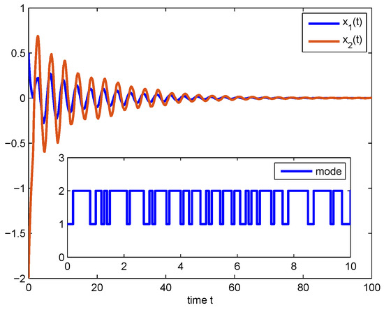
(I) Setting $\Delta A_i=\Delta B_i=\Delta C_i=0$, by using Theorem 1 in [35], the maximum bound of time delays, ${\epsilon }_{max}$, is $1.21$. Using Theorem 1 of the present paper with $\sigma =2$ yields ${\epsilon }_{max}=1.35$. Meanwhile, setting $x\left(0\right)={[0.5,-2]}^{\mathrm{T}}$, the simulations of NS-MJS (1) are plotted in Figure 1. It is seen that NS-MJS (1) with $w\left(t\right)=0$ and $\Delta A_i=\Delta B_i=\Delta C_i=0$ is stochastically stable.

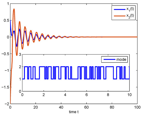
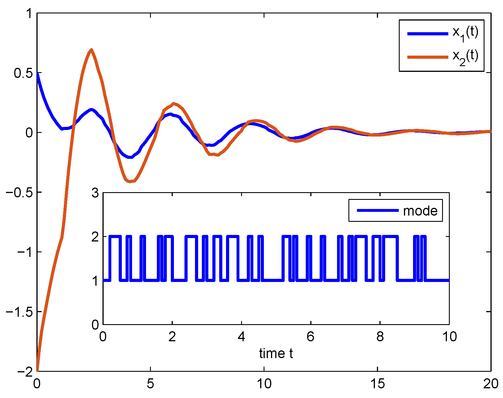
(II) Setting ${\Lambda }_1={\Lambda }_2=I$, $E_{a1}=E_{a2}=E_{b1}=E_{b2}=0.2I$ and $E_{c1}=E_{c2}=0$, by using Theorem 3 in [35], yields ${\epsilon }_{max}=1.05$. Using Theorem 1 from the current paper, when $\sigma =2$, it yields ${\epsilon }_{max}=1.12$. When ${\sigma }_1=2$ and ${\sigma }_2=-0.1$, it yields ${\epsilon }_{max}=1.17$. Moreover, setting $d=1$, using Theorem 1 from the current paper with ${\sigma }_1=2$ and ${\sigma }_2=-0.1$ yields $h_{max}=1.51$. It is said that Theorem 1 is less conservative than that presented in [35], and that the adjustable parameters are efficient. Meanwhile, setting $x\left(0\right)={[0.5,-2]}^{\mathrm{T}}$, ${\Lambda }_2\left(t\right)=cos\left(1.5t\right)$, $\epsilon =1.17$, ${\Lambda }_1\left(t\right)=sin\left(1.5t\right)$, the state responses of uncertain NS-MJSs (1) are plotted in Figure 2. For $d=1$ and $h=1.51$, the state responses of uncertain NS-MJSs (1) are plotted in Figure 3. It is clearly seen in Figure 2 and Figure 3 that uncertain NS-MJSs (1) with $w\left(t\right)=0$ are robustly stochastically stable.

Next, we will test the extended dissipativity performance (EDP) of S-MJS (1) with $w\left(t\right)\ne 0$ as shown in

Table 2. Comparison of EDP performance criteria between the proposed method and Reference [35].

Type	Settings	[35] Results	Proposed Method
$L_2-L_{\infty }$	$\begin{array}{c}{S}_1=0,\hfill \\ S_2=0,\hfill \\ S_3={\gamma }^{2}I,\hfill \\ S_4=0\hfill \end{array}$	${\gamma }_{min}=1.97,d=h=0.3$	${\gamma }_{min}=1.75,{\sigma }_1=2,{\sigma }_2=-0.1$
$H_{\infty }$	$\begin{array}{c}{S}_1=-I,\hfill \\ S_2=0,\hfill \\ S_3={\gamma }^{2}I,\hfill \\ S_4=0\hfill \end{array}$	${\gamma }_{min}=2.33,d=h=0.3$	${\gamma }_{min}=2.07,{\sigma }_1=2,{\sigma }_2=-0.1$
Passivity	$\begin{array}{c}{S}_1=0,\hfill \\ S_2=I,\hfill \\ S_3=\gamma I,\hfill \\ S_4=0\hfill \end{array}$	${\gamma }_{min}=1.25,d=h=0.8$	${\gamma }_{min}=1.07,{\sigma }_1=2,{\sigma }_2=-0.1$
Dissipativity	$\begin{array}{c}{S}_1=-I,\hfill \\ S_2=\left[\begin{array}{cc}1& 0\\ 0.3& 1\end{array}\right],\hfill \\ S_3=3I-\gamma I,\hfill \\ S_4=0\hfill \end{array}$	${\gamma }_{max}=1.19,d=h=0.7$	${\gamma }_{max}=1.54,{\sigma }_1=2,{\sigma }_2=-0.1$

. It was demonstrated from [35] that $L_2-L_{\infty }$, $H_{\infty }$, passivity, and dissipativity can be reduced to EDP by tuning parameters $S_1,S_2,S_3$, and $S_4$. We will analyze the EDP of BS-MJS (1) through the following two cases:

(i) When $\Delta A_i=\Delta B_i=\Delta C_i=0$ and $G_1=G_2=E_1=E_2=F_1=F_2=D_1=D_2=I$, the corresponding performance is shown as follows:

$L_2-L_{\infty }$ performance: For $S_1=0$, $S_2=0$, $S_3={\gamma }^{2}I$, and $S_4=0$, the EDP becomes the $L_2-L_{\infty }$ performance. Setting $d=h=0.3$, making use of Theorem 4 from [35], the minimum $L_2-L_{\infty }$ performance ${\gamma }_{min}$ is $1.63$. By using Theorem 1 of the present paper, when $\sigma =2$, it yields ${\gamma }_{min}=1.34$. When $\sigma =2$, $d=0.3$ and $h=0.5$, it yields ${\gamma }_{min}=1.41$. When ${\sigma }_1=2$, ${\sigma }_2=-0.1$, $d=0.3$, and $h=0.5$, it yields ${\gamma }_{min}=1.34$.

$H_{\infty }$ performance: For $S_1=-I$, $S_2=0$, $S_3={\gamma }^{2}I$, and $S_4=0$, the EDP becomes the $H_{\infty }$ performance. Setting $h=d=0.3$, making use of Theorem 4 from [35], the minimum $L_2-L_{\infty }$ performance ${\gamma }_{min}$ is $2.05$. Using Theorem 1 from the current paper, when $\sigma =2$, it yields ${\gamma }_{min}=1.89$. When $\sigma =2$, $d=0.3$ and $h=0.5$, it yields ${\gamma }_{min}=1.94$. When ${\sigma }_1=2$, ${\sigma }_2=-0.1$, $d=0.3$ and $h=0.5$, it yields ${\gamma }_{min}=1.87$.

Passivity performance: For $S_1=0$, $S_2=I$, $S_3=\gamma I$, and $S_4=0$, the EDP becomes the passivity performance. Making use of Theorem 4 from [35], the minimum passivity performance ${\gamma }_{min}$ is $0.22$. By using Theorem 1 of the present paper, when $\sigma =2$, it yields ${\gamma }_{min}=0.19$. When $\sigma =2$, $d=0.8$ and $h=0.9$, it yields ${\gamma }_{min}=0.29$. When ${\sigma }_1=2$ and ${\sigma }_2=0.1$, $d=0.8$ and $h=0.9$, it yields ${\gamma }_{min}=0.24$.

Dissipativity performance: For $S_1=-I$, $S_2=\left[\begin{array}{cc}1& 0\\ 0.3& 1\end{array}\right]$, $S_3=3I-\gamma I$, and $S_4=0$, the EDP becomes the dissipativity performance. For $h=d=0.7$, making use of Theorem 4 from [35], the maximum dissipativity level ${\gamma }_{max}$ is $1.98$. Using Theorem 1 from the current paper, when $\sigma =2$, it yields ${\gamma }_{max}=2.14$. When $\sigma =2$, $d=0.7$ and $h=0.9$, it yields ${\gamma }_{max}=2.03$. When ${\sigma }_1=2$, ${\sigma }_2=-0.1$, $d=0.7$ and $h=0.9$, it yields ${\gamma }_{max}=2.19$.

(ii) When $\Delta A_i=\Delta B_i=\Delta C_i\ne 0$, choosing ${\Lambda }_1={\Lambda }_2=I$, $E_{a1}=E_{a2}=E_{b1}=E_{b2}=0.2I$, $E_{c1}=E_{c2}=0$ and $G_1=G_2=F_1=F_2=D_1=D_2=E_1=E_2=I$, by setting values of $S_1,S_2,S_3$, $S_4$, the corresponding performance is shown as follows.

$L_2-L_{\infty }$ performance: For $S_1=0$, $S_2=0$, $S_3={\gamma }^{2}I$, and $S_4=0$, the EDP becomes the $L_2-L_{\infty }$ performance. For $h=d=0.3$, the $H_{\infty }$’s minimum performance level (MPL) ${\gamma }_{min}$ in [35] is $1.97$. Using Theorem 1 from the current paper with ${\sigma }_1=2$ and ${\sigma }_2=-0.1$, when $h=d=0.3$, it is ${\gamma }_{min}=1.75$. When $d=0.3$ and $h=0.4$, it is ${\gamma }_{min}=1.81$.

$H_{\infty }$ performance: For $S_1=-I$, $S_2=0$, $S_3={\gamma }^{2}I$, and $S_4=0$, the EDP becomes the $H_{\infty }$ performance. Making use of Theorem 5 from [35], for $h=d=0.3$, the $H_{\infty }$’s MPL ${\gamma }_{min}$ is $2.33$. Using Theorem 1 from the current paper with ${\sigma }_1=2$ and ${\sigma }_2=-0.1$, when $d=h=0.3$, it is ${\gamma }_{min}=2.07$. When $d=0.3$ and $h=0.4$, it is ${\gamma }_{min}=2.16$.

Passivity performance: For $S_1=0$, $S_2=I$, $S_3=\gamma I$, and $S_4=0$, the EDP becomes the passivity. By using Theorem 5 in [35], when $d=h=0.8$, the minimum passivity level ${\gamma }_{min}=1.25$. Using Theorem 1 from the current paper with ${\sigma }_1=2$ and ${\sigma }_2=-0.1$, when $d=h=0.8$, it is ${\gamma }_{min}=1.07$. When $d=0.8$ and $h=0.9$, it is ${\gamma }_{min}=1.14$.

Dissipativity performance: For $S_1=-I$, $S_2=\left[\begin{array}{cc}1& 0\\ 0.3& 1\end{array}\right]$, $S_3=3I-\gamma I$, and $S_4=0$, the EDP becomes the dissipativity. By applying Theorem 5 in [35], when $d=h=0.7$, the maximum dissipativity level ${\gamma }_{max}$ is $1.19$. Using Theorem 1 from the current paper with ${\sigma }_1=2$ and ${\sigma }_2=-0.1$, when $d=h=0.7$, it is ${\gamma }_{max}=1.54$. When $d=0.7$ and $h=0.8$, it is ${\gamma }_{max}=1.37$.

Compared with [35], the proposed extended dissipativity condition is less conservative. Moreover, the adjustable parameters ${\sigma }_1$ and ${\sigma }_2$ are efficient.

5. Conclusions

In this paper, we investigated the extended dissipativity analysis of delayed neural-type systems with semi-Markovian jump parameters. By introducing some adjustable parameters and slack matrices, a PDFSII and a PDFDII were, respectively, proposed, which included some existing inequalities. Less conservative extended-dissipative conditions were achieved for the considered systems through the proposed integral inequalities. The advantages of the obtained conditions were demonstrated using two illustrative examples.

References

- Zeng, H.; He, Y.; Wu, M.; She, J. Free-matrix-based integral inequality for stability analysis of systems with time varying delay. IEEE Trans. Autom. Control 2015, 60, 2768–2772. [Google Scholar] [CrossRef]
- Gu, K.; Kharitonov, V.; Chen, J. Stability of Time-Delay Systems; Birkhauser: Cambridge, MA, USA, 2003. [Google Scholar]
- Seuret, A.; Gouaisbaut, F. Wirtinger-based integral inequality: Application to time-delay systems. Automatica 2013, 49, 2860–2866. [Google Scholar] [CrossRef]
- Zhang, H.; Yan, Y.; Mu, Y.; Ming, Z. Neural Network-Based Adaptive Sliding-Mode Control for Fractional Order Fuzzy System with Unmatched Disturbances and Time-Varying Delays. IEEE Trans. Syst. Man Cybern. Syst. 2023, 53, 5174–5184. [Google Scholar] [CrossRef]
- Tian, Y.; Su, X.; Shen, C.; Ma, X. Exponentially extended dissipativity-based filtering of switched neural networks. Automatica 2024, 161, 111465. [Google Scholar] [CrossRef]
- Zeng, H.; He, Y.; Wu, M.; She, J. New results on stability analysis for systems with discrete distributed delay. Automatica 2015, 60, 189–192. [Google Scholar] [CrossRef]
- He, Y.; Ji, M.; Zhang, C.; Wu, M. Global exponential stability of neural networks with time-varying delay based on free-matrix-based integral inequality. Neural Netw. 2016, 77, 80–86. [Google Scholar] [CrossRef]
- Park, M.; Kwon, O.; Park, J.; Lee, S.; Cha, E. Stability of time delay systems via Wirtinger-based double integral inequality. Automatica 2015, 55, 204–208. [Google Scholar] [CrossRef]
- Zhang, B.; Zheng, W.; Xu, S. Filtering of Markovian jump delay systems based on a new performance index. IEEE Trans. Circuits Syst. I 2013, 60, 1250–1263. [Google Scholar] [CrossRef]
- Li, F.; Wu, L.; Shi, P. Stochastic stability of semi-Markovian jump systems with mode-dependent delays. Int. J. Robust Nonlinear Control 2014, 24, 3317–3330. [Google Scholar] [CrossRef]
- Hua, C.; Wu, S.; Yang, X.; Guan, X. Stability analysis of time-delay systems via free-matrix-based double integral inequality. Int. J. Syst. Sci. 2017, 48, 257–263. [Google Scholar] [CrossRef]
- Saravanakumar, R.; Rajchakit, G.; Ahn, C.K.; Karimi, H.R. Exponential Stability, Passivity, and Dissipativity Analysis of Generalized Neural Networks with Mixed Time-Varying Delays. IEEE Trans. Syst. Man Cybern. Syst. 2019, 49, 395–405. [Google Scholar] [CrossRef]
- Xiong, L.; Cheng, J.; Liu, X.; Wu, T. Improved conditions for neutral delay systems with novel inequalities. J. Nonlinear Sci. Appl. 2017, 10, 2309–2317. [Google Scholar] [CrossRef]
- Ali, M.S.; Narayanan, G.; Nahavandi, S.; Wang, J.-L.; Cao, J. Global Dissipativity Analysis and Stability Analysis for Fractional-Order Quaternion-Valued Neural Networks with Time Delays. IEEE Trans. Syst. Man Cybern. Syst. 2022, 52, 4046–4056. [Google Scholar] [CrossRef]
- Faydasicok, O. New criteria for global stability of neutral-type Cohen-Grossberg neural networks with multiple delays. Neural Netw. 2017, 48, 257–263. [Google Scholar] [CrossRef]
- Arik, S. New criteria for stability of neutral-type neural networks with multiple time delays. IEEE Trans. Neural Netw. Learn. Syst. 2020, 15, 1504–1513. [Google Scholar] [CrossRef]
- Tian, Y.; Wang, Z. Extended dissipativity analysis for Markovian jump neural networks via double integral-based delay-product-type Lyapunov functional. IEEE Trans. Neural Netw. Learn. Syst. 2022, 32, 3240–3246. [Google Scholar] [CrossRef]
- Tian, Y.; Wang, Z. Finite-time extended dissipative filtering for singular T-S fuzzy systems with nonhomogeneous Markov jumps. IEEE Trans. Cybern. 2022, 52, 4574–4584. [Google Scholar] [CrossRef]
- Zhang, Y.; Lou, K.; Ge, Y. New Result on delay-dependent stability for Markovian jump time-delay systems with partial information on transition probabilities. IEEE/CAA J. Autom. Sin. 2019, 6, 1499–1505. [Google Scholar] [CrossRef]
- Dong, S.; Chen, C.L.; Fang, M.; Wu, Z. Dissipativity-based asynchronous fuzzy sliding mode control for T-S fuzzy hidden Markov jump systems. IEEE Trans. Cybern. 2019, 50, 4020–4030. [Google Scholar] [CrossRef]
- Fu, L.; Ma, Y.; Wang, C. Memory sliding mode control for semi-Markov jump system with quantization via singular system strategy. Int. J. Robust Nonlinear Control 2019, 29, 6555–6571. [Google Scholar] [CrossRef]
- Zong, G.; Ren, H. Guaranteed cost finite-time control for semi-Markov jump systems with event-triggered scheme and quantization input. Int. J. Robust Nonlinear Control 2019, 29, 5251–5273. [Google Scholar] [CrossRef]
- Yao, L.; Wang, Z.; Huang, X.; Li, Y.; Ma, Q.; Shen, H. Stochastic Sampled-Data Exponential Synchronization of Markovian Jump Neural Networks with Time-Varying Delays. IEEE Trans. Neural Netw. Learn. Syst. 2023, 34, 909–920. [Google Scholar] [CrossRef] [PubMed]
- Zhang, H.; Yan, Y.; Sun, J. A-Iterative Dual Heuristic Dynamic Programming for Nonlinear Critical Surfaces with Strong Constraints. IEEE Trans. Syst. Man Cybern. Syst. 2024, 54, 3334–3343. [Google Scholar] [CrossRef]
- Subramaniam, S.; Lim, C.P.; Rajan, R.; Mani, P. Synchronization of Fractional Stochastic Neural Networks: An Event Triggered Control Approach. IEEE Trans. Syst. Man Cybern. Syst. 2024, 54, 1113–1123. [Google Scholar] [CrossRef]
- Xu, Y.; Wu, Z.; Pan, Y.; Sun, J. Resilient Asynchronous State Estimation for Markovian Jump Neural Networks Subject to Stochastic Nonlinearities and Sensor Saturations. IEEE Trans. Cybern. 2022, 52, 5809–5818. [Google Scholar] [CrossRef]
- Wang, J.; Ma, S.; Zhang, C. Resilient estimation for T-S fuzzy descriptor systems with semi-Markov jumps and time-varying delay. Inf. Sci. 2018, 430, 104–126. [Google Scholar] [CrossRef]
- Yin, G.; Krishnamurthy, V.; Ion, C. Regime switching stochastic approximation algorithms with application to adaptive discrete stochastic optimization. SIAM J. Optim. 2004, 14, 1187–1215. [Google Scholar] [CrossRef]
- Huang, J.; Shi, Y.; Zhang, X. Active fault tolerant control systems by the semi-Markov model approach. Int. J. Adapt. Control Signal Process. 2014, 28, 833–847. [Google Scholar] [CrossRef]
- Xu, Z.; Wu, Z.; Su, H.; Shi, P.; Que, H. Energy-to-peak filtering of semi-markov jump systems with mismatched modes. IEEE Trans. Autom. Control 2020, 65, 4356–4361. [Google Scholar] [CrossRef]
- Shen, H.; Wu, Z.; Park, J. Reliable mixed passive and H∞ filtering for semi-Markov jump systems with randomly occurring uncertainties and sensor failures. Int. J. Robust Nonlinear Control 2015, 25, 3231–3251. [Google Scholar] [CrossRef]
- Xia, W.; Xu, S.; Ma, Q.; Qi, Z.; Zhang, Z. Dissipative controller design for uncertain neutral systems with semi-Markovian jumping parameters. Optim. Control Appl. Meth. 2018, 39, 888–903. [Google Scholar] [CrossRef]
- Sakthivel, R.; Kwon, O.; Choi, S.; Sakthivel, R. Observer-based state estimation for discrete-time semi-Markovian jump neural networks with round-robin protocol against cyber attacks. Neural Netw. 2023, 165, 611–624. [Google Scholar] [CrossRef] [PubMed]
- Sakthivel, R.; Sakthivel, R.; Kwon, O.; Selvaraj, P. Disturbance rejection for singular semi-Markov jump neural networks with input saturation. Appl. Math. Comput. 2021, 407, 126301. [Google Scholar] [CrossRef]
- Wu, T.; Xiong, L.; Cao, J.; Zhang, H. Stochastic stability and extended dissipativity analysis for uncertain neutral systems with semi-Markovian jumping parameters via novel free matrix-based integral inequality. Int. J. Robust Nonlinear Control 2019, 29, 2525–2545. [Google Scholar] [CrossRef]
- Liang, X.L.; Hou, M.Z.; Duan, G.R. Output feedback stabilization of switched stochastic nonlinear systems under arbitrary switchings. Int. J. Autom. Comput. 2013, 10, 571–577. [Google Scholar] [CrossRef]
- Wang, D.; Wu, F.; Lian, J.; Li, S. Observer-based asynchronous control for stochastic nonhomogeneous semi-Markov jump systems. IEEE Trans. Autom. Control 2023, 69, 2559–2566. [Google Scholar] [CrossRef]
Disclaimer/Publisher’s Note: The statements, opinions and data contained in all publications are solely those of the individual author(s) and contributor(s) and not of MDPI and/or the editor(s). MDPI and/or the editor(s) disclaim responsibility for any injury to people or property resulting from any ideas, methods, instructions or products referred to in the content. |
© 2025 by the authors. Licensee MDPI, Basel, Switzerland. This article is an open access article distributed under the terms and conditions of the Creative Commons Attribution (CC BY) license (https://creativecommons.org/licenses/by/4.0/).