Dynamic Error Compensation for Ball Screw Feed Drive Systems Based on Prediction Model

Abstract

The dynamic error is the dominant factor affecting multi-axis CNC machining accuracy. Predicting and compensating for dynamic errors is vital in high-speed machining. This paper proposes a novel prediction-model-based approach to predict and compensate for the ball screw feed system’s dynamic error. Based on the lumped and distributed mass methods, this method constructs a parameterized dynamic model relying on the moving component’s position for electromechanical coupling modeling. Using Latin Hypercube Sampling and numerical simulation, a sample set containing the input and output of one control cycle is obtained, which is used to train a Cascade-Forward Neural Network to predict dynamic errors. Finally, a feedforward compensation strategy based on the prediction model is proposed to improve tracking performance. The proposed method is applied to a ball screw feed system. Tracking error simulations and experiments are conducted and compared with the transfer function feedforward compensation. Typical trajectories are designed to validate the effectiveness of the electromechanical coupling model, the dynamic error prediction model, and the feedforward compensation strategy. The results show that the prediction model exhibits a maximum prediction deviation of 1.8% for the maximum tracking error and 13% for the average tracking error. The proposed compensation method with friction compensation achieves a maximum reduction rate of 76.7% for the maximum tracking error and 63.7% for the average tracking error.

1. Introduction

A ball screw feed system is composed of rotary motors, linear guides, and ball screws, functioning together to transform the motor’s rotational motion into precise linear displacement along the guide rail. Ball screws demonstrate high efficiency, extended service life, superior load-bearing capacity, excellent stiffness, long travel ranges, and minimal heat generation, enabling consistent acceleration performance even under significant variations in workpiece inertia. Multiple technical parameters collectively affect feed system accuracy–mechanical vibration in screw drives, control system design, environmental noise, and sensor resolution all contribute to final positioning results. Monitoring and compensating for tracking errors in ball screw feed systems facilitates error reduction and accuracy enhancement.

The prerequisite for dynamic error prediction and compensation is establishing an accurate electromechanical coupling model that accounts for positional variations. Numerous simulation and experimental studies confirm that ball screw feed drives display substantial dynamic behavior variations correlated with position, stemming mainly from changes in the active screw length during motor–worktable displacement. This phenomenon results in position-dependent dynamic behavior during system operation. Current approaches for developing position-dependent dynamic models include dictionary function libraries [1], observer-based methods [2], and linear parameter-varying (LPV) techniques [3]. These position-dependent characteristics substantially influence motion control precision. Integrating worktable position effects into motion control strategies can significantly improve dynamic tracking accuracy.

Constructing dynamic models for ball screw feed systems represents a fundamental aspect of studying their dynamic characteristics. An accurate dynamic model provides theoretical foundations for analyzing system dynamic behavior and establishes a critical technical foundation for digital design and simulation, dynamic optimization design, and dynamic error modeling and control. Existing mainstream modeling strategies encompass lumped parameter models [4,5,6,7], distributed parameter frameworks [6,7], and finite element-based techniques [8,9,10]. The lumped mass method has been widely adopted due to its computational efficiency and low resource requirements. However, its limitations include potential inaccuracies in capturing mass distribution effects on structural dynamic responses, which may compromise model prediction accuracy under certain operating conditions. In comparison, the distributed mass method facilitates the construction of more precise dynamic models, albeit with substantially increased computational complexity. While the finite element method offers superior modeling accuracy, its computational resource requirements significantly exceed those of the other techniques, consequently limiting its practical engineering applications to some extent.

Dynamic error modeling forms the theoretical foundation for dynamic error prediction and compensation research, where the rationality of the model architecture directly determines the scientific validity and reliability of related studies. Based on the diversity of modeling principles, existing dynamic error modeling approaches can be systematically categorized into three main classes: analytical modeling based on dynamic systems, statistical modeling based on characteristic parameters, and mechanism modeling based on generation principles. The dynamics-based modeling method utilizing system transfer functions achieves error characterization by establishing mathematical relationships between control elements [11,12]. While this method demonstrates computational efficiency advantages, its prediction accuracy is inherently limited by model simplification assumptions. In contrast, the integrated modeling approach based on multi-physics coupling incorporates servo control and mechanical structure models through commercial simulation platforms [13,14]. The improved accuracy comes at the expense of computational burden, revealing the intrinsic conflict between model precision and processing efficiency. Under the data-driven modeling paradigm, characteristic parameter-based dynamic error modeling reconstructs errors by extracting feature parameters from measurement signals and establishing parametric functional relationships [15,16]. Notably, the multi-source nature of dynamic error generation mechanisms induces prevalent multi-band coupling phenomena in measured signals, significantly challenging the identification accuracy of characteristic parameters. The mechanism-based modeling approach follows a methodology combining mechanism decomposition and linear superposition: first analyzing error generation mechanisms, then quantifying operational patterns of key influencing factors, and ultimately constructing system-level error models [17,18]. Although this approach demonstrates strong physical interpretability, current research still faces two critical limitations: (1) incomplete theoretical descriptions of dynamic error generation mechanisms and (2) unestablished quantitative mapping relationships between influencing factors and resultant error patterns. These limitations constitute fundamental bottlenecks hindering the engineering implementation of this methodology.

Current error compensation strategies can be classified into offline pre-compensation [19,20] and online feedforward compensation [21,22]. Feedforward compensation methods exhibit superior computational efficiency and require minimal modifications to the original control system architecture, making them highly valuable for practical engineering applications.

The tracking accuracy of ball screw feed systems is significantly influenced by friction, and their tracking performance can be further enhanced through friction compensation. The LuGre model [23] integrates key features of the Coulomb, Stribeck, and viscous friction models while incorporating frictional hysteresis. Notably, it retains the state variable z from the Dahl model to describe pre-sliding dynamics. It simplifies the complexity of the Bristle model, thereby offering greater engineering applicability due to its structural simplicity and ease of implementation.

The accuracy of the dynamics-based modeling method improved with computational burden growth. The accuracy of the characteristic parameter-based dynamic error modeling method depends on the identification accuracy of characteristic parameters. The mechanism-based modeling approach’s accuracy relies on complete theoretical descriptions of dynamic error generation mechanisms and established quantitative mapping relationships between influencing factors and resultant error. Considering the disadvantages of these methods, the Cascade-Forward Neural Network (CFNN) prediction model was proposed to describe dynamic error with high precision and low computational burden. With adequate sample points, CFNN can quantitatively map relationships between influencing factors and resultant responses without identifying characteristic parameters. To obtain samples, a dynamic modeling framework that accounts for coupled rigid–flexible interactions in ball screw feed drives with explicit consideration of moving element positioning is formulated. The computational efficiency and accuracy are balanced by integrating the lumped and distributed mass methods. An electromechanical coupling model is developed based on this foundation. The sampling space was populated using Latin Hypercube Sampling (LHS) techniques, with generated parameter combinations serving as inputs to the coupled electromechanical simulation model. These samples train a CFNN prediction model to predict worktable position and dynamic error within a single control cycle, comprehensively accounting for position variation and friction effects. With sufficient sample points, the prediction model achieves high-fidelity emulation of the original system behavior while substantially reducing computational demands. At the start of each control cycle, the dynamic error is calculated by subtracting the predicted worktable position from the reference position. The predicted dynamic error is compensated to the position loop for reducing real-time tracking errors, effectively improving motion accuracy. The main contributions of this work are as follows:

(1) A dynamic modeling method relying on moving components’ positions is proposed based on the lumped and distributed mass methods. The resulting coupled electromechanical system model is systematically validated via simulations and experiments.

(2) Based on the proposed electromechanical coupling model and LHS, a prediction model is constructed to predict the table position and dynamic error within a single control cycle.

(3) The ball screw feed system’s dynamic error is compensated by applied the constructed prediction model and a friction model.

(4) The methodological effectiveness is substantiated through comprehensive testing, incorporating both computational simulations and physical experiments performed on a purpose-built ball screw feed system platform.

The remainder of this paper is organized as follows. Section 2 describes the methodology of dynamic error prediction and feedforward compensation. Section 3 details the electromechanical coupling modeling process. Section 4 systematically presents the dynamic error modeling process and feedforward compensation strategy. Section 5 describes the simulations and experiments. Finally, Section 6 provides conclusions and discusses future work.

2. Methodology

The schematic representation of the methodological framework is presented in Figure 1. To begin with, a position-dependent dynamic model was established based on the distributed mass method and lumped mass method. Combined with Field-Oriented Control (FOC), an electromechanical coupling model of the ball screw feed system was developed. Subsequently, input parameters and design space were determined. Different input combinations were obtained through the LHS experiment design. Numerical simulations using the electromechanical coupling model and the input combinations generated sample points. These sample points were then employed to train a CFNN for dynamic error prediction. Following this, a feedforward compensation strategy was proposed based on the dynamic error prediction model. Finally, experimental validation was conducted to verify the accuracy of the dynamic error prediction model and the effectiveness of the dynamic error compensation strategy.

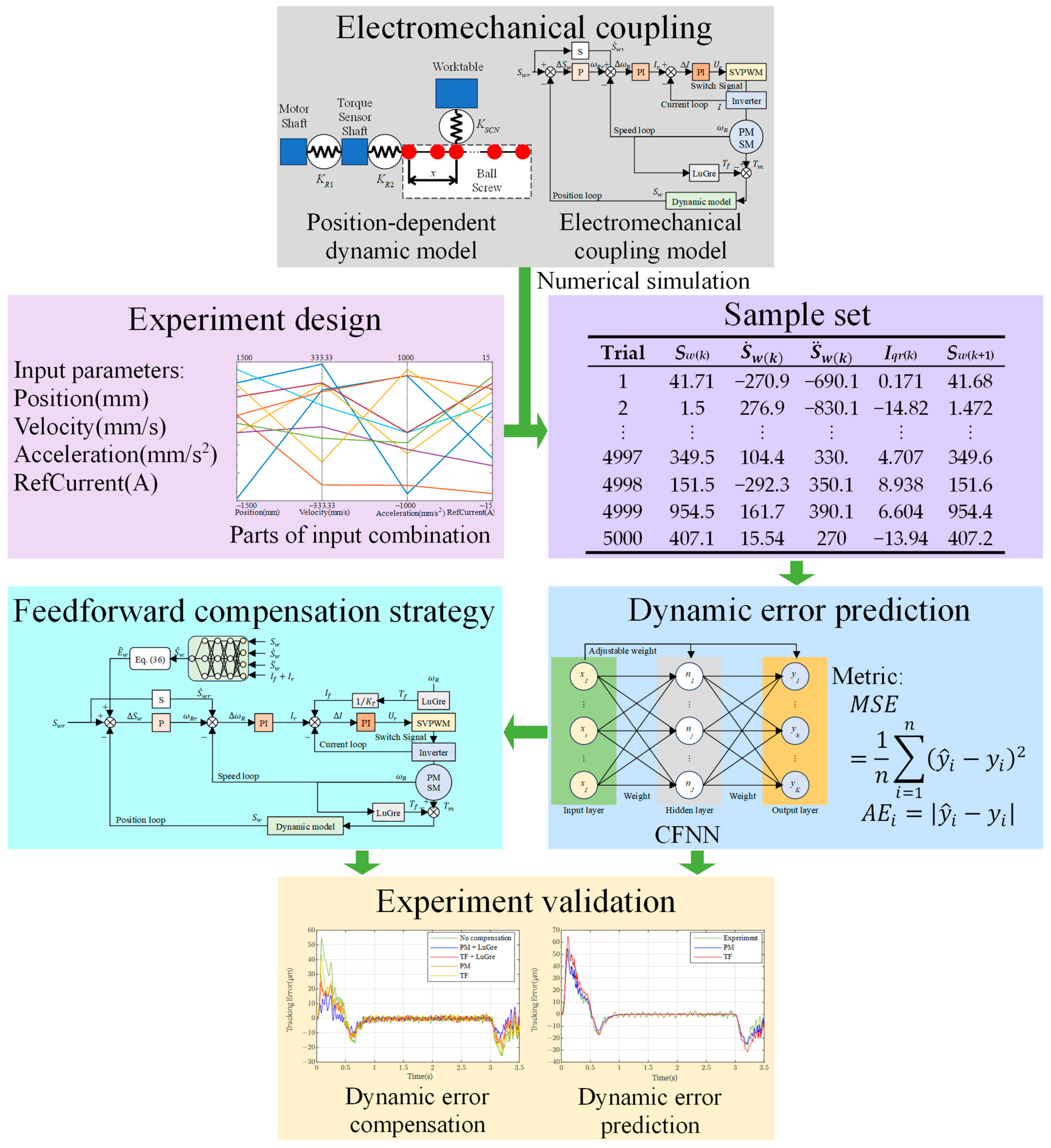
3. Electromechanical Coupling Model of the Ball Screw Feed System

In this section, two complementary mass modeling methods–lumped and distributed–are combined in this section to formulate a dynamic model with explicit position dependency for ball screw feed systems. Subsequently, the system’s friction is identified based on the LuGre model. Finally, an electromechanical coupling model is developed through FOC.

3.1. Position-Dependent Dynamics Modeling Based on the Lumped Mass Method and Distributed Mass Method

3.1.1. Lumped Mass Model of Two Shafts and Worktable

Figure 2a displays the ball screw feed system’s configuration. Figure 2b is a real ball screw feed system. The bed, the permanent magnet synchronous motor (PMSM), the couplings, the torque sensor, the bearings, the bearing housings, the nut, the guide rails, the sliders, the ball screw, and the worktable. Components with relatively small deformations in the ball screw feed system are treated as lumped masses to balance computational efficiency and accuracy, including the shaft of the PMSM, the shaft of the torque sensor, and the worktable, numbered sequentially as 1, 2, and 3. The bed, bearing housings, and guide rails are neglected and have minimal influence on axial motion. The ball screw, which exhibits relatively high flexibility, is modeled using the Timoshenko beam theory [24] to establish a distributed mass dynamic model in Section 3.1.2. The generalized coordinates for lumped masses 1–3 are denoted as q₁, q₂, and q₃, where q₁ and q₂ represent the rotation of lumped masses 1 and 2, respectively, and q3 represents the translation of lumped mass 3.

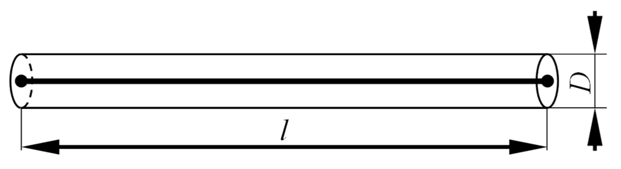
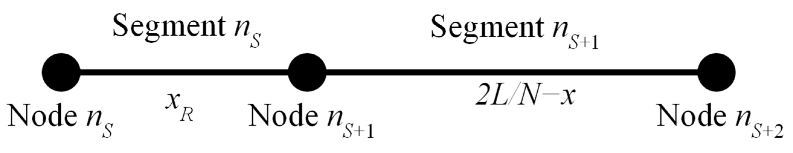
3.1.2. Position-Dependent Distributed Mass of the Screw

The screw shaft in ball screw feed mechanisms exhibits substantial elastic deformation characteristics, necessitating the adoption of Timoshenko beam theory [24] for developing a distributed-parameter dynamic model. The calculation of Timoshenko beam element matrices can be found in the Appendix A. Based on the principles underlying the derivation of the Timoshenko beam element matrices, a distributed mass model related to the position of the lead screw is established. Define L as the total screw length divided into N discrete segments. When the axial displacement between drive and load interfaces is x, the output position resides in segment n_S:

$$n_S=⌈{\displaystyle \frac{N}{L}}x⌉$$

(1)

where ⌈⋅⌉ denotes the ceiling function. The remaining length x_R falls within the n_S-th segment. The remaining dimension x_R is positioned within the n_S-th section. Through modification of these two adjacent segments, the n_S-th section’s length becomes equal to x_R. The subsequent segment (n_S+1) length, denoted as l_ns+1, can be determined using Equation (2). This adjusted n_S+1 node subsequently functions as the lead screw’s output terminal, with the modified configuration visually represented in Figure 3. The remaining portion of the lead screw is modeled as a conventional Timoshenko beam. Therefore, both the stiffness and mass distribution matrices characterizing the lead screw system exhibit (6N + 6) × (6N + 6) dimensionality, where all constituent elements dynamically depend on the spatial coordinate x.

$$l_{n_{S+1}}=2{\displaystyle \frac{L}{N}}-x_R$$

(2)

3.1.3. Position-Dependent Dynamic Model of Ball Screw Feed System

The matrix elements about the RX-direction DOF are extracted to derive the screw’s RX-direction distributed mass stiffness matrix K_RX and mass matrix M_RX based on the distributed mass model presented in Section 3.1.2. These matrices’ dimensions are (N + 1) × (N + 1). The model of joints must also be established with the lumped masses described in Section 3.1.1. Based on the lumped mass assumption in Section 3.1.1, Lumped Mass 1 and Lumped Mass 2 are connected by a single degree of freedom (SDOF) spring K_R1, representing rotational stiffness along the RX-direction, with a magnitude equal to the rotational stiffness of the shaft coupling between the motor shaft and the torque sensor. Similarly, Lumped Mass 2 and the screw input end are connected by an SDOF spring K_R2, corresponding to rotational stiffness along the RX-direction, with a magnitude equal to the rotational stiffness of the shaft coupling between the torque sensor and the screw. According to [25], the ball screw nut generates axial thrust simultaneously with torque. The functional dependence of axial thrust F on torque T_n is mathematically defined through Equation (3):

$$T_n=FR\tan \varphi$$

(3)

where R is the screw radius and ϕ is the screw contact angle. Let the generalized coordinate vector between the screw output end and Lumped Mass 3 be defined as Q_scn = [q_scnRx q_wt], where q_scnRx represents the degree of freedom of the screw output end along the RX-direction, and q_wt is the worktable DOF along the X-direction. The corresponding screw–nut pair’s stiffness matrix K_scn is then given by

$$K_{scn}=\left[\begin{array}{cc}{\displaystyle \frac{r_{scn}{l}_{lead}\tan (\varphi )}{2\pi }}& -r_{scn}\tan (\varphi )\\ -{\displaystyle \frac{l_{lead}}{2\pi }}& 1\end{array}\right]k_{scn}$$

(4)

where r_scn is the screw radius, l_lead is the lead of the screw, and k_scn is the axial stiffness of the screw–nut pair. Let the ball screw feed system’s mass matrix M and stiffness matrix K be matrices of size (N + 4) × (N + 4). The stiffness matrix K’s elements are defined as follows:

$$K(1,1)=-K(2,1)=-K(1,2)=K_{R1}$$

(5)

$$K(2,2)=K_{R1}+K_{R2}$$

(6)

$$K(2,3)=K(3,2)=-K_{R2}$$

(7)

$$K(3,3)=K_{R2}$$

(8)

$$K(n_S+1,n_S+1)=K_{snc}(1,1)$$

(9)

$$K(n_S+1,N+4)=K_{snc}(1,2)$$

(10)

$$K(N+4,n_S+1)=K_{snc}(2,1)$$

(11)

$$K(N+4,N+4)=K_{snc}(2,2)$$

(12)

All other elements are set to zero. Based on this framework, the elements of K_RX are added to the corresponding positions of the submatrix K [{3, N + 3}, {3, N + 3}], thereby obtaining the position-dependent stiffness matrix K(x) associated with the coordinate x. The mass matrix M’s elements are defined as follows:

$$M(1,1)=j_m$$

(13)

$$M(2,2)=j_{TS}$$

(14)

$$M(N+4,N+4)=m_{wt}$$

(15)

All other elements are set to zero. Based on this framework, the elements of MRX are added to the corresponding positions of the submatrix M [{3, N + 3}, {3, N + 3}], thereby obtaining the position-dependent mass matrix M(x) associated with the coordinate x. The ball screw feed system’s position-dependent dynamic model is expressed as follows:

$$M(x)\ddot{Q}+K(x)Q=F$$

(16)

Here, Q corresponds to the node-level generalized displacement vector, while F signifies the per-node force components. The ball screw feed system’s position-dependent dynamic model is illustrated in Figure 4.

3.2. Friction Identification Based on the LuGre Model

The LuGre model constitutes a generalized friction modeling framework incorporating the Stribeck effect, Coulomb friction, and static friction maxima, enabling precise characterization of both gross sliding regimes and pre-sliding. This model quantifies frictional disturbances through elastic bristle deflection: microscopic bristles (modeled as damped springs) undergo pseudo-deflection, whose temporal evolution generates frictional torque. The equations are expressed as

$$T_f={\sigma }_{0}z+{\sigma }_1{\displaystyle \frac{dz}{dt}}+{\sigma }_2\omega$$

(17)

$${\displaystyle \frac{dz}{dt}}=\omega -{\displaystyle \frac{\left|\omega \right|}{g(\omega )}}z$$

(18)

$${\sigma }_{0}g\left(w\right)=T_C+\left(T_S-T_C\right)e^{-{\left({\displaystyle \frac{\omega }{{\Omega }_S}}\right)}^2}$$

(19)

where ω denotes the angular speed, z denotes the bristle deformation, σ₀ is the bristle stiffness coefficient, σ₁ corresponds to the bristle damping coefficient, σ₂ signifies the viscous friction coefficient, Ω_S represents the critical Stribeck velocity, T_C denotes the Coulomb friction torque, and T_S represents the maximum static friction torque. The LuGre model requires identifying six parameters, including four static and two dynamic parameters. In ball screw feed systems, friction primarily occurs at the motion–contact interfaces. A systematic friction identification methodology was employed, with constant-velocity experiments specifically designed. When the system operates at a constant velocity, the system acceleration becomes zero. According to Newton’s second law,

$$T_m=m_e{a}_e+T_f$$

(20)

Here, T_m denotes the motor output torque, me corresponds to the system’s equivalent inertia, and ae represents the system’s equivalent acceleration. Consequently, T_m equals T_f. The identification results are presented in

Table 1. Identification results.

Parameters	TC (N·mm)	TS (N·mm)	ΩS (rpm)	σ0(N)	σ1 (N·mm/rpm)	σ2 (N·mm/rpm)
value	0.6757	0.7653	25.9147	1.5875	0.1593	0.0003

.

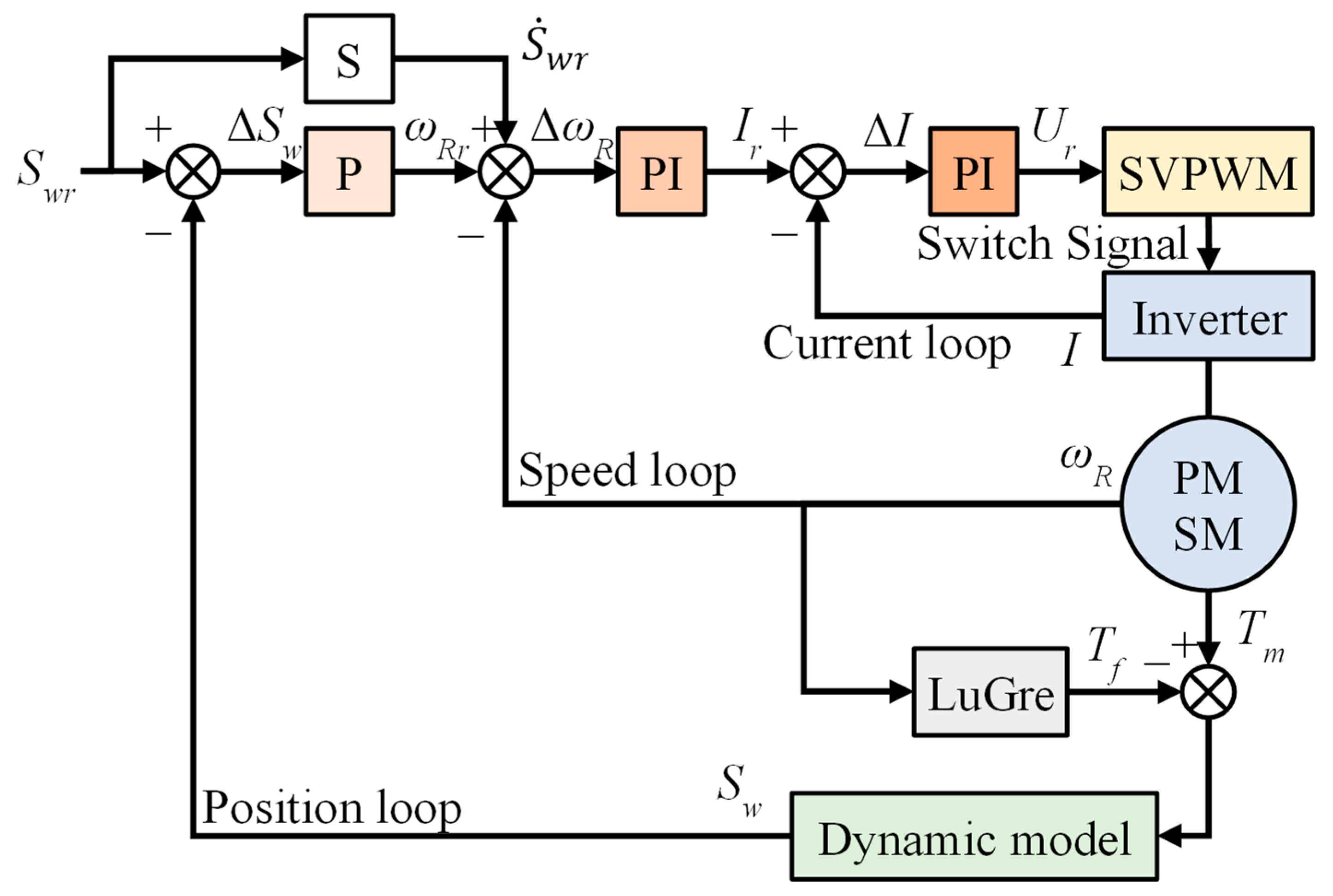
3.3. Electromechanical Coupling Modeling of the Ball Screw Feed System

The electromechanical coupling model based on FOC is constructed using the dynamic model proposed in Section 3.1. The core of FOC lies in its approach, akin to that of DC motor control, utilizing coordinate transformation theory to decouple the armature current and excitation current in a PMSM into two independent components for individual control. FOC methods primarily include maximum output power control method, maximum torque/current control method, field weakening control method, the I_d = 0 control method, and transverse flux linkage control method, depending on the application. The I_d = 0 control method is employed to regulate the PMSM [26].

The electromechanical coupling model is illustrated in Figure 5. The input to the electromechanical coupling model is the reference table position S_wr. As shown in Figure 5, S_w denotes the table position, ΔS_w represents the tracking error, ω_Rr is the reference velocity, ω_R is the actual motor velocity, Δω_R is the velocity error, I_r is the reference current, I is the actual current, ΔI is the current error, and U_r is the reference voltage. By employing space vector pulse width modulation (SVPWM), U_r is input to the PMSM to generate torque T_m. SVPWM further smoothens the motor’s output torque [27]. The LuGre model provides the friction force T_f. S_w is the generalized coordinate of the worktable’s lumped mass along the y-axis.

The operational specifications of the PMSM and the ball screw feed mechanism are in

Table 2. The operational specifications of the PMSM.

Operational Specifications	Value
Rotor inertia	0.0053 (kg·m2)
Torque constant	1.641 (N·m/A)
Stator resistance	0.75 (ohm)
The inductance of the quadrature axis	13.2 (mH)
The inductance of the direct axis	4.11 (mH)
Rated torque	24 (N·m)
Rated current	10 (A)
Rated speed	2000 (RPM)
Coil pitch	4
Silicon steel grades	M270-35A
Permanent magnet grades	N42UH

and

Table 3. The operational specifications of the ball screw feed system.

Operational Specifications	Value
Ball screw manufacturer	HIWIN
Ball screw catalog	FDI 40-10T3
Bed material grade	HT200
Worktable material grade	HT200
Rotary table material grade	QT450-10
Torque sensor shaft stiffness	1 × 105 (N·m/rad)
Coupling torsional stiffness	2800 (N·m/rad)
Screw–nut pair axial stiffness	7.45 × 107 (N/m) 1.04 × 107 (N/m)

, respectively. Controller gains for the PI and P regulators were optimized following methodologies in [28]. Position–velocity control loop parameters, designated as P_Sw, P_ωR, and I_ωR, govern the motion tracking dynamics, while current regulation in the rotating reference frame is implemented through q- and d-axis PI coefficients P_iq, I_iq, P_id, and I_id, as detailed in

Table 4. Control parameters.

PId	IId	PIq	IIq	PωR	IωR	PSw
2.776	626.2	8.805	1003.3	0.0678	0.7122	280.2

. A 10 kHz sampling rate was implemented throughout the experimental framework, with inverter dead-time effects and viscous damping forces intentionally excluded from the system modeling.

4. Dynamic Error Modeling of One Control Cycle and Feedforward Compensation

This section presents the specific workflow of the dynamic error feedforward compensation method based on the prediction model. First, the fundamental principles are elaborated. Subsequently, sample points are generated through LHS combined with an electromechanical coupling model of the ball screw feed system. These sample points are then utilized to train a CFNN-based prediction model. Finally, the prediction model feedforward compensation is proposed for the dynamic error.

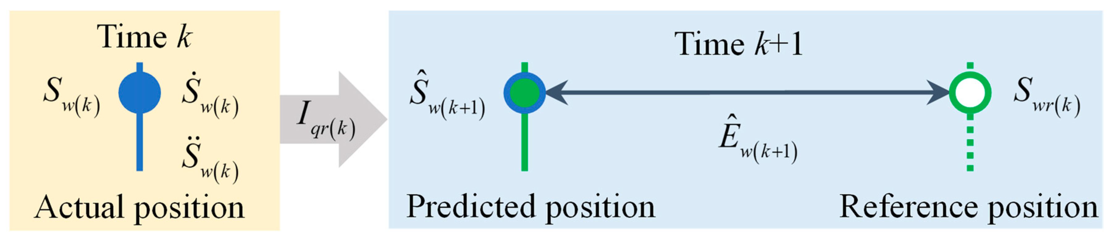
4.1. Basic Principles and Processes

Assuming the feed system is at time point k, the position of the workbench is S_w(k), and the velocity is ${\dot{S}}_{w\left(k\right)}$ The acceleration is ${\ddot{S}}_{w\left(k\right)}$, and the motor’s reference q-axis current command is I_qr(k). Under the command of I_qr(k), the motor drives the feed system to operate. At time point k + 1, the position of the workbench is S_w(k+1), as shown in Figure 6.

4.2. Latin Hypercube Sampling Experimental Design

LHS is a widely utilized experimental design method in computer simulations. Compared with classical Monte Carlo sampling approaches, which tend to produce clustered sample distributions, LHS optimizes Monte Carlo sampling by ensuring more uniform and efficient sampling across the design space of multiple variables. The fundamental principle of LHS parallels stratified sampling, incorporating both stratification and random permutation. The procedure of LHS is described here. Let (v₁, v₂, …, v_m) represent m input variables, where the range of v_j is defined as R_j = [A_j, B_j] for j = 1, 2, …, m. The cumulative distribution function of v_j is denoted as V = G(v_j), as documented in reference [29].

Step 1: Partition R_j into n stratified intervals, denoted as R_j1, R_j2, …, R_jn, each possessing equal probability. These subdivisions satisfy the following conditions:

$$\left\{\begin{array}{l}{R}_{j1}\cup R_{j2}\cup \dots \cup R_{jm}\\ R_{jk}\cap R_{jl}=\varnothing \end{array}\right.$$

(21)

$$P(v_j\in R_{jk})={\displaystyle \frac{1}{n}}(k,l=1,2\dots ,n)$$

(22)

Step 2: The cumulative probability value of the input variable v_j for the k-th interval is derived via Equation (23):

$$G\left(v_j\in R_{jk}\right)={\displaystyle \frac{k-1}{n}}+{\displaystyle \frac{u_{jk}}{n}},u_{jk}\sim U(0,1)$$

(23)

Here, u_jk constitutes a stochastic variable following uniform distribution across the unit interval [0, 1]. The cumulative probabilities of the input variables (v₁, v₂, …, v_m) can be formalized as an n×m matrix Q = (P_kj)_n×m, where P_kj is the cumulative probability value associated with the k-th stratified interval of the j-th variable.

Step 3: Utilizing the inverse function of G (·), the probability values from Equation (23) are transformed into sampled values v_kj, as expressed in Equation (24):

$$G\left(v_j\in R_{jk}\right)={\displaystyle \frac{k-1}{n}}+{\displaystyle \frac{u_{jk}}{n}},u_{jk}\sim U(0,1)$$

(24)

The sample matrix V can be derived.

$$V=\left[\begin{array}{cccc}{v}_{11}& v_{12}& \dots & v_{1m}\\ v_{21}& v_{22}& \dots & v_{2m}\\ ⋮& ⋮& \ddots & ⋮\\ v_{n1}& v_{n2}& \dots & v_{nm}\end{array}\right]$$

(25)

Step 4: Randomly combine the variables into n sampling groups as follows:

$$V^{\prime }=\left[\begin{array}{cccc}{v}_{11}^{\prime }& v_{12}^{\prime }& ⋮& v_{1m}^{\prime }\\ v_{21}^{\prime }& v_{22}^{\prime }& ⋮& v_{2m}^{\prime }\\ \dots & \dots & \ddots & ⋮\\ v_{n1}^{\prime }& v_{n2}^{\prime }& ⋮& v_{nm}^{\prime }\end{array}\right]={\left(v_{1m}^{\prime },v_{2m}^{\prime },\dots ,v_{nm}^{\prime }\right)}^T$$

(26)

Each row within the matrix encapsulates a distinct grouping of spatial or temporal sampling coordinates, reflecting the structured organization of collected data points. The design space comprises S_w(k), ${\dot{S}}_{w\left(k\right)}$, ${\ddot{S}}_{w\left(k\right)}$, and I_qr(k). The ball screw has a length of 0–1500 mm; consequently, the worktable position S_w(k) is constrained within the range of 0–1500 mm. ${\dot{S}}_{w\left(k\right)}$ directly correlates with the motor’s nominal angular velocity of 2000 RPM. Given the ball screw lead of 10 mm, the range of ${\dot{S}}_{w\left(k\right)}$ is determined to be −333 to 333 mm/s. The motor’s rated current is 10 A, and considering that the equivalent current equals 0.707 times the instantaneous current, the range of I_qr(k) is set to −15 A to 15 A. With a worktable mass of 515 kg and a maximum acceleration capability of 30,000 mm/s², the stator current may trigger the motor driver’s overcurrent protection when the initial acceleration reaches 4000 mm/s². Therefore, accounting for the acceleration characteristics of the S-shaped velocity profile, the worktable acceleration ${\ddot{S}}_{w\left(k\right)}$ is bounded within −1000 to 1000 mm/s². The design ranges for these four parameters are summarized in

Table 5. The design ranges of the four parameters.

Parameters	Lower Bound	Upper Bound
Sw(k) (mm)	0	1500
${\dot{S}}_{w\left(k\right)}$ (mm/s)	−333	333
${\ddot{S}}_{w\left(k\right)}$ (mm/s2)	−1000	1000
Iqr(k) (A)	−15	15

. The parts of 5000 sample points are illustrated in

Table 6. The parts of the sample point set.

Trial	Sw(k)	${\dot{\mathit{S}}}_{\mathit{w}\left(\mathit{k}\right)}$	${\ddot{\mathit{S}}}_{\mathit{w}\left(\mathit{k}\right)}$	Iqr(k)	Sw(k+1)
1	41.71	−270.9	−690.1	0.171	41.68
2	1.5	276.9	−830.1	−14.82	1.472
⁝	⁝	⁝	⁝	⁝	⁝
4997	349.5	104.4	330.	4.707	349.6
4998	151.5	−292.3	350.1	8.938	151.6
4999	954.5	161.7	390.1	6.604	954.4
5000	407.1	15.54	270	−13.94	407.2

.

4.3. Dynamic Error Modeling Based on a CFNN Prediction Model

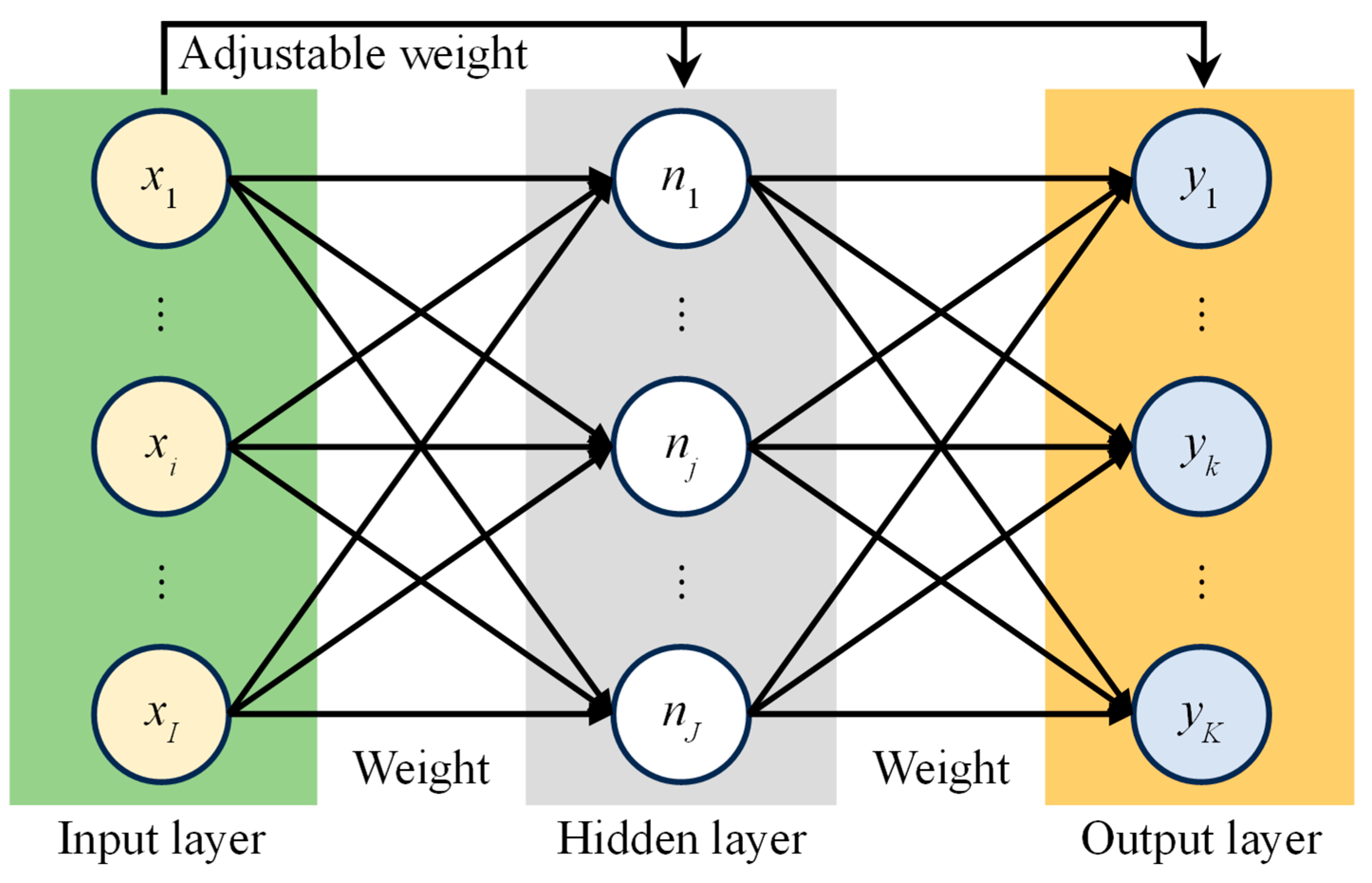
4.3.1. Cascade-Forward Neural Network

The CFNN shares structural similarities with conventional feedforward networks, as shown in Figure 7 [30]. The CFNN shares architectural similarities with feedforward networks employing backpropagation, adopting gradient-based parameter optimization through error backpropagation. This network’s distinctive architectural paradigm, however, emerges from its topological configuration, in which hidden layers maintain cross-tier linkages through progressive connectivity pathways [31]. Within the CFNN architecture, as with other feedforward networks, one or more hidden layers exist with mutual connections and nonlinear activation functions. Neurons possess individual biases, while interconnections carry specified weights. The calibration of artificial neural networks necessitates optimization of synaptic connection strengths to achieve prediction accuracy within predefined tolerance thresholds, as documented in reference [32].

The network architecture comprises three principal components: output neurons y_k (k = 1, 2, …, K), input units x_i (i = 1, 2, …, I), and hidden layer nodes n_j (j = 1, 2, …, J). While exhibiting structural parallels with conventional feedforward backpropagation architectures in employing error backpropagation for synaptic weight adjustments, the CFNN’s key differentiator resides in implementing full cross-layer connectivity, in which each neuronal layer maintains direct synaptic linkages with all antecedent processing stages [33]. The hidden layer employs the tansig nonlinear operator as its core computational transformation mechanism.

$$f(x)={\displaystyle \frac{2}{1+e^{-2x}}}-1$$

(27)

The output layer implements the purelin linear transfer operator as its transformation mechanism.

$$f(x)=x$$

(28)

4.3.2. Training of the CFNN Prediction Model of Worktable’s Dynamic Error

To train the CFNN, the Levenberg–Marquardt (LM) algorithm is utilized, which effectively integrates the optimization capabilities of the Gauss–Newton technique with the swift convergence characteristic of gradient descent [34]. The BPNN’s learning process can be essentially viewed as the solution to Equation (29).

$$\underset{S\in R^n}{\min }F(S)={\displaystyle \frac{1}{2}}{\left(r\left(S\right)\right)}^{T}r\left(S\right)={\displaystyle \frac{1}{2}}{\displaystyle \sum _{i=1}^m{\left[r_i(S)\right]}^2}\left(m\ge n\right)$$

(29)

where n denotes the sample dimension, m represents the sample’s number, and i indicates the i-th sample. r(S) is the residual function of S.

$$r\left(S\right)={\left[r_1\left(S\right),r_2\left(S\right),\dots ,r_m\left(S\right)\right]}^T$$

(30)

The matrix S is obtained by combining the weights and the bias vector.

$$S=\left[\begin{array}{ccccc}{p}_{11}& p_{12}& \dots & p_{1n}& q_1\\ p_{21}& p_{22}& \dots & p_{2n}& q_2\\ ⋮& ⋮& \ddots & ⋮& ⋮\\ p_{n1}& p_{n2}& \dots & p_{nn}& q_n\end{array}\right]$$

(31)

where p denotes the weights, and q represents the bias. The Jacobian matrix of r(S) is J_a(S).

$$J_a\left(S\right)={\left[\nabla r_1\left(S\right),\nabla r_2\left(S\right),\dots ,\nabla r_m\left(S\right)\right]}^T={\left[\begin{array}{cccc}{\displaystyle \frac{\partial r_1}{\partial S_1}}& {\displaystyle \frac{\partial r_1}{\partial S_2}}& \dots & {\displaystyle \frac{\partial r_1}{\partial S_n}}\\ {\displaystyle \frac{\partial r_2}{\partial S_1}}& {\displaystyle \frac{\partial r_2}{\partial S_2}}& \dots & {\displaystyle \frac{\partial r_2}{\partial S_n}}\\ ⋮& ⋮& \ddots & ⋮\\ {\displaystyle \frac{\partial r_m}{\partial S_1}}& {\displaystyle \frac{\partial r_m}{\partial S_2}}& \dots & {\displaystyle \frac{\partial r_m}{\partial S_n}}\end{array}\right]}^T$$

(32)

G(S) is the gradient of F(S).

$$G\left(S\right)={\displaystyle \sum _{i=1}^m{r}_i(S)\nabla r_i(S)}={\left(Ja\left(S\right)\right)}^{T}r\left(S\right)$$

(33)

At the k-th optimization stage, the gradient can be expressed mathematically as

$${\Delta }_k=-\left[{\left(J_a\left(S_K\right)\right)}^T{J}_a\left(S_K\right)+u_{k}I\right]{\left(J_a\left(S_K\right)\right)}^{T}r\left(S_K\right)$$

(34)

where I denotes the identity matrix and u_k is the step size parameter. A larger u_k causes the Levenberg–Marquardt (LM) algorithm to approximate gradient descent, as the diagonal terms dominate the update. In contrast, a smaller u_k shifts the LM method toward the Gauss–Newton approach [35]. During the training of the prediction model, performance assessment is essential. For this purpose, the absolute error (AE) metric is employed to evaluate the model’s accuracy.

$$A{E}_i=\left|{\widehat{y}}_i-y_i\right|$$

(35)

where ${\widehat{y}}_i$ represents the output of the CFNN for the i-th sample point, and y_i denotes the output of the i-th sample. When training the CFNN, the number of neurons M_h in the h-th hidden layer, the number of hidden layers N, the number of iterations epochs, and the learning rate u influence the performance of the CFNN. A total of 1000 samples were randomly generated using LHS and the electromechanical coupling model to evaluate the performance of the CFNN.

Table 7. Maximum and average AE of worktable position for different u.

	u = 0.3	u = 0.5	u = 0.7
Maximum AE (mm)	118.9	40.39	25.62
Average AE (mm)	15.08	5.559	2.622

shows the worktable position’s maximum and average absolute errors when the learning rate u is set to 0.3, 0.5, and 0.7, respectively (N = 1, M₁ = 3, epochs = 100).

Table 8. Maximum and average AE of worktable position for different N.

	N = 1	N = 2	N = 3
Maximum AE (mm)	118.9	26.62	15.23
Average AE (mm)	15.08	1.674	0.631

presents the worktable position’s maximum and mean absolute errors when the number of hidden layers N is set to 1, 2, and 3, respectively (M₁ = M₂ = M₃ = 3, epochs = 100, u = 0.3).

Table 9. Maximum and average AE of worktable position for different M_h.

	Mh = 3	Mh = 4	Mh = 5
Maximum AE (mm)	15.23	8.558	5.545
Average AE (mm)	0.631	0.309	0.112

displays the workbench position’s maximum and mean absolute errors when the number of neurons M_h in the hidden layer is set to 3, 4, and 5, respectively (N = 3, epochs = 100, u = 0.3).

Table 10. Maximum and average AE of worktable position for different epochs.

	epochs = 100	epochs = 150	epochs = 200
Maximum AE(μm)	15.2320	10.7695	7.0424
Average AE (mm)	0.6314	0.4880	0.3277

illustrates the workbench position’s maximum and mean absolute errors when the number of iterations epochs is set to 100, 150, and 200, respectively (N = 3, M₁ = M₂ = M₃ = 3, u = 0.3). Table 7, Table 8, Table 9 and Table 10 demonstrate that the accuracy of the CFNN improves as N, M_h, and epochs increase and as u decreases. It is worth noting that excessively large or small values of N, M_h, u, and epochs may lead to overfitting or underfitting of the CFNN, resulting in degraded performance.

The steps for constructing a neural network are summarized in reference [36]. The final parameters are N = 3, M₁ = 34 M₂ = 19, M₃ = 8, u = 0.97, and epochs = 500. A CFNN with an input layer consisting of four nodes and an output layer with one node was trained. The inputs to the CFNN are S_w(k), ${\dot{S}}_{w\left(k\right)}$, ${\ddot{S}}_{w\left(k\right)}$, and I_qr(k), while the output is ${\widehat{S}}_{w(k+1)}$. The input range for S_w(k) is 0 to 1500 mm, for ${\dot{S}}_{w\left(k\right)}$ it is −333 to 333 mm/s, for ${\ddot{S}}_{w\left(k\right)}$ it is −1000 to 1000 mm/s², and for I_qr(k) it is −15 to 15 A.

4.3.3. Validation and Testing of CFNN

An additional 1000 random sample points were generated using LHS and the electromechanical coupling model to test and validate the CFNN. The validation samples were input into the electromechanical coupling model and the CFNN, and the results from the electromechanical coupling model and the CFNN were obtained, respectively.

Table 11. Maximum and average AE of the trained CFNN.

Maximum AE (μm)	Average AE (μm)
9.549 × 10−9	2.572 × 10−9

presents the maximum and mean absolute errors of the trained CFNN. The CFNN model demonstrates sufficient accuracy in predicting ${\widehat{S}}_{w(k+1)}$. The predicted tracking error of the worktable, ${\widehat{E}}_{w(k+1)}$, can be predicted by subtracting the predicted worktable position ${\widehat{S}}_{w(k+1)}$ from the reference position S_wr(k+1) at time k, as shown in Equation (36).

$${\widehat{E}}_{w\left(k+1\right)}=S_{wr(k+1)}-{\widehat{S}}_{w\left(k+1\right)}$$

(36)

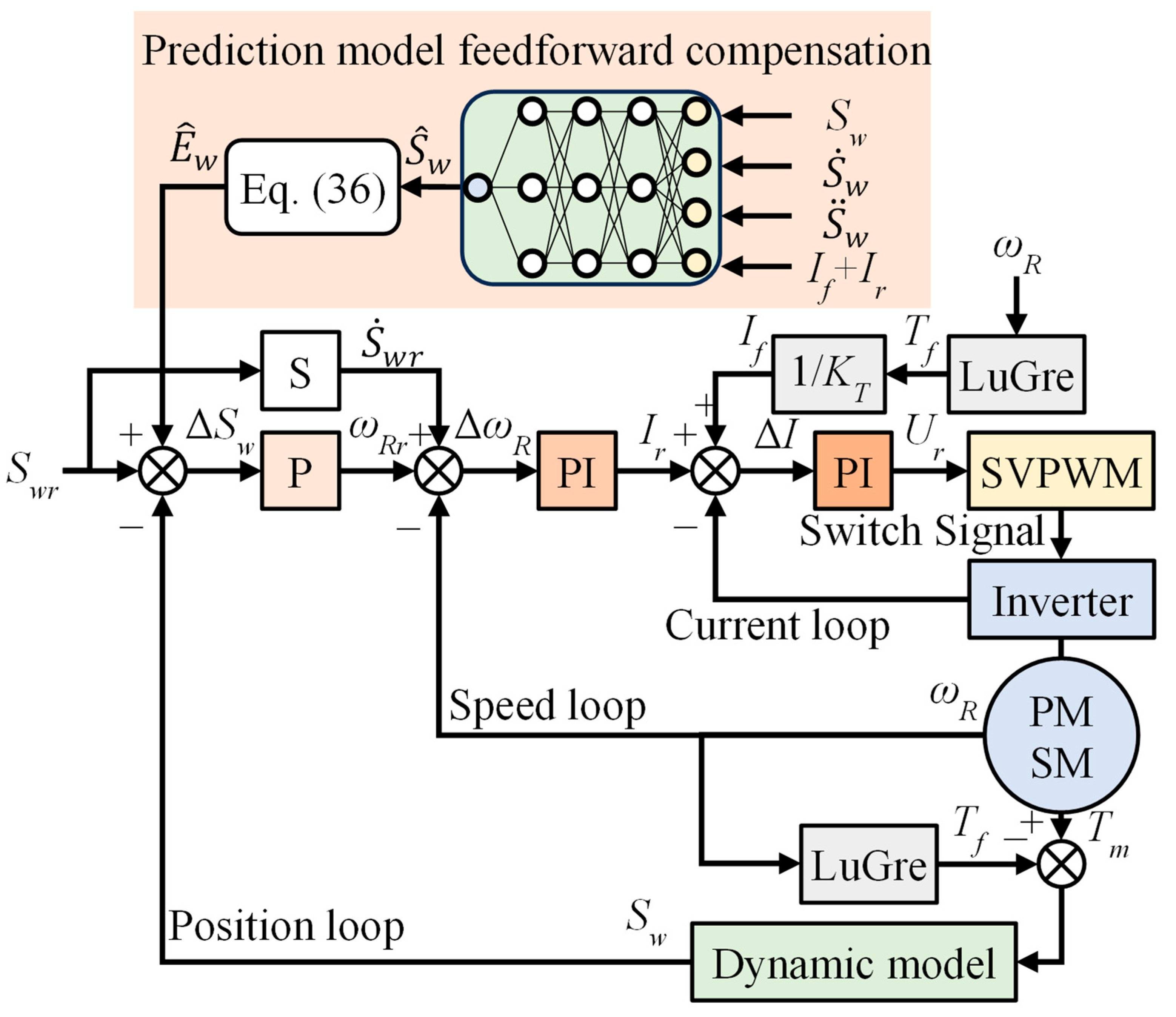
4.4. Feedforward Compensation Structure Based on the Prediction Model

The feedforward compensation structure is illustrated in Figure 8. Firstly, the prediction model is employed to calculate ${\widehat{S}}_w$. Subsequently, the predicted tracking error ${\widehat{E}}_w$ is obtained using Equation (36). Finally, the tracking error ${\widehat{E}}_w$ is applied to the position loop. When the feedforward compensation is incorporated, the input to the position loop P controller becomes ΔS_w = S_wr − S_w + ${\widehat{E}}_w$. The remaining control structure remains consistent with that depicted in Figure 5. The Lugre model was also used to compensate for friction, where K_T represents the torque constant.

5. Simulation and Experiment

In this section, simulations and experiments using typical trajectories validate the effectiveness of the electromechanical coupling model, the dynamic error prediction model, and the feedforward compensation strategy. The electromechanical coupling model is compared with the experimental results. The dynamic error prediction model is compared with the transfer function approach [37]. A sampling rate of 10 kHz is used for all the simulations and experiments.

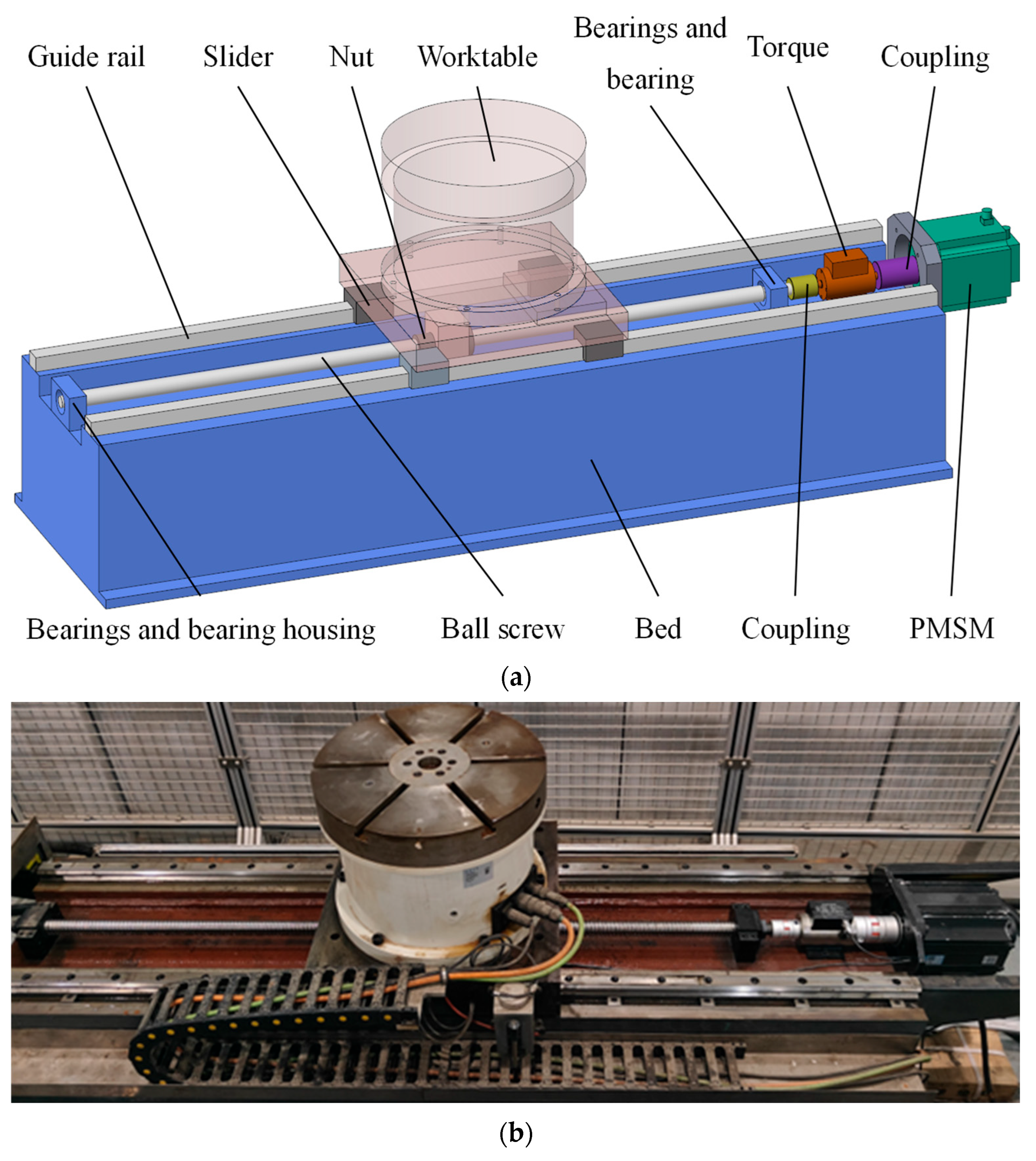
5.1. Ball Screw Feed System Experimental Test Platform

Figure 9 illustrates the experimental setup of the ball screw feed system. The setup comprises a HEIDENHAIN LC185ML1840 grating scale, a worktable equipped with a rotary stage, two BK30 bearing blocks with two bearings, two HIWIN HGH45CA linear guides with four sliders, a HIWIN FDI40-10T3 ball screw with a nut, a HAIBOHUA HCNJ-101 dynamic torque sensor, two MJC-65-BL couplings, a machine bed, and a Hilectro PMSM. An encoder is mounted on the PMSM to provide feedback on the angular position and velocity of the PMSM rotor. The grating scale measures the position of the worktable. The current signals of the PMSM are acquired by the PMSM driver DY2H. The OP4510v2 collects feedback signals from the grating scale, the PMSM encoder, and the motor driver DY2H. Based on these feedback signals, the OP4510v2 generates control signals for the PMSM in each control cycle, which are then transmitted through the DY2H to drive the PMSM. A computer is employed to control the OP4510v2. Simulation and experimental programs are developed and compiled on the PC using RT-LAB software and downloaded to the OP4510v2 for execution.

5.2. Simulation and Experimentation of Typical Trajectories

Six S-shaped velocity interpolation trajectories were designed to validate the compensation effectiveness, each characterized by distinct velocity, acceleration, and jerk profiles.

Table 12. The parameters of the six S-curve velocity interpolation trajectories.

Trajectories	Displacement	Maximum Velocity	Maximum Acceleration	Maximum Jerk
1	300	100	225	1200
2	300	100	225	1400
3	300	100	120	1000
4	300	100	140	1000
5	300	110	160	1000
6	300	120	160	1000

enumerates the parameters of these six S-shaped velocity interpolation trajectories.

The distinction between Trajectory 1 and Trajectory 2 lies in their jerk values, while Trajectory 3 and Trajectory 4 differ in acceleration, and Trajectory 5 and Trajectory 6 vary in velocity. Figure 10 graphically presents these six S-shaped velocity interpolation trajectories.

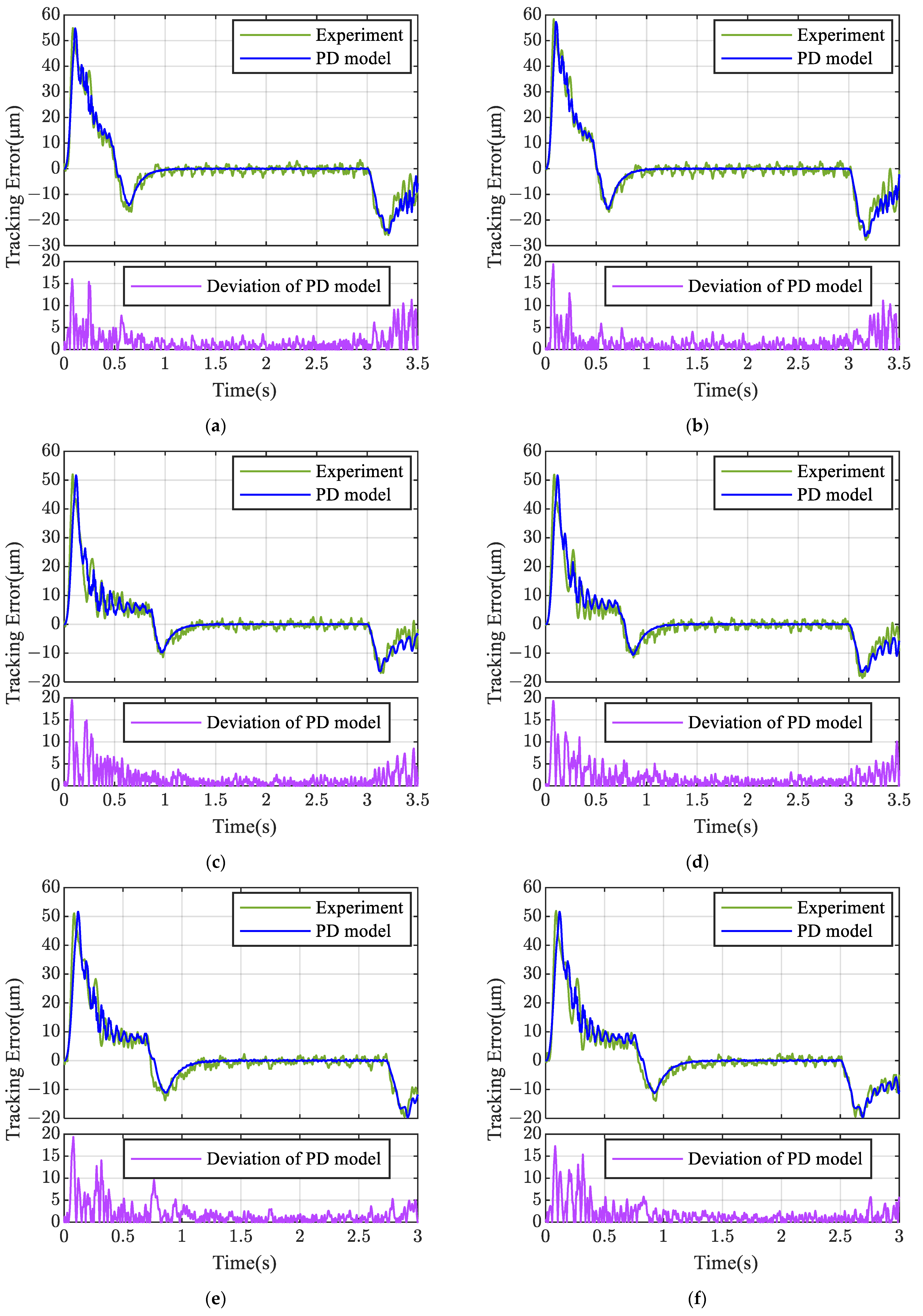
5.2.1. Electromechanical Coupling Model Simulation and Experimentation

Figure 11 presents the tracking errors obtained from simulations based on the electromechanical coupling model under the six trajectories alongside the experimentally measured tracking errors from the ball screw feed system test platform. In Figure 11, the green line represents the experimental results, the blue line corresponds to the position-dependent electromechanical coupling model, and the purple line indicates the deviations of the position-dependent (PD) model.

Table 13. Maximum/average tracking errors of electromechanical coupling simulation and experiment.

Trajectories	Experiment		Position-Dependent
	Maximum Tracking Error (μm)	Average Tracking Error (μm)	Maximum Tracking Error (μm)	Average Tracking Error (μm)
1	54.86	6.753	54.75	5.757
2	58.35	7.013	57.3	5.848
3	51.98	5.056	51.64	4.482
4	51.89	5.279	51.64	4.771
5	51.08	6.38	51.64	5.552
6	51.91	6.719	51.64	6.052

lists the corresponding maximum tracking errors and average tracking errors.

As shown in Figure 11 and Table 13, the maximum and average tracking errors of the position-dependent electromechanical coupling model are closer to the experimental results. The maximum acceleration of Trajectory 2 resulted in the most significant tracking error. Regardless of variations in velocity or acceleration, their impact on the tracking error of the ball screw feed system is relatively minor. In contrast, the influence of jerk on tracking error is more pronounced.

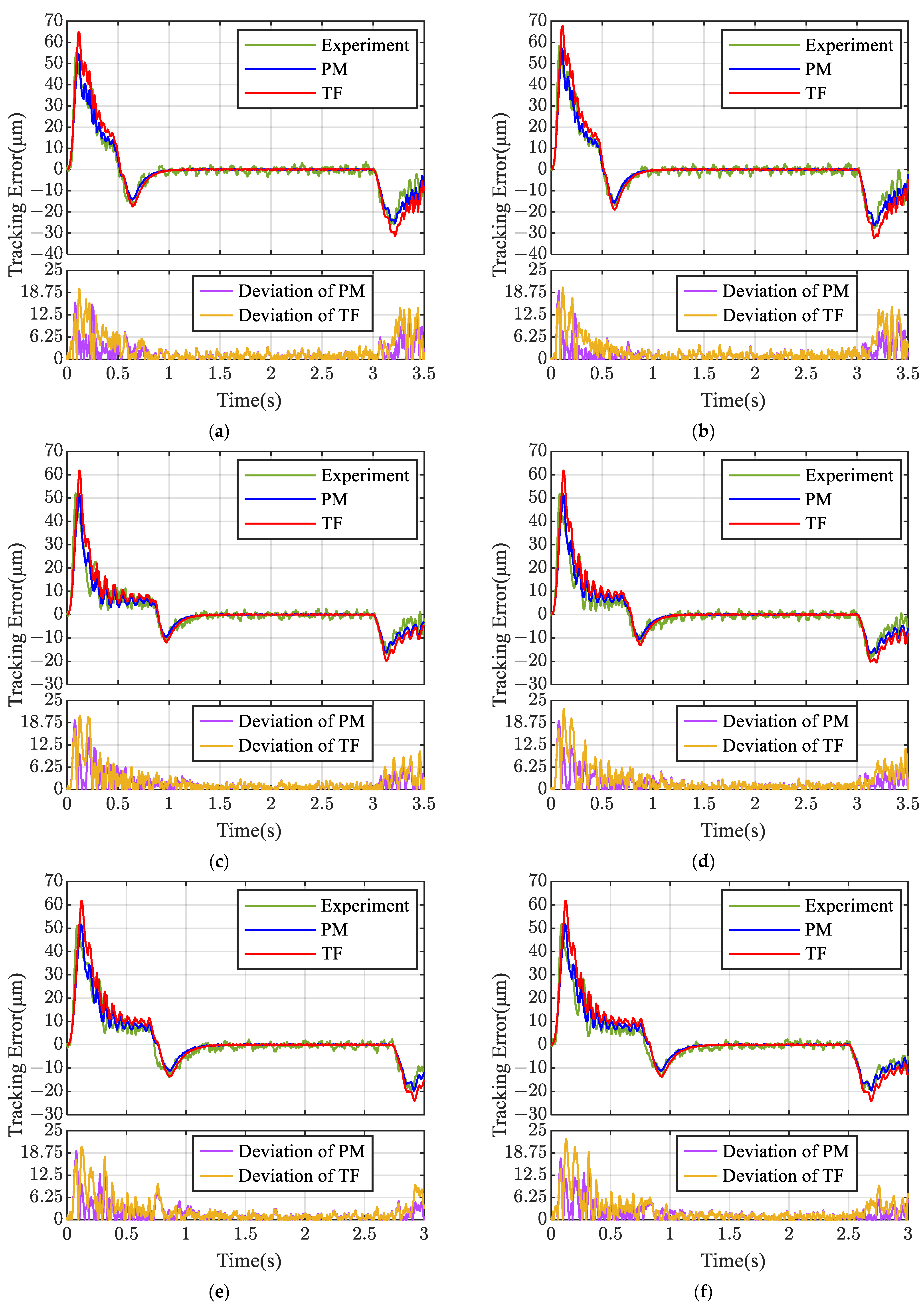
5.2.2. Dynamic Error Prediction

Figure 12 illustrates the tracking errors obtained from simulations based on the prediction model and transfer function under the six trajectories alongside the experimentally measured tracking errors from the ball screw feed system test platform. In Figure 12, the green line represents the experimental results; the blue line corresponds to the prediction model (PM); the red line represents the transfer function (TF); the purple line indicates the deviations of the SM; and the orange line denotes the deviations of the TF.

Table 14. Maximum/average tracking error prediction simulation and experiment.

Trajectories	Experiment		Prediction Model		Transfer Function
	Maximum Tracking Error (μm)	Average Tracking Error (μm)	Maximum Tracking Error (μm)	Average Tracking Error (μm)	Maximum Tracking Error (μm)	Average Tracking Error (μm)
1	54.86	6.804	54.75	6.574	64.75	7.573
2	58.35	7.098	57.3	6.173	67.75	7.694
3	51.98	5.056	51.64	4.709	61.79	5.878
4	51.89	5.279	51.64	5.098	61.79	6.261
5	51.08	6.414	51.64	5.862	61.79	7.313
6	51.91	6.719	51.64	6.407	61.79	7.995

lists the corresponding maximum tracking errors and average tracking errors.

Figure 12 and Table 14 indicate that the prediction model exhibits a maximum prediction deviation of 1.8% for the maximum tracking error and 13% for the average tracking error. In contrast, the transfer function demonstrates a maximum prediction deviation of 21% for the maximum and 19% for the average tracking error. These comparisons indicate that the prediction model provides significantly higher accuracy in predicting tracking errors.

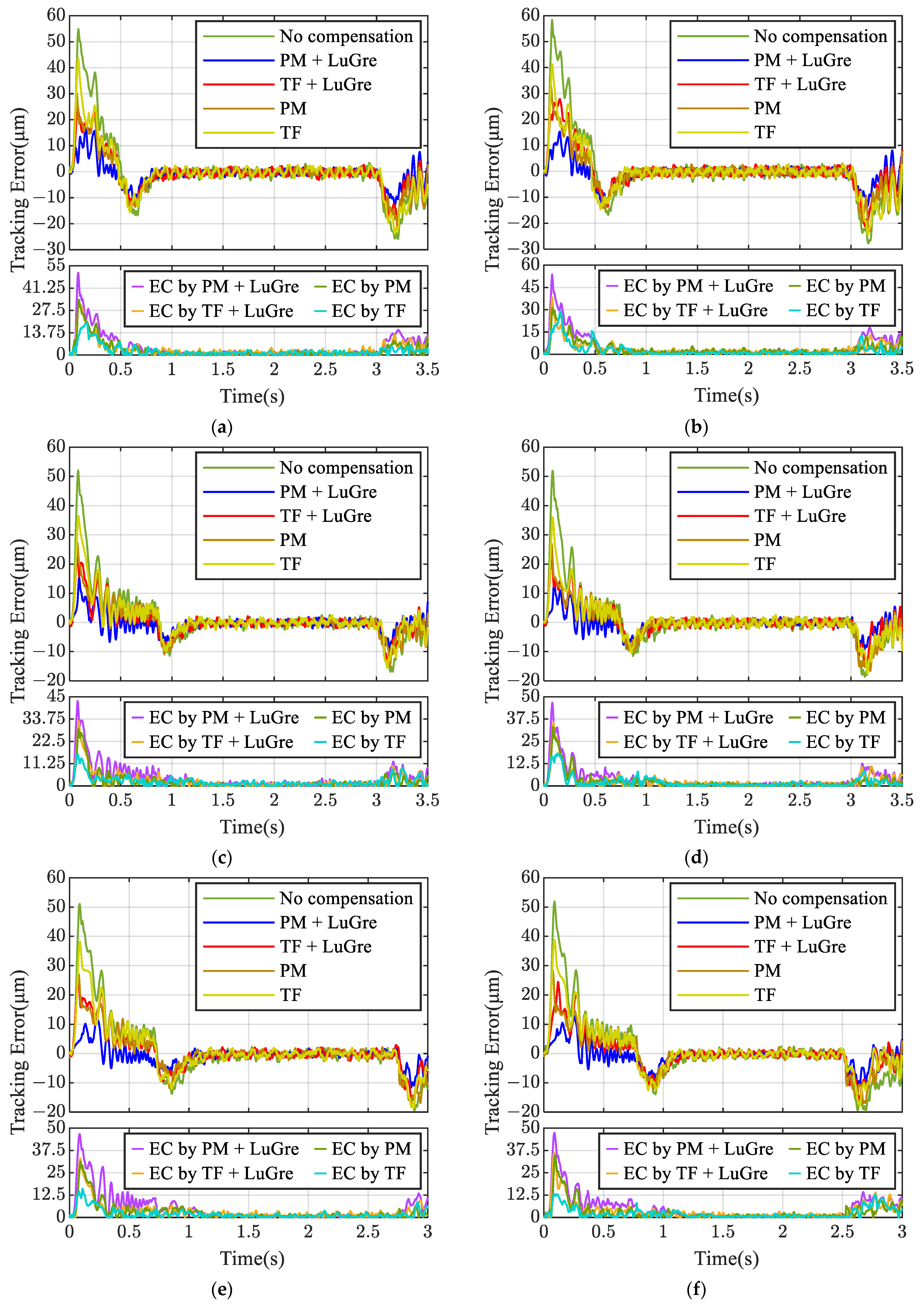
5.2.3. Dynamic Error Compensation

Figure 13 presents the experimental tracking errors for the six trajectories under five conditions: without compensation, the proposed PM feedforward compensation method with LuGre friction compensation, and transfer function feedforward compensation with LuGre friction compensation, the proposed PM feedforward compensation method without LuGre friction compensation, and transfer function feedforward compensation without LuGre friction compensation. In Figure 13, the green line represents the experimental results without compensation; the blue line corresponds to the proposed feedforward compensation method and LuGre friction compensation; the red line represents the transfer function feedforward compensation method and LuGre friction compensation; the brown line represents the proposed feedforward compensation method without LuGre friction compensation; the faint yellow line corresponds to the transfer function feedforward compensation method without LuGre friction compensation; the purple line indicates the errors compensated (EC) after applying the proposed compensation method and LuGre friction compensation; the orange line denotes the errors compensated after applying the transfer function feedforward compensation and LuGre friction compensation; the dark green line indicates the errors compensated after applying the proposed compensation method without LuGre friction compensation; and the indigo line denotes the errors compensated after applying the transfer function feedforward compensation without LuGre friction compensation.

Table 15. Maximum/average tracking error for tracking error compensation experiment.

Trajectories	No Compensation		PM+ LuGre		TF+ LuGre
	Maximum Tracking Error (μm)	Average Tracking Error (μm)	Maximum Tracking Error (μm)	Average Tracking Error (μm)	Maximum Tracking Error (μm)	Average Tracking Error (μm)
1	54.86	6.804	17.07	2.705	25.21	4.33
2	58.35	7.098	15.32	2.781	27.92	4.63
3	51.98	5.056	17.19	2.275	23.39	3.28
4	51.89	5.279	19.07	2.331	22.35	3.22
5	51.08	6.414	11.88	2.317	25.3	4.076
6	51.91	6.719	12.79	2.512	24.52	4.032

lists the corresponding maximum tracking errors and average tracking errors;

Table 16. Maximum/average tracking error for the tracking error compensation experiment without friction compensation.

Trajectories	PM		TF
	Maximum Tracking Error (μm)	Average Tracking Error (μm)	Maximum Tracking Error (μm)	Average Tracking Error (μm)
1	30.09	4.443	43.67	5.177
2	33.21	4.404	41.22	5.183
3	27.39	3.337	36.50	3.666
4	27.16	3.432	36.01	3.872
5	27.10	4.152	38.20	4.860
6	28.59	4.340	38.84	4.912

lists the corresponding maximum tracking errors and average tracking errors without LuGre friction compensation.

Figure 13 and Table 15 demonstrate that the proposed method with LuGre friction compensation achieves a maximum reduction rate of 76.7% for the maximum tracking error and 63.7% for the average tracking error. The transfer function feedforward compensation method with LuGre friction compensation attains a maximum reduction rate of 56.9% for the maximum and 40% for the average tracking error. These comparisons indicate that the proposed compensation method is more effective in reducing tracking errors. As can be seen from Figure 13, Table 15 and Table 16, the friction compensation further reduces the maximum and average tracking errors for the proposed method and the transfer function. Specifically, the maximum tracking error of the proposed method is reduced by 56.1% and the average tracking error by 44.1%, while the transfer function demonstrates a 42.2% reduction in maximum tracking error and a 17.9% decrease in average tracking error.

6. Conclusions

This paper presents a prediction-model-based approach for predicting and compensating dynamic errors in ball screw feed systems. Initially, the lumped mass method and distributed mass method were employed to establish a dynamic model of the ball screw feed system relying on the moving components’ positions, which is then extended to construct an electromechanical coupling model. LHS and the electromechanical coupling model were utilized to generate sample points for training a CFNN prediction model to predict the worktable position and dynamic errors within a control cycle. The simulation and experimental results demonstrate the dynamic error prediction model’s deviations of 1.8% for the maximum tracking error and 13% for the average tracking error, outperforming the transfer function method’s 21% and 19%, respectively. The simulation and experimental results demonstrate the high accuracy of the proposed position-dependent electromechanical coupling model and the dynamic error prediction model. Subsequently, a compensation strategy was proposed. The experimental results indicate that the proposed compensation method with friction compensation achieves maximum reduction rates of 76.7% for the maximum tracking error and 63.7% for the average tracking error, which are better than the transfer function compensation with friction compensation’s 56.9% and 40%, respectively. Comparisons with the transfer function feedforward compensation experiments and uncompensated experiments confirmed the effectiveness of the proposed compensation method.

Future work includes applying transfer learning to the prediction model using experimental data to enhance the accuracy further; extending the prediction model to multi-axis feed systems; and accounting for the thermal error by simultaneously compensating for both thermal and dynamic errors, thereby improving tracking precision.

References

1. Liu, X.; Li, Y.G.; Cheng, Y.G.; Cai, Y. Sparse identification for ball-screw drives considering position-dependent dynamics and nonlinear friction. Robot. Comput.-Integr. Manuf. 2023, 81, 102486. [Google Scholar] [CrossRef]
2. Zhu, M.; Bao, D.; Huang, X. The Design of a Tracking Controller for Flexible Ball Screw Feed System Based on Integral Sliding Mode Control with a Generalized Extended State Observer. Robot. Actuators 2023, 12, 387. [Google Scholar] [CrossRef]
3. Zhang, L.; Liu, J.H.; Zhuang, C.B.; Yao, M.Q.; Chen, F.H.; Zhang, C.Y. Gain scheduling control of ball screw feed drives based on linear parameter varying model. Int. J. Adv. Manuf. Technol. 2023, 124, 4493–4510. [Google Scholar] [CrossRef]
4. Liu, Z.D.; Li, C.Y.; Wang, G.D.; Yang, X.D.; Xu, M.T.; Li, Z.Y.; Li, J.J. Modeling and investigation on dynamic behaviors of ball screw feed system with bolt looseness. Int. J. Nonlinear Mech. 2025, 170, 104996. [Google Scholar] [CrossRef]
5. Gong, X.X.; Zhao, J.S.; Zhao, C.Y.; Li, C.Y.; Hao, J.; Xu, M.T. Dynamic modeling and nonlinear characteristic analysis of the cross-axis ball screw feed system considering thermal deformation. Nonlinear Dyn. 2025, 113, 14515–14560. [Google Scholar] [CrossRef]
6. Zhang, H.J.; Zhang, J.; Liu, H.; Liang, T.; Zhao, W.H. Dynamic modeling and analysis of the high-speed ball screw feed system. Proc. Inst. Mech. Eng. Part B-J. Eng. Manuf. 2014, 229, 870–877. [Google Scholar] [CrossRef]
7. Vicente, D.A.; Hecker, R.L.; Villegas, F.J.; Flores, G.M. Modeling and vibration mode analysis of a ball screw drive. Int. J. Adv. Manuf. Technol. 2012, 58, 257–265. [Google Scholar] [CrossRef]
8. Lu, H.J.; Rui, X.T.; Ma, Z.Y.; Ding, Y.Y.; Chen, Y.H.; Chang, Y.; Zhang, Y.P. Hybrid multibody system method for the dynamic analysis of an ultra-precision fly-cutting machine tool. Int. J. Mech. Syst. Dyn. 2022, 2, 290–307. [Google Scholar] [CrossRef]
9. Miao, H.H.; Wang, C.Y.; Hao, J.; Li, C.Y.; Xu, M.T.; Liu, Z.D. Dynamic analysis of the column-spindle system considering the nonlinear characteristics of kinematic joints. Mech. Mach. Theory 2022, 174, 104922. [Google Scholar] [CrossRef]
10. Hu, Y.J.; Wang, Y.Y.; Zhu, W.D.; Li, H.L. Dynamic Modeling of a Ball-Screw Drive and Identification of Its Installation Parameters. J. Dyn. Syst. Meas. Control-Trans. ASME 2021, 143, 041003. [Google Scholar] [CrossRef]
11. He, W.W.; Wang, L.P.; Guan, L.W. A novel approach to calculating the dynamic error reflected on an S-shaped test piece. Proc. Inst. Mech. Eng. Part C-J. Eng. Mech. Eng. Sci. 2021, 235, 3273–3298. [Google Scholar] [CrossRef]
12. Lyu, D.; Liu, Q.; Luo, S.Y.; Wang, D.W.; Liu, H. The influence of dynamic error outside servo-loop on the trajectory error. Int. J. Adv. Manuf. Technol. 2021, 113, 1517–1525. [Google Scholar] [CrossRef]
13. Yang, L.; Zhang, X.; Wang, L.; Zhao, W.H. Dynamic error of multi-axis machine tools considering position dependent structural dynamics and axis coupling inertial forces. Proc. Inst. Mech. Eng. Part B-J. Eng. Manuf. 2022, 236, 281–295. [Google Scholar] [CrossRef]
14. Hu, J.J.; Yang, D.Z.; Sun, Z.C. Torque Fluctuation Suppression Strategy of Integrated Electric Drive System Based on the Principle of Minimization of Instantaneous Current Tracking Error. IEEE Access 2022, 10, 124673–124684. [Google Scholar] [CrossRef]
15. Jiang, J.L.; LI, B.R.; Lin, F.Y.; Zhang, H.; Ye, P.Q. Prediction and compensation strategy of contour error in multi-axis motion system. Int. J. Adv. Manuf. Technol. 2022, 119, 163–175. [Google Scholar] [CrossRef]
16. Zhang, J.; Li, B.; Zhou, C.X.; Zhao, W.H. Positioning error prediction and compensation of ball screw feed drive system with different mounting conditions. Proc. Inst. Mech. Eng. Part B-J. Eng. Manuf. 2016, 230, 2307–2311. [Google Scholar] [CrossRef]
17. Liu, Q.; Lu, H.; Yonezawa, H.; Yonezawa, A.; Kajiwara, I.; Jiang, T.; He, J.J. Geometric and dynamic error compensation of dual-drive machine tool based on mechanism-data hybrid method. Mech. Syst. Signal Proc. 2025, 224, 112041. [Google Scholar] [CrossRef]
18. Liu, C.; Zhao, C.Y.; Wen, B.C. Dynamics analysis on the MDOF model of ball screw feed system considering the assembly error of guide rails. Mech. Syst. Signal Proc. 2022, 178, 109290. [Google Scholar] [CrossRef]
19. Li, X.W.; Zhang, J.; Zhao, W.H.; Lu, B.H. A zero phase error tracking based path precompensation method for high-speed machining. Proc. Inst. Mech. Eng. Part C-J. Eng. Mech. Eng. Sci. 2016, 230, 230–239. [Google Scholar] [CrossRef]
20. Zhang, D.L.; Chen, H.C. A data-driven iterative pre-compensation method of contouring error for five-axis machine tools. Int. J. Adv. Manuf. Technol. 2024, 135, 1669–1684. [Google Scholar] [CrossRef]
21. Wu, H.; Meng, Y.X.; Zhao, Z.Y.; Zhu, Z.W.; Ren, M.J.; Zhang, X.Q.; Zhu, L.M. Surrogate model-based tool trajectory modification for ultra-precision tool servo diamond turning. Precis. Eng.-J. Int. Soc. Precis. Eng. Nanotechnol. 2025, 93, 46–57. [Google Scholar] [CrossRef]
22. Li, H.C.; Li, Y.F.; Huang, S.M. Optimization strategy for the control of permanent magnet synchronous motors in numerical control machine tools based on intelligent feedforward self-learning. Rev. Adhes. Adhes. 2023, 11, 744–757. [Google Scholar] [CrossRef]
23. Wang, Z.G.; Feng, X.Y.; Yang, H.T.; Jin, H.W. Research on low-speed characteristics of differential double-drive feed system. Mech. Sci. 2021, 12, 791–802. [Google Scholar] [CrossRef]
24. Jin, L.; Li, C.H.; Wang, X.; Xie, L.M. A dynamic stiffness model for high-speed ball screw pair with the mass center of screw nut considered. Mech. Ind. 2023, 24, 21. [Google Scholar] [CrossRef]
25. Li, F.; Jiang, Y.; Li, T.; Ehmann, K.F. Compensation of dynamic mechanical tracking errors in ball screw drives. Mechatronics 2018, 55, 27–37. [Google Scholar] [CrossRef]
26. Li, X.T.; Xi, D.L.; Zhang, Y.L. Permanent magnet synchronous motor vector control based on MATLAB/Simulink. In Proceedings of the 2017 First International Conference on Electronics Instrumentation & Information Systems (EIIS), Harbin, China, 3–5 June 2017. [Google Scholar] [CrossRef]
27. Lascu, C.; Trzynadlowski, A.M. A sensorless hybrid DTC drive for high-volume low-cost applications. IEEE Trans. Ind. Electron. 2004, 51, 1048–1055. [Google Scholar] [CrossRef]
28. Preitl, S.; Precup, R.E. On the algorithmic design of a class of control systems based on providing the symmetry of open-loop Bode plots. Sci. Bull. UPT 1996, 41, 47–55. [Google Scholar]
29. Meng, D.B.; Li, Y.; He, C.; Guo, J.B.; Lv, Z.Y.; Wu, P. Multidisciplinary design for structural integrity using a collaborative optimization method based on adaptive surrogate modelling. Mater. Des. 2021, 206, 109789. [Google Scholar] [CrossRef]
30. Jesús, O.D.; Hagan, M.T. Backpropagation algorithms for a broad class of dynamic networks. IEEE Trans. Neural Netw. 2007, 18, 14–27. [Google Scholar] [CrossRef]
31. Shohda, A.M.A.; Ali, M.A.M.; Ren, G.F.; Kim, J.G.; Mohamed, M.A. Application of Cascade Forward Backpropagation Neural Networks for Selecting Mining Methods. Sustainability 2022, 14, 635. [Google Scholar] [CrossRef]
32. Nami, F.; Deyhimi, F. Prediction of activity coefficients at infinite dilution for organic solutes in ionic liquids by artificial neural network. J. Chem. Thermodyn. 2011, 43, 22–27. [Google Scholar] [CrossRef]
33. Yavuz, M.; Iphar, M.; Once, G. The optimum support design selection by using AHP method for the main haulage road in WLC Tuncbilek colliery. Tunn. Undergr. Space Technol. 2008, 23, 111–119. [Google Scholar] [CrossRef]
34. Zhang, J.S.; Tian, J.L.; Alcaide, A.M.; Leon, J.I.; Vazquez, S.; Franquelo, L.G.; Luo, H.; Yin, S. Lifetime extension approach based on the Levenberg–Marquardt neural network and power routing of DC-DC converters. IEEE Trans. Power Electron. 2023, 38, 10280–10291. [Google Scholar] [CrossRef]
35. Wang, S.W.; Yuan, Y.; Zhou, A.H.; Yin, C. Environmental Study on Analysis of Characteristic Parameters of Rockfall Movement Based on Field Riprap Test and Establishment of SVM and LM-BPNN Prediction Models. Ekoloji Dergisi 2019, 28, 3319–3326. [Google Scholar]
36. Dong, P.; Li, J.Q.; Guo, W.; Lai, J.B.; Mao, F.H.; Wang, K.F.; Xu, X.Y.; Wang, S.H. Surrogate-assisted multi-objective optimization for control parameters of adjacent gearshift process with multiple clutches. Control Eng. Practice. 2023, 135, 105519. [Google Scholar] [CrossRef]
37. Cui, Y.X.; Zhong, B.; Qian, W.K.; Zheng, C.J. Identification of Time Series Transfer Function Parmeter. In Proceedings of the 2014 International Conference on Mechatronics Electronic industrial and Control Engineering (MEIC 2014), Shenyang, China, 15–17 November 2014. [Google Scholar] [CrossRef]
Figure 1. Overview of dynamic error prediction and compensation methods for the ball screw feed system.
Machines 13 00433 g001
Figure 2. Ball screw feed system: (a) ball screw feed system’s configuration; (b) real ball screw feed system.
Machines 13 00433 g002
Figure 3. Two-element Timoshenko beam after length adjustment.
Machines 13 00433 g003
Figure 4. Position-dependent dynamic model of the ball screw feed system.
Machines 13 00433 g004
Figure 5. Electromechanical coupling model of the ball screw feed system.
Machines 13 00433 g005
Figure 6. The principle of predicting the position of the worktable of one control cycle.
Machines 13 00433 g006
Figure 7. The Cascade-Forward Neural Network.
Machines 13 00433 g007
Figure 8. Feedforward compensation structure.
Machines 13 00433 g008
Figure 9. The ball screw feed system experimental platform.
Machines 13 00433 g009
Figure 10. S-curve velocity interpolation trajectories: (a) Velocity; (b) acceleration; (c) jerk.
Machines 13 00433 g010
Figure 11. Electromechanical coupling simulation and experimental tracking errors: (a) Trajectory 1; (b) Trajectory 2; (c) Trajectory 3; (d) Trajectory 4; (e) Trajectory 5; (f) Trajectory 6.
Machines 13 00433 g011
Figure 12. Tracking error prediction simulation and experimental tracking error: (a) Trajectory 1; (b) Trajectory 2; (c) Trajectory 3; (d) Trajectory 4; (e) Trajectory 5; (f) Trajectory 6.
Machines 13 00433 g012
Figure 13. Tracking error compensation experiment: (a) Trajectory 1; (b) Trajectory 2; (c) Trajectory 3; (d) Trajectory 4; (e) Trajectory 5; (f) Trajectory 6.
Machines 13 00433 g013