Abstract
This research presents an advanced autonomous HVAC control system tailored for a chemical fiber factory, emphasizing the human-centric principles and collaborative potential of Industry 5.0. The system architecture employs several functional levels—actuator and sensor, process, model, critic, fault detection, and specification—to effectively monitor and predict indoor air pressure differences, which are critical for maintaining consistent product quality. Central to the system’s innovation is the integration of digital twins and physical AI, enhancing real-time monitoring and predictive capabilities. A virtual representation runs in parallel with the physical system, enabling sophisticated simulation and optimization. Development involved custom sensor kit design, embedded systems, IoT integration leveraging Node-RED for data streaming, and InfluxDB for time-series data storage. AI-driven system identification using Nonlinear Autoregressive with eXogenous inputs (NARX) neural network models significantly improved accuracy. Crucially, incorporating airflow velocity data alongside AHU output and past pressure differences boosted the NARX model’s predictive performance (R2 up to 0.9648 on test data). Digital twins facilitate scenario testing and optimization, while physical AI allows the system to learn from real-time data and simulations, ensuring adaptive control and continuous improvement for enhanced operational stability in complex industrial settings.
1. Introduction
In the dynamic landscape of industrial development, Industry 5.0 represents the next evolutionary step beyond Industry 4.0, emphasizing human–machine collaboration and intelligent automation [1,2]. At its core, Industry 5.0 is driven by autonomous control systems—advanced technologies that enable machines to operate independently, making informed decisions with minimal human oversight [3]. This autonomy is made possible through the integration of artificial intelligence (AI), machine learning (ML), the Internet of Things (IoT), and advanced robotics. This research highlights how incorporating heating, ventilation, and air conditioning (HVAC) systems within this framework exemplifies the comprehensive and interconnected nature of Industry 5.0, enhancing efficiency, adaptability, and precision in industrial environments.
Industry 5.0, known as the “human-centered industrial revolution”, extends the advancements of Industry 4.0 by prioritizing collaboration between humans and machines [4]. Unlike its predecessor, which focused on full automation and digitalization, Industry 5.0 integrates artificial intelligence (AI), robotics, the Internet of Things (IoT), and advanced analytics to enhance human capabilities rather than replace them. This approach promotes a more sustainable, efficient, and ethical industrial environment where humans and machines work together to optimize productivity, innovation, and flexibility in manufacturing.
Heating, ventilation, and air conditioning (HVAC) systems play a crucial role in industrial settings by regulating temperature, humidity, and air quality to ensure a comfortable and safe working environment [5,6,7,8]. These systems include heating components such as furnaces, boilers, and heat pumps, ventilation mechanisms for fresh air exchange and pollutant removal, and air conditioning units that control temperature and humidity [9]. In large-scale industrial operations, maintaining optimal air pressure balance is essential to prevent issues like moisture buildup, mold growth, and air contamination, all of which can impact both worker health and equipment efficiency [10].
Air velocity and pressure differences are closely interconnected, influencing HVAC system performance and industrial operations [11,12]. Wind speed results from pressure gradients, where higher differences create stronger airflow [13]. In HVAC systems, airflow velocity is determined by factors such as duct size, fan capacity, system resistance, and static pressure [14]. Effectively managing these variables ensures precise pressure control, reduces energy consumption, and enhances overall system efficiency.
The tools available for regulating air pressure differentials within chemical plants include sensor kits utilizing microcontrollers with I2C communication, NTP synchronization, and OTA updates, alongside data collection and streaming platforms like Node-RED, data storage solutions such as InfluxDB, and visualization tools like Grafana and SVG nodes. The current stage of research, as presented, focuses on developing integrated autonomous control system architectures within the Industry 5.0 framework to predict and manage these differentials, employing AI techniques like NARX models and implementing retraining workflows based on error autocorrelation analysis to enhance prediction accuracy and maintain model fitness. The current state of development is demonstrated by the design and installation of such a sensor-based system in a chemical fiber factory, indicating that these advanced, human-centric autonomous control systems are moving towards practical implementation and validation in specific industrial environments.
In chemical fiber production, precise air pressure control is essential to maintaining consistent fiber quality and ensuring a safe working environment. During fiber extrusion, stable air pressure is required to regulate fiber diameter and structural integrity, while in cleanroom environments, controlled airflow prevents contamination and optimizes manufacturing conditions. Furthermore, proper ventilation reduces the accumulation of volatile chemicals and enhances worker safety.
This research focuses on developing an intelligent, sensor-based autonomous control system to regulate indoor air pressure differences in a chemical fiber factory. Designed within the framework of Industry 5.0, the system incorporates multiple functional layers—including actuators, sensors, process modelling, fault detection, and predictive analysis—to optimize human–machine collaboration. The system integrates IoT technology, embedded systems, and AI-driven analytics to enable real-time monitoring, data integration, and predictive maintenance. By enhancing automation while maintaining human oversight, the proposed system improves operational stability, energy efficiency, and overall productivity in industrial environments. The structure of this paper is as follows: Section 2 presents detailed background on HVAC systems, digital twins, physical AI, and human–machine decision support systems; Section 3 presents the materials and methods, including the design of the systems, performance testing, and experimental setup; Section 4 discusses the results and analysis, focusing on model prediction; and Section 5 concludes the paper with key findings.
2. Background and Related Works
The emergence of Industry 5.0 represents a pivotal shift in industrial innovation, marking a transition from automated processes to integrating advanced technology with human intelligence [15]. This goes beyond the digital and automated frameworks established by Industry 4.0, emphasizing a synergy between human expertise and innovative technology. While the early industrial revolutions replaced manual labor with steam and water-driven machinery in the 18th century, electrification and assembly lines in the 19th century introduced mass production [16,17]. The 20th century saw the rise of computer-driven automation, and now Industry 5.0 leverages artificial intelligence (AI), machine learning (ML), the Internet of Things (IoT), robotics, digital twins, and physical AI to enhance human capabilities. The focus is on sustainability, ethical manufacturing, and empowering workers.
At the heart of this new era are autonomous control systems, which enable machines to make real-time decisions with minimal human intervention [18,19]. These systems adopt a multi-layered approach, integrating sensor data, process modelling, fault detection, and predictive analytics to form robust frameworks for industrial automation [20]. Research has shown that such layered systems improve operational stability and foster human–machine collaboration, paving the way for more adaptable manufacturing environments [1,21].
Recent advancements in dynamic fault detection and predictive maintenance have made it possible to anticipate system anomalies using machine learning algorithms [22]. This allows industries to proactively adjust operational parameters, reducing downtime and improving system resilience. The integration of extensive sensor networks and IoT devices enables real-time data aggregation and analysis, making manufacturing systems more responsive and efficient, especially in complex industrial settings [23].
Additionally, advancements in embedded systems have led to the creation of flexible and scalable control platforms [24]. These platforms combine hardware and software to precisely regulate environments and adapt to fluctuating conditions. In fiber chemical manufacturing, for example, maintaining strict air pressure control is essential for product consistency and the safety of workers managing volatile chemicals.
Parallel to these technical improvements, research into human–machine collaboration stresses the importance of developing intuitive interfaces and decision-support systems [25]. These systems empower human operators to monitor, interact with, and fine-tune automated processes, striking a crucial balance between the efficiency of automation and human judgment [26]. This balance is key to optimizing production quality and fostering an environment where human expertise complements technological advancements.
The integration of digital twins and physical AI further enhances this collaboration. A digital twin is a virtual representation of a physical object, process, or system, allowing real-time monitoring, simulation, and optimization [27,28,29]. As they are continuously updated based on real-world data, digital twins provide insights into performance, potential issues, and opportunities for improvement [30,31]. In manufacturing, digital twins allow for predictive modelling, process optimization, and better decision-making, while enabling industries to evaluate different scenarios without the risks associated with physical trials.
Digital twins have gained increasing traction in the manufacturing sector due to their ability to create digital replicas of physical objects, processes, or systems. These models enable real-time data acquisition, analysis, and simulation, facilitating improvements in process optimization, predictive maintenance, and overall operational efficiency.
- Sustainable Manufacturing: A study by Kritzinger et al. (2018) highlights the critical role digital twins play in sustainable manufacturing by enabling the real-time monitoring of resource use, energy consumption, and material waste. By providing digital models of physical processes, manufacturers can optimize production lines and minimize resource consumption while maintaining product quality [32].
- Product Lifecycle Management (PLM): The literature also discusses how digital twins contribute to Product Lifecycle Management (PLM). Boschert and Rosen (2016) argue that digital twins can enhance product design and monitoring by linking physical and virtual entities. By simulating real-time behaviors, manufacturers can predict failures, optimize designs, and monitor the product from inception through to decommissioning [33].
- Predictive Maintenance: Grieves (2014) describes how digital twins facilitate predictive maintenance, allowing companies to anticipate and mitigate equipment failures before they occur. Digital twins continuously gather data from physical systems, providing insights that help predict when machinery needs maintenance, reducing downtime and prolonging the lifespan of expensive equipment [34].
- Quality Control: The research by Tao et al. (2018) shows that digital twins enable manufacturers to enhance product quality by creating virtual replicas of production lines, making it possible to adjust operational parameters in real time to prevent defects. These adjustments can be tested virtually, and only the most effective changes are applied to the physical system [35].
The concept of Physical AI merges artificial intelligence with physical systems, enabling machines to not only process information, but also interact and adapt to their environments. This technology empowers robots, autonomous machines, and IoT devices with the capability to learn from physical interactions, improving adaptability, precision, and operational efficiency.
- Autonomous Robots: The literature on autonomous robots highlights how physical AI enhances the performance of industrial robots. Bogue (2018) discusses the role of AI-powered robots in manufacturing, noting that they can perform tasks with high precision and adaptability [36].
- Collaborative Robotics (Cobots): Wang et al. (2019) explore the rise of collaborative robots (cobots) that collaborate with human workers.
- AI-Driven Process Optimization: The research by Heistracher et al. (2019) discusses the role of AI in optimizing manufacturing processes. By integrating AI with physical systems, manufacturers can create dynamic, self-optimizing processes that improve product quality, reduce waste, and enhance sustainability [37].
- Robust Fault Detection: Zhao et al. (2020) highlight how physical AI is integral to fault detection and diagnosis in manufacturing systems [38].
The combination of digital twins and physical AI creates an innovative and adaptive manufacturing ecosystem where digital models and physical systems work in unison. The following aspects highlight the synergy between these technologies and their application in modern manufacturing:
- (1)
- Real-Time Feedback and Adaptive Control: The combination of digital twins and physical AI provides real-time feedback from physical systems to digital models [39].
- (2)
- Process Optimization and Simulation: Digital twins can be used to simulate various scenarios and manufacturing parameters [39].
- (3)
- Predictive Maintenance and Automated Repair: There is potential in combining digital twins with physical AI to enable autonomous predictive maintenance.
Physical AI, which combines AI with robotics and physical systems, brings a new level of intelligence to the manufacturing floor. It empowers machines and robots to not only interact with their environment, but also to understand and learn from it. This allows for the development of self-learning systems that can adapt to new tasks and evolving conditions in real time. Physical AI enables manufacturing systems to better anticipate challenges, optimize processes autonomously, and collaborate with human workers more effectively.
The cumulative effect of these innovations is clear—improved operational stability, reduced energy consumption, and enhanced product quality. As Industry 5.0 continues to evolve, the convergence of autonomous control systems, advanced sensor technology, AI-driven analytics, digital twins, and physical AI is poised to redefine industrial manufacturing. This integrated approach promises not only to increase efficiency and sustainability, but also to create resilient, adaptive production systems capable of meeting the dynamic demands of modern industry.
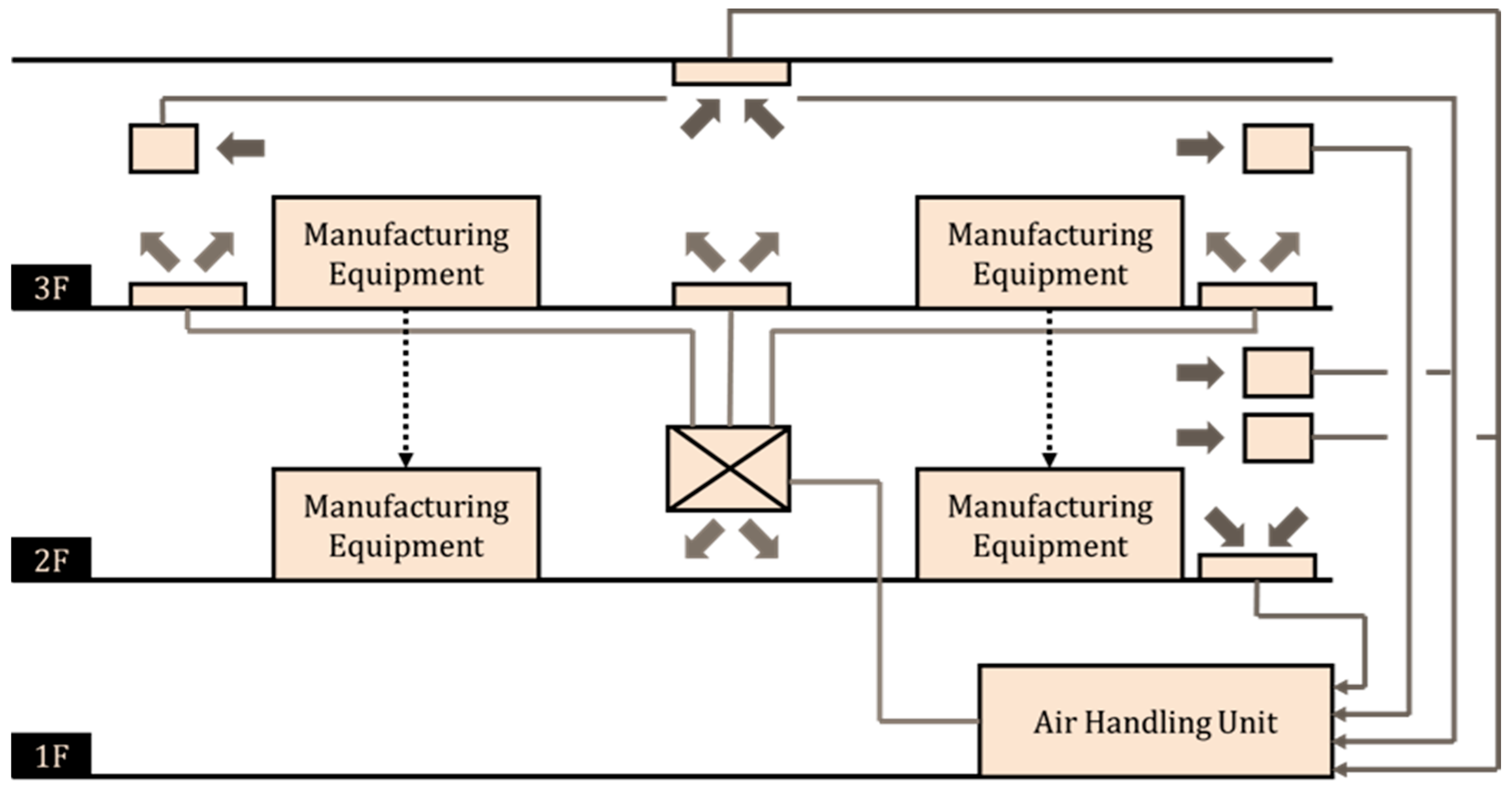
In a fiber chemical factory, for example, where environmental conditions play a crucial role in product quality, maintaining consistent air pressure is vital to stabilize operations and reduce downtime. This study aims to develop an intelligent, sensor-based autonomous control system to regulate air pressure differences, as shown in Figure 1. Adopting Industry 5.0 principles, the system integrates several layers of functionality, including actuator and sensor interfaces, process control, modeling, fault detection, and specification, to enhance human–machine collaboration. This approach involves designing sensor kits, deploying sensors, developing embedded systems, integrating IoT devices, and managing data through collection, integration, storage, and visualization techniques.
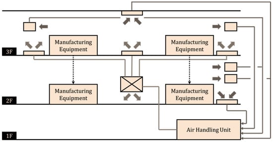
Figure 1.
HVAC system airflow diagram.
In Figure 1, the blank squares likely represent different zones or measurement points on each floor of the factory, while the cross within a square most probably depicts a central air handling component such as an Air Handling Unit (AHU). The lines illustrate the ductwork, with the blue lines and arrows indicating the path of supply air from the central unit to the floors, and the red lines and arrows showing the return air flowing back, while the dotted lines connect the manufacturing equipment to the floors to show the areas influenced by the HVAC system.
The concept of autonomy in manufacturing is rooted in the broader fields of cyber–physical systems (CPSs) and the Internet of Things (IoT), which enable the integration of physical processes with computational capabilities. This allows for the real-time monitoring and control of dynamic production environments, leading to systems that can adapt to complex production demands. Key developments in autonomy include the following:
- (1)
- Autonomous Production Control (APC): APC improves production performance by enabling fast, flexible responses to changes in the production environment. This approach decentralizes decision-making, transferring authority to distributed intelligent objects. While many studies on APC are theoretical, the practical applications are still limited.
- (2)
- Maturity Models for Autonomy: These models assess the level of autonomy in manufacturing systems, offering a framework for evaluating capabilities and pinpointing areas for improvement. The five-level autonomy model identifies the features and technologies required for each level.
- (3)
- Robotics: Autonomous robots are widely used in manufacturing for tasks such as assembly, welding, and material handling. These robots utilize advanced sensors and AI algorithms to perform tasks with high precision, enhancing production efficiency and reducing errors.
- (4)
- Process Automation: Autonomous control systems can automate entire production processes. Closed-loop AI systems adjust production parameters in real time based on sensor data, ensuring optimal performance while reducing waste.
- (5)
- Predictive Maintenance: By leveraging sensor data, autonomous systems can predict equipment failures and schedule maintenance proactively, leading to reduced downtime and increased equipment lifespan. Research demonstrates that predictive maintenance can result in significant cost savings.
Research on autonomous control systems continues to make strides in both theory and practice. While challenges remain, the potential benefits of enhanced efficiency, precision, safety, and cost savings make autonomous systems an asset in modern manufacturing. Our research focuses on overcoming technical barriers, addressing ethical considerations, and further developing autonomous systems to meet the evolving demands of the industry.
AI significantly enhances the capabilities of autonomous systems, driving innovation and efficiency across manufacturing processes. Some keyways AI influences these systems include the following:
- (1)
- Predictive Maintenance: AI algorithms analyze sensor data to predict equipment failures, reducing downtime and extending machinery lifespan by scheduling proactive maintenance.
- (2)
- Real-Time Monitoring and Control: AI systems process large volumes of sensor data in real time, making immediate adjustments to maintain optimal performance, ensuring smooth operations and higher product quality.
- (3)
- Generative Design: AI-driven generative design tools optimize designs based on specific requirements, creating lighter, stronger, and more cost-effective components.
- (4)
- Enhanced Robotics: AI improves autonomous robots’ capabilities, enabling them to perform complex tasks with greater precision and adaptability. These robots can learn from their environment and improve over time, making them more versatile.
- (5)
- Supply Chain Optimization: AI helps optimize supply chain management by predicting demand, managing inventories, and coordinating logistics. Autonomous systems with AI make real-time decisions, ensuring materials and products are available when needed.
- (6)
- Quality Control: AI-powered systems monitor product quality, detecting defects and making necessary adjustments in real time, ensuring that products meet stringent standards.
- (7)
- Human–Machine Collaboration: AI facilitates smoother collaboration between humans and machines, with autonomous systems managing repetitive or hazardous tasks, allowing human workers to focus on more complex and creative problem solving.
- (8)
- Adaptive Manufacturing: AI enables autonomous systems to adjust production parameters in real time based on sensor data and external factors, ensuring manufacturing processes remain responsive to changes in demand.
AI is transforming manufacturing by enhancing autonomous systems, improving efficiency, precision, and adaptability. As AI technology continues to evolve, its impact on autonomous systems will only grow, enabling smarter, more efficient factories in the future. The integration of digital twins and physical AI will further enhance these capabilities, driving a new era of manufacturing that is not only more efficient, but also more resilient, sustainable, and adaptable. While we build upon established concepts, our original contributions lie in the specific development, integration, and application of a human-centric autonomous HVAC control system tailored for the unique demands of chemical fiber manufacturing within the Industry 5.0 framework. Specifically, our novel contributions include the following:
The design and implementation of a multi-layered autonomous control architecture integrating edge AI, digital twins, and physical AI for HVAC control.
The development of specific AI models (NARX) incorporating airflow velocity data, which significantly improved predictive accuracy for indoor air pressure differences in this specific industrial setting (achieving R2 up to 0.9648 on test sets).
The design and deployment methodology for the sensor kits, including data collection via I2C, NTP synchronization, and OTA updates.
A demonstration of this integrated system in a real-world chemical fiber factory setting, focusing on human–machine collaboration aspects inherent to Industry 5.0. We have revised Section 1 and Section 5 to more explicitly highlight these original contributions and clearly differentiate our work from existing standards and protocols.
3. Methodology
Implementing an autonomous control system is a complex and detailed process that requires meticulous planning and precise execution. The initial phase involves designing the system by setting clear objectives, specifying necessary features, and selecting the appropriate technologies and algorithms. Following this, a reliable data collection platform must be developed, which includes choosing sensors and data acquisition systems that can efficiently and accurately gather the required data based on the system’s operational environment. The next step focuses on data storage and management, where selecting suitable database systems and data warehousing technologies is crucial to handling large volumes of data securely and effectively. Finally, the process involves system identification for neural network time-series analysis, which includes developing and training neural network models to analyze time-series data, recognize patterns, forecast future events, and adapt operations accordingly. This comprehensive approach ensures the successful implementation of an autonomous control system that is both efficient and adaptive.
3.1. Autonomous Control System Design
The autonomous control system architecture described consists of several functional layers:
- (1)
- Wind Sensors
These sensors measure wind speed and potentially other environmental factors. The raw data they generate is the foundation for the system, and it is transmitted to the next layer for processing.
- (2)
- Edge AI Processing
Located close to the sensors, edge AI performs preliminary data processing tasks. It filters, aggregates, and applies lightweight AI algorithms to the raw data. By processing data locally, the system reduces network traffic, minimizes latency, and allows for faster decision-making. This layer ensures only relevant, processed data moves upstream to the digital twins and central server.
- (3)
- Digital Twins
A digital twin is a virtual model of a physical system. Using the processed wind velocity data, the digital twin simulates real-world conditions, predicting future states (e.g., how wind velocity changes will affect airflow or temperature). The digital twin helps train AI models, refine predictions, and optimize system performance, ensuring better decision-making in future processes.
- (4)
- Neural Network pool
The neural network pool aggregates data from the digital twins and edge devices. It is responsible for heavier computational tasks such as refining AI models, conducting large-scale analytics, and storing historical data. The server uses insights from the digital twins to optimize control strategies, ensuring that decisions based on these models improve system efficiency and accuracy.
- (5)
- Factory Control System and HVAC System
The factory control system directly interacts with operational technology such as machinery, production lines, and other industrial equipment. It receives recommendations for control parameters (like airflow or temperature) from the digital twins and central server. The HVAC system, an example of a physical system, adjusts based on wind data and predictive models. These adjustments help optimize energy use, temperature regulation, and airflow. The feedback from these physical changes flows back to the sensors and edge AI, continually refining the system.
- (6)
- Physical AI
This layer represents the real-world application of digital insights. It includes hardware, robotics, and other industrial processes that execute the optimizations recommended by the AI-driven system. Physical AI takes the models and predictions from previous layers and directly influences machinery, airflow, and other physical aspects of the factory. This layer completes the feedback loop, with adjustments made in real time, leading to continuous optimization of the system.
This study employs a sophisticated computational framework for wind velocity prediction, with a critical component being the Wind Analytics module, as depicted in Figure 2. This module serves as the central processing hub for raw wind data, transforming it into a structured and informative format suitable for training the predictive models within the neural network pool.
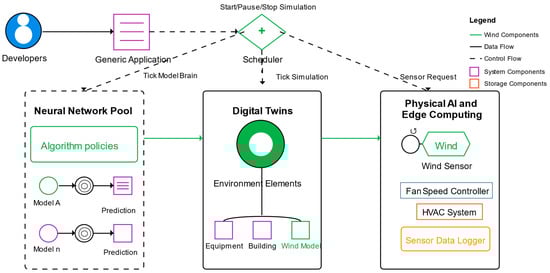
Figure 2.
The autonomous control system architecture and its components.
Upon receiving wind data from the physical AI and edge computing units, the Wind Analytics module initiates a series of crucial data processing steps. Firstly, data ingestion involves receiving a stream of wind measurements, including parameters such as wind velocity, wind direction, and potentially turbulence intensity, depending on the capabilities of the deployed wind sensors.
Following ingestion, the module undertakes rigorous data preprocessing. This stage typically involves several sub-processes aimed at ensuring data quality and consistency. Data cleaning addresses potential issues such as erroneous or outlier readings, which might arise due to sensor malfunctions or transient environmental events. Techniques like statistical outlier detection or range checks may be employed to identify and manage these anomalies. Furthermore, managing missing values is a critical step, as gaps in the data stream can negatively impact model training. Imputation techniques, such as using temporal interpolation or statistical averages, might be applied to fill these gaps appropriately. Data normalization or standardization is often performed to scale the different wind parameters to a common range, which can improve the convergence and performance of the machine learning algorithms.
A key function of the Wind Analytics module is feature engineering. This involves deriving new, potentially more informative features from the raw and pre-processed data. For instance, temporal features such as rolling averages, lagged values of wind speed, or directional changes over time might be calculated. Spatial features could also be incorporated if data from multiple wind sensors are available, allowing the module to capture spatial patterns and gradients in wind velocity. The selection and creation of relevant features are crucial for enhancing the predictive power of the subsequent machine learning models.
The culmination of these processing steps is the generation of Training Data. This involves structuring the processed and engineered features into a format suitable for supervised learning. Typically, this involves creating pairs of input features (e.g., historical wind data, environmental parameters) and corresponding target variables (e.g., future wind velocity at a specific location or time horizon). The Training Data are carefully partitioned into training, validation, and potentially testing sets to facilitate effective model training, hyperparameter tuning, and unbiased performance evaluation.
Beyond these core functions, the Wind Analytics module may also incorporate various analytical techniques to gain deeper insights into the wind patterns. This could involve statistical analysis, such as calculating descriptive statistics, identifying correlations between different wind parameters and environmental factors, or performing spectral analysis to understand the dominant frequencies in wind fluctuations. These analyses can inform the feature engineering process and provide valuable context for interpreting the model predictions.
The Training Data generated by the Wind Analytics module are then directly fed into the neural network pool. This curated and informative dataset is essential for effectively training the various predictive models (Model A to Model n), enabling them to learn the complex relationships between historical wind data, environmental conditions, and future wind velocity. The quality and relevance of the Training Data produced by the Wind Analytics module are therefore paramount to the overall accuracy and reliability of the wind velocity predictions generated by the framework.
3.2. Data Collection and Storage
Creating a platform for data collection that integrates multiple data sources is a complex but essential task in modern data-driven environments. Such a platform must be capable of handling diverse data types from various sources and making these data accessible for analysis and decision-making. One effective tool for this purpose is Node-RED, an open-source visual programming tool developed by IBM Emerging Technology. Node-RED allows users to wire together devices, Application Programming Interfaces (APIs), and online services by creating flows in a visual manner. It provides a browser-based flow editor where nodes represent different functionalities or devices. Users can connect these nodes to create a flow that processes, transforms, and routes data between various devices and services without extensive coding.
Node-RED offers several advantages that make it a preferred choice for system development, especially in the fields of Internet of Things (IoT) and data integration. Its flow-based programming paradigm allows users to create workflows by connecting pre-built nodes, representing specific functions, inputs, outputs, or devices, through a drag-and-drop interface. This simplifies the development process and makes it accessible to both beginners and experienced developers. Additionally, Node-RED has an extensive library of nodes covering a wide range of functionalities, including data processing, hardware integration, social media APIs, cloud services, and more. This versatility enables the creation of complex applications with contributions from the community and developers.
One of Node-RED’s strengths is its integration capabilities. It can seamlessly communicate with various systems and protocols, including MQTT, HTTP, TCP, UDP, WebSocket, databases, and IoT platforms. This interoperability facilitates the integration of different technologies, ensuring smooth data flow and communication. The browser-based interface of Node-RED further enhances its usability, allowing users to create, modify, and deploy flows using a visual editor. This accessibility streamlines the development process and makes it easier to manage and update the system.
For data storage, databases are essential as they provide structured collections of data organized to facilitate the efficient storage, retrieval, and manipulation of information. Databases serve as central repositories that store and manage vast amounts of structured, semi-structured, or unstructured data, providing a foundation for various applications and systems. Common classifications of databases include relational databases, NoSQL databases, and NewSQL databases. Relational databases, such as MySQL, PostgreSQL, Oracle, and SQL Server, organize data into tables with rows and columns, establishing relationships between different tables through keys. They use Structured Query Language (SQL) for querying and managing data and offer ACID (Atomicity, Consistency, Isolation, Durability) properties to ensure data integrity and consistency.
NoSQL databases, such as MongoDB, Redis, DynamoDB, Cassandra, and Neo4j, encompass various non-relational database models designed for scalability, flexibility, and handling unstructured or semi-structured data. They excel in distributed environments and offer schema flexibility and horizontal scaling. NewSQL databases, like Google Spanner, CockroachDB, and VoltDB, combine aspects of relational databases with the scalability of NoSQL, addressing the limitations of traditional SQL databases concerning scalability and performance while retaining ACID compliance.
InfluxDB is a popular open-source time-series database designed to handle high write and query loads, making it particularly well suited for applications that require handling time-stamped data. Its design is optimized for time-series data, offering high performance in data ingestion and query processing, which is essential for applications relying on rapid data collection and real-time analysis. InfluxDB’s query language is intuitively like SQL, making it accessible to individuals accustomed to traditional database languages. Its scalability allows it to accommodate growing data volumes and increasingly complex queries without compromising performance. Additionally, InfluxDB is user-friendly, offering straightforward setup and maintenance operation. These features make InfluxDB an ideal choice for research and applications requiring efficient and scalable time-series data management.
In summary, creating a data collection platform that integrates multiple data sources involves selecting the right tools and technologies to handle diverse data types, ensure seamless integration, and provide efficient data storage and management. Node-RED and InfluxDB are powerful tools that offer the necessary capabilities to build a robust and scalable data collection platform, facilitating real-time analysis and decision-making.
3.3. System Identification
System identification is a field of study in engineering that aims to build mathematical models of dynamic systems from the observed input–output data [40]. It involves inferring the underlying structure, behavior, and dynamics of a system based on observed inputs and outputs, enabling analysis, prediction, control, and optimization. The primary goal is to develop accurate and reliable models that allow for a better understanding and manipulation of complex systems.
Mathematical modeling for system identification employs various techniques, including differential equations, transfer functions, state-space models, and time-series models. Parameter estimation techniques, such as least squares estimation, maximum likelihood estimation, and Bayesian estimation, are used to estimate the parameters of these mathematical models based on observed data.
System identification relies on high-quality data and data preprocessing techniques to manage noise, outliers, and missing values. Complex models might also lead to overfitting; thus, model validation techniques like cross-validation are adopted to ensure generalizability and accuracy. To classify different complexities of systems, the following features are considered:
- (1)
- Linear and Nonlinear Systems: Linear systems have linear relationships between inputs and outputs, whereas nonlinear systems have more complex, non-linear relationships.
- (2)
- Time-Invariant and Time-Varying Systems: Time-invariant systems have properties that do not change over time, while time-varying systems exhibit variations or changes in their characteristics.
- (3)
- Parametric and Nonparametric Methods: Parametric methods assume a specific model structure with defined parameters, while nonparametric methods do not make assumptions about the model structure.
System identification methodologies are often categorized into “White Box”, “Grey Box”, and “Black Box” approaches:
- (1)
- White Box Models: These models are based on theoretical knowledge of the system. They are highly interpretable but can be limited by the accuracy of theoretical knowledge.
- (2)
- Grey Box Models: These models combine theoretical knowledge with data-driven approaches, offering a balance between interpretability and flexibility.
- (3)
- Black Box Models: These models are developed purely from input–output data, often relying on complex algorithms or artificial intelligence. They can capture complex dynamics but may lack interpretability and require large amounts of data.
Time-series analysis involves analyzing and predicting future values based on historical data points collected at regular intervals over time. Neural networks have emerged as powerful tools for handling time-series data due to their ability to model complex patterns and dependencies within sequential data. However, neural networks also face challenges, such as overfitting, interpretability, and the need for large datasets.
The Nonlinear AutoRegressive eXogenous (NARX) model is a dynamic nonlinear model used in time-series analysis and system identification. It extends the conventional AutoRegressive eXogenous (ARX) model by incorporating nonlinear functions of the input and output variables. In the NARX model, the current output depends not only on past inputs and outputs, but also on delayed and nonlinear transformations of these variables. This model is represented by a nonlinear function of lagged inputs and outputs, as well as potentially exogenous variables, allowing for the capture of complex relationships and nonlinear dynamics within the data.
Implementing NARX models involves data preprocessing, model selection, and training procedures. Data preprocessing includes feature engineering to extract meaningful information from time-series data. Model selection involves determining the optimal lag order and number of neurons, selecting relevant input variables, and choosing appropriate nonlinear functions or basis functions. Training the NARX model involves optimization techniques such as gradient-based optimization, least squares, or nonlinear optimization methods to estimate the model parameters.
The NARX model stands out for its adaptability and precision in handling complex data patterns, especially for nonlinear systems. The effectiveness of the black box approach lies in the ability to experiment with various input and output combinations, allowing for a comprehensive comparison and evaluation of the model’s performance across a range of scenarios. By systematically varying the inputs, outputs, time delay, and number of neurons, it becomes possible to discern the most effective configuration for the model, thereby optimizing both accuracy and reliability in its predictions.
Autocorrelation is a foundational concept in time-series analysis, offering crucial insights into the relationship between observations over time. It measures the degree of similarity between a sequence of data points and its lagged versions, essentially examining how closely a data point relates to its past observations at different time intervals or lags. This analysis unveils patterns, dependencies, and structures inherent in sequential data, aiding in understanding trends, seasonality, and underlying temporal dynamics.
The autocorrelation function (ACF) quantifies the correlation between a time series and its lagged versions. Mathematically, for a time series () with observations at discrete time points (t), the autocorrelation at lag (k) is calculated using the following formula:
Here, n represents the total number of observations, k is the lag or time interval, denotes the data point at time t, and the mean of the time series is represented by .
The ACF provides insights into the correlation structure of a time series across different lags. Positive autocorrelation at lag (k) indicates that data points separated by (k) time intervals are positively correlated, while negative autocorrelation suggests an inverse relationship. ACF values close to zero imply weak or no correlation at that lag. Detecting autocorrelation assists in model selection for time-series forecasting, such as in AutoRegressive Integrated Moving Average (ARIMA) models, where the ACF and partial autocorrelation function (PACF) guide the selection of model parameters. Understanding autocorrelation and its statistical analysis enables analysts to discern temporal relationships within data, aiding in model selection, validation, and forecasting.
A specific type of air velocity sensor was chosen to measure airflow velocity in various environments, and its specifications are listed in Table 1. To ensure accurate and reliable data collection, several designs for sensor deployment have been developed. These designs include sensor Printed Circuit Boards (PCBs) and sensor mounting devices, each tailored to the specific requirements of different deployment locations. For instance, some sensors may be mounted on walls, ceilings, or other structures depending on the area being monitored.

Table 1.
General specifications of F660.
The F660 sensor manufactured by DEGREE CONTROLS, INC, Nashua, New Hampshire, USA, operates within a temperature range of 0 °C to 60 °C and can be stored between −40 °C and 105 °C. It functions effectively in relative humidity levels of 5% to 95% (non-condensing), has a response time of 400 milliseconds, features a configurable trip point output, supports 3.3 V I2C at 400 kHz or 3.3 VDC UART for communications, is housed in flame-retardant Nylon UL94-V0 material, operates ideally within a voltage range of 15–18 VDC (recommended 12–24 VDC), offers a resolution of 0.1 °C, and weighs 2.5 g, as shown in Table 1.
The air velocity accuracy within the compensation range is ±(5% of reading + 0.04 m/s) for air velocities between 0.15 m/s and 1.0 m/s, ±(5% of reading + 0.10 m/s) for air velocities between 0.5 m/s and 10 m/s, and ±(5% of reading + 0.15 m/s) for air velocities between 1.0 m/s and 20 m/s, as shown in Table 2.
Table 2.
Air velocity accuracy.
Each sensor kit is equipped with a microcontroller that collects [21] multiple sensor readings using the Inter-Integrated Circuit (I2C) protocol. The I2C protocol is a popular communication standard that allows multiple sensors to communicate with the microcontroller efficiently. This setup ensures that data from various sensors can be gathered simultaneously and accurately.
To maintain synchronization and ensure the accuracy of the collected data, the microcontroller uses a Network Time Protocol (NTP) server. The NTP server provides precise timekeeping, allowing the microcontroller to timestamp each data reading accurately. This synchronization is crucial for analyzing trends and patterns in the airflow data over time.
Additionally, the microcontroller is equipped with an Over-The-Air (OTA) firmware update feature. This feature allows for remote updates of the microcontroller’s firmware, ensuring that the system can be easily maintained and upgraded without the need for physical access. OTA updates are essential for version control and for implementing improvements or bug fixes in the system.
Once the data have been collected by the microcontroller, they are organized and processed for visualization. The data can be displayed in trend charts, which show changes in airflow velocity over time, or on customized web pages that provide a more detailed and interactive view of the data. These visualizations help users understand the airflow patterns and make informed decisions based on the collected data.
In summary, the deployment of air velocity sensors involves careful planning and design to ensure accurate data collection. The use of microcontrollers with I2C communication, NTP synchronization, and OTA firmware updates enhances the reliability and maintainability of the system. The collected data are then visualized in various formats to provide valuable insights into airflow dynamics, as will be demonstrated in the following sections.
3.4. Data Selection and Preprocessing
For predicting indoor air pressure differences, the key features selected include AHU output, airflow velocity, and indoor air pressure differences. Each feature contains 66,475 sets of raw data with a time interval of 1 min. The data are summarized in Table 3.
Table 3.
Modeling data.
Data preprocessing is crucial for improving data quality and making it suitable for analysis. The following techniques were applied:
- (1)
- Filling Missing Data: Missing data were addressed using linear interpolation, which estimates values within the range of known data points. This method ensures the continuity and completeness of the dataset.
- (2)
- Cleaning Outliers: Outliers were identified and managed using the moving median technique. This method is effective for time-series data as it is less sensitive to outliers compared to the moving average.
- (3)
- Data Normalization: Z-score normalization was applied to adjust the range of data values to a common scale. The Z-score is calculated using the following formula:
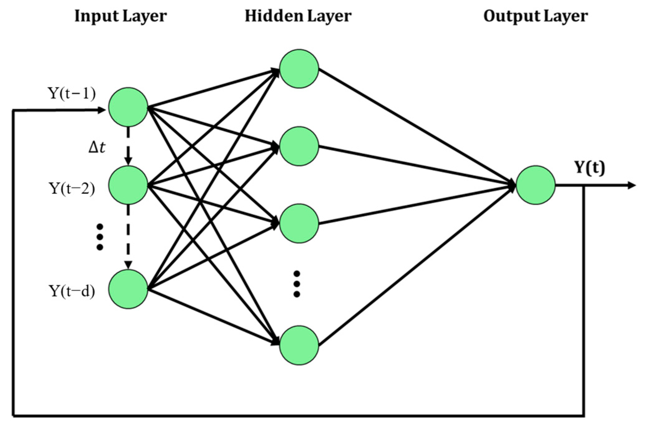
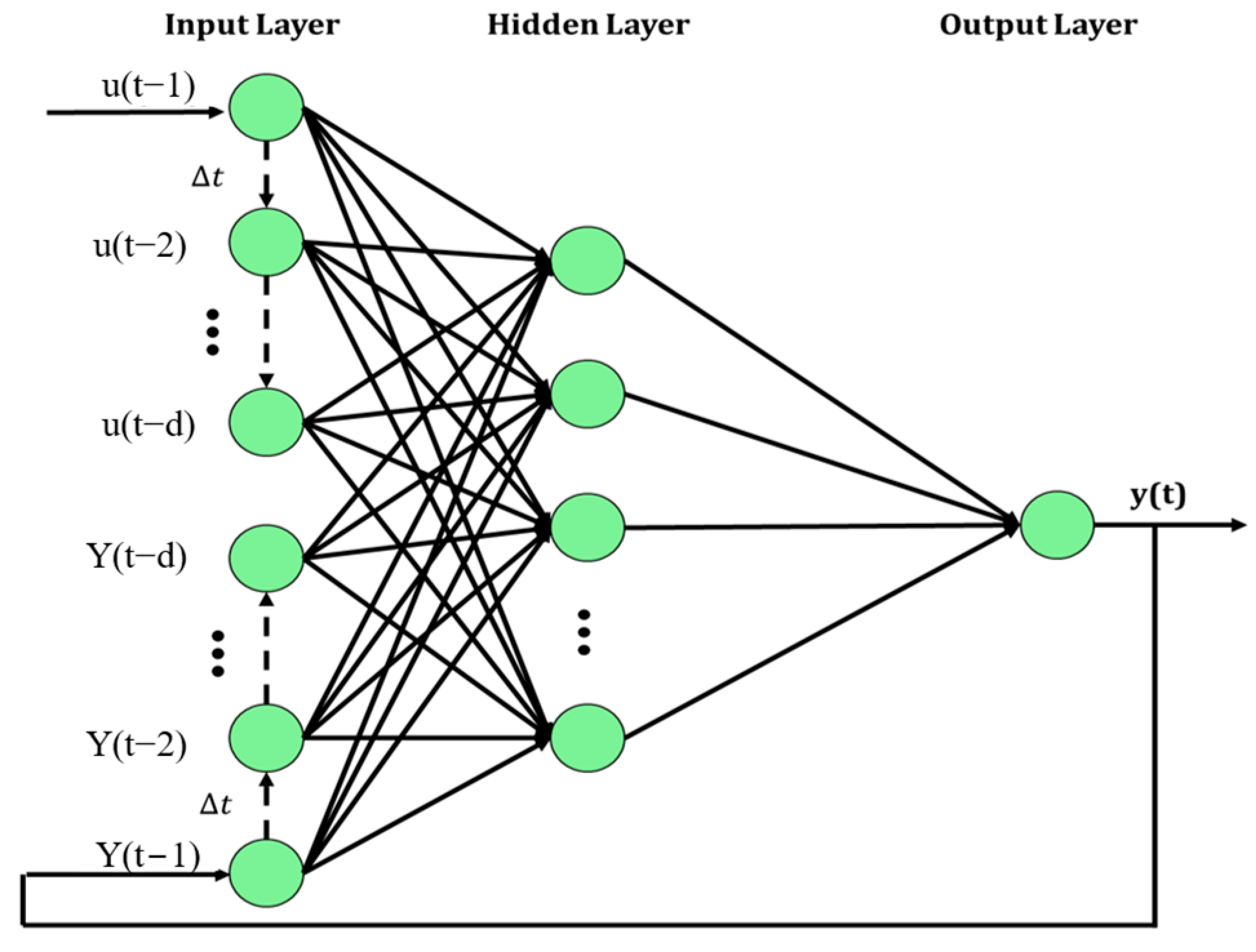
Two model structures were compared: NAR (Nonlinear AutoRegressive) and NARX (Nonlinear AutoRegressive with eXogenous inputs). The NAR model uses past values of ) to predict , while the NARX model uses past values of and another series to predict , as shown in Figure 3 and Figure 4.
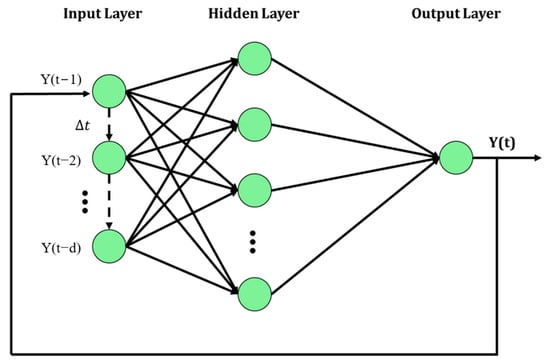
Figure 3.
Structure of NAR model (d represents the time delay).

Figure 4.
Structure of NARX model (d represents the time delay).
Model training involves iterating different parameters to minimize the loss function, which quantifies the accuracy of the model’s predictions. The performance of each model was assessed based on the average value, calculated from training the model five times.
- -
- Model A: Uses past values of indoor air pressure differences to predict future values with an NAR structure. Optimal performance was achieved with a layer size of 20 and a time delay of 30.
- -
- Model B: Uses past values of AHU output and indoor air pressure differences to predict future values with an NARX structure. Optimal performance was achieved with a layer size of 10 and a time delay of 5. It is important to clarify that Section 3 presents a conceptual framework intended to guide the design and development of the autonomous control system, rather than describing a fully implemented system with a complete operational interface. Our objective at this stage was to propose a generalizable architecture and control logic to support future implementations. For future development, we believe Node-RED would be a suitable platform for creating a user-friendly interface that supports real-time monitoring, control input, and system visualization.
This comprehensive approach ensures accurate and reliable predictions of indoor air pressure differences, leveraging advanced data preprocessing and model training techniques. While the system is designed for autonomous air pressure regulation, its human-centric nature, central to Industry 5.0, is realized through several integrated features: the “specification” level allows human operators to define system objectives and requirements, ensuring that the autonomous operation aligns with human needs and priorities; the real-time monitoring web application and detailed data visualization tools provide operators with transparency into the system’s performance and environmental conditions, enabling informed oversight, trust, and the ability to intervene or adjust specifications; moreover, by maintaining the precise environmental control crucial for product quality and worker safety, the system directly enhances the human work environment, acting as a collaborative partner that augments human capabilities and well-being rather than merely automating tasks.
4. Results and Discussion
This study investigates the prediction of indoor air pressure differences using various machine learning models, focusing on the impact of predictor selection and model configuration. The core objective is to minimize the loss function by optimizing model parameters, thereby enhancing prediction accuracy. Specifically, this involved tuning the structural configuration of the neural network models by varying the layer size (number of neurons in the hidden layer) and the temporal configuration by adjusting the time delay (number of past time steps considered).
Four model approaches were evaluated:
- Model A (NAR): Utilized past indoor air pressure differences to predict future values.
- Model B (NARX): Incorporated past AHU output and past indoor air pressure differences.
- Model C (NARX): Employed past airflow velocity and past indoor air pressure differences.
- Model D (NARX): Combined past AHU output, past airflow velocity, and past indoor air pressure differences.
Model performance was assessed using the average R2 value across five training iterations. The impact of layer size and time delay was systematically examined for each model.
- (1)
- Model A
Model A directly uses past values of indoor air pressure differences to predict indoor air pressure differences with an NAR model structure. Model A had a better performance when the layer size was set to 20 and time delay was set to 30, as shown in Table 4 and Table 5.
Table 4.
Model A: Performance evaluation across layer-size iterations.
Table 5.
Model A: Performance evaluation across time-delay iterations.
- (2)
- Model B
Model B employs an NARX model structure, using past values of AHU outputs and past values of indoor air pressure differences to predict indoor air pressure differences. As indicated in Table 6 and Table 7, Model B demonstrated improved performance with the layer size configured at 10 and the time delay set to 5.
Table 6.
Model B: Performance evaluation across layer-size iterations.
Table 7.
Model B: Performance evaluation across time-delay iterations.
- (3)
- Model C
Model C adopts an NARX model structure, utilizing previous airflow velocity and previous indoor air pressure differences to predict indoor air pressure differences. Table 8 and Table 9 show that Model C’s performance was enhanced when it was configured with a layer size of 10 and a time delay of 5.
Table 8.
Model C: Performance evaluation across layer-size iterations.
Table 9.
Model C: Performance evaluation across time-delay iterations.
- (4)
- Model D
Model D uses past values of AHU output, past values of airflow velocity, and past values of indoor air pressure differences to predict indoor air pressure differences with an NARX model structure. Table 10 and Table 11 reveal that Model D exhibited enhanced performance when set with a layer size of 10 and a time delay of 5.
Table 10.
Model D: Performance evaluation across layer-size iterations.
Table 11.
Model D: Performance evaluation across time-delay iterations.
By integrating the optimal configurations for both layer size and time delay, as determined by the R2 value, the top model candidates are enumerated in Table 12.
Table 12.
Top model candidates.
Next, we used an additional test set (i.e., subset 2 to 5) to check the performance of the above models. The results are shown in Table 13.
Table 13.
Additional test for models.
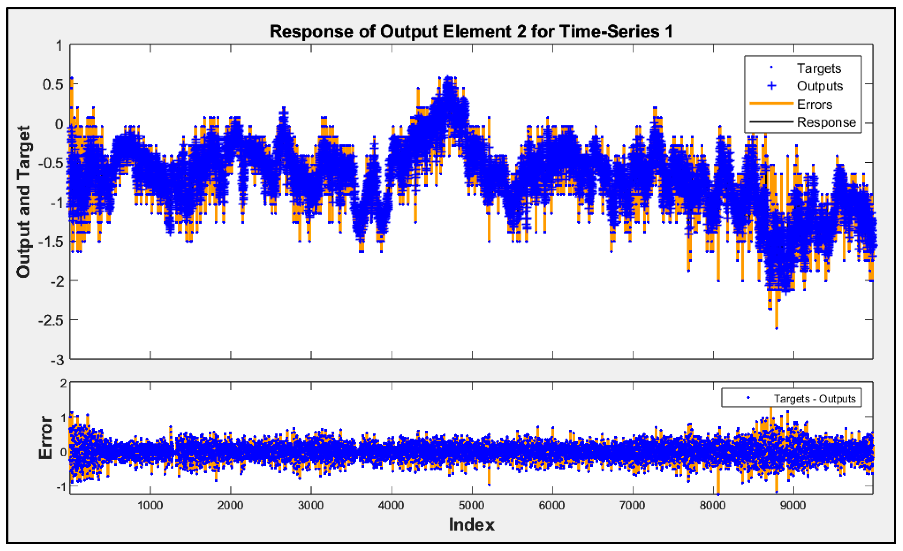
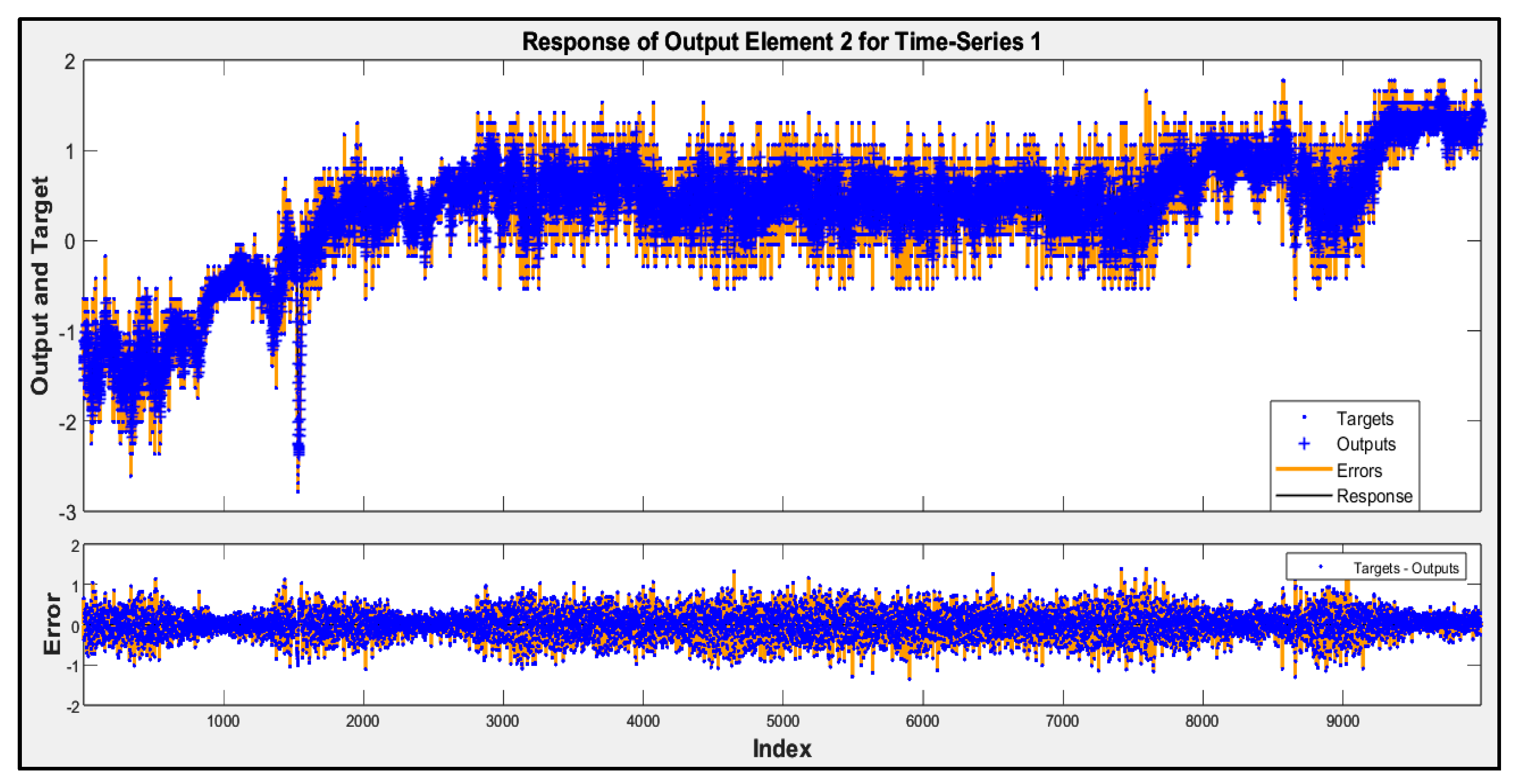
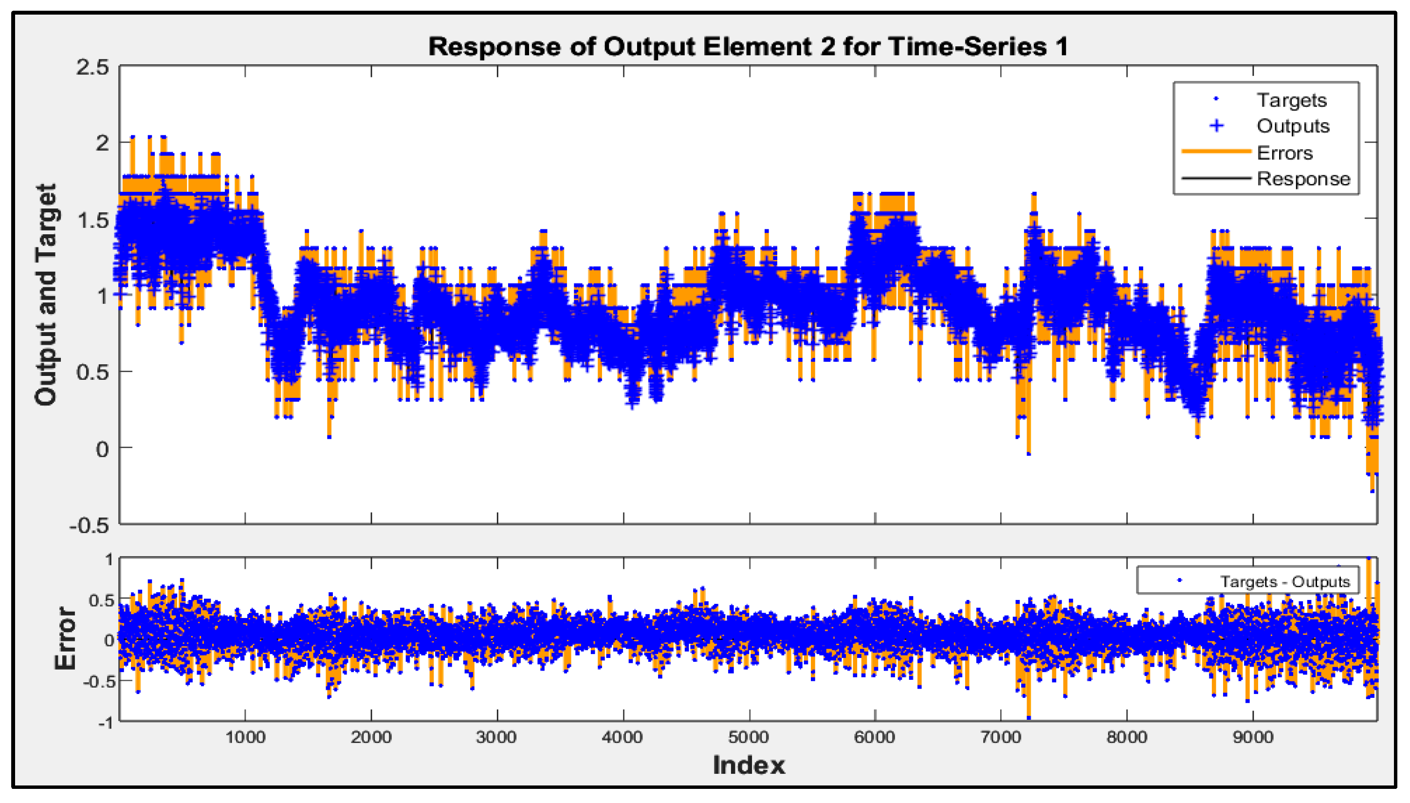
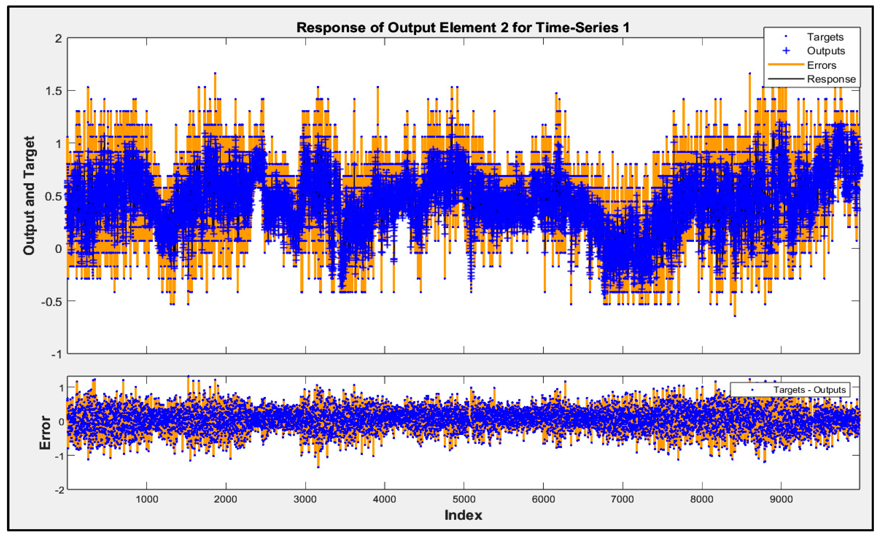
Involving airflow velocity in the prediction models significantly enhanced their accuracy and contributed to more consistent performance across future data subsets. The predicted responses from Model D for subsets 2 to 5 are shown in Figure 5, Figure 6, Figure 7 and Figure 8. These figures display the actual performance of Model D, which incorporates airflow velocity data, on four separate test datasets (subsets 2–5). In the upper plot of each figure, the blue dots represent the real, measured indoor air pressure differences (the “Targets”). The orange line shows the values predicted by Model D (the “Outputs”). Observing how closely the orange line follows the pattern of the blue dots across the entire time series in each figure directly illustrates the model’s predictive accuracy on that specific subset of unseen data. A tight alignment between the orange line and the blue dots, as is generally visible in these figures, indicates that the model’s predictions closely match the actual measured values. The lower plot in each figure shows the “Error”, which is the difference between the actual target and the predicted output. The distribution of these error points around the zero line indicates the magnitude and variability of the prediction errors. The fact that most error points are relatively close to the zero line across all four subsets visually supports the quantitative R2 values and demonstrates that Model D is able to generalize its predictive capability effectively to new, unseen data, reinforcing the benefit of including airflow velocity as a predictor.
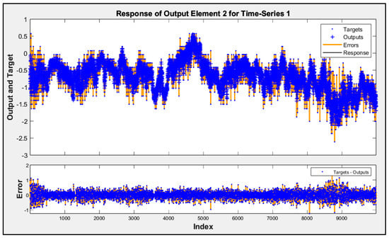
Figure 5.
Time-series response analysis of subset 2.

Figure 6.
Time-series response analysis of subset 3.
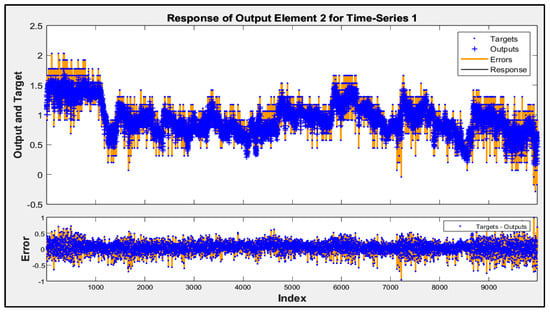
Figure 7.
Time-series response analysis of subset 4.
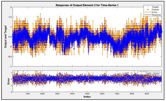
Figure 8.
Time-series response analysis of subset 5.
Autocorrelation of residuals is a statistical technique used in various fields, particularly in time-series analysis. Its primary purpose is to assess whether the residuals (or errors) from a model exhibit autocorrelation. Autocorrelation indicates a systematic pattern of correlation between the error terms at different time points or lags. When the prediction error is obviously autocorrelated, then the prediction error is dependent on the time series.
The autocorrelation plots for the errors of Model D from subsets 1 to 5 are shown in Figure 9a–e. The plots’ horizontal axes depict lag values, signifying the time interval by which the error terms are compared. For instance, lag 1 compares consecutive error terms, lag 2 assesses error terms separated by two time points, and so forth. On the other hand, the vertical axis on the plot displays autocorrelation coefficients, quantifying the magnitude and direction of correlation among error terms at the chosen lag. For a perfect prediction model, there should only be one non-zero value of the autocorrelation function that occurs at zero lag. This occurrence signifies that the prediction errors are entirely uncorrelated, resembling white noise.
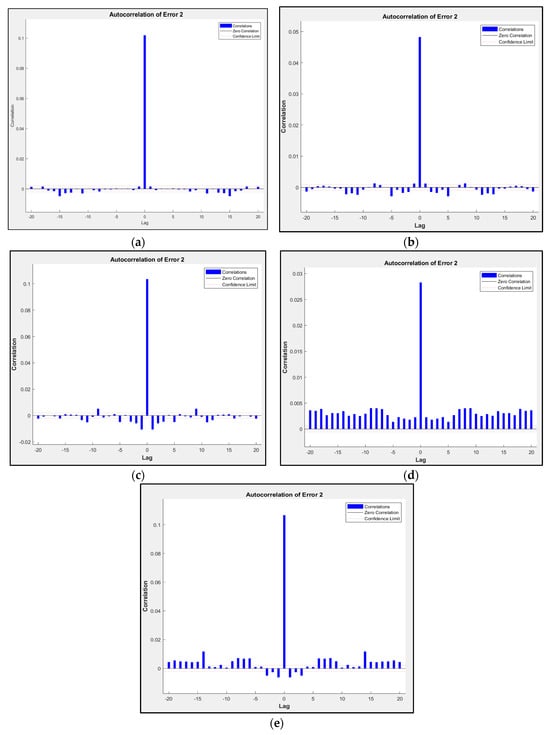
Figure 9.
Autocorrelation plot for subsets: (a) subset 1; (b) subset 2; (c) subset 3; (d) subset 4; (e) subset 5.
The autocorrelation plot above demonstrates that as we move further back in time, within-dataset errors become more correlated. This suggests that there is an opportunity for improvement through a retraining process, potentially by adjusting the layer size or increasing the number of time delays in the model settings.
The implementation of autonomous control systems has significantly improved operational efficiency by reducing the need for experts to perform repetitive tasks. However, these systems face a critical challenge known as model decay, where their performance diminishes over time due to changes in the environment or data. Model decay occurs primarily due to concept drift (when the meaning of data changes over time) and data drift (when models trained on specific data periods fail to perform as well on data from other periods).
To address model decay, strategies like error autocorrelation analysis can help identify performance deviations, prompting the need for model retraining. This analysis acts as a “critic”, triggering a retraining process when correlated errors indicate that a model is no longer performing optimally. Additionally, fault detection mechanisms are crucial in preventing model decay, particularly by identifying and correcting sensor deviations, ensuring that the model receives accurate data inputs and maintains reliability.
In the future, integrating a neural network controller into the autonomous system could improve its ability to adapt to real-time data and dynamic environments. Unlike traditional simulation models, prediction models use current data to forecast the system’s response in the next time step, which could be beneficial for fine-tuning the controller’s performance. Neural network predictive controllers could optimize plant performance by predicting future behavior and adjusting control inputs accordingly. Testing and optimizing such controllers would require either a real plant with a prediction model or a fully functional simulation model to ensure their effectiveness in actual operational conditions.
5. Conclusions
This study successfully developed and implemented a novel human-centric autonomous control system specifically tailored for an HVAC system within a chemical fiber manufacturing facility, operating within the principles of Industry 5.0. The core objective was to accurately predict indoor air pressure differences, a critical parameter for maintaining product quality and worker safety in this specific industrial environment. The system’s architecture is multi-layered, designed to facilitate seamless data acquisition from distributed sensor kits, efficient data management and streaming, and intuitive visualization for human operators [41]. This integrated approach underscores Industry 5.0’s focus on augmenting human capabilities through advanced technology and fostering effective human–machine collaboration. A significant contribution of this research lies in the application of AI-driven system identification using Nonlinear AutoRegressive with eXogenous inputs (NARX) models. Through rigorous analysis, it was empirically demonstrated that the inclusion of airflow velocity data as an exogenous input significantly improved the predictive accuracy of the model for indoor air pressure differences. This finding is particularly relevant for industrial settings where environmental factors like air movement play a crucial role, highlighting the importance of selecting appropriate input variables for data-driven models to achieve high performance. Furthermore, the implemented system incorporates a vital retraining workflow designed to counteract the phenomenon of model decay, which is a common challenge in dynamic industrial environments where conditions can change over time. This workflow currently utilizes error autocorrelation analysis as a trigger mechanism, prompting the system to retrain the predictive model when the prediction errors exhibit a systematic pattern, indicating that the model is no longer accurately capturing the system’s dynamics. While this method ensures ongoing model fitness, a recognized limitation is the potential for delays in detecting subtle shifts or the need for more sophisticated triggers that can anticipate decay more proactively. Building upon the success of this framework, future research will focus on further enhancing the system’s capabilities. A key direction involves integrating a neural network controller. This integration is envisioned to leverage accurate predictions from the NARX model to enable more dynamic and precise real-time adjustments to the HVAC system, thereby optimizing performance and maintaining desired air pressure differentials more effectively. The successful implementation and validation of such a controller will require comprehensive testing, either within the operational chemical fiber factory environment or through the development of highly accurate and representative simulation models. This continued development is crucial for advancing towards the creation of truly resilient, adaptive, and highly efficient industrial control systems that fully embody the potential of Industry 5.0.
Author Contributions
Conceptualization, M.B. and J.-S.S.; methodology, J.C. and R.C.; validation, M.B. and J.C.; formal analysis, R.C.; investigation, M.B. and J.C.; resources, J.-S.S.; data curation, J.C.; writing—original draft preparation, M.B.; writing—review and editing, J.-S.S. and R.C.; visualization, J.C.; supervision, J.-S.S.; project administration, J.-S.S. All authors have read and agreed to the published version of the manuscript.
Funding
This study was financially supported by the National Science and Technology Council, Taiwan (grant number: NSTC 112-2221-E-155-001).
Data Availability Statement
The original contributions presented in this study are included in the article. Further inquiries can be directed to the corresponding author.
Conflicts of Interest
The author Rick Chen was employed by the Far Eastern Fibertech Company Limited. The remaining authors declare that the research was conducted in the absence of any commercial or financial relationships that could be construed as a potential conflict of interest.
References
- Adel, A. Unlocking the future: Fostering human–machine collaboration and driving intelligent automation through industry 5.0 in smart cities. Smart Cities 2023, 6, 2742–2782. [Google Scholar] [CrossRef]
- Verma, R.C.; Chaurasiya, S.; Kumar, A. Human-Machine Collaboration in Smart Factories: A Transition from Industry 4.0 to Industry 5.0. Int. J. Cult. Stud. Soc. Sci. 2024, 20, 149–158. [Google Scholar]
- Martini, B.; Bellisario, D.; Coletti, P. Human-centered and sustainable artificial intelligence in industry 5.0: Challenges and perspectives. Sustainability 2024, 16, 5448. [Google Scholar] [CrossRef]
- Yang, Y.; Keivanpour, S.; Imbeau, D. The Future of Disassembly Planning: A Critical Assessment of Industry 5.0, Lean, and X-Reality. In Proceedings of the 2023 International Conference on Electrical, Computer and Energy Technologies (ICECET), Cape Town, South Africa, 16–17 November 2023; IEEE: Piscataway, NJ, USA; pp. 1–12. [Google Scholar]
- Elsaid, A.M.; Mohamed, H.A.; Abdelaziz, G.B.; Ahmed, M.S. A critical review of heating, ventilation, and air conditioning (HVAC) systems within the context of a global SARS-CoV-2 epidemic. Process Saf. Environ. Prot. 2021, 155, 230–261. [Google Scholar] [CrossRef] [PubMed]
- Alam, M.A.; Kumar, R.; Yadav, A.S.; Arya, R.K.; Singh, V. Recent developments trends in HVAC (heating, ventilation, and air-conditioning) systems: A comprehensive review. Mater. Today Proc. 2023, in press. [Google Scholar] [CrossRef]
- Yao, Y.; Shekhar, D.K. State of the art review on model predictive control (MPC) in Heating Ventilation and Air-conditioning (HVAC) field. Build. Environ. 2021, 200, 107952. [Google Scholar] [CrossRef]
- Bhat, S. Building Thermal Comforts with Various HVAC Systems and Optimum Conditions. Int. J. Multidiscip. Res. Sci. Eng. Technol. 2024, 7, 14845–14852. [Google Scholar]
- Shi, Y.; Liu, M.; Fang, F. Combined Cooling, Heating, and Power Systems: Modeling, Optimization, and Operation; Wiley: Hoboken, NJ, USA, 2017. [Google Scholar]
- Lopez-Carreon, I.; Jahan, E.; Yari, M.H.; Esmizadeh, E.; Riahinezhad, M.; Lacasse, M.; Xiao, Z.; Dragomirescu, E. Moisture Ingress in Building Envelope Materials: (II) Transport Mechanisms and Practical Mitigation Approaches. Buildings 2025, 15, 762. [Google Scholar] [CrossRef]
- Okochi, G.S.; Yao, Y. A review of recent developments and technological advancements of variable-air-volume (VAV) air-conditioning systems. Renew. Sustain. Energy Rev. 2016, 59, 784–817. [Google Scholar] [CrossRef]
- Asim, N.; Badiei, M.; Mohammad, M.; Razali, H.; Rajabi, A.; Chin Haw, L.; Jameelah Ghazali, M. Sustainability of heating, ventilation and air-conditioning (HVAC) systems in buildings—An overview. Int. J. Environ. Res. Public Health 2022, 19, 1016. [Google Scholar] [CrossRef]
- Larsen, T.S.; Heiselberg, P. Single-sided natural ventilation driven by wind pressure and temperature difference. Energy Build. 2008, 40, 1031–1040. [Google Scholar] [CrossRef]
- Kimla, J. Optimized Fan Control in Variable Air Volume HVAC Systems Using Static Pressure Resets: Strategy Selection and Savings Analysis. Master’s Thesis, Texas A&M University, College Station, TX, USA, 2010. [Google Scholar]
- Zizic, M.C.; Mladineo, M.; Gjeldum, N.; Celent, L. From industry 4.0 towards industry 5.0: A review and analysis of paradigm shift for the people, organization and technology. Energies 2022, 15, 5221. [Google Scholar] [CrossRef]
- Xu, M.; David, J.M.; Kim, S.H. The fourth industrial revolution: Opportunities and challenges. Int. J. Financ. Res. 2018, 9, 90–95. [Google Scholar] [CrossRef]
- De Vries, J. The industrial revolution and the industrious revolution. J. Econ. Hist. 1994, 54, 249–270. [Google Scholar] [CrossRef]
- Verma, A. Introduction to autonomous systems. In Handbook of Power Electronics in Autonomous and Electric Vehicles, Elsevier: Amsterdam, The Netherlands, 2024; pp. 17–28.
- Arya, S.S.; Dias, S.B.; Jelinek, H.F.; Hadjileontiadis, L.J.; Pappa, A.-M. The convergence of traditional and digital biomarkers through AI-assisted biosensing: A new era in translational diagnostics? Biosens. Bioelectron. 2023, 235, 115387. [Google Scholar] [CrossRef]
- Pansare, P. Smart Cities Using Green Computing: A Citizen Data Scientist Perspective. In Green Computing for Sustainable Smart Cities; CRC Press: Boca Raton, FL, USA, 2024; pp. 341–368. [Google Scholar]
- Mourtzis, D.; Angelopoulos, J. Artificial intelligence for human–cyber-physical production systems. In Manufacturing from Industry 4.0 to Industry 5.0; Elsevier: Amsterdam, The Netherlands, 2024; pp. 343–378. [Google Scholar]
- Omol, E.; Mburu, L.; Onyango, D. Anomaly detection in IoT sensor data using machine learning techniques for predictive maintenance in smart grids. Int. J. Sci. Technol. Manag. 2024, 5, 201–210. [Google Scholar] [CrossRef]
- Syafrudin, M.; Alfian, G.; Fitriyani, N.L.; Rhee, J. Performance analysis of IoT-based sensor, big data processing, and machine learning model for real-time monitoring system in automotive manufacturing. Sensors 2018, 18, 2946. [Google Scholar] [CrossRef] [PubMed]
- Pereira, C.E.; Carro, L. Distributed real-time embedded systems: Recent advances, future trends and their impact on manufacturing plant control. Annu. Rev. Control 2007, 31, 81–92. [Google Scholar] [CrossRef]
- Wanner, J.P. Artificial Intelligence for Human Decision-Makers: Systematization, Perception, and Adoption of Intelligent Decision Support Systems in Industry 4.0. Ph.D. Dissertation, Universität Würzburg, Würzburg, Germany, 2022. [Google Scholar]
- Newman, D.; Blanchard, O. Human/Machine: The Future of Our Partnership with Machines; Kogan Page Publishers: London, UK, 2019. [Google Scholar]
- Javaid, M.; Haleem, A.; Suman, R. Digital twin applications toward industry 4.0: A review. Cogn. Robot. 2023, 3, 71–92. [Google Scholar] [CrossRef]
- Jiang, H.; Qin, S.; Fu, J.; Zhang, J.; Ding, G. How to model and implement connections between physical and virtual models for digital twin application. J. Manuf. Syst. 2021, 58, 36–51. [Google Scholar] [CrossRef]
- Nikolakis, N.; Alexopoulos, K.; Xanthakis, E.; Chryssolouris, G. The digital twin implementation for linking the virtual representation of human-based production tasks to their physical counterpart in the factory-floor. Int. J. Comput. Integr. Manuf. 2019, 32, 1–12. [Google Scholar] [CrossRef]
- Sharma, A.; Kosasih, E.; Zhang, J.; Brintrup, A.; Calinescu, A. Digital Twins: State of the art theory and practice, challenges, and open research questions. J. Ind. Inf. Integr. 2022, 30, 100383. [Google Scholar] [CrossRef]
- Omrany, H.; Al-Obaidi, K.M.; Husain, A.; Ghaffarianhoseini, A. Digital twins in the construction industry: A comprehensive review of current implementations, enabling technologies, and future directions. Sustainability 2023, 15, 10908. [Google Scholar] [CrossRef]
- Kritzinger, W.; Karner, M.; Traar, G.; Henjes, J.; Sihn, W. Digital Twin in manufacturing: A categorical literature review and classification. Ifac-Pap. 2018, 51, 1016–1022. [Google Scholar] [CrossRef]
- Boschert, S.; Rosen, R. Digital twin—The simulation aspect. In Mechatronic Futures: Challenges and Solutions for Mechatronic Systems and Their Designers; Springer: Cham, Switzerland, 2016; pp. 59–74. [Google Scholar]
- Grieves, M. Digital twin: Manufacturing excellence through virtual factory replication. White Pap. 2014, 1, 1–7. [Google Scholar]
- Tao, F.; Cheng, J.; Qi, Q.; Zhang, M.; Zhang, H.; Sui, F. Digital twin-driven product design, manufacturing and service with big data. Int. J. Adv. Manuf. Technol. 2018, 94, 3563–3576. [Google Scholar] [CrossRef]
- Bogue, R. Exoskeletons–a review of industrial applications. Ind. Robot Int. J. 2018, 45, 585–590. [Google Scholar] [CrossRef]
- Heistracher, C.; Wachsenegger, A.; Weißenfeld, A.; Casas, P. MOXAI–Manufacturing Optimization through Model-Agnostic Explainable AI and Data-Driven Process Tuning. In Proceedings of the PHM Society European Conference, Prague, Czech Republic, 3–5 July 2024; p. 7. [Google Scholar]
- Zhao, Z.; Wu, J.; Li, T.; Sun, C.; Yan, R.; Chen, X. Challenges and opportunities of AI-enabled monitoring, diagnosis & prognosis: A review. Chin. J. Mech. Eng. 2021, 34, 56. [Google Scholar]
- Groshev, M.; Guimaraes, C.; Martín-Pérez, J.; de la Oliva, A. Toward intelligent cyber-physical systems: Digital twin meets artificial intelligence. IEEE Commun. Mag. 2021, 59, 14–20. [Google Scholar] [CrossRef]
- Keesman, K.J. System Identification: An Introduction; Springer Science & Business Media: Berlin/Heidelberg, Germany, 2011. [Google Scholar]
- Tian, G.; Zhang, L.; Fathollahi-Fard, A.M.; Kang, Q.; Li, Z.; Wong, K.Y. Addressing a collaborative maintenance planning using multiple operators by a multi-objective Metaheuristic algorithm. IEEE Trans. Autom. Sci. Eng. 2023, 22, 606–618. [Google Scholar] [CrossRef]


Disclaimer/Publisher’s Note: The statements, opinions and data contained in all publications are solely those of the individual author(s) and contributor(s) and not of MDPI and/or the editor(s). MDPI and/or the editor(s) disclaim responsibility for any injury to people or property resulting from any ideas, methods, instructions or products referred to in the content. |
© 2025 by the authors. Licensee MDPI, Basel, Switzerland. This article is an open access article distributed under the terms and conditions of the Creative Commons Attribution (CC BY) license (https://creativecommons.org/licenses/by/4.0/).