Research on Intelligent Planning Method for Turning Machining Process Based on Knowledge Base

Abstract

Against the backdrop of accelerating transformation in traditional mechanical manufacturing toward intelligent production models integrating mechanical, electronic, and information technologies, coupled with increasing demands for mass customization, conventional machining methods are proving inadequate to meet modern manufacturing requirements. To address these challenges, this study proposes a knowledge-based intelligent process planning system. First, to address the heterogeneity issues in knowledge aggregation during machining processes, a process knowledge model comprising three sub-models was designed. Using ontological analysis methods with OWL language, inter-model relationships were formally expressed, achieving structured knowledge representation. Furthermore, to meet the system’s substantial knowledge demands, a MySQL-based knowledge framework was developed, enabling distributed storage and the intelligent retrieval of process planning knowledge. Second, to overcome limitations like low openness and decision-making rigidity in traditional process planning, a hybrid reasoning mechanism was proposed: on the one hand, an instance and rule-based reasoning system ensures adaptability to parameter variations; on the other hand, Generative Adversarial Networks are introduced to transcend the completeness limitations of traditional knowledge reasoning, enabling the dynamic evolution of process knowledge. Finally, the intelligent process planning system was implemented in Python on the VSCode platform. Validation via typical turning cases demonstrates the system’s autonomous process planning and execution capabilities.

1. Introduction

In modern manufacturing systems, process planning is a crucial element of the machining process, involving the determination of specific production workflows [1], the selection of processing equipment and cutting tools [2], as well as the establishment of process parameters [3]. Especially in today’s mass customization production mode [4], it is not only necessary to respond quickly to market demands at a lower cost but also to provide flexible customized products for individual customers or small batches of diverse markets [5].

The intelligent process planning system, as a method for optimizing and arranging manufacturing processes, faces one of its core challenges in determining the optimal process route. Currently, intelligent process planning systems commonly use various decision-making methods to achieve this goal, including knowledge-based methods [6,7], neural network [8,9,10], Genetic Algorithm [11,12], and Particle Swarm Optimization [13]. By integrating these advanced decision-making tools, the intelligent process planning system can effectively enhance the efficiency and flexibility of the manufacturing process, providing support to meet complex and changing production demands.

The knowledge-based method is essentially a method of analogical reasoning, utilizing past successful planning cases of processing techniques to solve current processing tasks that are similar to them. Ye et al. [14] developed a cloud-based knowledge repository intelligent CNC machine controller for smart autonomous process planning. Zhang [4] proposed a knowledge-assisted intelligent process planning method that addresses the issue of knowledge reuse in process planning. Xiong Yi et al. [15] researched a process planning framework designed to capture, store, and reuse knowledge in order to achieve reliable automated production of arc additive manufacturing. Tatsiopoulos et al. [16] developed an expert system that can be used to select suitable production planning and control software packages for manufacturing enterprises. However, knowledge-based methods heavily rely on the expertise and experience of domain experts, requiring extensive process planning knowledge to develop and maintain knowledge bases, thereby increasing operational costs and workload. Furthermore, knowledge-based methods are often unable to adapt to the dynamic changes in manufacturing environments and demands, typically requiring manual updates to the knowledge base, which makes it challenging to meet the requirements of mass customization.

Neural networks can learn from data, automatically discovering the relationships between input and output data to adapt to dynamic changes in processing conditions. They also possess advantages such as autonomous learning and parallel processing. Zhu [17] proposed a method for the intelligent generation of process knowledge, which involves generating process routes using Decision Trees and generating process parameters using GANs (Generative Adversarial Networks). Amaitik et al. [18] developed an intelligent process planning system for prismatic parts based on STEP files. Rojek [19] proposed a decision-making system comprising three neural networks, creating a set of neural networks for each process in the manufacturing workflow, including the selection of machines, tools, and processing parameters, to aid engineers in making the final decisions. Deb et al. [20] developed a method based on the BP neural network for selecting machining operations in the CAPP system of rotationally symmetric parts. In the research of neural networks, an increasing number of scholars have discovered the role of GAN in assisting with process planning. Leveraging the capability of GAN to implicitly model sample distributions, we can capture the hidden relationships of process parameters within machining cases and characterize the distribution features of real process data. This approach facilitates the generation of process planning knowledge, which will significantly accelerate the accumulation of process knowledge. Edison et al. [21] proposed a method for modeling and monitoring the dynamic behavior of the imaging welding process using GANs. Clayton et al. [22] developed a conditional GAN to synthesize power signals related to different combinations of process parameters, which improved the accuracy of predicting surface roughness using CNN. However, the performance of neural networks largely depends on the quality of the sample data, and the intermediate layers of the network are not interpretable, making it difficult for practitioners to extract new process planning knowledge, which is detrimental to the accumulation of process knowledge.

Despite the growing diversity of decision-making methods in intelligent process planning, significant challenges persist. Firstly, establishing well-structured, easily manageable, and efficiently retrievable systematic knowledge systems remains a critical unsolved problem in this field. Secondly, the organic integration of multiple decision-making approaches to form more intelligent and flexible systems constitutes another key research challenge. Additionally, the acquisition and management of process knowledge directly impact the effectiveness of decision methods. To address these challenges, this study (1) constructs a hierarchical process knowledge modeling framework that systematically organizes machining requirements, process plans, and manufacturing resources through structured modeling methods; (2) develops an adaptive hybrid reasoning mechanism combining knowledge-based reasoning and GAN, enabling autonomous generation of optimized process plans that dynamically adapt to workpiece geometry (shape/dimensions), surface quality requirements (e.g., roughness), available machining resources (e.g., cutting tools).

This research targets two fundamental challenges in intelligent process planning systems—the heterogeneous nature of process knowledge and difficulties in knowledge acquisition—while aiming to enhance autonomous planning capabilities. Within the context of mass customization production paradigms, we establish a knowledge-based intelligent process planning system. The system primarily consists of two core components: a process knowledge database and an intelligent machining process decision model. The process knowledge database is dedicated to storing and retrieving process knowledge cases, which are formally represented through ontology-based process knowledge models. These models are categorized into three sub-models according to application requirements: machining task models, manufacturing resource models, and process solution models. The intelligent machining decision model automatically generates process plans based on part machining requirements. Leveraging a comprehensive process knowledge database and advanced machine learning/reasoning technologies, the model efficiently retrieves successful historical cases or infers optimal process solutions, thereby achieving high-efficiency process planning. Depending on reasoning conditions, the model incorporates three specialized modules: matching module based on database, process parameter inference module based on GAN, and inference module based on feature combination. Finally, through programmed implementation and turning experiments conducted on CNC lathes, the feasibility of the system’s functionality is rigorously validated.

2. Ontology-Based Process Knowledge Database Design

To address the challenges of fragmented and heterogeneous process knowledge, this section proposes an ontology-based process knowledge modeling approach. We established a multi-level knowledge architecture comprising three interconnected sub-models: machining task, manufacturing resource, and process solution. These sub-models are semantically linked through ontological relationships, forming a comprehensive process knowledge representation framework. Furthermore, we designed a process knowledge database that combines ontological mapping with relational storage, enabling structured knowledge retention, efficient retrieval, and dynamic updates, providing reliable knowledge support for intelligent decision making.

2.1. Analysis of the Structural Requirements for Process Knowledge

This study focuses on the intelligent planning of turning machining processes. It integrates knowledge-based methods and GAN to propose an intelligent planning model for turning processes, and relevant programs are developed accordingly. The model primarily comprises two components: a process knowledge database and an intelligent decision-making module for machining processes. By utilizing the correlations between features in the machining process and combining them with past successful cases, the sequence of machining processes is determined. GANs are utilized to determine the machining process parameters. Additionally, the process plan is developed by comprehensively considering factors, such as the processing equipment, tooling resources, and the processing environment. The framework of the intelligent planning model for turning machining processes is shown in Figure 1.

Machining process knowledge is the foundation for the design of intelligent machining process planning systems. It must include a detailed description of the workpiece and a clear data structure. Based on the different application purposes of process knowledge. the knowledge model can be divided into three sub-models: the machining task model, the machining resource model, and the process plan model (Figure 2). Through these models, the system can better manage and optimize the machining processes in a systematic manner. The OWL-based ontological model inherently supports consistency verification due to OWL’s embedded logical relationships and rules. For instance, when retrieving information with ‘turning tool’ as the query condition, Traditional matching returns only instances explicitly labeled as ‘turning tool’; Semantic retrieval returns all subclass instances (e.g., ‘cylindrical turning tools’, ‘thread turning tools’) through inheritance reasoning.

Machining Task Model: This model focuses on defining the specific tasks that need to be accomplished during the machining process, including details such as the type of operation, material removal rates, and precision requirements.

Machining Resource Model: This model outlines the available resources for the machining process, including machines, cutting tools, fixtures, and other equipment that is necessary for completing the tasks.

Process Plan Model: This model integrates the knowledge of tasks and resources to develop a comprehensive plan that outlines the sequence of operations, tool paths, and other critical parameters necessary for efficient manufacturing.

2.2. Machining Task Model

The main role of the machining task model is to describe the dimensional states of the workpiece before and after processing, as well as the relevant machining requirements. This includes specifying tolerances, surface finish standards, and any other critical parameters that need to be met to ensure the desired quality and functionality of the finished part. Based on the relevant rules of OWL (Web Ontology Language), the machining task model structure is defined as follows, using individual features as the basic components to describe the parts:

Task: {basic_information, workblank, shape_code, feature}

(1)

Among them, basic_information refers to the basic information of the machining task, including the part type of the workpiece and the processing quantity; work_blank contains information related to the blank, including blank material, shape and dimensions, heat treatment, and forming processes; shape_code refers to the shape encoding of the workpiece; and feature represents the attribute information of the part’s characteristics, as shown in Figure 3.

(1)

Feature code

After analyzing the machining features of the part, the feature code is used as the basis for identifying all features. By arranging the feature codes in the order of the workpiece features, the shape code of the workpiece can be derived. By establishing a matching process for the shape code, cases with the same shape can be prioritized for filtering, and, subsequently, specific dimension values and other relevant information can be matched, thereby accelerating the aggregation of information.

The feature code is key to the subsequent feature attribute detection module [14]. To facilitate system detection, the feature code is set as a fixed-length 4-byte code, using the UTF-8 encoding format. The codes for the features associated with shaft parts are listed in

Table 1. Outer circular feature coding.

Feature		Basic Coding	Chamfer Position				Chamfer Type
			None	Left	Right	Double	None	Hypotenuse	Arc	Double
Outercylindrical		A0	0	1	2	3	0	1	2	3
Cone	0°~45°	A1	0	1	2	3	0	1	2	3
	45°~75°	A2	0	1	2	3	0	1	2	3
	75°~90°	A3	0	1	2	3	0	1	2	3

. The remaining feature codes are detailed in Appendix A.

(2)

Attribute information of the features

The feature code is used for the preliminary description of feature shapes, while feature attribute information provides detailed descriptions such as dimensions, accuracy, and locations required for machining those features. During part processing, a unified overall positioning coordinate system is used, but individual features may have different form and position tolerance references. Therefore, it is necessary to establish two types of positioning standards: one type is the processing reference shared by all features, and the other type is the positioning reference among individual features, including position references between features and their relative locations. Additionally, there are usually multiple similar features, so feature serial is designed for differentiation. Although the feature attribute factors may differ, the basic framework remains the same. Here, taking hole-type features as an example, the structure is shown in Figure 4.

The term ‘round_hole’ represents cylindrical hole-type features, where all feature types including holes are categorized under the parent Feature class. The feature serial serves to distinguish between individual feature instances sharing identical feature codes. Basic dimensions vary according to specific feature types. Machining element information (machining_element) comprises form tolerances, position tolerances, and surface roughness specifications, with both form and position tolerances uniformly expressed as tolerance values. Neighboring features (neighbor_feature) refer to adjacent features represented by their respective feature codes.

link_feature refers to other features that are related to a specific feature during the machining process. The machining of certain features is often performed simultaneously with neighboring features, resulting in only one additional machining operation at the end. To facilitate the elimination of redundant machining and the consolidation of similar operations, features that have similar relationships are termed link_feature. For example, machining a threaded feature on an outer circular feature, or performing a chamfer operation on an outer circle, end face, and step face, these features are considered link_feature to each other. Associated features are categorized into two types: features obtained from further machining on formed features are referred to as complex_feature, while the original features are called simple_feature. Furthermore, to ensure the reorganization of the subsequent machining chain, it is stipulated that each complex_feature corresponds to only one simple_feature, with the specific correspondence detailed in

Table 2. link_feature category.

Simple_Feature	Complex_Feature
Outercylindrical	Screwthread
	Groove
	Keyway
	Roundhole (radial)
	Circle (convex)
Endface	Roundhole (axial)
	Chamfer
Cone	Taperscrewthread
	Circle (concave)

below.

2.3. Machining Resource Model

The machining resource sub-model analyzes machine tool capabilities and related components to provide constraint information for workpiece process planning, ensuring the rationality of manufacturing plans. To facilitate subsequent reasoning model design, the machining resource model is categorized into two primary classes: tooling information and machine tool information. The ontological modeling structure can be formally represented as follows:

Resource: {machine_tool, cutting_tool}

(2)

where machine_tool represents the relevant machine tool information and cutting_tool represents the relevant tool information, with the specific structure illustrated in Figure 5.

2.4. Process Plan Model

The process plan serves as the system output file. In line with the design requirements of the inference module, the attributes of the process steps in the process plan should be identifiable and capable of providing information about the tools used in each step as well as the corresponding operations. The structure is illustrated in Figure 6.

Plan: {Process_1:{property, step}…}

(3)

where Process_1 denotes a specific operation. The property refers to the attribute information of the operation, including process content, operation type, the machine tool used, and any auxiliary components of the machine tool that need to be invoked. The process content indicates the processing target of the operation, composed of short phrases describing the machining action and the machining object, such as turning the end face, rough turning the outer circle, threading, etc. The operation type is categorized into roughing, semi-finishing, finishing, etc. The step represents the process step, which can be specifically expressed as follows:

Step: {Step_1: {technal_parameter, feature, cuttingtool}…}

(4)

where step_1 represents a specific process step. The technical_parameter refers to the process parameters, including cutting speed, feed rate, depth of cut, and number of passes. The cutting_tool indicates the tool code used, serving as a keyword to invoke the machining resource file to obtain detailed tool attribute information. The feature represents the characteristic object being processed in this step, encompassing feature code, feature number, coordinates, and workpiece shape code. The coordinate information not only provides the starting point location of the feature but also indicates the starting and ending points of the cutting path.

2.5. Process Knowledge Storage Based on MySQL Database

Based on the MySQL database, the process knowledge database is constructed using the Navicat platform. First, two table structures are designed according to requirements: the TASK table stores information related to the machining task model, while the PLAN table stores information on machining resources and process plans. The two tables are linked through the process_id, as shown in

Table 3. TASK table.

Column Family	Id	Basic_Information	Workblank	Shape Code	Feature	Process Id
Data format	int	json	json	char	json	char

and

Table 4. PLAN table.

Column Family	Id	Process Plan	Resource	Process Id
Data format	int	json	json	char

. Machining operations can invoke feature attributes and machining resource information through keywords, as illustrated in Figure 7.

In the TASK table, the machining task models are stored, while the PLAN table contains both the machining resource models and the processing resource models. To facilitate module calls, the TASK table is divided into several column families: basic_information, work_blank, shape_code, feature, and process_id. The PLAN table includes proce_plan, resource, and process_id. For instance, to access the diameter information of an outer cylinder, the sequence of keys would be feature > outer_diameter_cylinder > outer_diameter_cylinder_X > diameter. In the database, all data in the same row represent a single case, with the process_id being a randomly generated string from the computer, ensuring that each case is unique and serving as an important invocation key during the inference process.

3. Intelligent Decision-Making Method for Machining Processes Based on Process Knowledge Database

On the basis of completing the construction of process knowledge model and database design, this section proposes a decision-making method for intelligent process planning, aiming to realize the accurate matching and dynamic optimization of the machining scheme. The method is first based on the Euclidean distance similarity matching module to quickly retrieve the most relevant historical cases from the knowledge base for the current machining task; subsequently, the intelligent generation and optimization of the process plan are realized through a multimodal inference mechanism, including (1) a tool resource-based inference module to ensure the matching of machining capability and equipment constraints; (2) a GAN-based process parameter generation module to realize the key machining parameters’ adaptive optimization of key machining parameters; (3) feature-oriented hybrid reasoning module, which integrates empirical knowledge and domain rules to generate reliable process routes.

3.1. Matching Module Based on Database

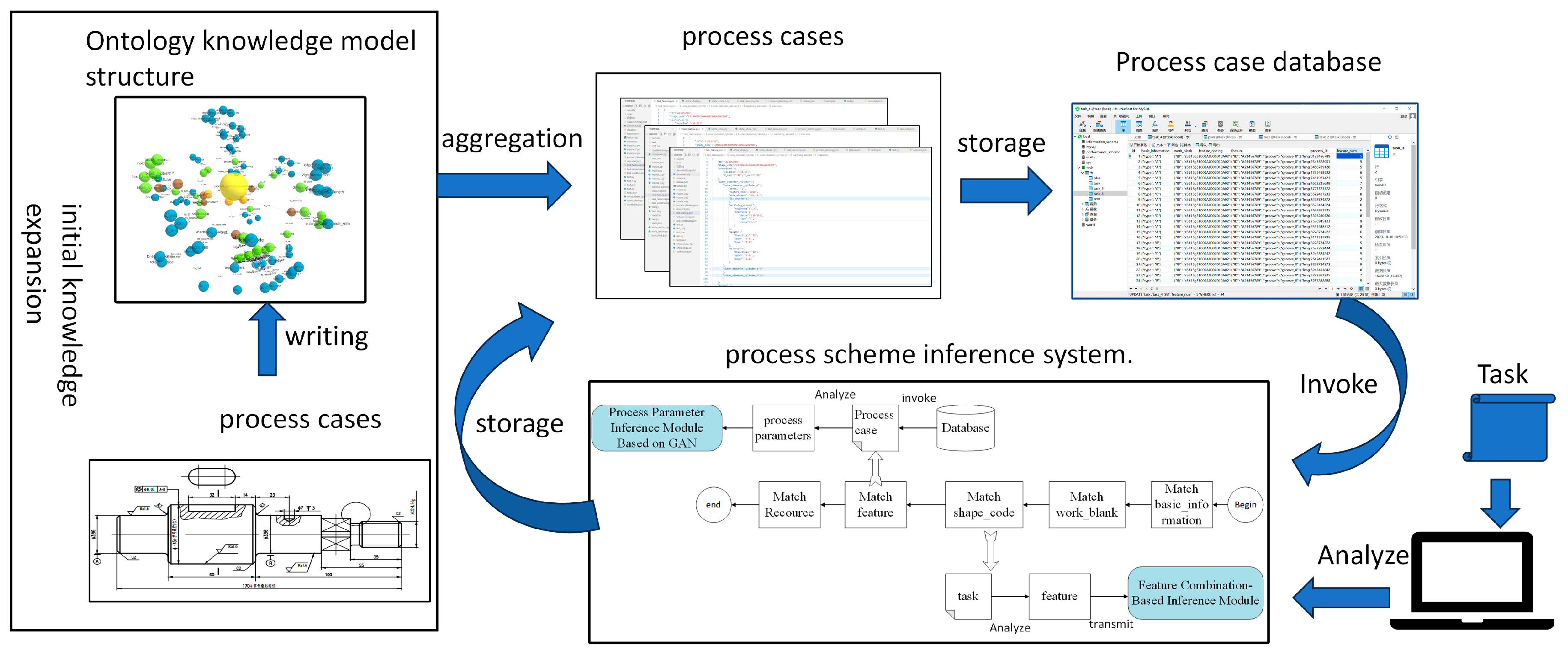
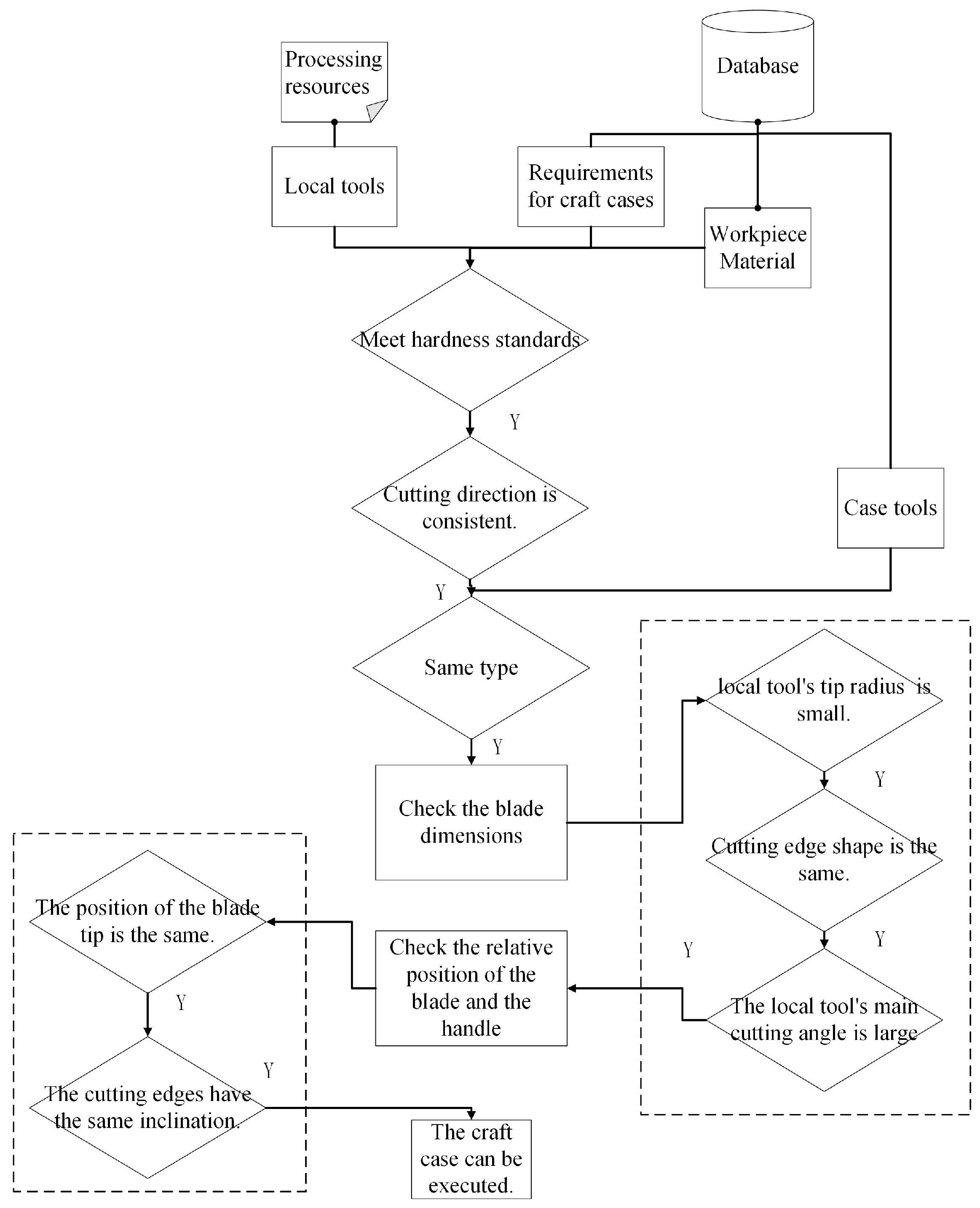
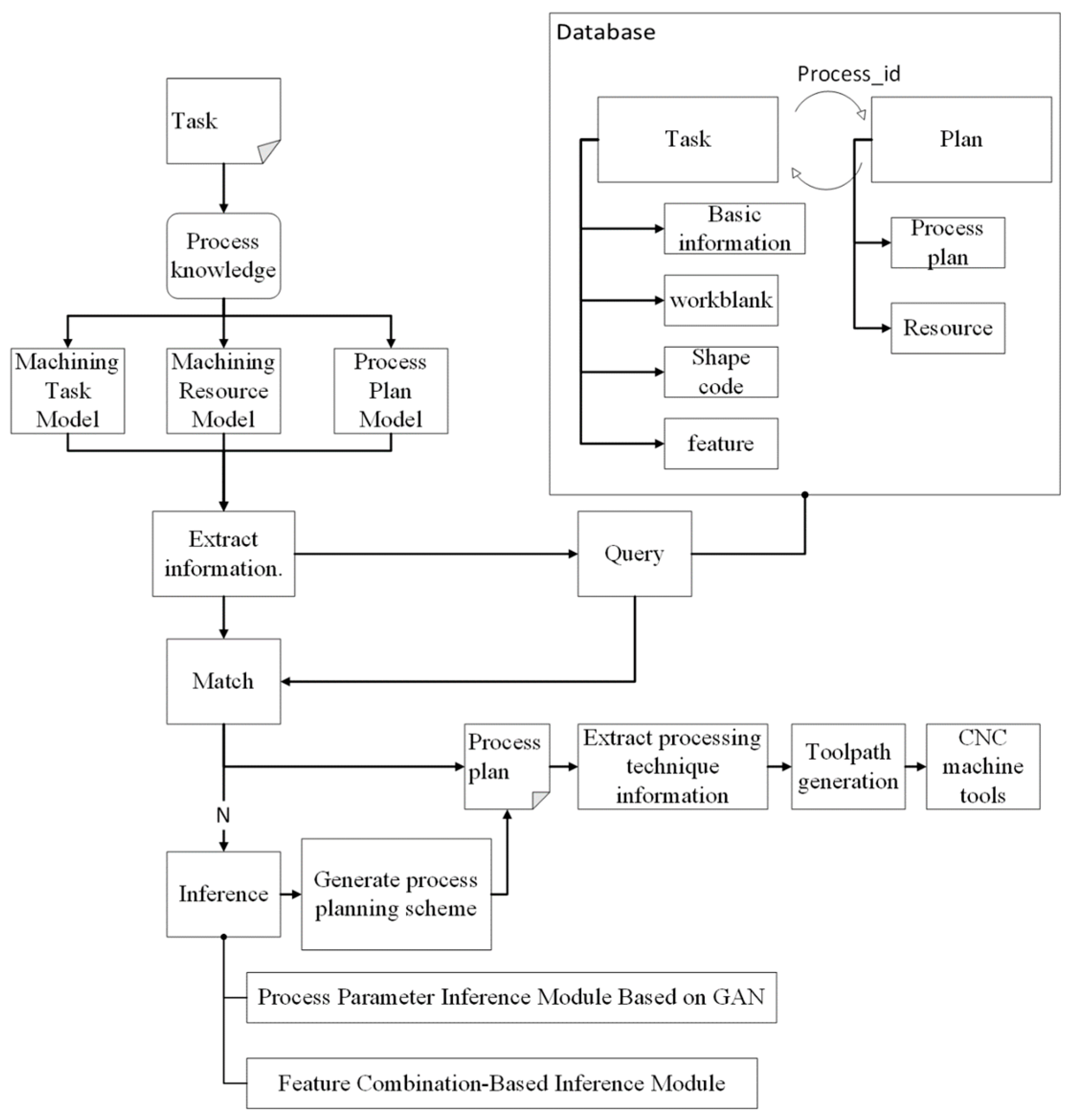
The design of the process knowledge database accomplishes more than just large-scale storage and management of manufacturing process knowledge; it establishes a dynamically updatable knowledge ecosystem that forms the foundation for subsequent process planning. In typical application scenarios, after users input machining task requirements and available resource information, the system employs intelligent retrieval mechanisms to match similar cases from the knowledge base and outputs process planning solution files (as demonstrated by the database matching module in Figure 8). However, real-world production environments present greater complexity, requiring the system to handle diverse operating conditions. To address this challenge, our solution adopts a modular design philosophy, implementing specialized reasoning modules (shown as the four branches in Figure 8) for different operational scenarios.

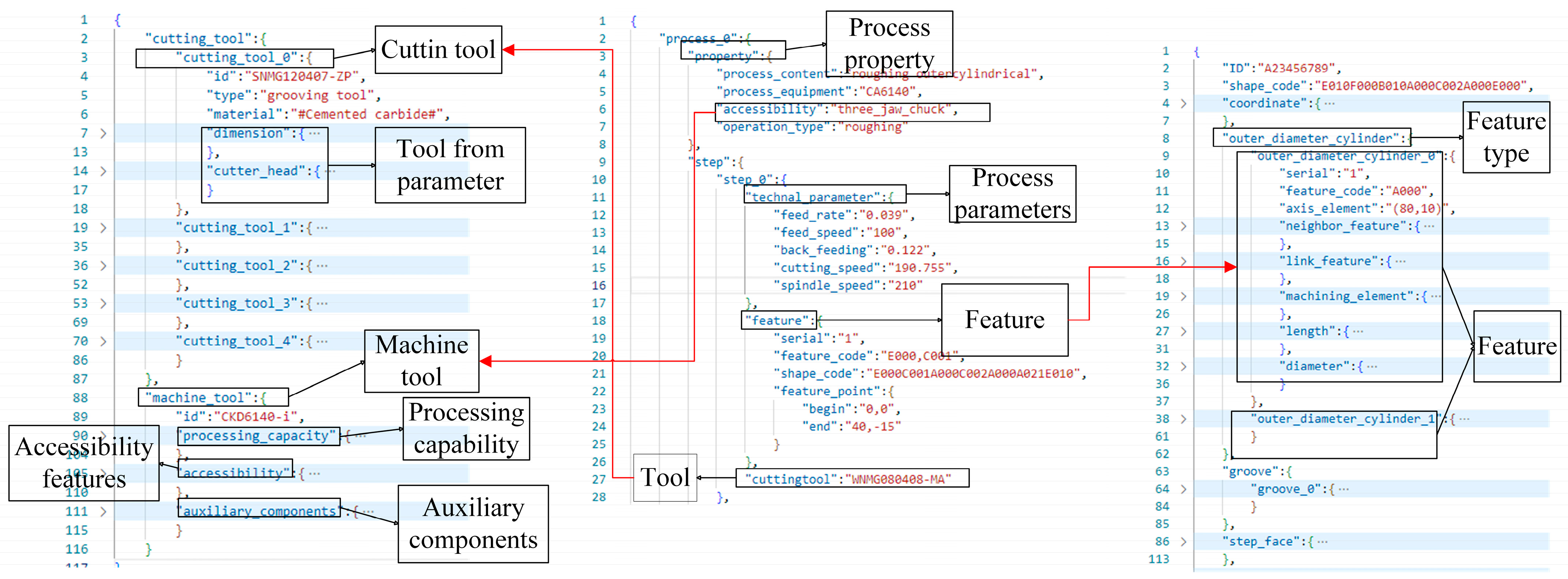
The matching module based on the database performs case screening from the process knowledge base following a hierarchical sequence: (1) blank information, (2) workpiece geometry, (3) feature attributes, and (4) machining resources, identifying cases that fully match the machining task requirements. When exact matching fails, the system retrieves the most similar case from the process database and adapts it through targeted modifications to generate a new process plan that complies with task specifications.

A failed shape code match indicates the absence of geometrically identical cases in the process knowledge database. The system consequently transitions to the ‘feature-combination-based reasoning module’, bypassing the ‘feature similarity assessment’ matching phase entirely.

This study utilizes the nearest-neighbor indexing method for case matching, based on the similarity calculations between instances, which include local similarity and global similarity. Global similarity refers to the similarity of individual features, while local similarity characterizes the degree of similarity of a specific attribute within a feature, serving as the foundation for calculating global similarity. Global similarity quantifies the level of similarity between feature instances, derived from the weighted sum of the local similarities.

3.1.1. Weighted Similarity Calculation Method Based on Euclidean Distance

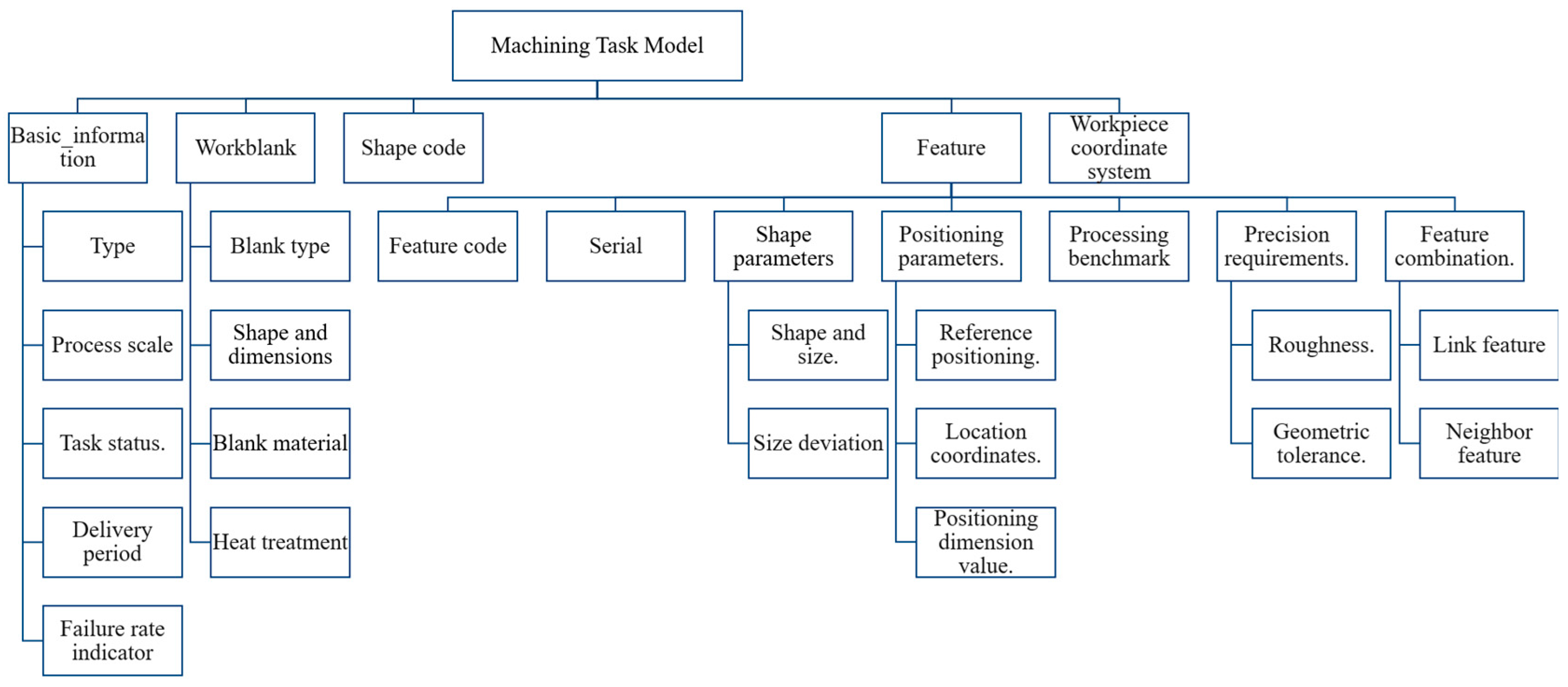
Matching feature attribute information involves checking all machining requirements within the machining task, including the dimensions, dimensional tolerances, geometric tolerances, and roughness of each feature, to ensure that the machining plan fully complies with the requirements of the machining task.

Firstly, the similarity calculation in task matching is based on numerical distance comparisons rather than statistical data or vector distance comparisons. Therefore, this study chooses to use Euclidean distance (straight-line distance) for the similarity calculation. The formula for Euclidean distance is shown in Equation (1), where $x_i$ and $y_i$ represent the numerical values for the machining task and the process case when calculating the same dimension.

$$E_d(x, y)={\displaystyle \frac{1}{1+\sqrt{{\sum }_{i=1}^k{\left(x_i-y_i\right)}^2}}}$$

(5)

In addition, attention must also be paid to whether the positioning references, types of errors, and dimensions are the same during the actual matching process. The following formula is used for this judgment:

$$i_n(x,y)=\left\{\begin{array}{c}1(x=y)\\ 0(x\ne y)\end{array}\right.$$

(6)

From the definitions provided earlier, it can be seen that the attributes of a feature consist of size information, precision requirements, surface quality, positional information, and so on. The formula for calculating the local similarity of each component attribute can be expressed as follows:

$${sim}_{Ra}=E_d\left({\displaystyle \frac{R_t}{R_t+R_p}},{\displaystyle \frac{R_p}{R_t+R_p}}\right)$$

(7)

$${sim}_g={\displaystyle \frac{1}{n}}\sum _{i=1}^n\left[i_{datum}{i}_{type}{E}_d\left({\displaystyle \frac{v_t}{v_t+v_p}},{\displaystyle \frac{v_p}{v_t+v_p}}\right)\right]$$

(8)

$${sim}_p={\displaystyle \frac{1}{n}}\sum _{i=1}^n{E}_d\left({\displaystyle \frac{{\mathrm{T}}_t}{{\mathrm{T}}_t+{\mathrm{T}}_p}},{\displaystyle \frac{{\mathrm{T}}_p}{{\mathrm{T}}_t+{\mathrm{T}}_p}}\right)$$

(9)

where ${sim}_{Ra}$, ${sim}_g$, ${sim}_p$ represent the similarity of surface quality, geometric tolerance, and dimensional tolerance, respectively. In Equation (7), R denotes roughness. The subscript t indicates information within the machining task, while the subscript p pertains to information within the process case, and the same applies below. In Equation (8), $i_{datum}$ signifies the assessment of the datum, $i_{type}$ indicates the judgment of whether the type of geometric tolerance is the same, and v represents the tolerance value. In Equation (9), T indicates the tolerance grade of dimensions. For the basic dimensions of features, due to the varying types of features and differing compositions of dimensions, the similarity calculation formulas for basic dimensions differ, as detailed in

Table 5. The formula for calculating the similarity of basic dimensions with different features.

Feature	Formula for Calculating Similarity	Comment
Outercylindrical	${sim}_d={\displaystyle \frac{1}{2}}\left[E_d\left(d_t,d_p\right)+E_d\left(l_t,l_p\right)\right]$	d is the outer diameter, and l is the outer length.
Cone	${sim}_d={\displaystyle \frac{1}{2}}\left[E_d\left(D_t,D_p\right)+E_d\left(d_t,d_p\right)+E_d\left(l_t,l_p\right)\right]$	D is the maximum diameter, d is the minimum diameter, and l is the length in the axial direction.
Groove	$$\begin{gathered} {sim}_d={\displaystyle \frac{1}{4}}{i}_{type}\left[E_d\left(d_t,d_p\right)+E_d\left(l_t,l_p\right)+E_d\left(p_t,p_p\right) \\ \hspace{1em}\hspace{1em}\hspace{1em}\hspace{1em}\hspace{1em}\hspace{1em}+E_d\left(c_t,c_p\right)\right] \end{gathered}$$	$i_{type}$ is used to determine the type. key: d is the width, l is the length, p is the depth, and c is the positioning distance; groove: l is the length of the groove on the Z-axis, d is the length of the groove bottom, p is the depth, and c defaults to 0.
Circle	${sim}_d={\displaystyle \frac{1}{2}}{i}_{type}\left[E_d\left(d_t,d_p\right)+E_d\left(c_t,c_p\right)\right]$	$i_{type}$ is used to determine the type, d is the diameter of the arc, and c is the positioning distance of the center
Roundface	$$\begin{gathered} {sim}_d={\displaystyle \frac{1}{3}}{i}_{type}\left[E_d\left(d_t,d_p\right)+E_d\left(p_t,p_p\right) \\ \hspace{1em}\hspace{1em}\hspace{1em}\hspace{1em}\hspace{1em}\hspace{1em}+E_d\left(c_t,c_p\right)\right] \end{gathered}$$	$i_{type}$ is used to determine the type, d is the diameter of the hole, and p is the depth of the hole, c is the positioning distance of the center
Screwthread	$$\begin{gathered} {sim}_d={\displaystyle \frac{1}{3}}{i}_{type}{i}_{Direction}\left[E_d\left(d_t,d_p\right)+E_d\left(p_t,p_p\right) \\ \hspace{1em}\hspace{1em}\hspace{1em}\hspace{1em}\hspace{1em}\hspace{1em}+E_d\left(c_t,c_p\right)+E_d\left(P_t,P_p\right) \\ \hspace{1em}\hspace{1em}\hspace{1em}\hspace{1em}\hspace{1em}\hspace{1em}+E_d\left(n_t,n_p\right)\right] \end{gathered}$$	$i_{type}$ represents the thread profile identification, $i_{Direction}$ indicates the thread direction assessment, d is the diameter, p stands for depth, c is the positioning distance, P is the pitch, and n represents the number of threads.
Taperscrewthread	$$\begin{gathered} {sim}_d={\displaystyle \frac{1}{3}}{i}_{type}{i}_{Direction}\left[E_d\left(d_t,d_p\right)+E_d\left(P_t,P_p\right) \\ \hspace{1em}\hspace{1em}\hspace{1em}\hspace{1em}\hspace{1em}\hspace{1em}+E_d\left(n_t,n_p\right)\right] \end{gathered}$$	$i_{type}$ represents the thread profile identification, $i_{Direction}$ indicates the thread direction assessment, d is the diameter, P is the pitch, and n represents the number of threads.

below.

Based on the analysis above, we can derive the formula for calculating the overall similarity of features as follows:

$${sim}_f=i_d\left(s_t,s_p\right)·(w_1{sim}_{Ra}+w_2{sim}_g+w_3{sim}_d+w_4{sim}_p)$$

(10)

where $s_t$, $s_p$ represent the feature serial numbers in the machining task and process case, respectively, used to distinguish different individuals within the same category of features; $w_1$~$w_4$ are the weight coefficients.

3.1.2. Determine the Weight Coefficients

This study employs subjective assignment and determines the specific weight values through objective statistical analysis. First, based on domain-specific research and empirical knowledge, we conduct preliminary subjective assignments of parameters by considering the priority levels and interrelationships of various local attributes. Subsequently, statistical analysis methods are employed to screen and validate the optimal weight combination, ensuring both objectivity and scientific rigor in weight determination. The specific method is as follows:

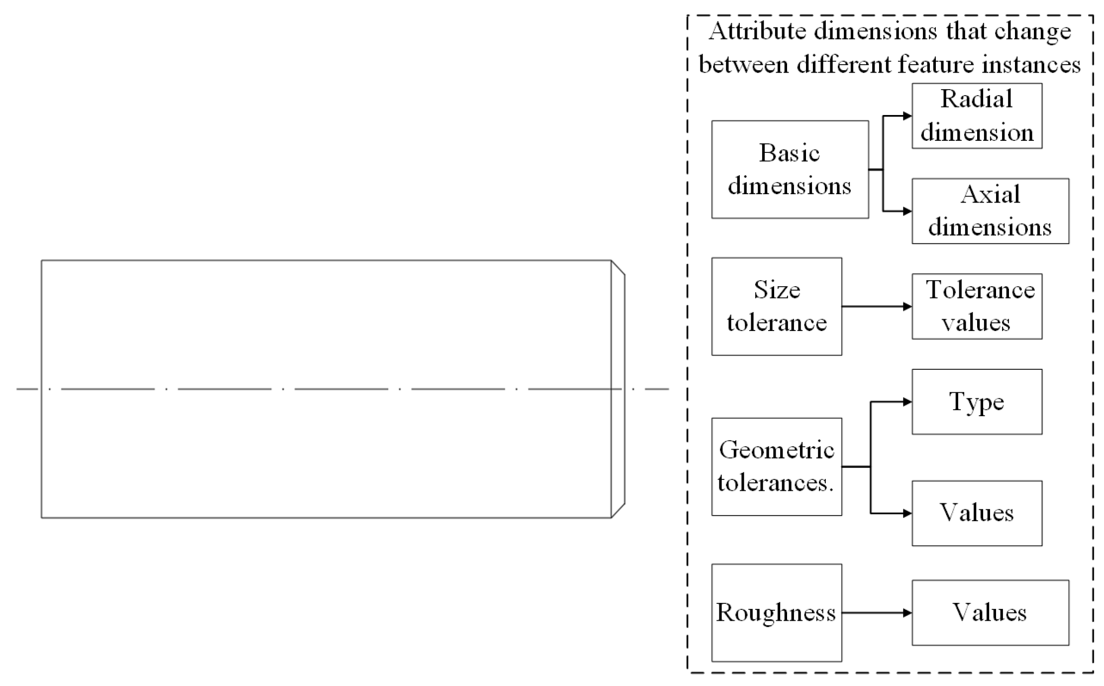
(1) Taking the external circular feature as an example, based on the knowledge modeling of external circular features discussed above, 51 groups of external circular feature instances with differing attribute information were randomly generated and stored in the database. As shown in Figure 9, these instances vary randomly across six dimensions, resulting in different external circular feature instances.

(2) The setting of weights satisfies the following two conditions: $\sum w_i=1$, $w_i\ge 0$. By reviewing the relevant literature [23,24,25], it was found that the basic dimensions of features have the greatest impact on the determination of similar cases, while the other three attributes have a smaller influence. Based on this observation, five sets of weight parameters have been established, as shown in

Table 6. Weight parameter settings.

Serial	$\mathbf{Surface} \mathbf{Quality} {\mathit{w}}_1$	$\mathbf{Geometric} \mathbf{Tolerance}{\mathit{w}}_2$	$\mathbf{Basic} \mathbf{Dimensions} {\mathit{w}}_3$	$\mathbf{Dimensional} \mathbf{Tolerance} {\mathit{w}}_4$
1	0.05	0.05	0.8	0.1
2	0.1	0.1	0.7	0.1
3	0.1	0.1	0.6	0.2
4	0.15	0.15	0.5	0.2

.

(3) Randomly select an external circular instance from the database as the target feature. Based on the weight groups set in Table 6 calculate and determine the top 10 similar feature instances for each weight group. A threshold ε is established to assess attribute reusability; when the local similarity is greater than or equal to ε, the attribute can be reused. If there are reusable parts in the feature attributes of a single feature instance, mark the attribute as 1; otherwise, mark it as 0. Use $S_1$, $S_0$ to record the counts of marked 1 s and 0 s, respectively. Finally, compile the results S for each weight combination and select the weight group with the highest S value.

$$S={\displaystyle \frac{S_1}{S_1+S_0}}$$

(11)

where $S_1$ is the number of attributes marked as 1 among the top 10 feature instances, and $S_0$ is the number of attributes marked as 0 among the top 10 feature instances. The weight combination that yields the maximum value of the evaluation criterion S is designated as the weight setting for Equation (11).

In process case similarity assessment, there is a theoretical positive correlation between the similarity value (Sim_f) and the reusable part of the case (S_1), i.e., a higher similarity value usually corresponds to a larger reusable content. However, due to the variability in feature weight assignment, there may be a mismatch between the two: when the similarity contribution of some high-weighted features is large, the overall similarity value may still be high, even though the actual reusable portion is small. This anomaly provides an important basis for the reasonableness test of the weight setting, specifically. Firstly, the S value should have a positive relationship with the Sim_f value. Secondly, the cases with a larger similarity value should also have a larger corresponding S value.

(4) Firstly, the threshold ε is determined, and a random set of weight coefficients is selected to calculate the similarity and evaluation criterion S, with the results shown in Figure 10. It can be observed that when the threshold ε is set below 0.95, the majority ${sim}_{Ra}$, ${sim}_g$, ${sim}_p$, ${sim}_d$ represent reusable components, and the distinction between cases is relatively small. However, when the threshold ε is set above 0.95, there are instances of high similarity values, but the reusable component ($S_1$) becomes 0. Therefore, the threshold is set at ε = 0.95.

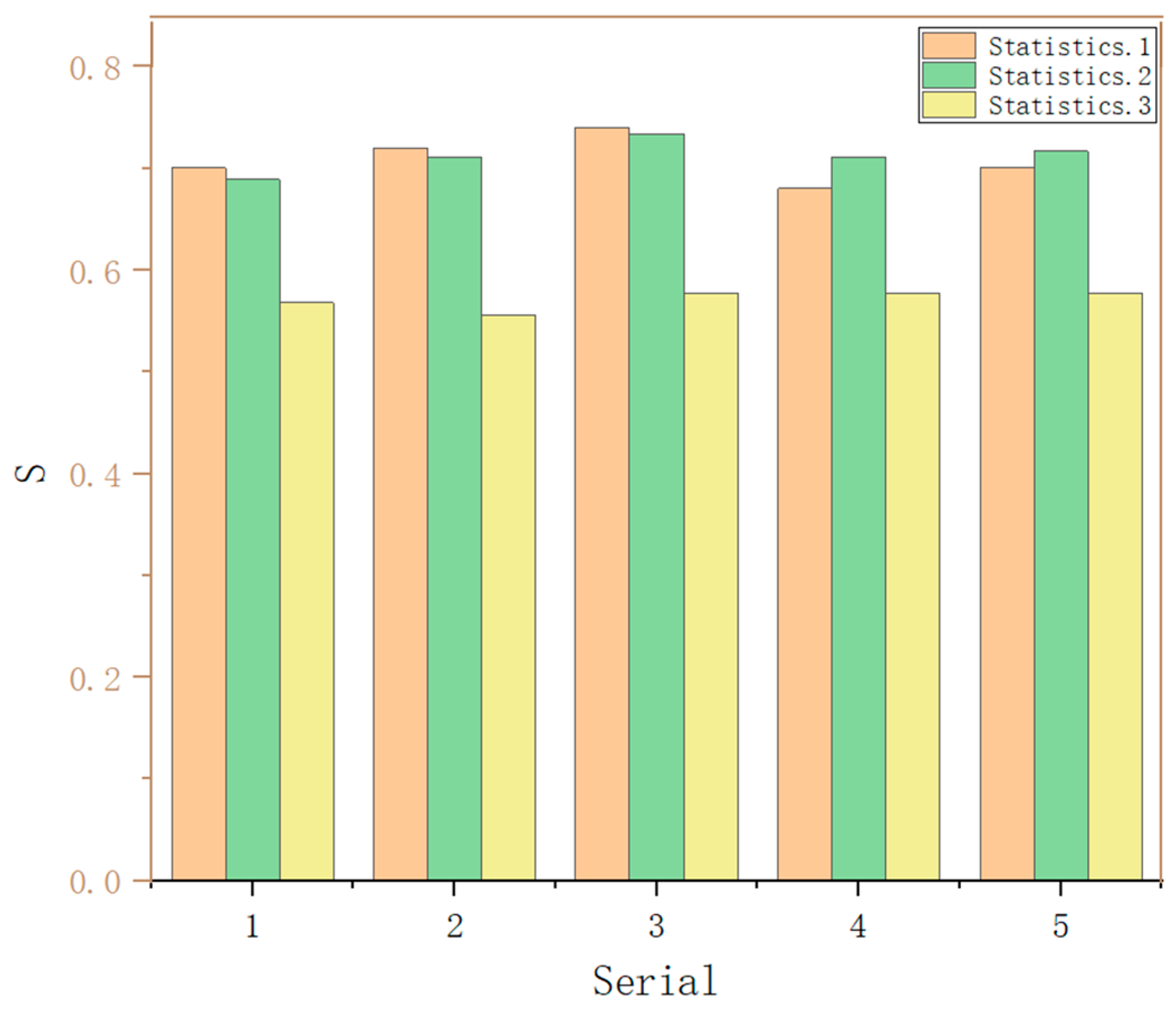
In order to ensure the reliability of the statistics, steps (1), (2), and (3) are repeated three times, with the target instance and target features randomly selected each time. The final summarized results are shown in Figure 11. It can be observed that the S value of the third weight group is significantly higher than that of the other weight groups, with evaluation criterion S values of 0.74, 0.825, and 0.65, respectively. Therefore, the third set of weight coefficients is chosen, $w_1=0.1, w_2=0.1, w_3=0.6, w_4=0.2$.

The feature similarity ${sim}_f$ in the above equation is used to calculate the similarity of individual features. Considering the differences in feature types and the potential issue of non-uniqueness among similar features, the feature matching module is divided into multiple sub-modules, and each sub-module inspects a specific type of feature. The sub-module differentiates between different individual features within the same category based on keyword feature encoding and feature indices, like part $i_d\left(s_t,s_p\right)$ in Equation (10).

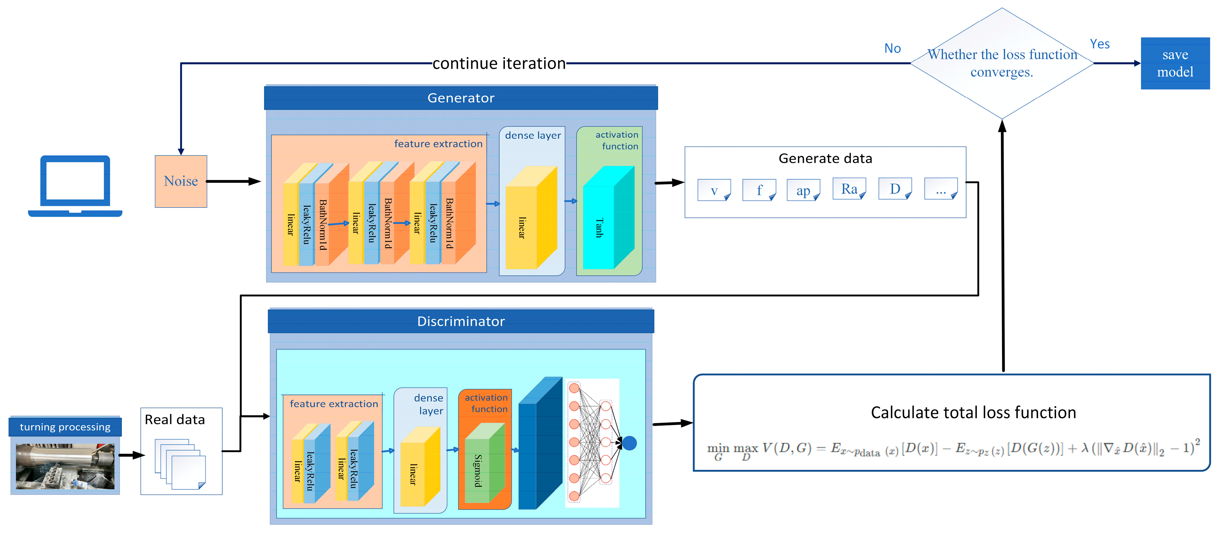
When no process cases can be found that meet the similarity requirements, the matching module does not produce an output, and the system transitions to Process Parameter Inference Module Based on GAN.

3.1.3. Processing Resource Inspection

In the database, if there are cases that meet the similarity matching requirements, a further inspection of the processing resources is needed to verify whether the processing site can execute the process case. During the verification process, the first step is to check whether the machine model and tool codes can match corresponding mappings in the local resources. If the relevant mapping characters cannot be found, it indicates that the actual resources differ from those used in the case, necessitating a further examination of whether the processing capabilities of the local machines or tools can support the execution of the proposed solution.

The inspection of the tool resource replacement rule process is shown in Figure 12. First, the analysis of the tool and workpiece material yields criteria for the rational selection of tool materials commonly used in high-speed cutting (see

Table 7. Rational selection criteria for common tool materials in high-speed cutting.

Workpiece Material	Tool Material	Application Conditions
aluminum alloy	ultra-fine grain carbide, PCD	cutting speed: 2000~4000 m/min feed rate:3~12 m/min
cast aluminum alloy	Si3N4-based ceramic tool	cast aluminum alloy with Si content less than 12%
	PCD, CVD diamond-coated tool	Si: 12%~18%
	PCD, CVD diamond-coated tool	Si: 16%~18%
cast iron	coated carbide, cermet	cutting speed: 350~750 m/min
	Si3N4-based ceramic tool	510~2000 m/min
	CBN	2000~4500 m/min
	CBN is not recommended for this application; instead, ceramic tools	The workpiece consists predominantly of ferrite
carbon steel	coated carbide, cermet, CBN	cutting speed: 500~800 m/min
high-hardness steel (HRC > 45)	cermet, TiC-coated carbide, CBN	cutting speed: 150~180 m/min

for details). According to the workpiece material, the reference table can determine the most suitable type of tool material. The local tool’s material is then checked to verify whether it meets the machining conditions.

3.2. Process Parameter Inference Module Based on GAN

3.2.1. Generation of Process Parameters Based on GAN

For situations where there are entries in the database with the same processing task feature coding but do not match in similarity calculations, a reasoning model based on GAN is proposed. This module utilizes information, such as feature dimensions, surface quality, tool, and workpiece materials, to generate an optimal combination of cutting parameters that meet specific conditions through the GAN. Ultimately, based on the process route and machining sequence, a process plan that meets the requirements of the processing task is formulated by adjusting the steps of the approximate plan and replacing process parameters while ensuring the surface roughness.

The GAN mainly consists of two components: the generator and the discriminator. The primary function of the generator is to capture the distribution of samples and adjust its weights based on feedback from the discriminator model regarding the generated results. This process aims to maximize the closeness between the distribution of generated process parameters and the true distribution of the process parameters. The main function of the discriminator is to engage in adversarial learning with the generator, continuously improving its accuracy in distinguishing between real and fake data. This, in turn, encourages the generator to produce more realistic processing data. The specific network model is illustrated in Figure 13.

As the model continues to be trained, the generated data from the generator become increasingly similar to the real processing data until the generator can produce parameters that closely resemble the true data. Once the model training is complete, samples are drawn from a normal distribution and input into the generator, which outputs the process parameters. The generated output includes eight parameters: feature coding F, machining allowance for finishing Z, tool D, dimensional accuracy C, cutting speed v, depth of cut ap, feed rate f, and roughness Ra. During usage, the required cutting parameters can be determined based on conditions such as surface roughness, dimensional accuracy, and the tool.

3.2.2. Adjustment of Process Parameters Based on Similar Case Studies

After obtaining a trained GAN model, it is necessary to consider how to utilize the generated cutting parameters to create a process plan that meets the machining requirements. The specific operational flow is illustrated in Figure 14. First, the overall similarity score is used to identify the most similar case (problem_plan). Then, based on this case, the cutting parameters are adjusted to generate a new plan. During this process, the features from the most similar case that do not meet the required similarity criteria are referred to as problem features (problem_feature).

The specific steps are as follows: First, read the intermediate information table output from the matching module to obtain information on problem features, feature attributes, and similarity scores. The plan with the highest similarity value is selected as the most similar case, and the relevant machining operations for the identified problem features are recorded for subsequent processing. Meanwhile, the extracted problem feature attributes and other information are passed to the trained GAN generator to generate the corresponding cutting parameters. Finally, the generated process parameters are applied to the most similar case according to the plan adjustment strategy. The plan adjustment strategy specifically refers to the following:

(1) Adjustment methods for steps with different feature sizes.

When machining shaft-type components, if the characteristic dimensions of the machining task differ from those in the process case, the adjustments can be categorized into two situations: axial dimensions and radial dimensions. For differences in axial dimensions, it is sufficient to adjust the feature coordinate points in the process plan. For differences in radial dimensions, the overall cutting depth must be adjusted according to the specific dimensions. This can be achieved during rough machining by either adding or removing process steps, adjusting the number of feed passes within steps, or modifying cutting depths, all to better adapt to machining task requirements.

(2) Adjustment methods for steps with different requirements for roughness or precision levels.

In cases where the roughness or accuracy-level requirements of the most similar cases differ from those of the machining task, it is necessary to adjust the cutting parameters of the final machining step for that feature in the prototype case. This adjustment essentially involves replacing the original data with the cutting parameters generated by the GAN generator. Since the cutting depth in the generated parameters may differ from the original data, a direct replacement could lead to changes in the total cutting depth, which, in turn, would cause changes in the basic dimensions. The adjustment rules are shown in

Table 8. Rules for adjusting process parameters when processing requirements differ.

Machining Allowance	Corresponding Operations
$Z_g=Z_{\mathrm{p}}$	1. The last operation step of this feature replace parameter.
$Z_g>Z_{\mathrm{p}}$	1. The initial step of this feature processing chain changes the cutting depth, $a_p=a_{p0}-(Z_g-Z_p)$ 2. The last operation step of this feature replace parameter.
$Z_g<Z_{\mathrm{p}}$	1. The initial step of this feature processing chain changes the cutting depth, $a_p=a_{p0}+(Z_{\mathrm{p}}-Z_g)$ 2. The last operation step of this feature replace parameter.

.

$Z_g,Z_{\mathrm{p}}$ represent the machining allowances reserved in the generator for generated parameters and the machining allowances in the prototype case before the forming step, respectively. The value of $Z_{gan}$ corresponds to the $a_p$ value in the parameters generated by the generator; $a_{p0}$ denotes the original cutting depth for that step.

Taking the outer circle feature as an example, as shown in Figure 15, the grid line section represents the cutting depth $Z_p$ from the last machining step in the most similar case; the dashed section on the right indicates the cutting depth $Z_g$ generated by the GAN model based on the roughness requirements of the machining task. If $Z_p$ is directly replaced with $Z_g$ while the blank size remains unchanged, it will result in a smaller amount of material being removed, causing the outer diameter $D_{case}$ to increase. To meet the dimensional requirements of the machined part, the machining allowance of the previous step must be adjusted after replacing the cutting depth parameters, with the additional cutting depth being $Z_p-Z_g$. Subsequently, a step check is conducted on the new plan to ensure it complies with general machining rules. Finally, the process planning scheme is instantiated and output to complete the inference process.

3.3. Feature Combination-Based Inference Module

3.3.1. Determine the Processing Chain Based on Feature Information

When the process knowledge database lacks cases matching the feature codes of the machining task, the system first decomposes the task into individual feature machining operations. It then retrieves corresponding feature machining chains from the database based on feature information and finally reorganizes the machining chain steps according to predefined rules to generate a new process plan. The detailed workflow is illustrated in Figure 16.

First, the machining task is decomposed using keywords such as feature_code and serial to convert the description into a single feature. Next, similar feature cases that meet the machining requirements are matched in the database based on the similarity of the feature machining chain (${sim}_{f2}$). The feature processing chain refers to the entire machining process of a feature from the raw blank to completion. This process is repeated until all task features are retrieved.

Finally, the processing operations at different stages of the machining chain are marked according to the associated feature type reference table (Table 8). For simple_feature, the machining chain file is recorded directly; for complex_feature, the machining chain is divided into two parts based on the processes: machining of simple_feature and forming of complex_feature.

The calculation formula for the similarity of the feature processing chain (${sim}_{f2}$) of this module is as follows:

$${sim}_{f2}=w_5(w_1{sim}_{Ra}+w_2{sim}_g+w_3{sim}_d+w_4{sim}_p)+w_6{i}_{feature}\left(F_t,F_p\right)$$

(12)

In the equation, $(w_1{sim}_{Ra}+w_2{sim}_g+w_3{sim}_d+w_4{sim}_p)$ is the content of the feature similarity ${sim}_f$, defined by the same Equation (10). F refers to the neighboring features (neighbor_feature), and $i_{feature}\left(F_t,F_p\right)$ is used to determine whether the types of the neighboring features are the same. To maintain the similarity value at a maximum of 1, coefficients $w_5$ and $w_6$ are introduced, where it must satisfy the conditions $w_5<1$, $0<w_6<1$, $w_5+w_6=1$. Since adjacent features can directly affect the subsequent reorganization of the machining chain, to better assess the impact of adjacent features, it was found that when the coefficient $w_6=0.5$ and the adjacent features are different, the similarity value of the feature processing chain ${sim}_{f2}$ will always be less than or equal to 0.5. Therefore, it is determined that $w_6=0.5$, which corresponds to $w_5=0.5$.

If the filtered feature similarity ${sim}_{f2}$ does not have any case features equal to 1, but there are cases that are less than 1 and greater than 0.5, then the GAN parameter generator (Section 3.2) will be invoked to replace the original cutting parameters and obtain new machining chain information. Further details on this process are not elaborated here.

3.3.2. Feature Combination and Reorganization Process Route

The feature-based reconfiguration of the process route effectively constrains the overall process flow through the arrangement of operations, using process rules to regulate the specific steps involved. This results in a set of process steps arranged in a defined order, known as the process planning scheme.

This study proposes a method for reconfiguring process routes based on the definition of associated features (Section 2.2). The reconfiguration of the overall process plan for the workpiece is mainly divided into two parts: the reconfiguration of process routes for simple features and the completion of processes for complex features, as shown in Figure 17. The rules for the reorganization of process steps refer to various process constraints, which can be categorized into mandatory constraints and optimization constraints, as illustrated in

Table 9. Process route sorting constraints.

Constraint Type	Constraint	Comment
Mandatory constraints	Positioning Constraints	Features that serve as a priority for positioning.
	Reference Constraints	In dimensional tolerancing, the features serving as references should be prioritized in processing.
	Clamping Constraints	Clamping that does not affect other features.
	Non-destructive Constraints	Subsequent processing must not damage the existing processing.
	Primary and Secondary Constraints	Prioritize processing of key features.
Optimization constraint	Clamping Frequency Constraints	Use as few clamping instances as possible.
	Tool Change Frequency Constraints	Use as few tool changes as possible.
	Clustering Constraints	Try to complete the machining in one setup.

. In theory, it is not possible to satisfy all constraint conditions to achieve the sorting of the processing route. However, if the final process planning scheme meets the constraints of a mandatory and priority nature, it can be considered a reasonable process planning scheme.

Since the simple_feature only includes external circular cylinders, cones, and end face features, their basic sequence of operations is fixed: facing—rough turning—semi-fine turning—fine turning, with any additional processes inserted in order. The process sequence for complex_features needs to be sorted according to processing rules. For instance, if a workpiece has a tool retreat groove, threaded features, and a keyway feature, the processing of the keyway requires a machine tool change, which can affect processing efficiency and precision. Additionally, the impact of processing scale and precision must be considered. If the processing scale is small and there are requirements on the precision of the keyway position, the keyway processing can be scheduled before the threading operation, whereas if the processing scale is large and the position of the threaded features has little impact on clamping, the keyway can be processed after the threading.

The operations for the reconfiguration of process steps in both parts are fundamentally similar: First, the steps are categorized based on information, such as tools, processing equipment, and feed direction. Then, the steps within each category are sorted according to feature positions and process parameters. The sorting rules adhere to process constraints such as prioritizing primary features over secondary ones and referencing features before others.

Taking the workpiece shown in Figure 18 as an example, this section details the working principle of the machining chain reorganization module. The system first automatically generates machining chain data for partial features based on the workpiece’s characteristic information, with some representative data shown in

Table 10. Machining chain information for some features in a shaft.

Feature	Step	Machine	Cutting Tools	Link Feature	Processing Direction	Datum
O1	1-1	01	01, 02, 03	0	1	O5
	1-2	01	01, 02, 03	0	1
	2-1	01	01, 02, 03	0	1
	3-1	01	01, 02, 03	0	1
	3-2	01	01, 02, 03	0	1
	4-1	03	01, 02, 03	0	1	O4
O6	1-1	01	01, 02, 03	0	−1
	1-2	01	01, 02, 03	0	−1
	2-1	01	01, 02, 03	0	−1
	3-1	01	01, 02, 03	0	−1
	3-2	01	01, 02, 03	0	−1
G1	1-1	01	02	0	1
	2-1	01	04	1-O1	1
G3	1-1	01	02	0	−1
	2-1	01	04	1-O1	−1
F1	1-1	01	01, 02, 03	0	−1
	2-1	01	02	1-O3	−1
	3-1	01	05	1-O3	−1	O4
	4-1	--
K1	1-1	01	01, 02, 03	0	−1
	2-1	02	06	1-O5	−1	O3

. In the machining chain information table, the ‘step’ field uses a hierarchical coding system of ‘process number-step number’ (e.g., ‘1-1’ indicates the first machining operation in Process 1). The ‘link feature’ field employs a feature classification coding mechanism: Code ‘0’ denotes machining steps belonging to main category features. Code ‘1-A3’ indicates a subcategory feature whose associated main category feature is external cylinder O3.

During process planning, for simple features (subcategory features) with relatively fixed operation sequences, optimization focuses primarily on step reorganization. Taking groove G1 machining as an example, Step 1-1 is completed using Tool #02. To improve machining efficiency, operations with the same machining direction and equivalent process level (e.g., Steps 1-1 and 1-2 for external cylinder O1) also utilize Tool #02, thereby optimizing tool resource allocation and reducing tool change frequency.

After establishing the process route for simple features, priority shifts to optimizing the machining sequence for complex features (main category features). Taking threaded feature F1 as an example, since its datum surface is external cylinder O2, the machining of O2 (Operation 3-1) must precede thread machining according to the principle of datum priority.

For determining the sequence among groove features G1 (Operation 2-1), G3 (Operation 2-1) and thread F1 (Operation 3-1), the following constraints must be comprehensively considered: Tool change constraint: different tools are required for G1/G3 vs. thread F1 machining. Fixturing constraint: separate fixturing is needed for G1 and G3. Equipment constraint: rough grinding of external cylinder O1 (Operation 4-1) must be completed on dedicated machine tool #03. Through this constraint analysis, the optimized process route is determined as G3→G1→F1→O1 (4-1).

The final process scheme obtained by the system is shown in Figure 19, with the following workflow: facing → rough turning → semi-finish turning → finish turning → keyway milling → relief groove turning → thread turning → quenching and tempering → rough grinding.

4. Results

4.1. The Construction of the System

The construction of an intelligent process planning system based on a knowledge base mainly includes two parts: the construction of the knowledge base and the development of an intelligent decision-making model for processing techniques. The overall system architecture is shown in Figure 20. The knowledge base is developed using SQL language on the Navicat15 for MySQL 15.0.19 software platform, while the intelligent decision-making model for processing techniques is developed in Python 3.7.15 on the Visual Studio 1.98.2 platform.

4.2. Intelligent Generation and Validation of Process Parameters

4.2.1. GAN Generation Model Training

This study employs a faster and more stable WGAN-GP network structure as the core of the process parameter generation model. In the WGAN-GP model, the discriminator no longer simply performs a binary classification of real and fake data but acts as an evaluator, scoring the proximity of the data to reality. Real data receive a high score, while the data generated by the generator receive a lower score. The loss function of the discriminator consists of three parts: real data, generated data, and the Wasserstein distance. By optimizing the discriminator through backpropagation, its ability to distinguish between real and generated data is constantly enhanced. The generator updates its network parameters based on gradient feedback to make the distribution of generated data closer to that of real data, thereby maximizing the discriminator’s score and achieving adversarial learning. When the scores assigned by the discriminator to real and generated data converge, it indicates that the generator has successfully captured the distribution characteristics of the real data, marking the completion of the training process.

This study utilizes carbide cutting tools to machine 40CrNiMoA alloy steel in order to verify whether the data generated by the intelligent process parameter generation model meet processing requirements in practical applications. The selected tool model is SNMG120408-ZP, with a tool holder model of MSBNR2525M12, the model CDE6140A, and a roughness measurement instrument, the TR240 high-precision surface roughness tester. The specific attribute parameters of the tool are provided in

Table 11. Cutting tool parameters.

Cutting Tool	Blade Tip Radius	Cutting Tool Edge Radius	Front Angle	Rear Angle	Main Deviation Angle
SNMG120408-ZP	0.8 mm	0.2 mm	10°	6°	75°

.

In this study, the cutting speed, feed rate, and cutting depth were varied across five levels, resulting in a total of 125 experimental groups. The variations in cutting speed were achieved primarily by changing the spindle speed. The training set of process parameters was preprocessed through standardization and data format conversion before being input into the network model for training. The training process utilized the Adam optimization algorithm, with the loss function set to binary cross-entropy loss (BCE loss). The model was optimized by minimizing the loss function to enhance its learning capability. The trend of the loss function over the training epochs is illustrated in Figure 21. The discriminator updated the model weights for optimization based on its error gradient through backpropagation, while the generator updated its weights in response to the gradient of the discriminator’s evaluation of the data. The two components are in an adversarial relationship during the training process, where a reduction in one party’s loss is accompanied by an increase in the other. When the model converges, the D_loss and G_loss stabilize. As shown, prior to 4000 steps, D_loss and G_loss fluctuate, while after 10,000 steps, both become relatively stable, with smaller fluctuations in loss, indicating that the model has essentially converged. The model has been saved, and the hyperparameters at this point have been recorded as follows: learning rate lr = 0.000015, batch size batch_size = 64, and gradient penalty coefficient gp = 10.

In order to better illustrate the performance of the model, this study additionally configured GAN and DCGAN as comparative network structures and introduced common GAN testing metrics, Inception Score (IS) and Frechet Inception Distance (FID), as evaluation criteria. In simple terms, both IS and FID are standards for evaluating generative networks, and their final results are scalar values. A larger IS value indicates better model performance, while a smaller FID value indicates better model performance. The configured network structure is shown in

Table 12. Relevant parameters of different network models.

Model	Optimizer	Lr	Batch	Epoch	Gen Layers	Dis Layers
GAN	Adam	0.001	64	200	3	2
DCGAN	Adam	0.0001	128	200	4	3
Process Parameter Generator	Adam	0.000015	64	200	4	3

:

All models were trained for 25,000 steps in the training set. After training is complete, the generator structures and their parameters for each model are saved. Finally, the generated data from each model are compared with the real data to calculate the evaluation metrics IS and FID. The evaluation results for each model are shown in

Table 13. Evaluation of the quality of generated data from different network models.

Model	IS	FID
GAN	3.620	30.20
DCGAN	6.453	53.64
Process Parameter Generator	7.140	29.84

:

It can be seen that, if FID is used as the standard, the FID values of the process parameter generator and GAN are significantly lower than that of the DCGAN, indicating that the process parameter generator and GAN, based on WGAN-GP, perform significantly better than the DCGAN model. Additionally, when using IS as the standard, the IS values of the process parameter generator and DCGAN are notably higher than that of GAN, indicating better performance. In summary, the process parameter generator based on WGAN-GP outperforms the conventional GAN model and the DCGAN model.

4.2.2. Verification of the Process Parameter Generation Model

Finally, the effectiveness of the process parameter generator is verified through actual processing. After the model training was completed, the computer sampled 1000 groups of original data from a normal distribution and passed them to the generator to output simulated process parameters and generate data for sampling. When the generated data fully matched the tool, feature coding, and other parameters in the training set, statistical analysis was conducted on the value ranges of the generated data compared to the training set data, as shown in

Table 14. Conformity of generated process parameters over the range of the training data distribution.

Parameter	Range of Real Data Values	Generate Data with a Reasonable Ratio
v	50–200	96.9%
ap	0.05–0.5	97.3%
f	0.035–0.159	95.5%
Total		93.6%

. It was determined that the generated data falling within the value ranges of the training set data were reasonable. The proportion of reasonable generated data for each parameter reached 93.6%.

To validate the effectiveness of the generated cutting parameters, a systematic experimental validation process was designed in this study. Parameter combinations with the same tool (D), feature code (F) and machining allowance (Z) were first screened from the generated data to ensure that the experiment focused on the correlation analysis of cutting amount (v, ap, f) and surface roughness (Ra). By randomly selecting 21 groups of generated parameters for the actual cutting test, the surface roughness data were obtained using the 5-point measurement method (5 cm interval), as shown in Figure 22, and the mean value of measured roughness (real_Ra) and its range of variation for each parameter combination were calculated. The quality assessment is based on the measured data, and the conditions for determining that the generated Ra value (GAN_Ra) is qualified are that it is both within the range of fluctuation in the measured value ([real_Ra_min, real_Ra_max]) and not lower than the measured mean value (≥real_Ra_mean). The comparison results are shown in Figure 23. Detailed data can be found in Appendix A.

GAN_Ra represents the surface roughness values generated by the generator, while real_Ra denotes the average roughness obtained from actual experiments under the same set of machining parameters. It was found that the proportion of generated data meeting the machining requirements reached 92%, indicating that the model is deemed to meet the usage requirements.

4.3. Functional Verification of the Intelligent Process Planning System Based on the Process Knowledge Database

To verify the feasibility of the model, relevant experiments were designed to validate the inference capabilities. Since the intelligent decision-making model for machining processes relies on the knowledge of process planning stored in the database, it is essential to ensure that the database contains a sufficient knowledge base. Therefore, two typical workpiece shapes were introduced, as shown in Figure 24. Without changing the feature combinations, random values for the dimensions, tolerance levels, surface quality, and other machining requirements for the features were generated using a calculator for adjustments. As a result, a total of approximately 500 sets of process cases were obtained.

After ensuring that a certain number of process cases are stored in the database, the structure is shown in Figure 25a. Information on certain features within the cases is illustrated in Figure 25b. The laboratory CNC machine tool used is CKD6140I, equipped with a Fanuc turning system. To rigorously demonstrate the advantages of our proposed knowledge-guided, GAN-enhanced hybrid multimodal reasoning method, we conduct systematic comparisons with traditional rule-based and case-based reasoning (RBR/CBR) approaches.

A machining task, as shown in Figure 26, along with the local tool information resources indicated in

Table 15. Cutting tool resources used in the experiment.

Serial	Blade Model	Blade Material	Magnetic Declination	Type
T01	WNMG080408-MA	Hard alloy M950	90°	External round cutting tool.
T02	SNMG120408-ZP	Hard alloyYBC152	90°	External round cutting tool.
T03	VBMT110302-FM	Quenched steel.CH65D	95°	External round cutting tool.
T04	16ERAG60-GX100	Tungsten steel	60°	Thread turning tool

, was submitted to the intelligent process planning system to test the inference capability of the reasoning model. Although the machining task does not resemble the planned case shape, all features present can be mapped to corresponding entries in the cases, ensuring the normal operation of the system’s reasoning mechanism.

The output results of the traditional case-based and rule-based reasoning system (Figure 27) exhibit evident disorganization and errors. This deficiency stems from exponential growth in rule combinations (‘rule explosion’) when multidimensional factors, including process parameters, equipment status, and environmental variables, interact, causing system latency and decision conflicts that compromise output accuracy.

The process plan generated by the proposed method is presented in Figure 28a, which visually demonstrates the solution’s characteristics and applicability, with logically arranged operations. After specifying the machine tool model and CNC system, the system further parses the process plan to produce detailed toolpaths, enabling physical workpiece fabrication, as shown in Figure 28b. Post-machining measurements of critical cylindrical surfaces revealed a roughness value of Ra 1.231 $\mathsf{\mu }\mathrm{m}$ (Figure 29), meeting specified requirements. All other dimensional tolerances were also satisfied, confirming the experimental workpiece fully complies with the designated machining task specifications.

5. Discussions

The experimental results demonstrate that the intelligent process planning system proposed in this study exhibits outstanding performance in both process parameter generation and process decision making.

In terms of process parameter generation, comparative experimental data with different generative network models confirm that the improved Generative Adversarial Network (GAN) adopted in this study outperforms traditional methods in key metrics, including parameter diversity, physical feasibility, and convergence speed. The generated process parameters not only satisfy theoretical constraints but also adapt to practical machining requirements. Through actual machining verification, the cutting parameters generated by this model (such as spindle speed and feed rate) can ensure machining quality, validating the usability of the generated data.

In terms of process decision making, the system outputs process programs for two typical machining tasks to meet the design requirements. The specific performance is as follows: (1) the allocation of machining resources is reasonable, realizing the optimal selection of cutting tools and machine tools; (2) the generated process parameters are scientific and effective, and the dimensional tolerance and surface roughness of the machined workpieces meet the preset standards; (3) the arrangement of process routes is in line with the machining logic, and the sequence of work processes and the step-by-step design reflect good engineering reasonableness. Comprehensively, the system can still maintain a stable decision-making ability under multi-objective optimization conditions, which proves the effectiveness of the proposed hybrid reasoning mechanism.

6. Conclusions

The main contributions of this study are as follows:

(1) A multidimensional process knowledge model was constructed through structured analysis, achieving dynamic storage and management of process knowledge via a MySQL database. A feature attribute similarity algorithm based on weighted Euclidean distance was proposed and applied to retrieve the most similar cases, significantly improving both the retrieval efficiency and matching accuracy of process cases.

(2) By integrating GAN with knowledge-guided hybrid reasoning mechanisms, the autonomous generation and optimization of process parameters were realized. A process route decision model was developed through feature correlation analysis, which simultaneously reduces manual intervention while enhancing the reliability and adaptability of planning solutions.