Research on the Multi-Objective Optimal Design of Adjusting Mechanisms Considering Force Transmission Performance

Abstract

For the guide vane adjusting mechanism, precision represents the primary design requirement. Meanwhile, due to the presence of aerodynamic loads under actual operating conditions, stagnation forces emerge that affect the mechanism motion characteristics, including the response speed and precision. This paper establishes kinematic and static analysis models of the guide vane adjusting mechanism through analytical modeling methods, investigates analytical approaches for mechanism adjustment precision and stagnation force, and conducts error and sensitivity analyses of the mechanism parameters based on these analytical models. Building upon this foundation, an optimization design method integrating adjustment precision and force transmission performance is proposed using a multi-objective genetic algorithm. Optimizing the critical design parameters, such as the mechanism dimensions and positions, can enhance both the adjustment precision and force transmission performance. Through case studies, significant reductions in motion precision errors and the peak stagnation force and maximum differences in stagnation force were achieved, validating the feasibility of this optimization design approach.

1. Introduction

The guide vane adjusting mechanism is a device used to regulate airflow or liquid flow rates, primarily functioning by adjusting the guide vane angles to control the fluid flow direction or velocity, thereby optimizing equipment’s operational efficiency. In aero-engines, the advent of variable geometry mechanisms has effectively addressed the issue of low efficiency under partial loads through adjusting the angles of adjustable guide vanes to alter turbine gas flow passage areas. Due to the large number of blades, dedicated drive linkage mechanisms are required to manipulate multiple blades simultaneously [1]. The core function of this adjusting mechanism lies in optimizing the airflow distribution within channels, thereby modifying the airflow matching relationship between the rotor and stator blades to improve the overall engine performance [2,3].

A critical aspect of variable cycle-adjusting mechanism design involves achieving high-precision regulation [4]. Only by attaining the required adjustment angles can the desired gas flow rates be achieved to enhance engine performance. Yang Yifeng et al. [5] conducted precision reliability calculations and error analyses for such mechanisms. The Variable Stator Vane (VSV) mechanism represents one of the indispensable components in aero-engines [6], particularly given the complex and harsh operating environment of variable geometry turbines, necessitating stable adjustment performance. While ensuring the adjustment accuracy, the mechanism must exhibit stable force transmission characteristics, which reflect the mapping relationship between the input torque and output torque at the mechanism’s end effector—manifesting as stagnation force at the drive position. Stagnation force originates from two primary sources: (1) Friction, wear, and clearance errors in kinematic pairs. Liu et al. [7] performed tolerance design based on rotational joint clearances in planar mechanisms, rationally selecting clearance tolerance combinations according to uncertain dynamic performance. Zhang et al. [8,9,10] considered the influence of joint characteristics and conducted dynamic analysis on the mechanism, while other studies addressed mechanism friction and wear [11,12,13,14,15]. (2) Aerodynamic torque equivalent to aerodynamic resistance. Zhang Zhe et al. [16] studied the effects of aerodynamic forces and resistance on stagnation force and adjustment precision through experimental and simulation comparisons. Better force transmission characteristics reduce the likelihood of jamming under extreme conditions. Yang Wei et al. [17] verified mechanism jamming during adjustment using engineering software such as ADAMS. Zhang Baozhen et al. [18] solved the local sensitivity of stagnation force and angle adjustment precision to partial parameters for adjustable stator vane mechanisms using the finite difference method, proposing compensation measures to improve the mechanism performance, validated through dynamic simulations. Existing research indicates that aerodynamic forces represent the primary cause of mechanism jamming and stagnation force formation.

Scholars across disciplines have conducted extensive research on the guide vane adjusting mechanism. In terms of modeling, kinematic modeling methods [19,20], including geometric modeling and D-H modeling [21], describe mechanisms’ motion states, while dynamic modeling approaches [22,23,24] characterize mechanical properties for performance prediction and optimization. Stiffness modeling and component flexibility analyses [16,18,25] provide detailed descriptions of components’ dynamic characteristics. Based on the established model, error and sensitivity analyses can be conducted on the mechanism [26,27] to obtain parameters that significantly affect the accuracy. In the realm of mechanism optimization design, current approaches include parametric design using engineering software such as ADAMS [28], though this method is noted for its low computational efficiency and design precision. Multidisciplinary design optimization can also be conducted through the method of developing mathematical models for optimization [29]. For instance, He Fei et al. [30,31] derived kinematic equations for the stator vane adjusting mechanism and optimized designs using mathematical models. Tang et al. [32] achieved the global optimization of the stator vane adjusting mechanism through combined forward–inverse kinematics, yielding higher precision and reduced overall design errors. Xu Feng et al. [33] optimized mechanism precision based on sensitivity analyses. However, limited research exists globally on the effects of stagnation force and aerodynamic loads on the guide vane adjusting mechanism, with correspondingly few optimization designs incorporating both factors. Addressing this gap, this paper establishes kinematic and static models of the guide vane adjusting mechanism and conducts a multi-objective optimization design study considering the force transmission performance.

2. Kinematic Model of Adjusting Mechanism

The guide vane adjusting mechanism can adopt single-stage or multi-stage transmission structures according to the requirements. This paper focuses on a single-stage guide vane adjusting mechanism, whose simplified model is presented in Figure 1, where the component structures are all simplified schematic diagrams. The upper and lower sections of this mechanism exhibit complete symmetry. The adjusting mechanism is represented in a spatial coordinate system using a simplified graphical form, based on which an analytical kinematic model of the adjusting mechanism is established. Using this model, the mathematical relationship between the actuator cylinder extension and blade rotation angle can be derived.

Based on the mechanism model shown in Figure 1, the simplified diagram of the mechanism in the spatial coordinate system is obtained, as shown in Figure 2. The points in the figure correspond to the marked points in Figure 1. Since the upper and lower correcting elements are completely symmetrical, only one part of the mechanism needs to be analyzed. In the figure, points A–H represent the complete motion chain of the mechanism from input to output. Here, AB is the actuator cylinder, connected to the engine casing via a revolute pair (R-pair) at point A. BCD can be regarded as a single entity, moving with a revolute pair at point C, connected to the actuator cylinder through a revolute pair at point B, and linked to the connecting rod DE through a spherical pair (S-pair) at point D. Point G is the origin of the linkage ring. The linkage ring, centered on the engine axis, rotates around the axis at a certain angle and also translates along the axis direction, denoted as L. It is connected to the connecting rod DE through a spherical pair at point E, and is connected to the blade FH through a cylindrical pair (C-pair) and a spherical pair at point F. The blade moves with a revolute pair at point H, thus completing the motion cycle. Therefore, the configuration of this guide vane correcting element is RPRRSSL-SCR.

The mechanism exhibits a single degree of freedom. When the number of actuators equals the degree of freedom, the adjusting mechanism is capable of achieving deterministic motion.

The simplified diagram of the adjusting mechanism is shown in Figure 2. At this time, AB is perpendicular to BC and parallel to the y-axis, and BC is perpendicular to CD. This state represents the middle position. Point E is on the y-axis. The detailed parameter definitions are shown in

Table 1. Definitions of kinematic parameters of the adjusting mechanism.

Parameter Symbol	Definition Rules (In the Current Position)
$\theta$	rotation angle when the outer rocker arm (BC) rotates to the maximum position
${\theta }_1$	tangent value of the actuator cylinder (AB) and the outer rocker arm (BC) (∠ACB)
${\theta }_2$	rotation angle of the linkage ring when the outer rocker arm (BC) rotates to the maximum position
${\theta }_3$	blade rotation angle when the outer rocker arm (BC) rotates to the maximum position.
x	actuator cylinder elongation
$l$	initial length of the actuator cylinder (AB)
$l_1$	length of the outer rocker arm (BC)
$l_2$	length of the inner rocker arm (CD)
$l_3$	length of the tie rod (DE)
$l_4$	radius of the linkage ring (EG)
$l_5$	length of the blade rocker arm (FH)
$l_6$	radius of the joint between the blade rocker arm and the linkage ring (FG)
m	the abscissa of point C ($x_c$)
n	the ordinate of point C ($y_c$)
h	the vertical coordinate of point C ($z_c$)
r	the ordinate of point E

.

Based on the above-defined parameters and the spatial relationships obtained from the schematic diagram of the mechanism, the position coordinates of each point in the schematic diagram of the mechanism can be obtained.

The coordinates of each point in the initial position are A(${m-l}_1$, $n-l$, h), B(${m-l}_1$, n, h), C(m, n, h), D(m, ${n+l}_2$, h), E(0, r, 0), F(0, r, $l_6-l_4$), G(0, r, $-l_4$), and H(0, ${r+l}_5$, $l_6-l_4$).

The coordinates of point $D’$ when reaching the end position are as follows:

$$\left\{\begin{array}{l}{x}_{D’}=m+l_2\sin {\theta }_1\hfill \\ y_{D’}=n+l_2\cos {\theta }_1\hfill \\ z_{D’}=h\hfill \end{array}\right.$$

(1)

The coordinates of point $E’$ are as follows:

$$\left\{\begin{array}{l}{x}_{E’}=l_4\sin {\theta }_2\hfill \\ y_{E’}=r+l_5-l_5\cos {\theta }_3\hfill \\ z_{E’}=l_4\cos {\theta }_2-l_4\hfill \end{array}\right.$$

(2)

The coordinates of point $F’$ are as follows:

$$\left\{\begin{array}{l}{x}_{F’}=l_6\sin {\theta }_2\hfill \\ y_{F’}=r+l_5-l_5\cos {\theta }_3\hfill \\ z_{F’}=l_6\cos {\theta }_2-l_4\hfill \end{array}\right.$$

(3)

If the mechanism is analyzed as a whole, considering the complexity of the path and parameters, it is decided to split the mechanism into a driving part, a transmission part, and an execution part to more clearly identify the interrelated parameters. Ultimately, by integrating the equations of each part, the overall kinematic model of the mechanism is obtained. First, when studying the driving part of the mechanism, that is, the transmission process from point A to point C, the following relationships can be derived:

$$\cos \left(\theta +{\theta }_1\right)={\displaystyle \frac{l^2+2l_1^2-{\left(l+x\right)}^2}{2\cdot l_1\cdot \sqrt{l^2+l_1^2}}}$$

(4)

Next, we study the transmission part of the mechanism, that is, from point C to point G, according to the length of the rod:

$$l_3^2={\left({x^{\prime }}_D-{x^{\prime }}_E\right)}^2+{\left({y^{\prime }}_D-{y^{\prime }}_E\right)}^2+{\left({z^{\prime }}_D-{z^{\prime }}_E\right)}^2$$

(5)

$$l_4^2={\left({x^{\prime }}_E-x_G\right)}^2+{\left({y^{\prime }}_E-y_G\right)}^2+{\left({z^{\prime }}_E-z_G\right)}^2$$

(6)

Finally, we study the execution part of the mechanism, which is from point E to point H. Denote the length of line segment $\mathit{EE}’$ as $\Delta x$, and the length of line segment $\mathit{FF}’$ as ${\Delta x}_1$. Then, the following relationships can be obtained:

$$\cos {\theta }_2={\displaystyle \frac{2l_4^2-\Delta x^2}{2l_4^2}}$$

(7)

$$\cos {\theta }_2={\displaystyle \frac{2l_6^2-\Delta x_1^2}{2l_6^2}}$$

(8)

$$\cos {\theta }_3={\displaystyle \frac{2l_5^2-\Delta x_1^2}{2l_5^2}}$$

(9)

Obtain the following:

$$\cos {\theta }_2={\displaystyle \frac{2l_6^2-2l_5^2+2l_5^2\cos {\theta }_3}{2l_6^2}}$$

(10)

By integrating the above-mentioned equations, we finally obtain the kinematic equation of the mechanism that includes the input and output:

$$U\cos {\theta }_1+V\cos {\theta }_2+W\sin {\theta }_1+P\sin {\theta }_2+Q=0$$

(11)

Among them are the following:

$$U=2n{l}_2-2r{l}_2$$

(12)

$$V=-2h{l}_4-2l_4^2\sqrt{a^2+b^2}$$

(13)

$$W=2m{l}_2-2l_2{l}_4\sin {\theta }_2$$

(14)

$$P=-2m{l}_4$$

(15)

$$Q=m^2+n^2+r^2+l_2^2+2l_4^2+h^2+2h{l}_4-2nr-l_3^2$$

(16)

In the above-mentioned equations, given the other dimensional and positional parameters, the relationship between the input and output of the mechanism can be calculated, thus obtaining the kinematic analytical model of the guide vane adjusting mechanism.

3. Static Model of Adjusting Mechanism

During the operation of the mechanism, it is subjected to a variety of external and internal forces. By establishing a static model, the force conditions of each part of the mechanism can be analyzed in detail. This is of great significance for evaluating the stability of the mechanism under different working conditions, ensuring that it will not deform or fail when subjected to excessive or uneven forces. During the operation of the engine, the blades of the mechanism are subject to a certain amount of aerodynamic drag. This aerodynamic drag can be decomposed into the aerodynamic moment acting on the blades and the aerodynamic force exerted on the blades. The latter is ultimately converted into the frictional force between the blades and the bushings. Overall, these forces can be equivalent to the torque acting on the blades, and this torque is the main source of the resistance force of the mechanism. Therefore, reducing the resistance force of the mechanism and optimizing its force transfer performance have become issues worthy of in-depth research and discussion.

This chapter aims to establish a static model of the mechanism to reveal the mechanical transmission relationships during the movement of the mechanism, providing theoretical support for subsequent optimization research. Assume that a definite torque is applied to the blade, and that it reaches an equilibrium state under the action of the driving force. The parameter definitions are shown in

Table 2. Definitions of static parameters of the adjusting mechanism.

Parameter Symbol	Definition Rules (In the Current Position)
$F_Q$	magnitude of the driving force
$M_Y$	magnitude of the torque on the blade
$M_C$	magnitude of the torque at point C
$F_D$	the force exerted by the resultant torque on the linkage ring at point E
$F_d$	the force exerted on the linkage ring by each blade rocker arm in the plane of the linkage ring
$F_Y$	the force exerted at point F by the blade torque through the blade rocker arm
$F_L$	the force along the direction of the pull rod
$F_W$	the force exerted at point D by the torque at point C through the inner rocker arm
$\alpha$	the angle between the actuator and the outer rocker arm

. For the parameters that are the same as those in Table 1, no repeated definitions will be given in this paper.

Also, based on the kinematic sketch of the mechanism in Figure 2, the driving part of the mechanism is analyzed first, and the following relationships are obtained:

$$M_c=l_1\cdot F_Q\cdot \cos \left({\displaystyle \frac{\pi }{2}}-\alpha \right)$$

(17)

$$\alpha =\arccos \left({\displaystyle \frac{{\left(l+x\right)}^2-l^2}{2l_1\left(l+x\right)}}\right)$$

(18)

Next, the transmission part of the mechanism is analyzed. Since the mechanism is a relatively complex spatial motion system, there will be force losses during the movement, which means that not all the forces will be completely transmitted to the next-level connecting rod. Therefore, the transformation of forces becomes a key issue. To facilitate the analysis, the method of spatial vectors is adopted for mechanical analysis.

In the above-mentioned kinematic analysis, to simplify the calculation, the motion of the linkage ring was assumed to be parallel to the XOZ plane, ignoring the angular influence brought about by the movement of the blade rocker arm. However, in the static analysis, the rotation of the blade rocker arm has a non-negligible impact on the mechanics. From the previous kinematic analysis, it is known that the rotation angle of the linkage ring is extremely small. Therefore, it can be assumed that the linkage ring moves in a straight line. Let the motion trajectory of point E be point E^″, and its coordinates are as follows:

$$\left\{\begin{array}{l}{x}_{E^{″}}=l_4\sin {\theta }_2\hfill \\ y_{E^{″}}=r\hfill \\ z_{E^{″}}=0\hfill \end{array}\right.$$

(19)

The tie rod can be regarded as a two-force member. The magnitudes of the constraint forces $F_L$ at both ends are equal, and the directions are opposite. The direction of the force is collinear with the rod. The vector along the direction of the tie rod is $\overrightarrow{D’E^{″}}$, which can be expressed according to the coordinates of points $D’$ and $E^{″}$ as follows:

$$\left(m+l_2\sin {\theta }_1-l_4\sin {\theta }_2,n+l_2\cos {\theta }_1-r,h\right)$$

(20)

Unitize it and then multiply by the magnitude. Represented by the vector $\overrightarrow{a}$, it is as follows:

$$\left(\begin{array}{l}{\displaystyle \frac{\left(m+l_2\sin {\theta }_1-l_4\sin {\theta }_2\right)\cdot F_L}{\sqrt{{\left(m+l_2\sin {\theta }_1-l_4\sin {\theta }_2\right)}^2+{\left(n+l_2\cos {\theta }_1-r\right)}^2+h^2}}},\\ {\displaystyle \frac{\left(n+l_2\cos {\theta }_1-r\right)\cdot F_L}{\sqrt{{\left(m+l_2\sin {\theta }_1-l_4\sin {\theta }_2\right)}^2+{\left(n+l_2\cos {\theta }_1-r\right)}^2+h^2}}},\\ {\displaystyle \frac{h\cdot F_L}{\sqrt{{\left(m+l_2\sin {\theta }_1-l_4\sin {\theta }_2\right)}^2+{\left(n+l_2\cos {\theta }_1-r\right)}^2+h^2}}}\end{array}\right)$$

(21)

Denote the vector $\overrightarrow{{\mathit{EE}}^{″}}$ as $\overrightarrow{b}$, which is expressed as $(F_D,0,0)$, and denote the vector along the direction of the force $\overrightarrow{F_W}$ as $\overrightarrow{c}$, which is expressed as $(F_W\cos {\theta }_1,{-F}_W\sin {\theta }_1,0)$.

After vector transformation, the magnitudes of $F_L$ and $F_D$ can be obtained as follows:

$$F_L=\left|\overrightarrow{c}\right|\cdot {\displaystyle \frac{\overrightarrow{c}\cdot \overrightarrow{a}}{\left|\overrightarrow{c}\right|\cdot \left|\overrightarrow{a}\right|}}={\displaystyle \frac{F_W\cos {\theta }_1\cdot \left(m+l_2\sin {\theta }_1-l_4\sin {\theta }_2\right)-F_W\sin {\theta }_1\cdot \left(n+l_2\cos {\theta }_1-r\right)}{\sqrt{{\left(m+l_2\sin {\theta }_1-l_4\sin {\theta }_2\right)}^2+{\left(n+l_2\cos {\theta }_1-r\right)}^2+h^2}}}$$

(22)

$$F_D=\left|\overrightarrow{a}\right|\cdot {\displaystyle \frac{\overrightarrow{a}\cdot \overrightarrow{b}}{\left|\overrightarrow{a}\right|\cdot \left|\overrightarrow{b}\right|}}={\displaystyle \frac{\left(m+l_2\sin {\theta }_1-l_4\sin {\theta }_2\right)\cdot F_L}{\sqrt{{\left(m+l_2\sin {\theta }_1-l_4\sin {\theta }_2\right)}^2+{\left(n+l_2\cos {\theta }_1-r\right)}^2+h^2}}}$$

(23)

Finally, the actuating part of the mechanism, that is, the part from the linkage ring to the blade, is studied. As shown in Figure 3, the following relationships can be obtained:

$$F_D\cdot l_4=l_6\cdot {\displaystyle \sum _{i=1}^n{F}_d^i}$$

(24)

$$M_Y=l_5\cdot F_Y$$

(25)

$$F_d=F_Y\cos {\theta }_3$$

(26)

Finally, connect the drive and transmission parts of the mechanism as follows:

$$M_C=F_L\cdot l_2$$

(27)

Obtain the following:

$$F_L\cdot l_2-l_1\cdot F_Q\cdot \cos \left({\displaystyle \frac{\pi }{2}}-\alpha \right)=0$$

(28)

After the above-mentioned analysis, a complete static analytical model of the mechanism can be established. By providing the elongation of the actuator and the aerodynamic torque of the blade, the magnitude of the corresponding blocking force can be calculated.

4. Error and Sensitivity Analyses of Adjusting Mechanism’s Parameters

4.1. Error Analysis

Based on the analytical model of the mechanism, an error analysis model was derived by considering the effect of a single parameter’s variation while assuming zero error for all the other parameters. For quantitative analysis, a uniform positive error value of 1 mm was artificially assigned to each primary parameter.

For the kinematic model of the mechanism, define F(x) as the kinematic function of the mechanism. The mathematical model for the relationship between the actuator extension and the guide vane angle is as follows:

$$F\left(l,l_1,l_2,l_3,l_4,l_5,l_6,m,n,h,r\right)=0$$

(29)

Taking the total differentiation of the above model yields the following:

$$\begin{array}{l}{\displaystyle \frac{\partial F}{\partial l}}\cdot dl+{\displaystyle \frac{\partial F}{\partial l_1}}\cdot d{l}_1+{\displaystyle \frac{\partial F}{\partial l_2}}\cdot d{l}_2+{\displaystyle \frac{\partial F}{\partial l_3}}\cdot d{l}_3+{\displaystyle \frac{\partial F}{\partial l_4}}\cdot d{l}_4+{\displaystyle \frac{\partial F}{\partial l_5}}\cdot d{l}_5+\\ {\displaystyle \frac{\partial F}{\partial l_6}}\cdot d{l}_6+{\displaystyle \frac{\partial F}{\partial m}}\cdot dm+{\displaystyle \frac{\partial F}{\partial n}}\cdot dn+{\displaystyle \frac{\partial F}{\partial h}}\cdot dh+{\displaystyle \frac{\partial F}{\partial r}}\cdot dr+{\displaystyle \frac{\partial F}{\partial {\theta }_3}}\cdot d{\theta }_3=0\end{array}$$

(30)

The following presents the error analysis model for the motion accuracy of the mechanism:

$$d{\theta }_3={\displaystyle \frac{\left[\begin{array}{l}\frac{\partial F}{\partial l}\cdot dl+\frac{\partial F}{\partial l_1}\cdot d{l}_1+\frac{\partial F}{\partial l_2}\cdot d{l}_2+\frac{\partial F}{\partial l_3}\cdot d{l}_3+\frac{\partial F}{\partial l_4}\cdot d{l}_4+\frac{\partial F}{\partial l_5}\cdot d{l}_5\\ +\frac{\partial F}{\partial l_6}\cdot d{l}_6+\frac{\partial F}{\partial m}\cdot dm+\frac{\partial F}{\partial n}\cdot dn+\frac{\partial F}{\partial h}\cdot dh+\frac{\partial F}{\partial r}\cdot dr\end{array}\right]}{\frac{\partial F}{\partial {\theta }_3}}}$$

(31)

For the static model of the mechanism, define G(x) as the static function of the mechanism. The mathematical model for the relationship between the actuator extension and the resistant force is as follows:

$$G\left(l,l_1,l_2,l_3,l_4,l_5,l_6,m,n,h,r\right)=0$$

(32)

Taking the total differentiation of the above model yields the following:

$$\begin{array}{l}{\displaystyle \frac{\partial G}{\partial l}}\cdot dl+{\displaystyle \frac{\partial G}{\partial l_1}}\cdot d{l}_1+{\displaystyle \frac{\partial G}{\partial l_2}}\cdot d{l}_2+{\displaystyle \frac{\partial G}{\partial l_3}}\cdot d{l}_3+{\displaystyle \frac{\partial G}{\partial l_4}}\cdot d{l}_4+{\displaystyle \frac{\partial G}{\partial l_5}}\cdot d{l}_5+\\ {\displaystyle \frac{\partial G}{\partial l_6}}\cdot d{l}_6+{\displaystyle \frac{\partial G}{\partial m}}\cdot dm+{\displaystyle \frac{\partial G}{\partial n}}\cdot dn+{\displaystyle \frac{\partial G}{\partial h}}\cdot dh+{\displaystyle \frac{\partial G}{\partial r}}\cdot dr+{\displaystyle \frac{\partial G}{\partial F_Y}}\cdot d{F}_Y=0\end{array}$$

(33)

The error analysis model for the retarding force of the mechanism is presented below:

$$d{F}_Y={\displaystyle \frac{\left[\begin{array}{l}\frac{\partial G}{\partial l}\cdot dl+\frac{\partial G}{\partial l_1}\cdot d{l}_1+\frac{\partial G}{\partial l_2}\cdot d{l}_2+\frac{\partial G}{\partial l_3}\cdot d{l}_3+\frac{\partial G}{\partial l_4}\cdot d{l}_4+\frac{\partial G}{\partial l_5}\cdot d{l}_5\\ +\frac{\partial G}{\partial l_6}\cdot d{l}_6+\frac{\partial G}{\partial m}\cdot dm+\frac{\partial G}{\partial n}\cdot dn+\frac{\partial G}{\partial h}\cdot dh+\frac{\partial G}{\partial r}\cdot dr\end{array}\right]}{\frac{\partial G}{\partial F_Y}}}$$

(34)

Based on the above analytical error analysis model, the patterns of error influence of each parameter on the mechanism’s motion accuracy and resistant force are finally obtained, as shown in Figure 4 and Figure 5. Only the range from the mid-position to the maximum motion position of the actuator is studied, as the results for motion in the opposite direction should be approximately symmetric.

From the variation in motion accuracy error, it can be seen that $l_3$ and $m$ have the greatest influence on the mechanism’s motion accuracy, followed by $l_1$, $l_2$, and $l_5$, with the remaining parameters having a smaller influence. From the variation in resistant force error, $l_1$, $l_2$, and $l_5$ exhibit the most significant impact on the mechanism’s resistant force, while $l_4$, $l_6$, n, and r have a relatively large influence, and other parameters have minimal effects. Notably, the parameters l and h have negligible effects on both motion the accuracy and resistant force error, regardless of the error type.

4.2. Sensitivity Analysis

The sensitivity analysis of the mechanism parameters is essentially a quantitative tool that bridges “parameter design” and “performance realization” From early-stage conceptual design to late-stage debugging and optimization, its core value lies in enabling engineers to identify key contradictions amid uncertainties through the systematic evaluation of parameters’ impacts, achieve the precise regulation of mechanism performance, and ultimately enhance the reliability, economy, and adaptability of the design.

The Monte Carlo method is a numerical computation technique that solves complex problems by simulating numerous random events through random sampling and probability statistics. Its core lies in using randomness to approximate solutions for deterministic problems in mathematics, physics, or engineering. In this context, the Monte Carlo method is employed to sample mechanism parameters and generate perturbed samples for each parameter—specifically, samples following a normal distribution with a mean equal to the initial parameter value and a standard deviation of 1% of the initial parameter value.

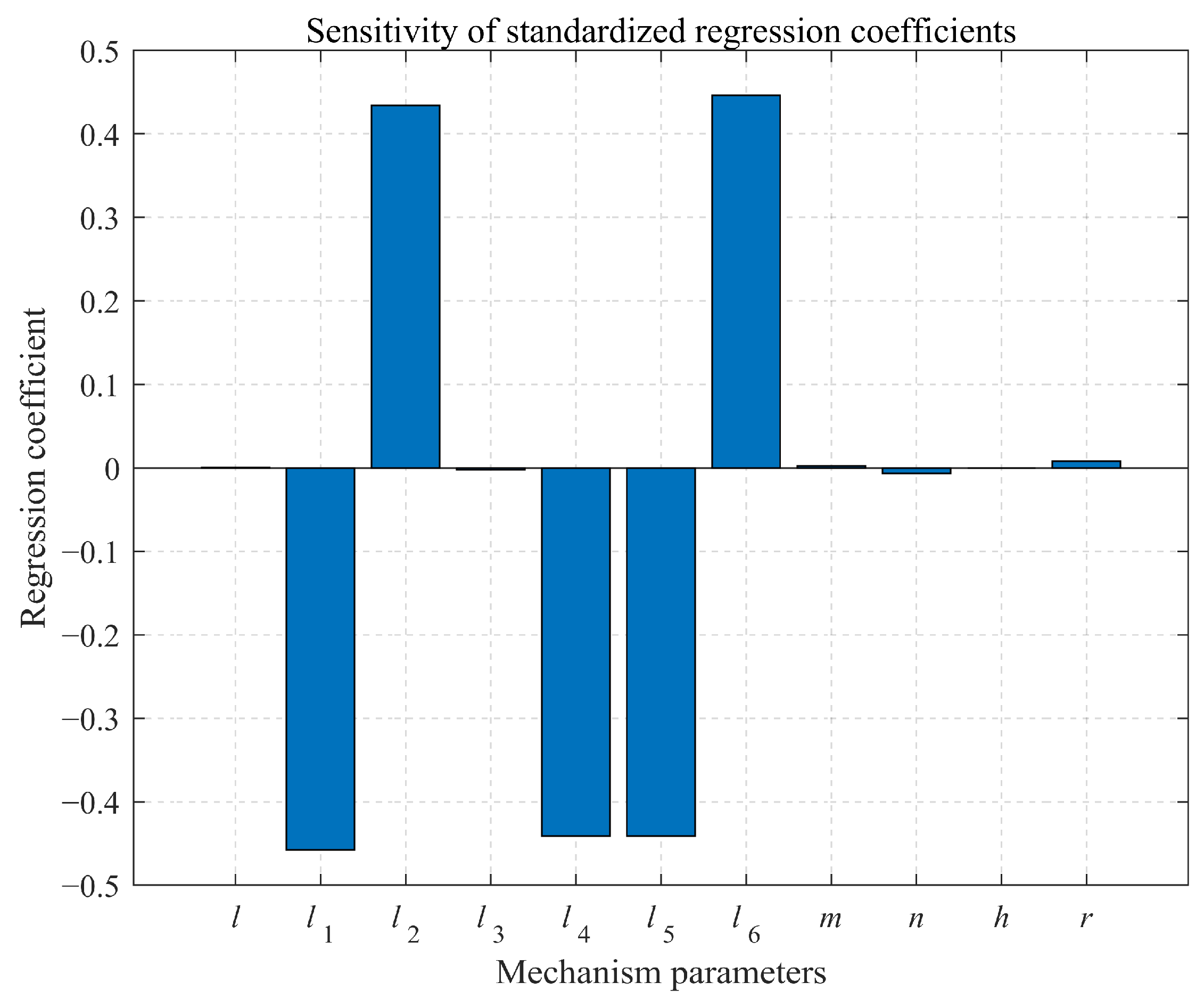
The standardized regression coefficient (${\beta }_j$) is used to evaluate the sensitivity of the mechanism parameters. In multiple regression analysis, standardized regression coefficients are obtained by converting both independent and dependent variables into standard scores (z-scores) before performing regression. This process eliminates the influence of variable dimensions, allowing for direct comparison of the effects of independent variables with different units on the dependent variable and reflecting the relative impact of each independent variable on the dependent variable.

The specific calculation method is as follows:

$${\beta }_j=b_j\cdot {\displaystyle \frac{S_{x_j}}{S_y}}$$

(35)

where $b_j$ is the raw regression coefficient, $S_{x_j}$ is the sample standard deviation of the independent variable $x_j$, and $S_y$ is the sample standard deviation of the dependent variable y.

Using this method, the parameter sensitivities for the kinematic and static models of the mechanism are calculated, and the plots of the mechanism parameter sensitivities are obtained, as shown in Figure 6 and Figure 7.

Based on the sensitivity of the mechanism’s motion accuracy, the sensitivity values of $l_3$ and $m$ are the largest, while those of l, n, h, and r are relatively small, all less than 0.01. From the sensitivity of resistant force, the sensitivity values of $l_1$, $l_2$, $l_4$, $l_5$, and $l_6$ are relatively high, whereas those of l, $l_3$, m, and h are small, all below 0.01. Notably, the parameters l and h exhibit low sensitivity to both motion accuracy and resistant force, regardless of the performance metric.

In summary, since the parameters l and h have minimal error effects and low sensitivity values for both motion accuracy and resistant force, subsequent analysis will focus on optimizing the key parameters identified via sensitivity analysis. This approach not only reduces the complexity of the optimization problem, but also enhances efficiency and improves model performance.

5. Multi-Objective Optimization Method Considering Force Transmission Performance

5.1. Multi-Objective Optimization Strategy

The guide vane adjusting mechanism studied in this paper is a single-stage mechanism with a relatively simplified design process. The key lies in determining the required blade rotation angle and establishing a correspondence between actuation and blade rotation, enabling the blade to rotate according to predefined adjustment rules under the mechanism’s actuation to achieve the design objectives. To ensure stability under complex conditions, motion accuracy must be prioritized during the design.

The force transmission performance of the guide vane adjusting mechanism directly impacts its operational efficiency, reliability, and response speed. Retarding forces in the mechanism not only reduce the force transmission efficiency, but also may cause a series of issues, including accuracy degradation, overload damage, wear fatigue, and response delays. To mitigate these negative effects, effective design and maintenance measures are essential. In practical applications, the mechanism must adapt to complex external environments while maintaining high precision and reliability for long-term stable operation.

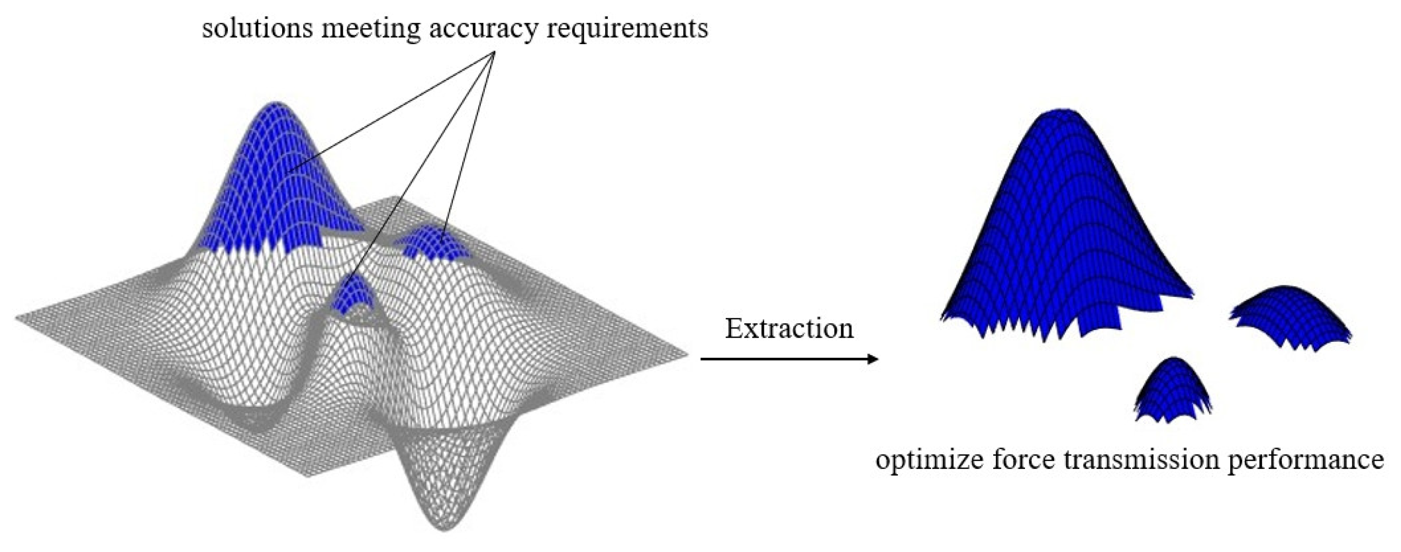
Unlike traditional multi-objective optimization, the objectives in this study do not have a parallel relationship and cannot be directly optimized through mutual coordination. The optimization requires first ensuring accuracy control before further optimizing other objectives. Therefore, developing an effective optimization strategy is critical. Common multi-objective optimization strategies include the goal weighting method and hierarchical optimization. The goal weighting method combines multiple objective functions into a single weighted objective, indirectly optimizing other objectives by solving this composite target. This approach is computationally straightforward and intuitive, but requires careful weight adjustment and may struggle to handle complex conflicts between objectives, potentially missing the optimal solution. Hierarchical optimization prioritizes objectives by importance and optimizes them sequentially: first optimizing the most critical objective to derive solutions meeting its constraints, then optimizing secondary objectives. This method ensures primary objective optimization while balancing other targets. Moreover, the goal weighting method makes it difficult to control the weights between the precision optimization objective and the force transmission performance optimization objective, which tends to result in suboptimal optimization outcomes and may require substantial time for debugging. In contrast, the hierarchical optimization method avoids this issue.

Through comparative analysis, hierarchical optimization is selected as the multi-objective optimization strategy for this study. As shown in Figure 8, all grids represent the combinations of parameter variables that can form the mechanism under the current constraints. The process first filters the parameter combinations that satisfy the accuracy requirements from all possible candidates, then optimizes the force transmission objectives within this subset to ultimately obtain the optimal solution meeting all objectives.

5.2. Multi-Objective Optimization Model

A multi-objective optimization problem refers to a situation where, based on multiple design objectives, there are multiple parameters that can be optimized around these objectives. By adjusting the combinations of these parameters, the most reasonable values of the objective functions are sought. A multi-objective optimization problem typically consists of three parts: parameters to be optimized, objective functions, and constraint conditions.

During the design and optimization of a mechanism, after constructing the kinematic and static models, in-depth analysis of the mechanism can be carried out through the forward and inverse kinematic solutions. The forward and inverse kinematic solutions have significant application value in aspects such as the motion control, trajectory planning, and kinematic optimization of the mechanism. The forward kinematic solution means that, given the types of each joint, the dimensions between adjacent joints, and the relative motion amounts between adjacent joints, the position and orientation of the end-effector of the mechanism in a fixed coordinate system are solved. The inverse kinematic solution, on the other hand, is to deduce the positions of each joint given the position and orientation of the end of the mechanism. The inverse kinematic solution is particularly important because it enables the mechanism to accurately adjust the positions of each joint according to the given target’s position and orientation, thus enabling the mechanism to complete tasks more accurately and flexibly.

In the precision optimization analysis of the guide vane correcting element, the relationship between the input and output can be calculated through the positions of each joint and the lengths of each component. This is the forward kinematic solution, denoted as $\theta =g\left({\alpha }_i,x\right)$, where $\mathsf{\theta }$ is the output angle, that is, the blade rotation angle, ${\alpha }_i$ represents the position information of each joint and the length information of each component, and $\mathrm{x}$ is the input, namely the elongation of the actuating cylinder. In the subsequent optimization process, the inverse kinematic solution model will be adopted to optimize the motion precision, denoted as $x=h\left({\alpha }_i,\theta \right)$. The static model will be used to optimize the force transmission performance, with the end output as the optimization target, to optimize the joint positions and the lengths of each component.

First, identify the optimization parameters ${\alpha }_i$ of the multi-objective optimization model, which serve as the independent variables in the optimization problem. These parameters primarily include joint positions and link lengths. By incorporating the sensitivity analysis results from the previous sections, they can be represented as follows:

$${\alpha }_i={\left[l_1,l_2,l_3,l_4,l_5,l_6,m,n,r\right]}^T$$

(36)

Next, construct the objective function of the multi-parameter optimization model. It is necessary to determine the design objectives of the mechanism. According to the optimization strategy introduced above, first construct the objective function for precision control. Based on the motion law of the current guide vane adjusting mechanism, it is known that the input and output are approximately linearly related. Suppose that the mechanism has n design points, denoted as ${\rho }_1$, ${\rho }_2$…${\rho }_n$, ${\rho }_n$, as the maximum opening angle. Due to the approximate linear relationship between the input and output, as long as the linear relationship between the two is strong enough, under the premise of precision control, the blade rotation angle can be accurately controlled to reach the design point by controlling the elongation of the actuating cylinder. The optimal value can be set as making the linear relationship between the mechanism’s input and output the strongest. Here, the calculation is based on the inverse kinematic solution model, that is $x=h\left({\alpha }_i,\theta \right)$. It can be seen that the actual values calculated in this way will be scattered points. Therefore, the evaluation index is defined as the Root Mean Square Error (RMSE). The reference-predicted value is the ideal linear straight line. It is known that the smaller the value of the RMSE, the better the degree of linear fitting, and the more ideal the precision control. The objective function can be expressed as follows:

$$\beta =\sqrt{{\displaystyle \frac{{\displaystyle \sum _{i=1}^n{\left(x_{pi}-x_{ai}\right)}^2}}{n}}}$$

(37)

where $\beta$ represents the value of the Root Mean Square Error. The coordinate values of the actual elongation of the actuating cylinder and the blade rotation angle are defined as $({\theta }_a,x_a)$, and the coordinate values of the predicted elongation of the actuating cylinder and the blade rotation angle are defined as $({\theta }_p,x_p)$. n is the number of coordinate points to be calculated, which can be selected independently.

Then, construct the objective function for the force transmission performance. To improve the force transmission performance of the mechanism, the average value of the driving force can be reduced through optimization, and at the same time, the amplitude of the driving force change can be decreased. Therefore, it can be expressed as follows:

$${\overline{F}}_Q={\displaystyle \frac{{\displaystyle \sum _{i=1}^n{F}_{Qi}}}{n}}$$

(38)

$$R=F_{Q\max }-F_{Q\min }$$

(39)

Finally, construct the constraint conditions of the multi-parameter optimization model. The constraint conditions are the restrictions and constraints on the parameters to be optimized in the optimization problem. In the multi-parameter optimization model of the guide vane adjusting mechanism, the mechanism interference, spatial position, and structural dimensions, etc., are the key to establishing the constraint equations. Different structural parameters lead to different constraint conditions, and the final optimization results also vary greatly. The constraint equations can be expressed as follows:

$${\alpha }_{i\min }\le {\alpha }_i\le {\alpha }_{i\max }$$

(40)

The establishment of constraints will be elaborated in the subsequent case analysis. Based on the above-mentioned analysis process, the entire optimization process can be refined, and the optimal parameter combination can be obtained.

5.3. Global Optimization Design Solution

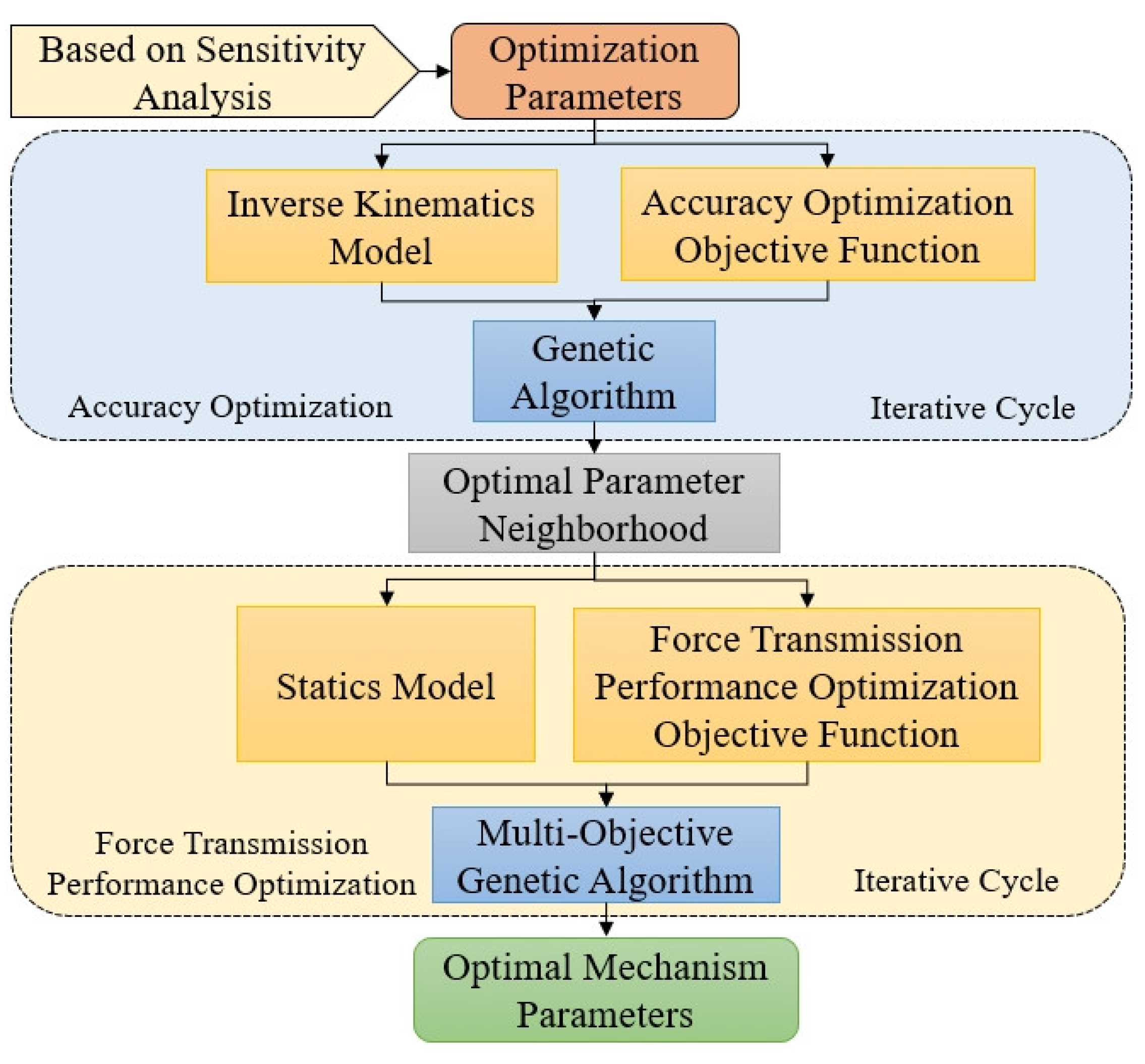
Based on the solution strategy for the multi-objective optimization design of the adjusting mechanism, a multi-objective optimization design method for the mechanism considering the force transmission performance can be proposed. The optimal solutions of the multi-objective optimization model can be solved using global optimization algorithms. This paper employs a multi-objective genetic optimization algorithm as the calculation method to solve the optimization model. Its fundamental idea is to simulate genetic operations (selection, crossover, and mutation) to search for a set of “Pareto optimal solutions” in the objective space, forming a Pareto front that reflects the optimal trade-offs between objectives and providing an efficient solution set search tool for complex systems. The core lies in balancing the convergence (approximating the true Pareto front) and diversity (uniform distribution of solutions), and through mechanisms such as non-dominated sorting and crowding distance calculation, it identifies optimal compromise solutions among multiple conflicting objectives. It can solve any kind of practical problem and has a broad application value. The solution process in this paper is shown in Figure 9.

Based on the mechanism’s inverse kinematic equations, a precision optimization model was established. Genetic algorithms were employed to rapidly compute and solve for the neighborhood of optimal mechanism parameters. Given that the kinematic model of the guide vane adjusting mechanism is analytical, the kinematic optimization model demonstrates a fast computation speed and high optimization design efficiency. Subsequently, a force transmission performance optimization model was developed using the mechanism’s static model. Taking the data obtained from precision optimization as the initial values, a multi-objective genetic optimization algorithm was applied to search for the optimal force transmission performance while ensuring mechanism precision.

6. Case Analysis

Take the simplified model shown in Figure 1 as an example of optimization design. Based on the multi-objective genetic algorithm, the global optimal mechanism parameters are solved. Under the current mechanism model, the original parameters of each mechanism are shown in

Table 3. Original parameter table of the mechanism.

Parameter	$\mathit{l}$	${\mathit{l}}_1$	${\mathit{l}}_2$	${\mathit{l}}_3$	${\mathit{l}}_4$	${\mathit{l}}_5$	${\mathit{l}}_6$	m	n	h	r
dimension/mm	320	70	70	74	460	75	432	74	0	0	70

. It is required that in the current intermediate position, the blade rotation angle is ±10°and the actuator elongation is ±14 mm.

6.1. Parameter Optimization Objectives

At present, the mechanism is at the mid-position of its motion, and the guide vane angle of the mechanism is also at the mid-position. In the kinematic and static models of the mechanism established previously, optimization is carried out with this position as the initial position. The mechanism needs to move from this position to the maximum blade rotation angle position of 10° and the minimum blade rotation angle position of –10°. During the kinematic process, these two processes are approximately symmetric. Therefore, in kinematic optimization, for the convenience and speed of calculation, only the process of moving from this position to the state where the actuator extends to 14 mm is selected. So, for the optimization of mechanism accuracy, the optimization goal is that the curves of the actuator elongation and the blade rotation angle obtained from the motion should be fitted to a straight line to the greatest extent.

$$x_p=1.4{\theta }_p$$

(41)

taking the Root Mean Square Error $\beta$ between the two as the objective function for accuracy optimization. After considering the force transmission performance of the mechanism, assume that the mechanism is driven by a single actuator, and that the sum of the $M_Y$ forces on each blade is 500 N·m. Using $\overline{F_Q}$ and R as the objective functions for optimization, analyze the above-mentioned optimization objectives.

6.2. The Establishment of Parameter Constraints

According to the optimization objectives, the input and output parameters of the regulating mechanism are predefined fixed parameters, while the remaining parameters are subject to optimization. Through comprehensive consideration of the mechanism installation space and potential component interferences, and combined with the results of sensitivity analysis, the upper and lower bounds for the mechanism design parameters are provided in

Table 4. Upper and lower limits of mechanism design parameters.

Mechanism Parameters	Lower Limit of Parameters/mm	Upper Limit of Parameters/mm
$l_1$	60	80
$l_2$	60	80
$l_3$	70	80
$l_4$	450	470
$l_5$	70	80
$l_6$	420	440
m	70	80
n	−2	2
r	70	80

.

After obtaining the upper and lower limit constraints of the mechanism parameters, the next step is to determine the constraint relationships among the mechanism parameters. As mentioned above, the kinematic inverse solution model is used for the optimization analysis of the mechanism. Therefore, the constraint relationships among the mechanism design parameters mainly come from the correlation relationships in the kinematic inverse solution model. By analyzing the analytical expressions of the kinematic inverse solution model, the interrelationships and constraint conditions among various parameters can be obtained. Based on these constraint relationships, further optimization analysis of the mechanism can be carried out to ensure that the design parameters meet the performance requirements and achieve the goals.

6.3. Parameter Optimization Solving

By leveraging the above objective function and constraint relationships, the complex mechanism parameter optimization problem is transformed into a mathematical model problem. Following the optimization of the mechanism’s force transmission performance, optimization calculations were performed using a multi-objective genetic algorithm. During accuracy optimization, the iteration number is set to 5000 to find more solutions meeting the accuracy requirements. Subsequently, force transmission performance optimization is carried out by evaluating all eligible solutions obtained from the above process, thereby determining the mechanism parameter values under the optimal force transmission performance. Based on the described solution process, three groups of optimized data were obtained, as presented in

Table 5. Mechanism parameter table after accuracy-only optimization.

Parameter	${\mathit{l}}_1$	${\mathit{l}}_2$	${\mathit{l}}_3$	${\mathit{l}}_4$	${\mathit{l}}_5$	${\mathit{l}}_6$	m	n	r
group 1/mm	68.40	62.08	77.59	453.07	67.99	420.13	77.49	0.73	66.91
group 2/mm	75.67	72.52	78.24	464.39	70.71	425.34	78.23	−1.68	72.94
group 3/mm	70.71	73.54	74.86	461.31	79.52	437.40	74.83	1.72	77.75

.

6.4. Result Analysis

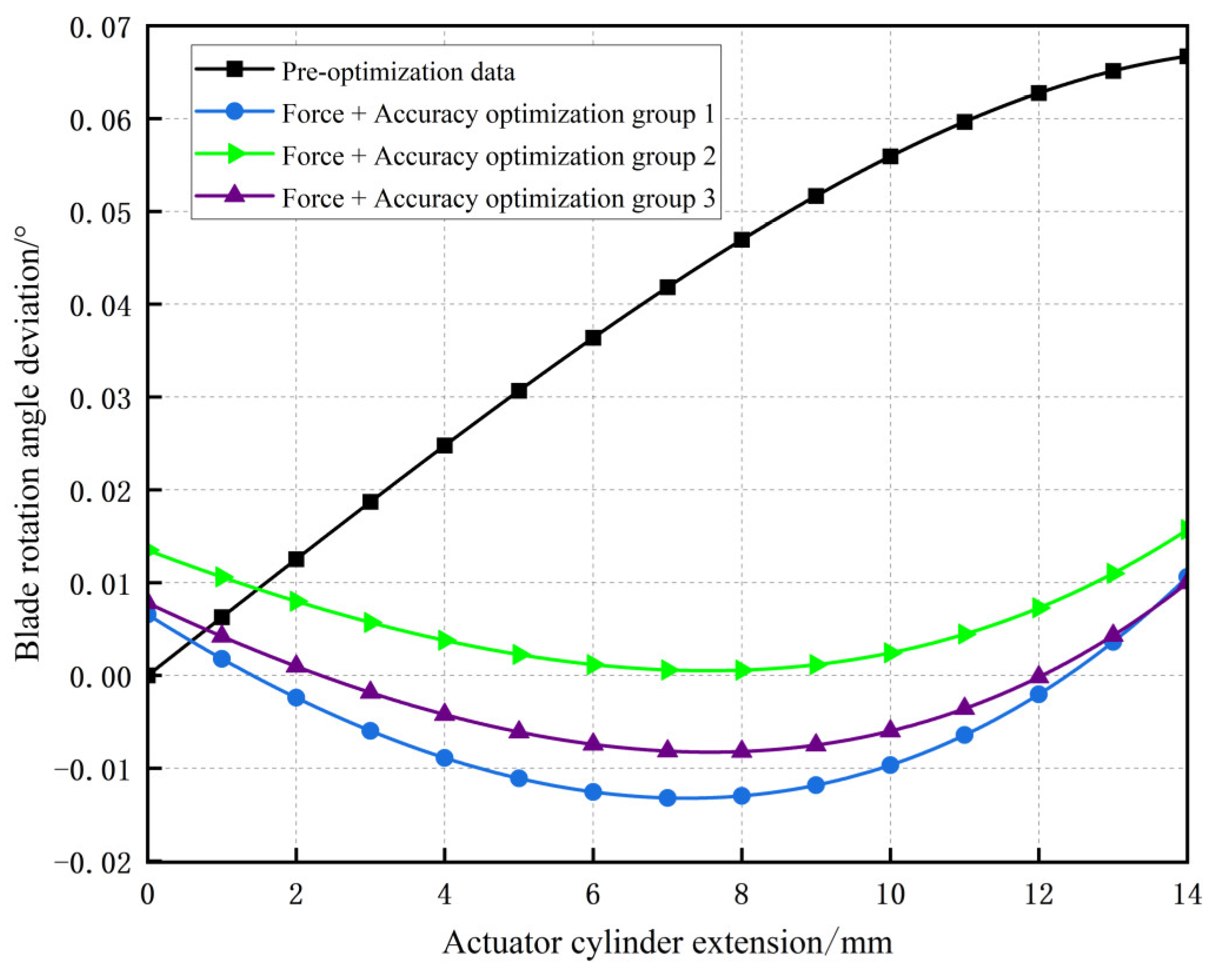
By combining the results obtained before and after optimization, based on the analytical kinematic model, the deviation values between each curve and the theoretical curve are calculated, and the deviation curves are obtained, as shown in Figure 10.

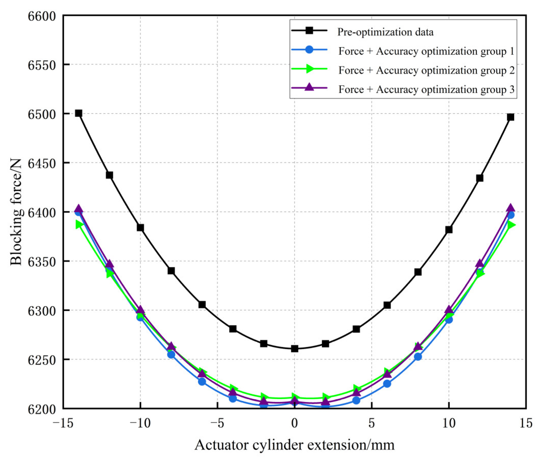
The precision deviations of the three sets of optimized results exhibit certain differences, but the deviation values (both peak and average) relative to the theoretical curve are significantly lower than those of the case data, indicating a substantial improvement in the blade rotation angle accuracy. Subsequently, based on the static model, the relationship curve between the actuator cylinder extension and blocking force was derived, as presented in Figure 11, with the key data listed in

Table 6. Key data of the analytical model blocking force.

	Pre-Optimization Data	Group 1 Data	Group 2 Data	Group 3 Data
maximum value/N	6563.33	6399.8	6387.24	6403.39
minimum value/N	6260.87	6201.84	6210.22	6205.46
difference value/N	302.46	197.96	177.02	197.93
mean value/N	6354.48	6260.06	6265.56	6266.67

.

Following optimization considering the force transmission performance, all data points on the blocking force curve have been improved. Notably, the difference between the maximum and minimum values has been significantly reduced, effectively minimizing blocking force fluctuations and further validating the effectiveness of optimizing the force transmission performance.

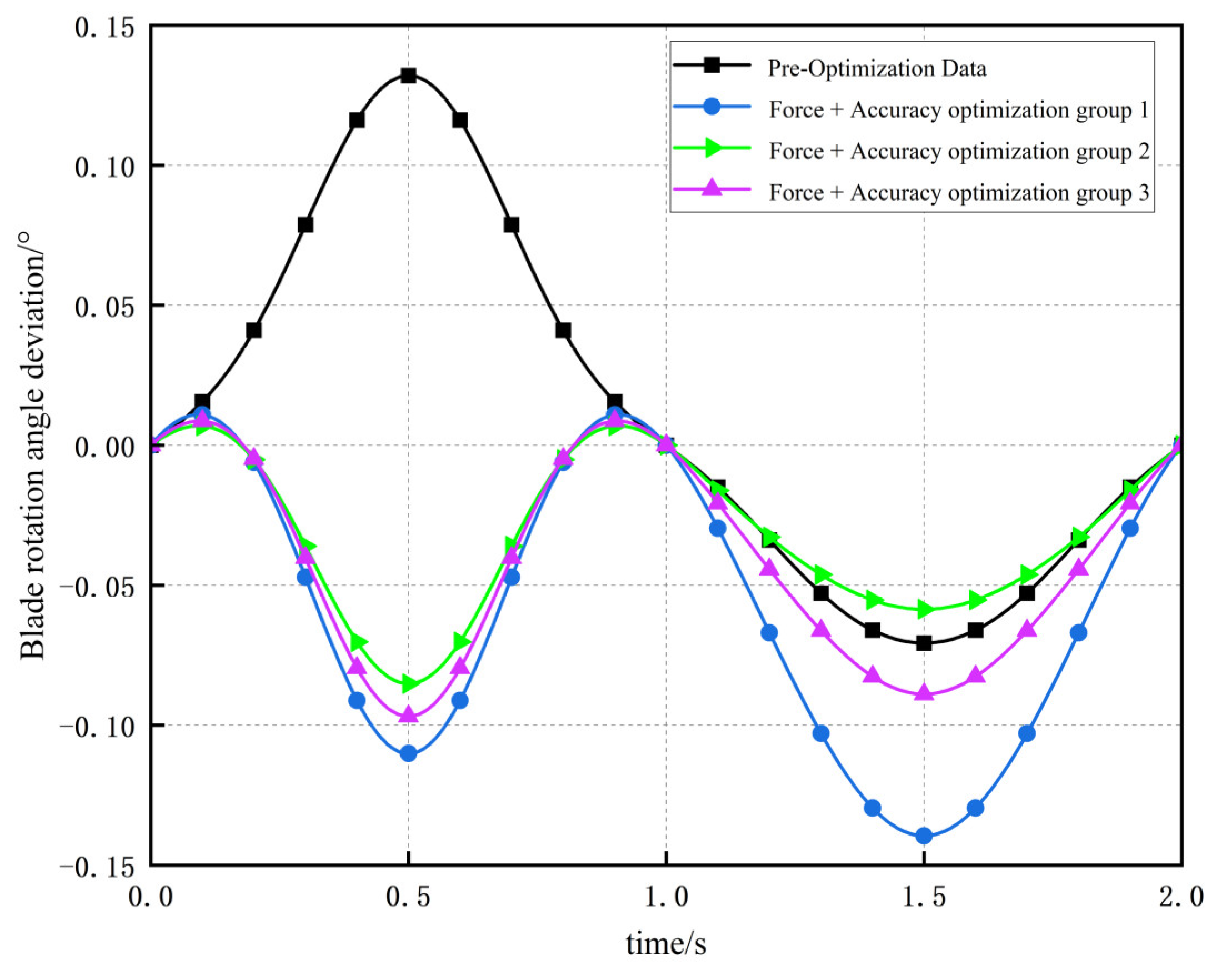
To verify the correctness of the analytical model and the validity of the optimized design, the pre- and post-optimization mechanisms were modeled and imported into ADAMS for simulation analysis. A sinusoidal displacement drive of $14\times \sin (180°\times \mathrm{TIME})$ was applied, which allows for the observation of the mechanism’s complete motion over one cycle and the verification of whether the blade achieves the designed rotation angle. By using a full rigid-body model with specified kinematic pairs (neglecting motion pair characteristics’ impacts on blocking force), relevant results were obtained.

Deviations between pre- and post-optimization data and the theoretical blade rotation angle curve ($14\times \sin (180°\times \mathrm{TIME})$ based on the drive curve) were calculated, with the deviation curves shown in Figure 12.

At 0.5 s and 1.5 s, the actuator reaches its maximum and minimum stroke positions, where all four datasets exhibit the largest deviation values. Post-optimization Groups 2 and 3 demonstrate improved accuracy, while Group 1’s deviation values remain comparable to the pre-optimization data, indicating minimal optimization effects.

Subsequently, the optimization results of blocking force are analyzed, as shown in Figure 13, with the key data presented in

Table 7. Key data of the simulation model blocking force.

	Pre-Optimization Data	Group 1 Data	Group 2 Data	Group 3 Data
maximum value/N	6369.00	6286.40	6309.74	6301.62
minimum value/N	6249.77	6181.87	6198.9	6189.45
difference value/N	119.23	104.53	110.84	112.17
mean value/N	6314.16	6239.68	6258.22	6252.22

.

The simulation model results align generally with the analytical model results, both confirming the necessity and effectiveness of the optimization design considering the force transmission performance. However, minor numerical discrepancies exist. Analysis attributes these differences to two factors: (1) simplifications in the analytical model at the linkage ring, which inherently involves complex spatial motion; (2) the analytical model’s inability to account for the physical properties of links and inertial forces during motion, both of which influence the results in ADAMS multi-body dynamics simulations.

The three optimized datasets exhibit distinct characteristics. The final optimization results can be selected based on weighted priorities between accuracy and blocking force, or through iterative optimization comparisons. According to the three optimized results presented here, the Group 2 data are recommended as the final choice.

Overall, the multi-objective optimization of the guide vane adjusting mechanism proposed in this paper achieves superior design for both the accuracy and force transmission performance. Compared to the pre-optimization data, the motion accuracy improves by 38.4% at maximum actuator extension and 14.3% at minimum actuator extension. Additionally, the maximum blocking force difference decreases by 7.0%, with reductions in both the peak and average values, demonstrating strong practical utility.

7. Conclusions

This paper presents an optimization design method for the inlet guide vane adjusting mechanism, which establishes a multi-objective optimization strategy prioritizing accuracy optimization and considering force transmission performance. Using the established kinematic and static models of the mechanism as the optimization framework, the optimization parameters are determined based on the sensitivity analysis results of both models, along with the constraint conditions. The global multi-objective optimization design of the mechanism is then conducted using a multi-objective genetic algorithm. By comparing the case data with the optimization results considering force transmission performance, it is shown that the motion accuracy is improved by 38.4% at the maximum actuator extension and 14.3% at the minimum actuator extension compared to the pre-optimization data. The maximum difference in the blocking force is reduced by 7.0%, with both the peak and average values also decreasing. These results demonstrate that the optimized design enhances both the motion accuracy and blocking force stability, verifying the effectiveness and practicality of the proposed models.

The method effectively achieves global optimization design considering both mechanism precision and stagnation force, minimizing the jamming risks caused by excessive stagnation force due to design factors. This study provides a novel approach for the global optimization design of the guide vane adjusting mechanism.