Transient High-Frequency Electromagnetic Force Calculation for Linear Induction Motors Under Pulse Width Modulation Current Excitation

Abstract

Because of their transient working mode and end effects, it is particularly difficult to compute high-frequency electromagnetic forces on linear induction motors under PWM current simulation. The current methods for computing high-frequency electromagnetic forces in transient operating conditions are computationally expensive and have limited practicality. To deal with these issues, this paper introduces a non-periodic transient high-frequency electromagnetic force calculation model. Firstly, an examination of a linear induction motor under PWM currents demonstrates that the transient magnetic field calculation issue in a linear induction motor can be simplified to a periodic boundary steady-state magnetic field calculation problem. Based on this, a 2D magnetic field analytical model is established for high-frequency magnetic field calculation. Subsequently, a hybrid approach employing both finite element analysis and analytical methods is employed to compute the transient magnetic field. Finally, electromagnetic forces are calculated across the entire frequency spectrum, and the correctness of the model is validated indirectly through motor vibration experiments. This model offers faster and more accurate results than finite element analysis, making it suitable for application in the iterative stages of motor optimization design and applicable to rotary induction motors.

1. Introduction

Due to their straightforward mechanical structure and high reliability, linear induction motors (LIMs) are receiving increasing attention in the fields of electromagnetic launch, rail transportation, and logistics transmission [1,2,3,4,5]. LIMs are mostly driven by inverters, and since the output current of the inverter contains a large amount of PWM harmonics, it will cause high-frequency vibrations in the motor product [6,7,8], which will eventually lead to mechanical damage and fatigue failure. LIMs have a unique structure, making the electromagnetic vibration theory of rotary motors not directly applicable to LIMs. The distinction between LIMs and rotary motors primarily lies in two aspects: firstly, the shorter travel distance of LIMs, with most operating in non-periodic transient conditions, and secondly, the end effects, which cause distortion of the magnetic field (MF) [9,10]. Due to the above MF characteristics, which differ from those of rotating motors, the study of vibrations in LIMs is more complex. On the other hand, there is also a distinction in their applications. In wave power generation [11,12,13,14], linear motors directly convert the wave’s reciprocating linear motion into electrical energy without intermediate conversion mechanisms such as gears/screws, which gives them the advantages of compact structure, high efficiency, and low maintenance costs, whereas rotary motors need to convert the wave’s linear motion into rotary motion, which leads to transmission loss and mechanical wear-and-tear problems. In monorail transportation [15,16,17,18], linear motors directly drive the linear motion of the vehicle, without a transmission mechanism, and with high climbing capacity; in contrast, rotary motors need gears/screws to convert rotational motion to linear motion, and there are transmission losses, but the technology is mature and low-cost. In launching equipment [19,20], linear motors generate electromagnetic thrust directly and achieve high speed, while rotary motors require mechanical conversion and have a mature structure but low efficiency.

Calculating the electromagnetic force (EF) is important in researching the electromagnetic vibration of motors, and the first step in calculating EFs is to compute the MF. For the calculation of the MF inside the motor, the mainstream methods currently include the magnetic potential method [7,21], the semi-analytical subdomain method [22,23,24], the conformal mapping method [25,26], and FEA [27,28,29]. The magnetic potential method relies on the winding configuration of coils to compute the spatial magnetic flux distribution. This method involves linearized processing and cannot account for the effects of core saturation, resulting in relatively low accuracy. The subdomain method divides the MF solving region into several subdomains, combines boundary conditions at the interfaces of each subdomain, and directly solves the Laplace or Poisson equations. This method establishes analytical relationships between MF distribution and motor structural parameters, with clear physical significance. However, it involves some difficulty in formulating and solving partial differential equations. The semi-analytical subdomain method emerged to simplify the analytical solving process, as it involves complex derivations and large formulas, ultimately resorting to numerical computations in the final solving stage to simplify the formulas. Comparing the subdomain method with FEA, the former overcomes topological constraints and exhibits robustness to geometric models. Moreover, the computational time cost of using the semi-analytical subdomain method is much lower than that of FEA, but the subdomain method still cannot solve nonlinear problems.

Except for FEA, the methods listed above are acceptable for steady-state solutions. FEA is most appropriate for transient analysis. However, the computational cost of FEA is quite expensive for large-scale motor models. For the problem addressed in this paper, solving the transient MF problem with FEA under PWM current excitation is challenging, because the PWM current frequency is too high, making FEM simulation completely impractical if the time step for the solution must be extremely small.

In order to address the high-frequency EF issue of LIMs operating under inverter drive in transient conditions, this paper comprehensively considers factors such as PWM currents, non-periodic transient conditions, and end effects, and proposes a fast approach to the EF calculation of LIMs. Firstly, the electromagnetic characteristics of LIMs under PWM high-frequency excitation are analyzed, and it is determined that under high-frequency excitation, the end effects of LIMs can be ignored and the transient process of LIMs is short. Therefore, the challenge of calculating high-frequency MF for transient operation may be reduced to that of calculating high-frequency MF for steady-state operation with periodic boundaries. Then, the low-frequency MF is computed by FEA, whereas the high-frequency MF is calculated analytically. Subsequently, based on the principle of MF superposition, the whole MF inside the motor is generated through superposition at temporal and spatial coordinate points, and the EFs of various motor components are calculated. Finally, the EFs are applied to a dynamic model of an LIM to calculate the electromagnetic vibrations, which are compared with the experimental vibrations to indirectly validate the accuracy of the EF calculation results. A flowchart of the research methodology and research approach of this paper is shown in Figure 1.

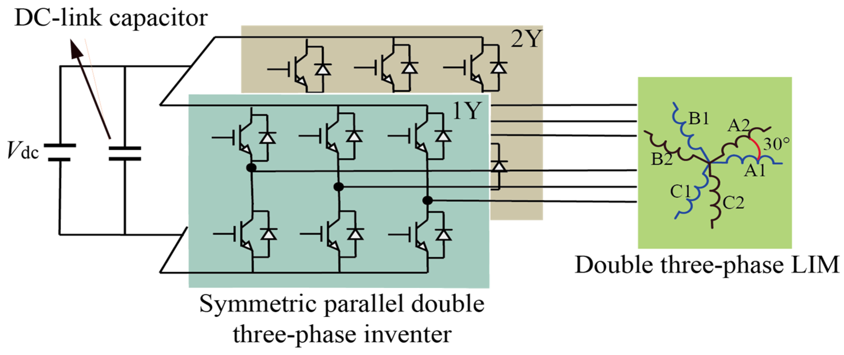
2. System of Double Three-Phase LIM

The mover of the LIM is integrated with the piston, where the mover’s motion drives the piston’s movement. This configuration is applicable to underwater propulsion, applications requiring reciprocating piston motion for gas compression, and high-impact scenarios demanding short-distance actuation, such as offshore pile drivers.

The double three-phase LIM is powered by a symmetric parallel double three-phase inverter, which is composed of two identical three-phase full-bridge inverters connected in parallel, and its topology is illustrated in Figure 2. It consists of two independent three-phase full-bridge inverters connected in parallel. On the AC side, they are linked to the two independent three-phase windings of the LIM. On the DC side, a steady DC power source is connected in parallel with a smoothing capacitor to reduce DC-side current fluctuations. Both Inverter 1 and Inverter 2 employ SPWM modulation.

The structure of the double three-phase LIM is shown in Figure 3, and the mechanism and motion process of the LIM are shown in Figure 4. The mover of the LIM is integrated with a piston, which can compress water or gas, and both ends of the piston are in contact with the stator to play a supporting role. The mover moves in a straight line under the action of electromagnetic forces in the windings and is supported by sliding friction during the movement. The position of the mover is measured by means of a pull-cord-type position sensor, which detects the position of the pull-cord to obtain the position of the mover. It features a long secondary and short primary structure, with primary motion. The primary core is designed without slots to reduce spatial cogging harmonics. Two independent windings on the primary core are Y-connected with a 30° spatial phase difference. The secondary component is composed of copper layers and an iron core, the primary and secondary cores are laminated and stacked circumferentially, with the specific structural parameters detailed in

Table 1. Structural parameters of LIM.

Parameter	Symbols	Value	Unit
Primary core thickness	hpc	40	mm
Primary length	lp	660	mm
Winding thickness	hco	15	mm
Air gap	ge	3	mm
Conductive layer thickness	hcl	10	mm
Back iron thickness	hbi	30	mm
Pole pitch	τ	155	mm
Conductive layer conductivity	σcu	6.6 × 106	S/m
Pole pair number	P	2	--

.

3. Characteristics of LIM Under High-Frequency Current Excitation

3.1. Characteristics of End Effect Under High-Frequency Current Excitation

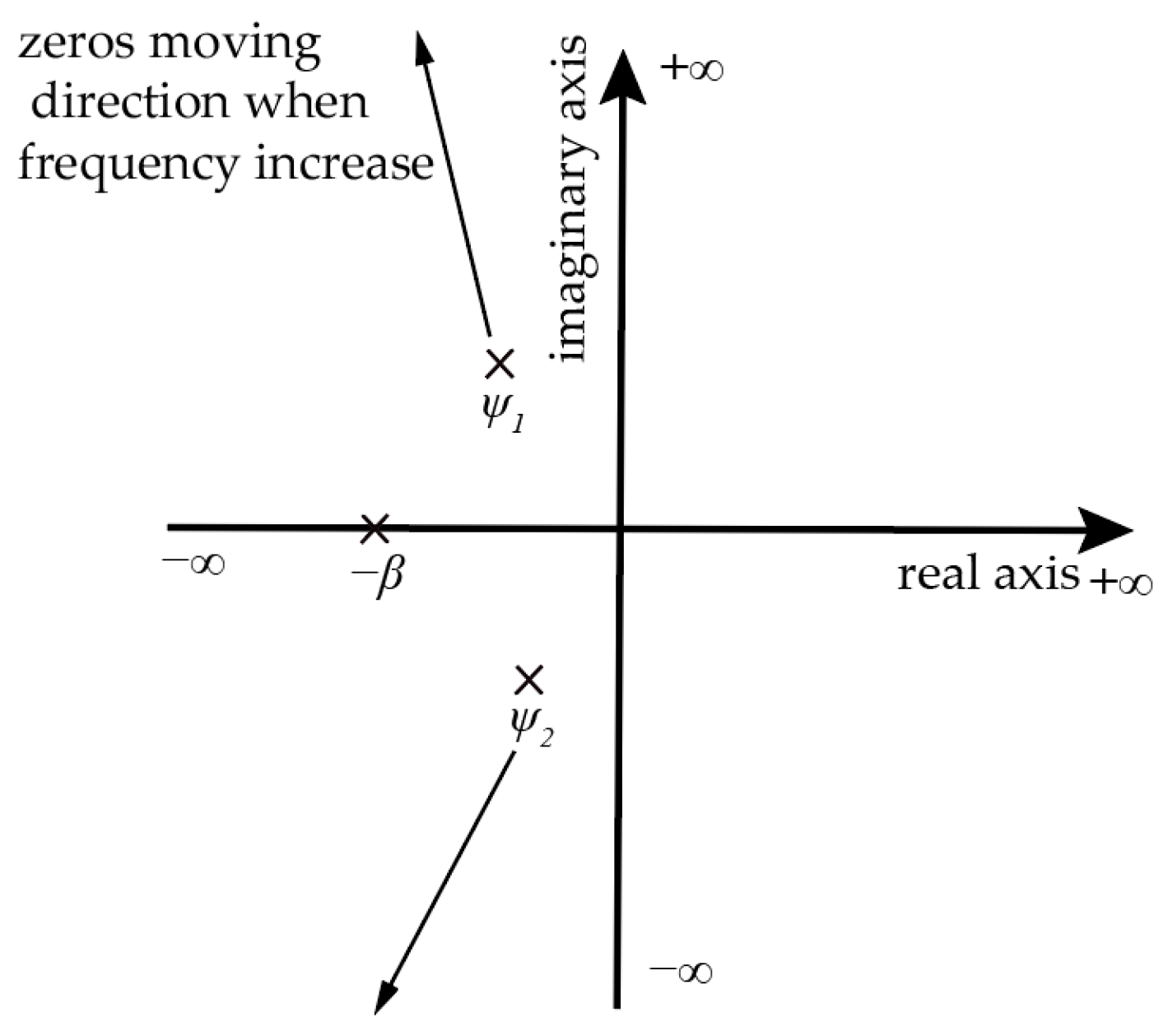
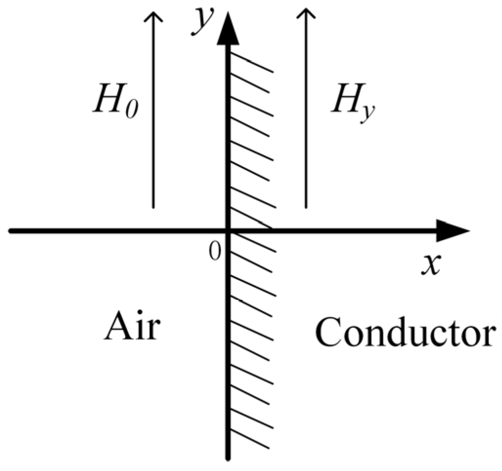
3.1.1. Theoretical Analysis

Referring to the analytical formulation in [30], MF modeling of the LIM was conducted. The motor was initially divided into four subdomains, namely the secondary back iron (Subdomain 1), the conductive layer (Subdomain 2), the air gap (Subdomain 3), and the primary core (Subdomain 4), and we assumed that the winding was a current layer with no thickness; the subdomain names of the LIM can be found in the 2D model in Figure 2. By employing the governing equations and boundary conditions applicable to each subdomain, MF equations for each subdomain were derived. Within the conductive layer, the MF equations along the x-axis and y-axis directions are expressed as (1) and (2), respectively, with the x-axis’ positive direction corresponding to the direction of motion of the mover.

$$B_{\mathrm{x}2}={\mu }_{0}J\left[\begin{array}{l}{\displaystyle \frac{-\exp \{-j(\beta +{\psi }_2)L\}{\varphi }_2\sinh \{{\varphi }_2(h_{\mathrm{cl}}+y)\}\exp (j{\psi }_{2}x)}{({\psi }_2+\beta )Q^{\prime }({\psi }_2)}}\\ -{\displaystyle \frac{{(\varphi )}_{-\beta }\sinh \{(h_{\mathrm{cl}}+y){(\varphi )}_{-\beta }\}\exp (-j\beta x)}{Q(-\beta )}}\\ -{\displaystyle \frac{{\varphi }_1\sinh \{{\varphi }_1(h_{\mathrm{cl}}+y)\}\exp (j{\psi }_{1}x)}{({\psi }_1+\beta )Q^{\prime }({\psi }_1)}}\end{array}\right]$$

(1)

$$B_{\mathrm{y}2}=j{\mu }_{0}J\left[\begin{array}{l}{\displaystyle \frac{-\beta \cosh \{(h_{\mathrm{cl}}+y){(\varphi )}_{-\beta }\}\exp (-j\beta x)}{Q(-\beta )}}\\ +{\displaystyle \frac{{\psi }_1\cosh \{(h_{\mathrm{cl}}+y){(\varphi )}_{{\psi }_1}\}\exp (j{\psi }_{1}x)}{({\psi }_1+\beta )Q^{\prime }({\psi }_1)}}\\ +{\displaystyle \frac{{\psi }_2\exp \{-j(\beta +{\psi }_2)L\}\cosh \{(h_{\mathrm{cl}}+y){(\varphi )}_{{\psi }_2}\}\exp (j{\psi }_{2}x)}{({\psi }_2+\beta )Q^{\prime }({\psi }_2)}}\end{array}\right]$$

(2)

$$\begin{array}{l}Q({\psi }_i)={\psi }_i\sinh h_{air}{\psi }_i\cosh {\varphi }_i{h}_{cl}\\ \hspace{1em}\hspace{1em}\hspace{1em}+{\varphi }_i\cosh h_{air}{\psi }_i\sinh {\varphi }_i{h}_{cl}\end{array}$$

(3)

$${\varphi }_i=\sqrt{{\psi }_i^2+j{\mu }_i{\sigma }_i(V{\psi }_i+\omega )}$$

(4)

where μ₀ represents the permeability of air, J denotes the traveling wave’s current density, β = π/τ signifies the wave number, L stands for the primary length, ψ_i represents the zero crossing of Q(ψ_i), σ_i is the conductivity of subdomain i (i = 1, 2, 3, 4), V denotes the mover’s velocity, and ω represents the primary current’s angular frequency (for a detailed derivation of the formula above, please refer to [30]).

In (1) and (2), terms with exp(−βx) represent the fundamental wave MF, while terms with exp(jψ₁x) and exp(jψ₂x) correspond to the inlet and outlet wave MF, respectively.

Solving for the zeros of Q(ψ_i) is a complex task, and it is challenging to find these zeros through analytical methods, but it can be achieved using the Muller iterative method. The solution reveals that as the supply frequency ω increases, the zeros ψ₁ and ψ₂ move away from the real axis, as illustrated in Figure 5. This implies that the imaginary parts of the zeros ψ₁ and ψ₂ increase, which will lead to greater attenuation in the variation in exp(jψ₁x) and exp(jψ₂x) with respect to x; this manifests rapid attenuation of the inlet and outlet waves, with a relatively minor impact on the fundamental MF. Consequently, with the rise in supply frequency, the end effect weakens.

Based on derivation and analysis, it can be observed that the end effects are associated with the supply frequency. To explore the effect of supply frequency on the characteristics of end effects, the analytical model from [30] is used to compute the MF distribution at different supply frequencies. A comparison is made between the total air gap MF, inlet wave MF, and outlet wave MF at supply frequencies of 10 Hz, 100 Hz, and 1000 Hz, with a mover velocity of 4 m/s and a current amplitude of 1000 A. The results of this calculation are depicted in Figure 6. From Figure 6, it is evident that increasing the supply frequency reduces the distortion of the total air gap MF. Furthermore, the inlet wave MF and outlet wave MF exhibit increased attenuation along the x-direction. When the supply frequency reaches 1000 Hz, the total air gap MF approximates a sinusoidal waveform.

When the velocity is kept constant, the analysis mentioned above shows that as the supply frequency increase, the end effects steadily decrease. So, under PWM current excitation, the end effects can be neglected. Thus, the LIM model with open boundaries can be simplified to a model with periodic boundary conditions.

3.1.2. Verification of Analysis Results Based on FEA

To validate the replacement of the actual motor structure model with a periodic boundary model under high-frequency excitation, transient FEA models for both the actual structure and the periodic boundary structure are established in FEA software (Maxwell 2022R1) by the 2D axisymmetric transient MF solver, as depicted in Figure 7.

In the FEA models, the simulated operating conditions are transient, where the current amplitude undergoes an instantaneous rise from 0 A to 5000 A within the time interval of 0 s to 1 s. The current frequency ranges from 4 kHz to 4.02 kHz, with a simulated switching frequency of 4 kHz and a fundamental frequency of 0–20 Hz. The mover’s translational velocity is set at 4 m/s. A comparison of MF at the midpoint of the electromagnetic air gap is performed at 0.3 s, as illustrated in Figure 8.

From Figure 8a, it can be observed that there is good agreement in the y-direction MFs between the actual motor model and the periodic boundary model. However, near the end, an error of 4% is introduced due to static end effects. Similarly, there is favorable alignment in the x-direction MFs between the actual motor model and the periodic boundary model, with an error at the end measuring 4.5%, as depicted in Figure 8b.

Based on the comprehensive analysis above, under high-frequency excitation, it can be concluded that the end effects are not significant under high-frequency excitation. Consequently, the periodic boundary model can be effectively utilized for equivalent calculations of the actual structure model.

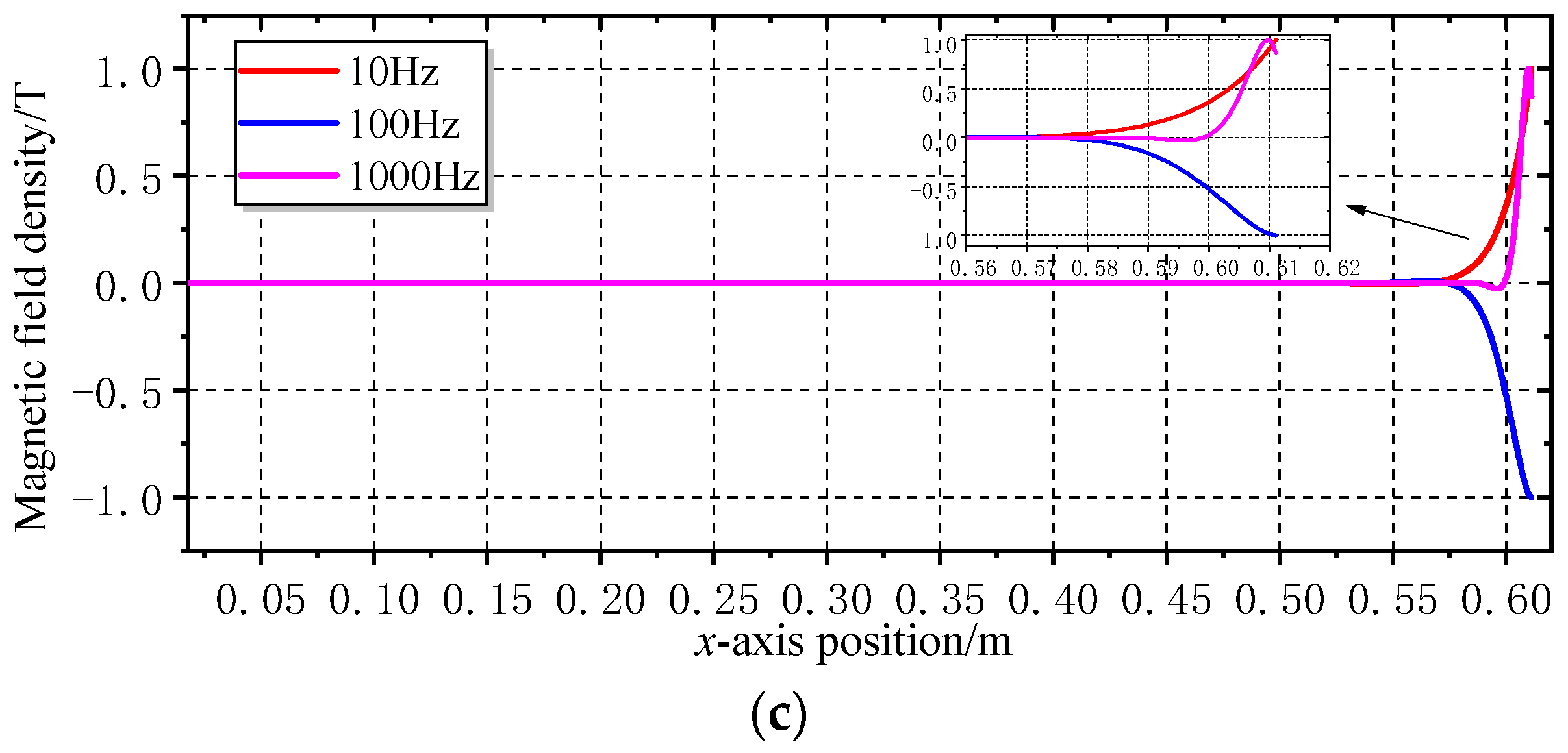
3.2. Transient Electromagnetic Characteristic Under High-Frequency Current Excitation

3.2.1. Theoretical Analysis

At low-frequency excitation, the magnetic path passes through the secondary conducting layer and the secondary core, and the whole transient electromagnetic response time of the secondary system is collectively determined by the conducting layer and the secondary core. However, under high-frequency excitation, the shielding effect of the conducting layer modifieds the magnetic path, causing the conducting layer surface and the air gap to become the primary components of the magnetic path, as illustrated in Figure 9. Therefore, under high-frequency excitation, the transient electromagnetic response time of the secondary system is primarily determined by the stable duration of eddy currents on the conducting layer. In the following sections, the establishment time of eddy currents in the conducting layer under high-frequency excitation is investigated qualitatively from a field perspective.

Due to the skin effect, induced eddy currents concentrate on the surface of the conducting layer, and the penetration depth of these eddy currents relative to their thickness is relatively small. The conducting layer can be approximated as an infinitely large conductor under high-frequency excitation. Therefore, the transient electromagnetic response time of the secondary system under high-frequency excitation can be determined by analyzing the establishment time of eddy currents in a semi-infinite conductor.

As shown in Figure 10, the structure represents a semi-infinite conductor, extending infinitely along the positive and negative halves of the y-axis, and infinitely along the positive half of the x-axis. Applying a step MF H₀(t) to the surface of the conductor, at this moment, only the MF component Hy exists in the y-direction within the semi-infinite conductor. Furthermore, Hy is a function of both x and t, denoted as H = H_y(x,t), satisfying a one-dimensional eddy-current equation.

$${\displaystyle \frac{{\partial }^2{H}_{\mathrm{y}}}{\partial x^2}}=\mu \sigma {\displaystyle \frac{\partial H_{\mathrm{y}}}{\partial t}}\left(x>0\right)$$

(5)

Based on the step magnetic field on the conductor surface, the corresponding initial and boundary conditions can be derived as follows.

• When t = 0, H_y(x,0) = 0 (except for x = 0).
• When x = 0, H_y(0,t) = H₀.

Furthermore, by utilizing Laplace transforms in accordance with the eddy-current equation, initial conditions, and boundary conditions, the induced current J_z within a semi-infinite planar region can be solved using Equation (6).

$$J_{\mathrm{z}}=-H_0\sqrt{{\displaystyle \frac{\mu \sigma }{\pi t}}}{\mathrm{e}}^{-{\displaystyle \frac{\mu \sigma }{4t}}{x}^2}$$

(6)

From the above equation, one can deduce the transient penetration depth to be as follows:

$${\Delta }^{\prime }=\sqrt{{\displaystyle \frac{4t}{\mu \sigma }}}$$

(7)

From (7), it can be observed that at the onset, due to the abrupt change in the magnetic field, the initial penetration depth is relatively small. As time progresses, the depth of penetration increases.

If the step magnetic field excitation is replaced by a sudden sinusoidal magnetic field excitation, the expression for transient penetration depth remains applicable. It can be considered that the time required for the transient penetration depth to coincide with the skin effect depth is the duration of electromagnetic transient stability, as shown in (8).

$$\sqrt{{\displaystyle \frac{4t}{\mu \sigma }}}=\sqrt{{\displaystyle \frac{2}{\omega \mu \sigma }}}$$

(8)

The time required to reach a stable state can be determined by (9).

$$t={\displaystyle \frac{1}{2\omega }}$$

(9)

Taking excitation at a switching frequency of 4 kHz as an example, the time required to reach a stable state is approximately 19.89 µs. It can be observed that the time required to reach stability is rather short and decreases with increasing frequency.

Based on the above analysis, under high-frequency excitation, due to the relatively short time required to reach a stable state, it is possible to employ a steady-state field to perform equivalent calculations for transient fields.

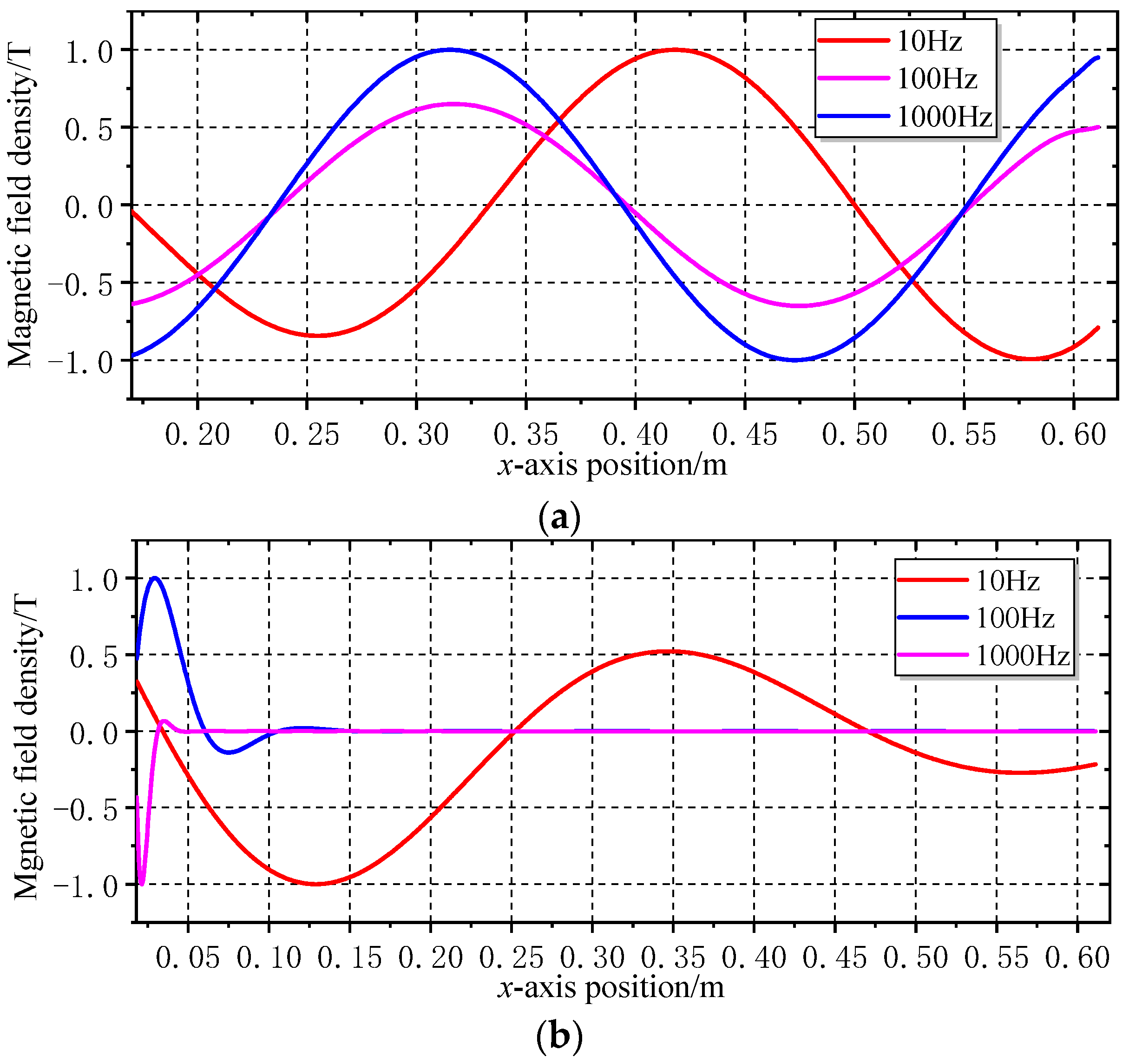
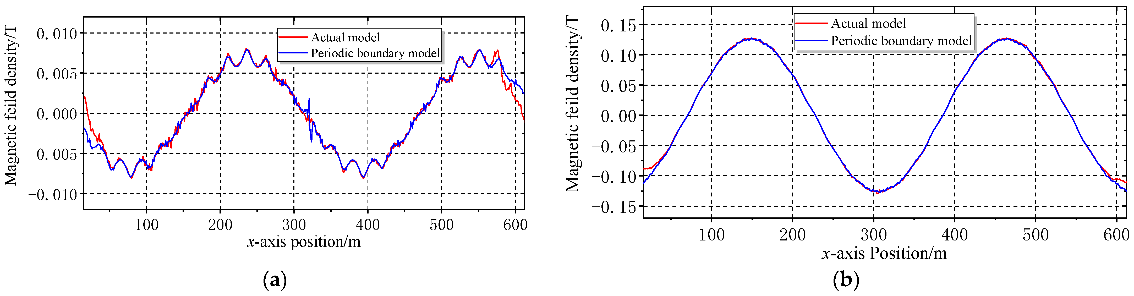
3.2.2. Verification of Analysis Results Based on FEA

To verify the feasibility of utilizing a steady-state field for equivalent calculations of transient fields under high-frequency excitation, the eddy-current periodic boundary FEA models and transient periodic boundary FEA models were established separately. A comparison was made between the spatial magnetic field distributions of the two models under non-periodic transient conditions. The simulation conditions for the transient periodic boundary model were a current amplitude transitioning instantaneously from 0 A to 5000 A within 0 s to 1 s, a current frequency transitioning instantaneously from 4 kHz to 4.02 kHz within 0 s to 1 s, a mover velocity of 4 m/s, and a magnetic field output at the midline of the air gap at 0.5 s. Subsequently, the corresponding current amplitudes and frequencies at 0.5 s were loaded into the eddy-current periodic boundary model, and the magnetic field at the midline of the air gap was output. The output results of the two models were compared, as shown in Figure 11.

From the comparison results, it can be observed that the y-direction and x-direction MFs exhibit good agreement between the eddy-current and transient models, which implies that under high-frequency excitation, the transient field at each moment closely approximates the eddy-current field. Therefore, under high-frequency excitation, it is feasible to employ the steady-state (eddy-current) field for equivalent calculations of the transient field.

4. Novel Simplified Modeling of High-Frequency Electromagnetic Forces in LIMs

4.1. Establishment of High-Frequency MF Analytical Model for LIM

4.1.1. Derivation of Theoretical Formulas

Based on the above analysis, the computational challenge of high-frequency MFs during transient operation can be simplified to the calculation under steady-state conditions with periodic boundaries. So, for high-frequency fields, the subdomain method can be used.

Due to the y-direction and x-direction magnetic field distribution differences in the air gap of the LIM under PWM current excitation, a 2D electromagnetic field subdomain model was established to compute the y-direction and x-direction EFs on the windings and conductive layers, as shown in Figure 12.

To simplify the expression, a 2D model was established within a Cartesian coordinate system. Subsequently, the three-dimensional characteristics were obtained through the application of axisymmetric relationships.

The model was divided into three subdomains: the primary current layer (Subdomain 1), the air gap layer (Subdomain 2), and the secondary conductive layer (Subdomain 3). To streamline the computation, the following assumptions were made:

• The currents on the primary current layer and secondary conductive layer have only the z-axis component;
• The primary moves in the positive x-axis direction;
• All field quantities vary sinusoidally with time;
• The magnetic permeability of the primary and secondary cores is infinite.

Derived from the Maxwell equation set, the governing equations satisfied by each subdomain are expressed as

$${\displaystyle \frac{{\partial }^2{A}_{\mathrm{z}i}}{\partial x^2}}+{\displaystyle \frac{{\partial }^2{A}_{\mathrm{z}i}}{\partial y^2}}={\mu }_i{\sigma }_i\left({\displaystyle \frac{\partial A_{\mathrm{z}i}}{\partial t}}+V{\displaystyle \frac{\partial A_{\mathrm{z}i}}{\partial x}}\right)$$

(10)

where A_zi represents the vector magnetic potential of subdomain i, as expressed in (11), where v corresponds to the harmonic order.

$$A_{\mathrm{z}i}=A_i\left(y\right)e^{j(\omega t-v\beta x)}$$

(11)

Simplifying the governing equations based on the characteristics of each subdomain, the governing equation for Subdomain 1 can be reduced to (12).

$${\displaystyle \frac{{\partial }^2{A}_{\mathrm{z}1}}{\partial x^2}}+{\displaystyle \frac{{\partial }^2{A}_{\mathrm{z}1}}{\partial y^2}}={\mu }_0{J}_{v\mathrm{z}1}$$

(12)

where J_vz1 represents the current distribution density on the primary current layer plane. Its expression is given by (13).

$$J_{\mathrm{z}v1}={\displaystyle \frac{m_{\mathrm{p}}N{K}_{\mathrm{w}\mathrm{v}}{I}_v}{P\tau h_{\mathrm{c}\mathrm{o}}}}{e}^{j(\omega t-v\beta x)}$$

(13)

where m_p denotes the number of motor phases, N represents the number of turns in the winding, K_wv is the winding distribution coefficient, and I_v is the amplitude of the vth harmonic current.

In Subdomain 2, where the conductivity is 0, the governing equation can be simplified to (14).

$${\displaystyle \frac{{\partial }^2{A}_{\mathrm{z}2}}{\partial x^2}}+{\displaystyle \frac{{\partial }^2{A}_{\mathrm{z}2}}{\partial y^2}}=0$$

(14)

In Subdomain 3, expanding the partial derivatives in (10) yields (15) and (16).

$${\displaystyle \frac{\partial A_{\mathrm{z}3}}{\partial t}}=j\omega A_3(y){\mathrm{e}}^{j(\omega t-v\beta x)}$$

(15)

$${\displaystyle \frac{\partial A_{\mathrm{z}3}}{\partial x}}=-jV\beta A_3(y){\mathrm{e}}^{j(\omega t-v\beta x)}$$

(16)

Due to the fact that the PWM current frequency ω is significantly greater than the mover motion velocity V, (15) dominates (16) by a large margin. When solving the governing equation for Subdomain 3, (16) can be safely neglected, effectively assuming the velocity V to be 0. Finaly, the governing equation for Subdomain 3 can be simplified to the following form:

$${\displaystyle \frac{{\partial }^2{A}_{\mathrm{z}3}}{\partial x^2}}+{\displaystyle \frac{{\partial }^2{A}_{\mathrm{z}3}}{\partial y^2}}={\mu }_0{\sigma }_3{\displaystyle \frac{\partial A_{\mathrm{z}3}}{\partial t}}$$

(17)

Solving differential Equations (12), (14), and (17) leads to the general solution for the magnetic potential A_zi in each subdomain:

Subdomain 1:

$$A_{\mathrm{z}1}(y)=C_1{e}^{v\beta y}+{C_1}^{\prime }{e}^{-v\beta y}-{\displaystyle \frac{{\mu }_0{J}_{\mathrm{z}v1}}{v^2{\beta }^2}}$$

(18)

Subdomain 2:

$$A_{\mathrm{z}2}(y)=C_2{e}^{v\beta y}+{C_2}^{\prime }{e}^{-v\beta y}$$

(19)

Subdomain 3:

$$A_{\mathrm{z}3}(y)=C_3{e}^{ry}+{C_3}^{\prime }{e}^{-ry}$$

(20)

$$r=\sqrt{j\omega {\mu }_0{\sigma }_3+v^2{\beta }^2}$$

(21)

The boundary conditions at the interfaces between each subdomain are as follows, where B_xi represents the MF density in the x-direction within subdomain i, and B_yi represents the MF density in the y-direction within subdomain i.

• When y = 0, B_x1 = 0;
• When y = h_co, B_x1 = B_x2, B_y1 = B_y2;
• When y = h_co + g_e, B_x2 = B_x3, B_y2 = B_y3;
• When y = h_co + g_e + h_cl, B_x3 = 0.

By employing the general solution for the magnetic potential A_zi in each subdomain and considering the boundary conditions, six sets of linear equations can be derived. These six sets of linear equations are simultaneously solved and yield the numerical values C₁, C′₁, C₂, C′₂, C₃, and C′₃. Subsequently, the magnetic field equations for subdomains 1, 2, and 3, as well as the eddy-current equation for subdomain 3, can be obtained. The specific forms of these equations are as follows.

MF equation of subdomain 1:

$$B_{\mathrm{x}1}(x,y)=\left(v\beta C_1{e}^{v\beta y}-v\beta C_1^{\prime }{e}^{-v\beta y}\right)e^{j(\omega t-v\beta x)}$$

(22)

$$B_{\mathrm{y}1}(x,y)=j\beta k\left(\begin{array}{l}{C}_1{e}^{v\beta y}+C_1^{\prime }{e}^{-v\beta y}\\ -{\displaystyle \frac{{\mu }_0{J}_{\mathrm{z}v1}}{v^2{\beta }^2}}\end{array}\right)e^{j(\omega t-v\beta x)}$$

(23)

MF equation of subdomain 2:

$$B_{\mathrm{x}2}(x,y)=\left(v\beta C_2{e}^{v\beta y}-v\beta C_2^{\prime }{e}^{-v\beta y}\right)e^{j(\omega t-v\beta x)}$$

(24)

$$B_{\mathrm{y}2}(x,y)=jv\beta \left(C_2{e}^{\beta ky}+C_2^{\prime }{e}^{-\beta ky}\right)e^{j(\omega t-v\beta x)}$$

(25)

MF equation and eddy-current equation of subdomain 3:

$$B_{\mathrm{x}3}(x,y)=\left(r{C}_3{e}^{ry}-r{C}_3^{\prime }{e}^{-ry}\right)e^{j(\omega t-v\beta x)}$$

(26)

$$B_{\mathrm{y}3}(x,y)=jv\beta \left(C_3{e}^{ry}+C_3^{\prime }{e}^{-ry}\right)e^{j(\omega t-v\beta x)}$$

(27)

$$J_{\mathrm{z}v3}(x,y)=j\omega {\sigma }_3\left(C_3{e}^{ry}+C_3^{\prime }{e}^{-ry}\right)e^{j(\omega t-v\beta x)}$$

(28)

The MF excited by each harmonic current can be superimposed according to the magnetic field superposition theorem.

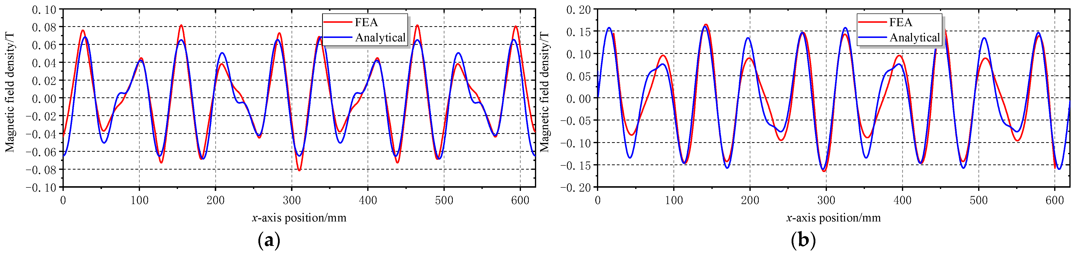
4.1.2. Validated by FEA

To validate the accuracy of the 2D subdomain model, a periodic boundary eddy-current FEA model was established for comparison.

The simulation input of the FEA model comprised harmonic currents derived from the inverter output. The inverter operated at a switching frequency of 4 kHz and a fundamental frequency of 10 Hz. Subsequently, the current with a frequency of 4020 Hz was extracted from the harmonic components of the inverter current. Then, these currents were utilized as excitation inputs for the FEA model and analytical model.

A comparative analysis was performed between the analytical and FEA models for the air gap magnetic field; the comparative results are presented in Figure 13.

We extracted the current with a frequency of 8010 Hz from the harmonic components of the inverter current, serving as the excitation for the FEA model and analytic model. The comparative results are illustrated in Figure 14.

From Figure 13 and Figure 14, it can be observed that the FEA simulation results are in good agreement with the analytical calculations. Given the modulation strategy employed in this experiment, which involves carrier phase shifting by 90 degrees, the primary harmonic orders in the air gap magnetic field are 11th and 13th in the vicinity of frequency fc ± 2fr, while at frequency 2fc ± fr (fc represents the switching frequency, and fr represents the fundamental frequency), the dominant harmonic orders are 5th and 7th. Hence, the magnetic field waveforms differ at frequencies of 4020 Hz and 8010 Hz.

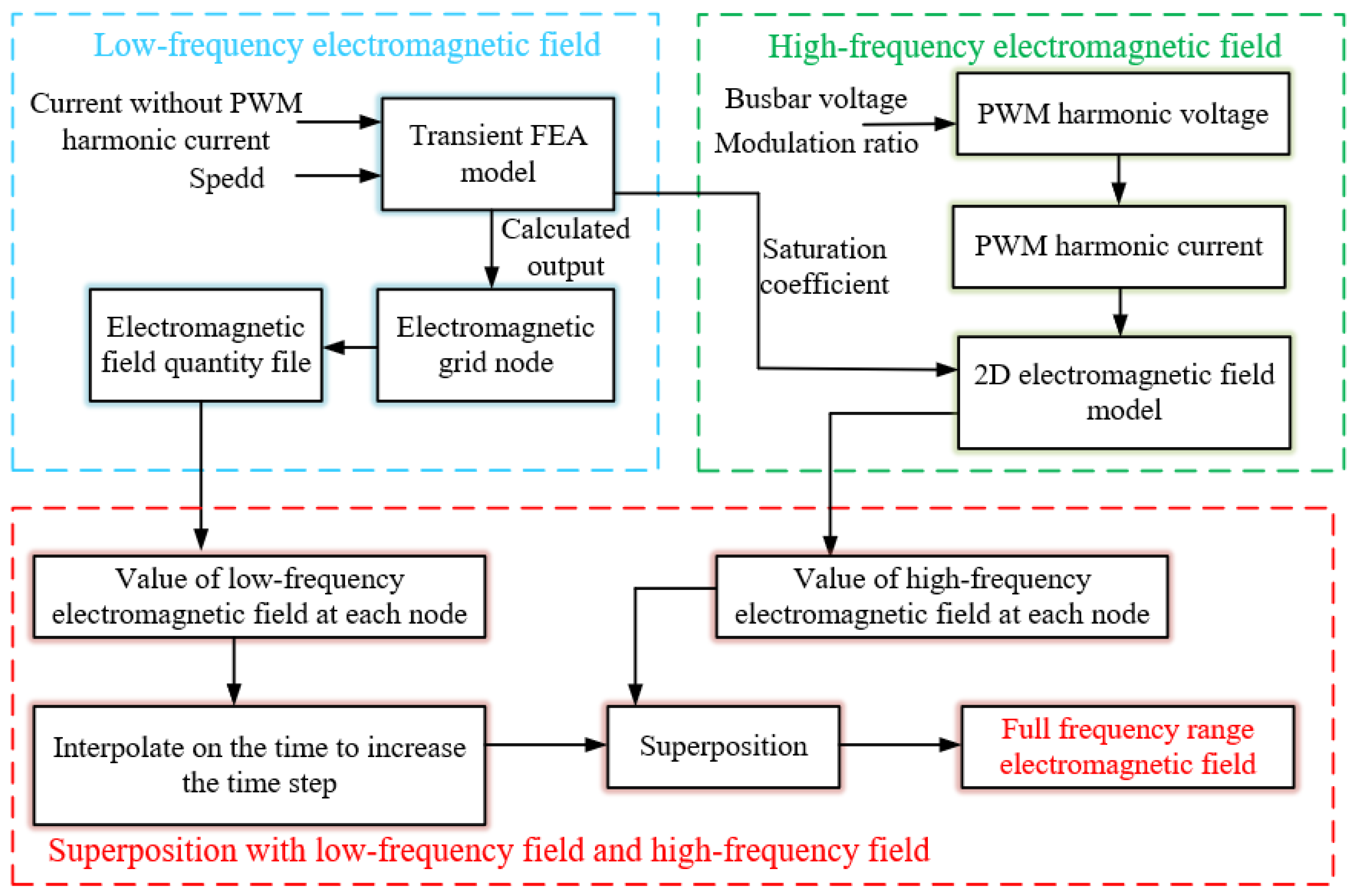
4.2. Calculation Flow of MF Model

This section introduces a rapid computational method for the transient MF calculation of LIM, combining low-frequency FEA transient field calculations with high-frequency analytical computations. The computational workflow is illustrated in Figure 15. For low-frequency electromagnetic field calculations, FEA is performed using Ansys Maxwell software (2022R1) for modeling. For high-frequency electromagnetic field calculations, MATLAB (2021A) is utilized for programmatic modeling.

The computational process comprises three components: low-frequency electromagnetic field calculation, high-frequency electromagnetic field calculation, and magnetic field superposition. For low-frequency electromagnetic field analysis under transient operating conditions, an FEA model is employed due to the complex time-varying MF variations within LIMs, which cannot be adequately described by analytical models. This module takes current and mover velocity as inputs, outputting time-step field data including mesh information and field quantities. The high-frequency electromagnetic field calculation integrates a three-phase full-bridge inverter output voltage analytical model with our proposed high-frequency electromagnetic field model. The inverter voltage model is derived through double Fourier decomposition, retaining only switching frequency-related harmonic currents and their multiples by filtering low-frequency components. Subsequent field quantities across subdomains are computed using the high-frequency analytical model. As low-frequency field data are discrete while high-frequency results are continuous, node coordinates are utilized to convert continuous high-frequency field quantities into discrete data prior to superposition with their low-frequency counterparts. The complete workflow proceeds as follows:

Initially, the MF calculations are divided into low-frequency and high-frequency components, which can be performed simultaneously. For low-frequency MF calculations, it is imperative to establish a transient FEA model. The fundamental current and mover velocity profiles are sent into the transient FEA model, which computes the electromagnetic field quantities at each node for every moment and outputs of the results as data files. Due to the large amplitude of the fundamental wave current, core saturation occurs, while the smaller amplitude of the high-frequency currents contributes less to saturation. Therefore, the saturation state of the core in the low-frequency MF can be applied to the high-frequency MF. The saturation coefficient k_s is defined by the output of the low-frequency electromagnetic field at each moment, as in (29), where B represents the MF considering the nonlinearity of the core, while B₀ represents the MF without considering the nonlinearity of the core.

$$k_{\mathrm{s}}={\displaystyle \frac{B}{B_0}}$$

(29)

Secondly, the PWM currents are then computed using an equivalent port model [31] and incorporated into the 2D analytic model developed in this paper to calculate the high-frequency MF. The MF is then multiplied by the saturation coefficient corresponding to the specific time point, and then, the results are stored accordingly.

Finally, the field quantities of each node in the low-frequency MF are first subjected to temporal interpolation, which increases the sampling rate of low-frequency field data. The sampling rate, in accordance with the sampling theorem, should be higher than or equal to twice the highest frequency of the high-frequency magnetic field. Then, the low-frequency MF quantities are superimposed with the high-frequency electromagnetic field quantities at grid nodes, resulting in the completion of node quantities across the whole frequency spectrum.

To further clarify the distinctions between the proposed method and existing approaches, and to highlight the advantages of the proposed method in calculating high-frequency EFs during the transient operation of LIMs, a comparative analysis between the proposed method and those reported in prior studies is presented in

Table 2. Comparison of the methodology of this paper with that of the relevant literature.

Reference	Suitable for Linear Motors?	Suitable for Transient Conditions?	Suitable for High-Frequency EF Calculation?	Ability to Calculate All Components	Calculation Speed
[7]	√	×	√	×	fast
[32]	√	×	√	×	fast
[33]	√	×	√	×	fast
[34]	×	√	√	×	fast
[35]	√	×	√	×	fast
[36]	√	√	√	√	slow
[37]	√	√	√	√	slow
This paper	√	√	√	√	fast

.

References [7,32,33,34,35] primarily employ analytical methods, calculating the air gap flux density first and subsequently applying Maxwell’s tensor method to determine the EFs at the stator tooth tips. While this approach benefits from rapid computation speed, its air gap flux density formulas are derived under steady-state assumptions, rendering it inapplicable to transient scenarios and incapable for computing EFs on other motor components. In contrast, References [36,37] adopt FEA, which fully satisfy the requirements for high-frequency EF calculations for linear motors in transient operating conditions. However, FEA suffers from slow computation speeds and significant computational resource demands. Our comparative analysis reveals that the proposed method demonstrates notable advantages in high-frequency EF calculations under transient conditions, particularly suited for linear motors operating in non-periodic transient regimes where conventional methods fall short.

4.3. EF Calculation Formula

For the surface of ferromagnetic materials, calculations can be performed using a simplified Maxwell tensor, the expression of which is as follows:

$$F_n={\displaystyle \frac{B_n^2}{2{\mu }_0}}$$

(30)

Here, B_n represents the normal MF density on the surface of the ferromagnetic material. For the conductor components, such as windings and secondary conductive layers, we can use (31).

$$\mathit{f}=\mathit{J}\times \mathit{B}$$

(31)

The main force-bearing components in the LIM include the surface of the primary core (near the winding end face) and the secondary iron core, the primary winding, and the secondary conductive layer. Because the high-frequency MF does not travel through the secondary iron core, high-frequency EFs are not generated on the surface or within the interior of the secondary iron core. Furthermore, as the secondary iron core adopts a laminated structure, it is incapable of generating eddy currents. Therefore, the secondary iron core mainly experiences fundamental EFs on its surface, which are generated by the action of the fundamental magnetic field.

5. Experimental Validation

Since it is challenging to directly measure EFs with testing devices. To validate the results of transient EF calculations, mechanical dynamic FEA methods are typically used to calculate electromagnetic vibration responses and compare them to experimental vibration test results. It is worth stating that this experiment was constructed to verify that the model was correct.

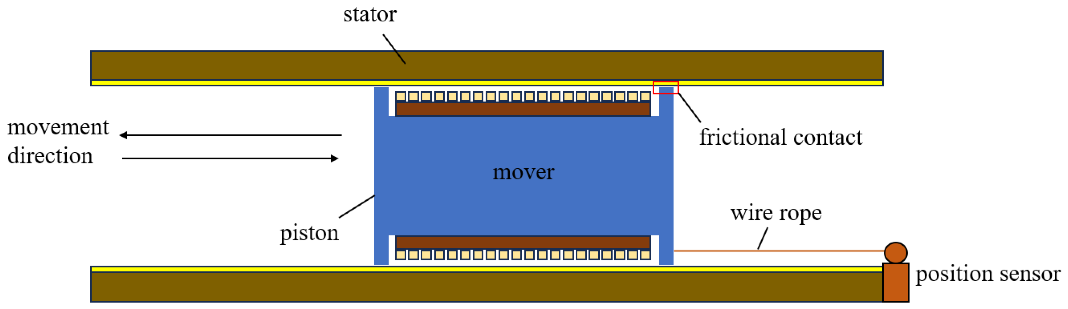
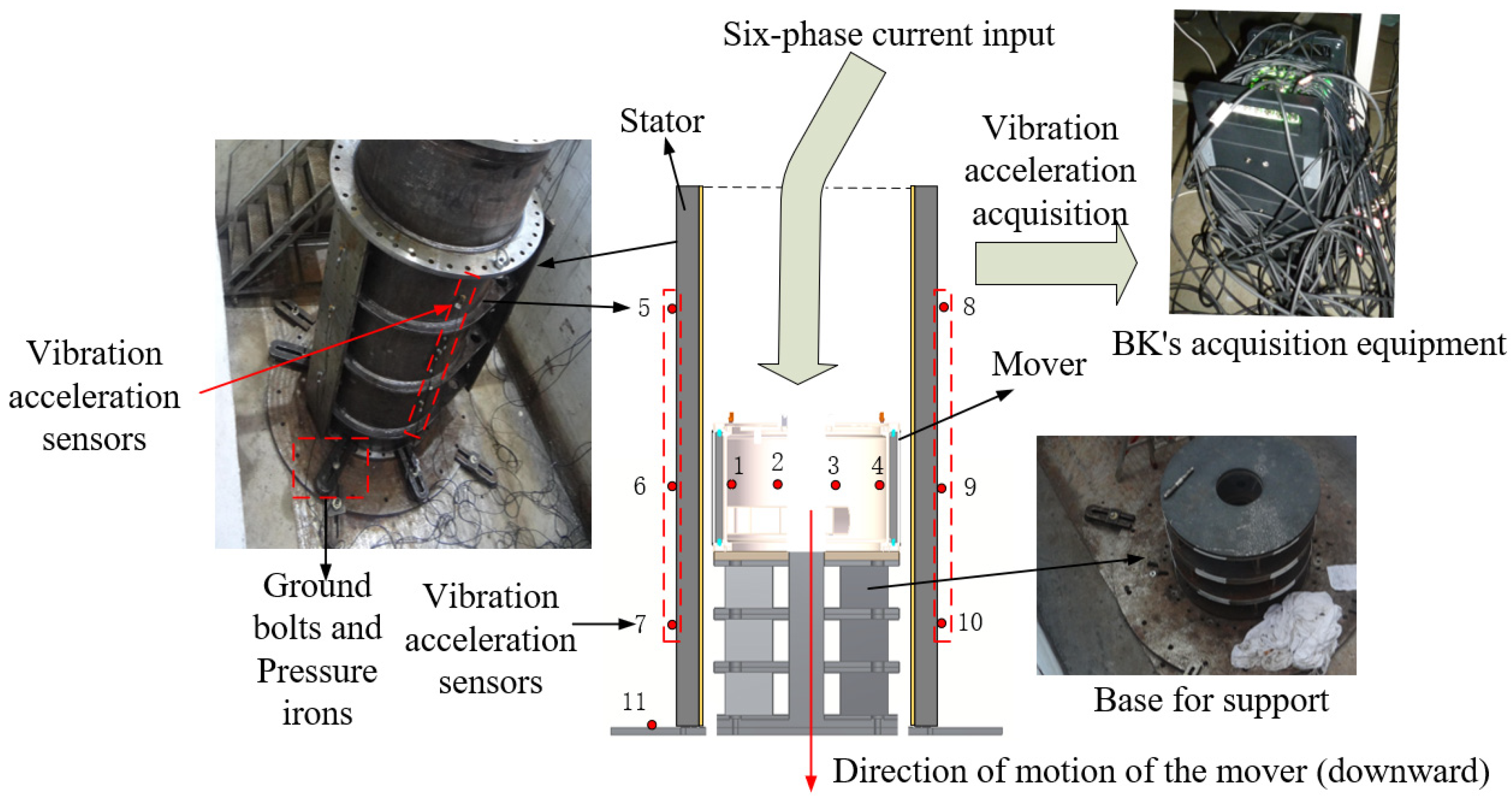
5.1. Experimental Platform

The subject of this experiment was a cylindrical LIM. Initially, the cylindrical LIM was positioned vertically fastened to the ground using ground anchor bolts and pressure plates. The mover was placed flat on three supporting bases, each measuring around 200 mm in height. If a change in the mover’s position was required, this was achieved by altering the number of overlapping support bases. The experimental platform is shown in Figure 16.

Both the stator and the mover were vertically oriented. This configuration was implemented to prevent a contact relationship between the stator and mover induced by gravity, thereby mitigating the transmission of vibrations between the mover and stator. The mover was elevated to approximately the height of the stator center (600 mm) using overlapping support bases. Its bottom surface was supported by rubber pads arranged on the overlapping support bases, which reduced vibration transfer from the mover to the support base. Simultaneously, this configuration also countered the electromagnetic downward force exerted on the mover during electrical energization. The bottom surface of the stator was bolted to the base to imitate a permanent link to the ground, thereby counteracting the vertical electromagnetic upward force experienced by the stator. The experiment employed 11 uniaxial acceleration sensors, which were mounted on the outer surface of the stator and foot, with signal lines connecting them to a multi-channel data acquisition device.

The stator was fixed to the ground, and considering the substantial stiffness of the ground, the vibrations of the stator were effectively isolated from the ground. Similarly, the supporting base was also fixed to the ground, with a 2 mm gap between its inner wall and the stator, preventing the vibrations of the mover from transmitting to the ground while also isolating the stator.

According to the analysis, there was no vibration transmission channel between the mover and the stator under these experimental conditions. Therefore, in establishing the mechanical dynamic FEA model, the stator and the mover could be modeled separately, with EFs applied individually to compute their respective vibration responses.

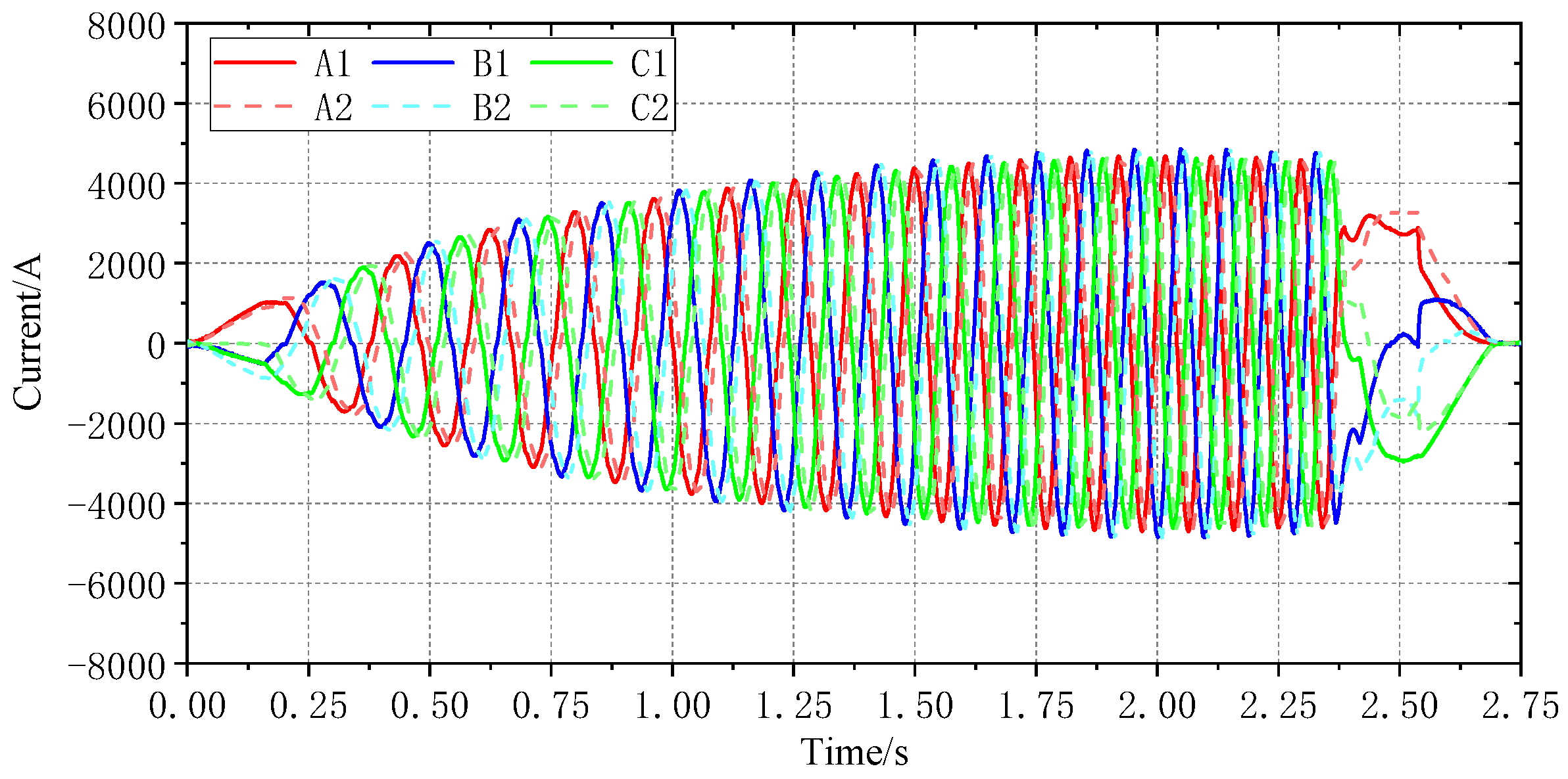
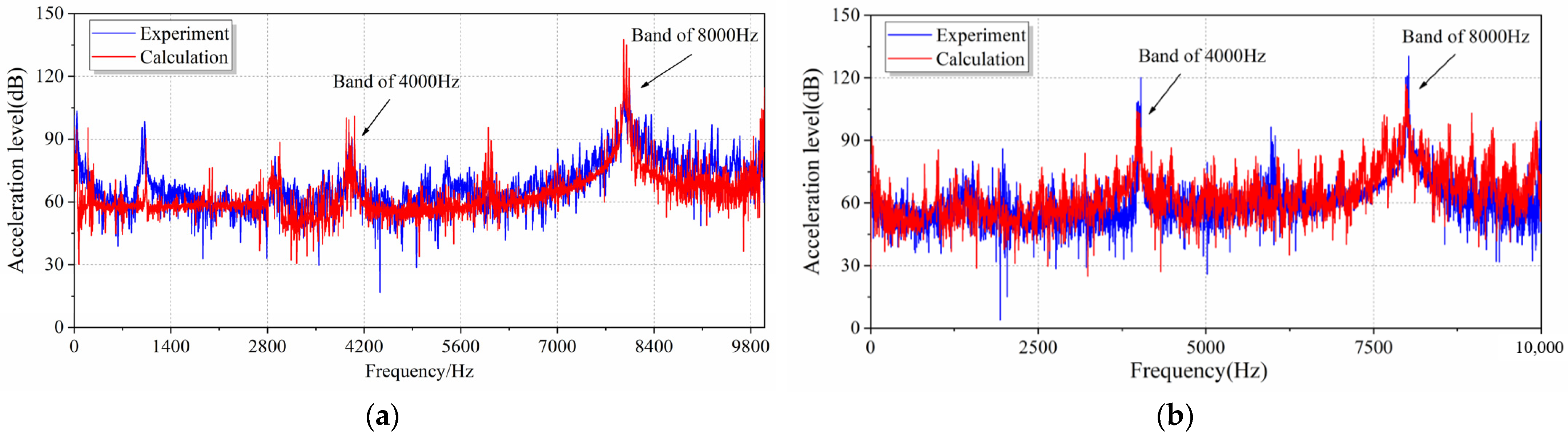
5.2. Experimental Validation Results

Establishing the mechanical dynamic FEA model, the stator and the mover could be modeled separately, with EFs applied individually to compute their respective vibration responses.

In the preliminary phase, we completed the dynamical modeling, and details of the study process can be found in [38,39]. Based on the research foundation of the LIM dynamic model in [38], the EFs calculated using the method in this paper were applied to the dynamic models of the stator and mover, and their vibration responses were calculated. The method of validating the analytical model through experimentation is shown in Figure 17.

The experimental conditions employed for validation were as follows: a peak current of 5000 A, a supply frequency ranging from 0 Hz to 12 Hz, and a switching frequency of 4 kHz. The current waveform is shown in Figure 18.

We Utilized the experimentally derived operational conditions to compute the EF acting on the stator and mover with the EF calculation model. Subsequently, based on the coordinates of the mesh nodes in the dynamic FEA model, the computed EF excitations were applied. Finally, the vibrational response generated by the mechanical dynamic model was computed, and the corresponding vibration acceleration data at designated measurement points was outputted.

Figure 19 displays a comparative analysis between the calculation and experimental results for vibration accelerations at measurement points, encompassing acceleration magnitudes and velocity spectra within the 10 kHz range.

Our research team conducted FEA modeling, model analysis, vibration testing, and model calibration of the LIM dynamic model in the earlier stages, ensuring the correctness of the dynamic model used in this paper.

Examining the vibration acceleration spectrum throughout the whole frequency range reveals that the calculated results are perfectly consistent with the experimental data, indirectly confirming the accuracy of the EF calculation model. From the comparison, it can be observed that the vibrations at the switching frequency and its harmonic bands are the most significant, constituting the primary vibrations. Further analysis of the vibration results can be found in References [38,39].

6. Conclusions

This study analyzes the MF characteristics of a LIM under PWM current excitation. It is concluded that under high-frequency current excitation, the end effect of the LIM is weak. The usage of a periodic boundary model is effective in obtaining an equivalent representation of the actual model. Furthermore, the transient processes are extremely short under high-frequency current excitation, allowing the transformation of transient calculation to be converted into steady-state calculation.

Based on these two crucial conclusions, a rapid transient high-frequency EF calculation method optimized for LIMs is proposed. This method represents a hybrid approach combining FEA and analytical methodologies. Specifically, the low-frequency MF is computed using transient FEA, while the high-frequency MF is evaluated through analytical models. Subsequently, the complete field quantity data for each node are obtained by employing the principle of MF superposition.

Finally, the computed EF loads are applied to the dynamic model of the LIM to calculate the vibration response. Then, vibration test are conducted to confirm the correctness of the EF calculations.

This method, compared to FEA, enables the rapid and accurate calculation of transient high-frequency EFs, making it suitable for application in the iterative stages of motor optimization design and applicable to rotary induction motors.

References

1. Zhang, Q.; Zhang, Y. Scheme design of high performance converting control of linear induction motor used for electromagnetic launch. In Proceedings of the 16th International Symposium on Electromagnetic Launch Technology (EML), Beijing, China, 15–19 May 2012. [Google Scholar]
2. Zhang, Y.; Zhang, M.; Ma, W.; Xu, J.; Lu, J.; Sun, S. Modeling of a double-stator linear induction motor. IEEE Trans. Energy Convers. 2012, 27, 572–579. [Google Scholar] [CrossRef]
3. Schnegas, M.; Jouaneh, M.K. Trajectory Planning for Reciprocating Motion in Integrated Servo Motor Linear Stages. Machnies 2024, 12, 934. [Google Scholar] [CrossRef]
4. Yoon, D.S.; Choi, S.B. Adaptive Control for Suspension System of In-Wheel Motor Vehicle with Magnetorheological Damper. Machnies 2024, 17, 433. [Google Scholar] [CrossRef]
5. Hoshina, T.; Yamada, T.; Deng, M. Perfect Tracking Control of Linear Sliders Using Sliding Mode Control with Uncertainty Estimation Mechanism. Machnies 2024, 12, 212. [Google Scholar] [CrossRef]
6. Ding, A.; Huang, C.; Sun, Z.; Zeng, R.; Mao, Y.; Jia, G. Six-phase cylindrical linear induction motor with high-frequency vibration suppression and experimental study. In Proceedings of the IEEE 5th International Electrical and Energy Conference (CIEEC), Nangjing, China, 27–29 May 2022. [Google Scholar]
7. Ji, Z.; Cheng, S.; Li, X.; Lv, Y.; Wang, D. An Optimal Periodic Carrier Frequency PWM Scheme for Suppressing High-Frequency Vibrations of Permanent Magnet Synchronous Motors. IEEE Trans. Power Electron. 2023, 38, 13008–13018. [Google Scholar] [CrossRef]
8. Liu, Z.; Yan, S.; Fang, H.; Jiang, D.; Qu, R.; Wang, Q. Research on High Frequency Vibration Reduction Using Carrier Phase Shifted PWM for 4-Module 3-Phase Permanent Magnet Synchronous Motor. IEEE Trans. Ind. Appl. 2022, 58, 7192–7200. [Google Scholar] [CrossRef]
9. Han, Z.; Xu, J.; Rui, W.; Zhang, Y.; Li, M. Research on Thrust Ripple of Aperiodic Transient Linear Induction Motors. In Proceedings of the 13th International Symposium on Linear Drives for Industry Applications (LDIA), Wuhan, China, 1–3 July 2021. [Google Scholar]
10. Han, Z.; Xu, J.; Rui, W.; Wang, L.; Li, G. Analysis of Electromagnetic Force of Linear Induction Motor with Segmented Power Supply for Electromagnetic Emission. In Proceedings of the 2020 Asia Energy and Electrical Engineering Symposium (AEEES), Chengdu, China, 29–31 May 2020. [Google Scholar]
11. Chen, M.; Deng, J.; Yang, Y.; Zhou, H.; Tao, T.; Liu, S.; Hua, L. Performance analysis of a floating wind–wave power generation platform based on the frequency domain model. J. Mar. Sci. Eng. 2024, 12, 206. [Google Scholar] [CrossRef]
12. Wang, J.; Chen, Z.; Zhang, F. A review of the optimization design and control for ocean wave power generation systems. Energies 2021, 15, 102. [Google Scholar] [CrossRef]
13. Ahamed, R.; McKee, K.; Howard, I. A review of the linear generator type of wave energy converters’ power take-off systems. Sustainability 2022, 14, 9936. [Google Scholar] [CrossRef]
14. Curto, D.; Franzitta, V.; Guercio, A.; Miceli, R.; Nevoloso, C.; Raimondi, F.M.; Trapanese, M. An experimental comparison between an ironless and a traditional permanent magnet linear generator for wave energy conversion. Energies 2022, 15, 2387. [Google Scholar] [CrossRef]
15. Epifanov, A.P.; Kril, D.B. Linear asynchronous electric drive of the monorail transport system for feeding in livestock farms. Izv. St.-Petersburg State Agrar. Univ. 2022, 66, 113–124. [Google Scholar]
16. Palka, R.; Woronowicz, K. Linear induction motors in transportation systems. Energies 2021, 14, 2549. [Google Scholar] [CrossRef]
17. Prasad, N.; Jain, S. Linear Motor-Based High-Speed Rail Transit System: A Sustainable Approach. Transportation Energy and Dynamics; Singapore: Springer Nature Singapore, 2023; pp. 87–127. [Google Scholar]
18. Fironov, A.N.; Kostenko, A.S. Dynamic model of the Moscow monorail transport system using magnetolevitation technology. Mod. Transp. Syst. Technol. 2022, 8, 67–85. [Google Scholar] [CrossRef]
19. Abdo, M.M.M.; El-Hussieny, H.; Miyashita, T.; Ahmed, S.M. Design of a new electromagnetic launcher based on the magnetic reluctance control for the propulsion of aircraft-mounted microsatellites. Appl. Syst. Innov. 2023, 6, 81. [Google Scholar] [CrossRef]
20. Chi, S.; Yan, J.; Guo, J.; Zhang, Y. Analysis of mechanical stress and vibration reduction of high-speed linear motors for electromagnetic launch system. IEEE Trans. Ind. Appl. 2022, 58, 7226–7240. [Google Scholar] [CrossRef]
21. Ji, Z.; Cheng, S.; Ren, Q.; Li, X.; Lv, Y.; Wang, D. The Effects and Mechanisms of Periodic-Carrier-Frequency PWM on Vibrations of Multiphase Permanent Magnet Synchronous Motors. IEEE Trans. Power Electron. 2023, 38, 8696–8706. [Google Scholar] [CrossRef]
22. Li, J.; Tong, W.; Wu, S. Analytical Model for No-Load Rotor Bracket Loss of Axial flux Hybrid Excitation Motor based on Subdomain Method. In Proceedings of the 2023 IEEE 6th Student Conference on Electric Machines and Systems (SCEMS), Huzhou, China, 7–9 December 2023. [Google Scholar]
23. Tiang, T.L.; Ishak, D.; Lim, C.P.; Jamil, M.K.M. A Comprehensive Analytical Subdomain Model and Its Field Solutions for Surface-Mounted Permanent Magnet Machines. IEEE Trans. Magn. 2015, 51, 8104314. [Google Scholar] [CrossRef]
24. Golovanov, D.; Galassini, A.; Transi, T.; Gerada, C. Analytical Methodology for Eddy Current Loss Simulation in Armature Windings of Synchronous Electrical Machines with Permanent Magnets. IEEE Trans. Ind. Electron. 2022, 69, 9761–9770. [Google Scholar] [CrossRef]
25. Gu, L.; Bostanci, E.; Moallem, M.; Wang, S.; Devendra, P. Analytical calculation of the electromagnetic field in SRM using conformal mapping method. In Proceedings of the 2016 IEEE Transportation Electrification Conference and Expo (ITEC), Dearborn, MI, USA, 27–29 June 2016. [Google Scholar]
26. Dong, K.; Yu, H.; Hu, M.; Liu, J.; Huang, L.; Zhou, J. Study of Axial-Flux-Type Superconducting Eddy-Current Couplings. IEEE TAS 2017, 27, 0600905. [Google Scholar] [CrossRef]
27. Yamazaki, K.; Kuramochi, S.; Fukushima, N.; Yamada, S.; Tada, S. Characteristics Analysis of Large High Speed Induction Motors Using 3-D Finite Element Method. IEEE Trans. Magn. 2012, 48, 995–998. [Google Scholar] [CrossRef]
28. Liang, Y.; Bian, X.; Yu, H.; Li, C. Finite-Element Evaluation and Eddy-Current Loss Decrease in Stator End Metallic Parts of a Large Double-Canned Induction Motor. IEEE Trans. Ind. Electron. 2015, 62, 6779–6785. [Google Scholar] [CrossRef]
29. Seno, R.; Manabe, T.; Matsutomo, S.; Hidaka, Y. Interactive Motor Design System Using 2-D Finite Element Analysis With Fast Mesh Modification Method. IEEE Trans. Magn. 2022, 58, 7401004. [Google Scholar] [CrossRef]
30. Nasar, S.A.; Del Cid, L. Certain approaches to the analysis of single-sided linear induction motors. IEE Proc. 1973, 120, 477–483. [Google Scholar] [CrossRef]
31. Li, M.; Xu, J.; Zhang, Y.Z.P.; Han, Z. Calculation and Analysis of PWM Harmonic Current of Multiphase Linear Induction Motor. J. Nav. Univ. Eng. 2024, 36, 105–112. [Google Scholar]
32. Ma, C.; Wang, Y.; Chen, H.; Hong, J.; Wang, Y. Analysis of Electromagnetic Vibration in Permanent Magnet Motors Based on Random PWM Technology. Machines 2025, 13, 259. [Google Scholar] [CrossRef]
33. Casisa, A.; Lafarge, B.; Lanfranchi, V. Investigations of Vibratory Lines from PWM in Order to Recover Vibratory Energy on an Electric Machine. In Proceedings of the 2024 IEEE International Conference on Industrial Technology (ICIT), Bristol, UK, 25–27 March 2024. [Google Scholar]
34. Fan, L.; Liu, Z.; Jiang, D.; Qu, R. Research on High-Frequency Vibration Reduction for Active Magnetic Bearings with Carrier Phase Shifting PWM. IEEE Trans. Ind. Electron. 2025, 72, 5527–5537. [Google Scholar] [CrossRef]
35. Lv, Y.; Cheng, S.; Ji, Z.; Li, X.; Wang, D.; Wei, Y. Spatial-Harmonic Modeling and Analysis of High-Frequency Electromagnetic Vibrations of Multiphase Surface Permanent-Magnet Motors. IEEE Trans. Ind. Electron. 2023, 70, 11865–11875. [Google Scholar] [CrossRef]
36. Yan, R.; Wang, D.; Wang, C.; Miao, W.; Wang, X. Analytical Approach and Experimental Validation of Sideband Electromagnetic Vibration and Noise in PMSM Drive with Voltage-Source Inverter by SVPWM Technique. IEEE Trans. Magn. 2025, 61, 8200206. [Google Scholar] [CrossRef]
37. Kim, J.H.; Won, Y.J.; Lim, M.S. Analysis and Reduction of Radial Vibration of FSCW PMSM Considering the Phase of Radial, Tangential Forces, and Tooth Modulation Effect. IEEE Trans. Transp. Electrif. 2025, 11, 2976–2987. [Google Scholar] [CrossRef]
38. Zhang, Y.; Xu, J.; Li, M.; Yu, A.; Wu, D. Modelling and analysis of electromagnetic vibration in long sheet secondary tubular linear induction motors. IET Electr. Power Appl. 2023, 17, 1237–1366. [Google Scholar] [CrossRef]
39. Guo, G.; Zhao, Y.; Yu, A. Analysis of electromagnetic vibration of submerged tubular linear motors based on wave propagation approach. Wave Motion 2024, 127, 103287. [Google Scholar] [CrossRef]
Figure 1. Research methodology and approach.
Machines 13 00409 g001
Figure 2. Inverter of double three-phase LIM.
Machines 13 00409 g002
Figure 3. Structure of the double three-phase LIM.
Machines 13 00409 g003
Figure 4. Mechanism and motion process of LIM.
Machines 13 00409 g004
Figure 5. Zeros-point distribution.
Machines 13 00409 g005
Figure 6. Air gap MF at supply frequencies of 10 Hz, 100 Hz, and 1000 Hz. (a) Total air gap MF; (b) Inlet wave MF; (c) Outlet wave MF.
Machines 13 00409 g006aMachines 13 00409 g006b
Figure 7. FEA models for the actual structure and periodic boundary structure.
Machines 13 00409 g007
Figure 8. Comparison of the y-direction and x-direction MF densities between the actual model and the periodic boundary model at 0.3 s. (a) A comparison of MFs in the y-direction; (b) a comparison of MFs in the x-direction.
Machines 13 00409 g008
Figure 9. High-frequency-excitation-induced MF distribution in LIM.
Machines 13 00409 g009
Figure 10. Application of a step magnetic field on the surface of a semi-infinite conductor.
Machines 13 00409 g010
Figure 11. A comparison of magnetic fields at the midline of the electromagnetic air gap between the transient model and the eddy-current model at 0.5 s. (a) MF in y-direction; (b) MF in x-direction.
Machines 13 00409 g011
Figure 12. Periodic boundary 2D subdomain model.
Machines 13 00409 g012
Figure 13. Comparison between FEA and analytical models in frequency band of 4020 Hz. (a) MF in y-direction; (b) MF in x-direction.
Machines 13 00409 g013
Figure 14. Comparison between FEA and analytical models in frequency band of 8010 Hz. (a) MF in y-direction; (b) MF in x-direction.
Machines 13 00409 g014
Figure 15. Transient MF calculation flow for LIM.
Machines 13 00409 g015
Figure 16. Experimental platform for cylindrical LIM.
Machines 13 00409 g016
Figure 17. The method of validating the analytical model through experimentation.
Machines 13 00409 g017
Figure 18. The waveform of the input current.
Machines 13 00409 g018
Figure 19. Comparison between experimental and calculated acceleration results. (a) Measurement point of mover; (b) measurement point of stator.
Machines 13 00409 g019