Improving Vehicle Dynamics: A Fractional-Order PI^λD^μ Control Approach to Active Suspension Systems

Abstract

This paper presents a comprehensive vehicle model featuring an active suspension system integrated with semi-active seat and engine mounting controls. The time-domain stochastic excitation of the four tires was modeled using the filtered white noise method, and the required road excitation was simulated using MATLAB software R2022b. Four comprehensive performance indices, including engine dynamic displacement, vehicle body acceleration, suspension dynamic deflection, and tire dynamic displacement, were selected and made dimensionless by the performance indices of a passive suspension under the same working conditions to construct the fitness function. A fractional-order PI^λD^μ (FOPID) controller was proposed, and its structural parameters were optimized using a gray wolf optimization algorithm. Furthermore, the optimized FOPID controller was evaluated under five road conditions, and its performance was compared with integer-order PID control and passive suspensions. The results demonstrate that the FOPID controller effectively improves the smoothness of the vehicle by reducing engine mounting deflection, vehicle body acceleration, suspension deflection, and tire displacement. Moreover, the simulation results indicate that, compared to the passive suspension, the FOPID-controlled suspension achieves an average optimization of over 42% in the root mean square (RMS) of body acceleration under random road conditions, with an average optimization of more than 38% for suspension deflection, 4.3% for engine mounting deflection, and 2.5% for tire displacement. In comparison to the integer-order PID-controlled suspension, the FOPID-controlled suspension demonstrates an average improvement of 28% in the RMS of acceleration and a 2.1% improvement in suspension deflection under random road conditions. However, the engine mounting deflection and tire displacement are reduced by 0.05% and 0.3%, respectively. FOPID control has better performance in vehicle acceleration control but shows asymmetrical effects on tire dynamic deflection.

1. Introduction

The change in body height of passive suspension during driving depends on the deformation of the spring [1]. Some vehicles use relatively soft springs, which can lead to significant deformation stroke under full load, causing the ground clearance to vary by several tens of millimeters between unloaded and loaded states, affecting the passability of vehicles [2]. Different driving conditions require different suspension settings. Generally, a softer suspension is preferred for comfort during normal driving, while a harder suspension is needed for stability during sharp turns and braking [3]. However, passive suspensions cannot meet these conflicting demands. The increasing trend toward vehicle intelligence, electrification, connectivity, and sharing has created a demand for comprehensive control over vehicle dynamics and full-by-wire chassis systems [4]. The advantages of a full-by-wire chassis, such as rapid response, flexible layout, and electromechanical decoupling, directly support the implementation of vehicle dynamics collaborative control and intelligent driving technologies [5]. With the use of advanced sensors and electronic control systems, full-active suspension systems can adjust the suspension settings at millisecond speeds based on real-time monitoring of road conditions and vehicle status [6]. This technological advancement enhances the driving experience by providing a more precise, flexible ride that optimally balances comfort and handling [7].

The history of automatic control theory can be divided into three main stages: classical control theory, modern control theory, and intelligent control theory [8]. The classical control theory uses transfer functions as mathematical tools and is based on the frequency response method and root locus method [9]. It mainly studies the analysis and design of single input single output systems described by constant coefficient linear differential equations. Common algorithms in classical control theory include proportional-integral-derivative (PID) control [10], root locus design [11], feed-forward control [12], and frequency response design [13]. Modern control theory can not only provide external information (output and input) of the system, but also provide information on internal state variables of the system [14]. It is an effective analysis method for both linear and nonlinear systems, steady-state and time-varying systems, and univariate and multivariate systems. Modern control theory mainly includes optimal control [15], robust control [16], adaptive control [17], sliding mode control [18], model predictive control [19], and Kalman filtering [20]. Intelligent control theory is based on human thinking patterns and problem-solving skills to solve complex control problems that currently require human intelligence [21]. The theory of intelligent control mainly includes fuzzy control [22], neural network control [23], expert control [24], hierarchical intelligent control [25], humanoid intelligent control [26], reinforcement learning control [27], and hybrid intelligent control [28]. The combination of intelligent control and modern control technology is currently an important research direction in the field of automation and control [29]. The combination of intelligent control and modern control techniques allows for the development of more efficient, flexible, and intelligent control systems to cope with the increasingly complex demands of industry and daily life [30]. Intelligent control excels in dealing with systems with uncertain, nonlinear, and complex models, while modern control techniques excel when the system model is clear and precise to improve the robustness of the system to external perturbations and internal parameter variations [31]. In addition, the use of intelligent algorithms to optimize the parameters of modern control systems can further improve system performance on the basis of ensuring system stability and convergence [32]. For example, in fuzzy-PID control combining fuzzy control with classical PID controller, the PID parameters are adjusted by fuzzy logic, so as to realize the adaptive control of the system [33]. In optimal control based on the neural network, neural networks are used to learn the dynamic behavior of the system and optimize the objective function of optimal control theory [34].

In recent years, vehicle technology has been developing toward electrification, intelligence, and networking [35,36]. As a key component of automobiles, the suspension system is also undergoing technological innovation. Research on vehicle suspension is significant in continuously driving the development of the automotive industry, enhancing the competitiveness and market demand of vehicles, and also providing users with a safer and more comfortable driving experience [37,38]. Chen et al. [39] established a PID controller to actively control the suspension, and the controller parameters were adjusted by a fuzzy incremental controller. Simulink verified the effectiveness of the fuzzy incremental controller under different road excitations. Ji et al. [40] proposed an enhanced variable domain fuzzy-PID controller, which was designed by optimizing parameters through an adaptive expansion factor controller and genetic algorithm. Their control strategy can significantly improve vehicle smoothness and reduce the root mean square value of related indicators, providing new ideas for the development of active suspension. Chiou et al. [41] proposed a new design method that utilizes a particle swarm optimization (PSO) reinforcement evolutionary algorithm to determine the optimal fuzzy-PID controller parameters for automotive active suspension systems. Wang et al. [42] established a nine-degree-of-freedom (DoF) air suspension system for the full-vehicle and designed a fuzzy fractional order PID controller. Bashir et al. [43] proposed a hybrid fuzzy and fuzzy-PID controller to improve the damping performance of magnetorheological dampers. They supported this controller to have the best performance in reducing vehicle acceleration, suspension workspace, and seat acceleration response. Shouran et al. [44] proposed a novel hybrid Fuzzy PIDF controller enhanced by FOPD for AVR applications, optimized using PSO and SCSO algorithms, demonstrating superior performance and robustness in power system stability.

Fractional-order calculus is a generalized form of integer-order calculus, and with the improvement of the theory of fractional-order calculus, the application of fractional-order calculus theory in the field of control has gradually become a hot research topic [45]. Fractional-order calculus can more accurately describe dynamic behaviors with memory, viscoelasticity, and genetic properties than integer-order calculus. This is due to its ability to incorporate time memory and long-range spatial correlation, which are essential for modeling complex systems [46]. Compared with the classical integer-order calculus, fractional-order calculus is more suitable for revealing complex phenomena such as nonlocality, non-Markovianity, and nonlinear characteristics [47]. Nonlocality lies in the fact that the computation of fractional-order derivatives or integrals relies on the behavior of the function over the entire domain of the definition, not just at one point or in a small region [48]. Fractional-order calculus is able to characterize this dependence over long periods of time or large spatial scales because it takes into account the entire historical trajectory or the contribution of the entire spatial domain [49]. Non-Markovianity implies that the future state of the fractional-order calculus depends not only on the current state, but also on all past states. Nonlinearity involves the fact that fractional-order calculus accurately captures the long-term dependence and nonlocal character of the system dynamics [50]. Fractional-order calculus has historical memory and globality, which can better characterize the historical dependencies of system evolution, making fractional calculus theory demonstrate significant advantages in system modeling and controller design [51]. The combination of PID control and fractional-order calculus theory can improve the flexibility of system parameter setting and obtain better dynamic quality by utilizing the memory property of fractional-order calculus theory to address the deficiencies and problems in classical PID control [52].

FOPID controllers, compared to integer-order PID controllers, include two additional adjustable parameters: the orders of integration and differentiation. These can be used to improve the dynamic response and disturbance rejection capabilities of the system. The advantages of FOPID controllers include the following: (1) Increased tuning flexibility [53]: By adjusting the orders of integration and differentiation, the dynamic behavior of the controller can be more finely tuned. (2) Improved dynamic response [54]: Fractional-order controllers can provide better transient responses, including reduced overshoot and faster response times. (3) Enhanced disturbance rejection [55]: By appropriately choosing fractional orders, the system’s ability to suppress external disturbances can be enhanced. (4) Adaptability and flexibility [56]: FOPID controllers can be flexibly adjusted according to different application scenarios to suit various system characteristics. FOPID controllers are particularly suitable for applications requiring high control precision or where the system dynamics are complex, such as in aerospace [57], robotics [58], and chemical process control [59]. In these fields, the system models may include high-order dynamics, nonlinear characteristics, or time-varying properties, where traditional PID controllers may struggle to achieve ideal control performance [60,61].

The innovative aspects of the vehicle dynamics model proposed in this article can be summarized as follows. Firstly, it integrates magnetorheological dampers not only in seats but also in the engine mounts, allowing for real-time damping adjustments based on road conditions, enhancing comfort and stability. Secondly, it provides a comprehensive dynamic model that includes vertical motion, pitching, and rolling of both the vehicle body and engine, ensuring robust design and analysis. Thirdly, advanced control inputs, such as force actuators and semi-active controls for dampers, optimize vehicle response under varying conditions. Additionally, detailed parameterization of components like suspension springs and dampers facilitates precise simulations and design tuning. The model also incorporates kinematic relationships and voltage constraints for dampers to ensure efficient and safe operations. Fourthly, the mathematical modeling of coherence and delay between multiple wheels significantly enhances the design of vehicle suspension systems by addressing the spatial dynamics and interactions across the vehicle structure. This approach allows for a more sophisticated handling of the differential impacts experienced by various parts of the vehicle when traversing uneven road surfaces, optimizing comfort and stability. Finally, incorporating fractional-order calculus into PID controllers for active suspension systems marks a substantial innovation. Unlike classical PID controllers, fractional-order PI^λD^μ controllers exploit fractional calculus to offer a more versatile tuning mechanism, adjusting the system’s response through fractional orders of integration and differentiation. This advancement not only improves the suspension system’s stability and responsiveness but also enhances its robustness against the complex dynamics of vehicle–road interactions, ensuring a smoother and more controlled ride.

In Section 2, a comprehensive vehicle model featuring an active suspension system has been developed, and an active seat control mechanism has been integrated into it. Section 3 initially presents an overview of fractional-order calculus, the FOPID controller, and the GWO algorithm. In Section 4, a GWO algorithm is used to optimize the structural parameters of the FOPID controller. In Section 5, a thorough comparative analysis is conducted to evaluate the suspension control performance of the FOPID controller in comparison to the existing literature in order to validate its effectiveness. In Section 6, we have summarized the outcomes of the ongoing optimization algorithm. It can be expected that the FOPID has greater flexibility and stronger robustness and can improve the stability and accuracy of the system, which has broad application prospects in active suspension control systems.

2. Modeling

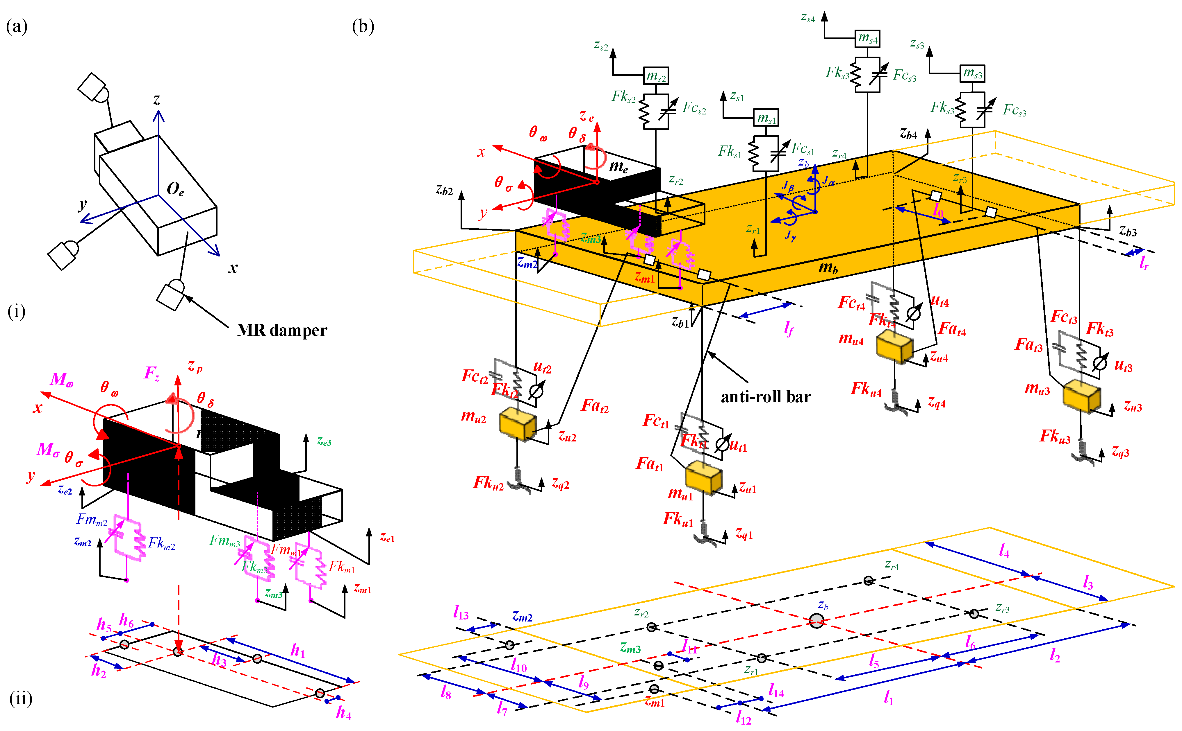
2.1. Active Suspension

When analyzing vehicle ride comfort, the vehicle suspension system is generally simplified into a multi-degree-of-freedom vibration system based on actual conditions. Excitation, springs, damping, and mass are the four major elements of the vibration system [62]. As shown in Figure 1, a 14-degree-of-freedom vehicle dynamics analysis model has been established, considering the nonlinear characteristics of stiffness and damping in the engine mount, suspension, and wheels. This model comprises three degrees of freedom for the engine mount, three degrees of freedom for the vehicle body, one degree of freedom for each unsprung mass (four unsprung masses in total), and one degree of freedom for each seat mass (four seats in total). In addition, the influence of the anti-roll bar is considered [63].

The yawing motion of the engine and vehicle body is ignored. The main reason is that the yawing motion of the engine and vehicle body may not be the main factor affecting overall vibration in certain situations, especially when analyzing other more significant vibration sources such as tire imbalance and pavement unevenness [64]. In addition, existing experimental data or previous studies have shown that under specific operating conditions, the yawing effects of engine suspension and vehicle body can be ignored [65]. But in more detailed or precise research, the yawing effects of engine suspension and vehicle body may need to be reconsidered. As research deepens, the vibration transmission characteristics of engine mounts and the yawing response of the vehicle body at different speeds can be gradually investigated by applying multi-vehicle body dynamics [66,67]. Although we simplified the suspension dynamics model, it can still effectively identify the influence of key parameters, thereby optimizing suspension design to improve the overall performance and ride comfort of the vehicle.

The seats and engine mounts use magnetorheological dampers, while the suspension dampers use hydraulic dampers. The control inputs for the entire vehicle include three parts: the control input for the force actuator of the suspension, the semi-active control input for the magnetorheological damper of the seat, and the semi-active control input for the magnetorheological damper of the engine mount. The external excitation of a vehicle comes from the road surface and the engine. Road excitation is the force and vibration generated during the contact between the vehicle and various road surfaces as it travels. The type and degree of these excitations depend on the unevenness of the road surface [68]. Engine excitation mainly refers to the forces and vibrations produced when the engine is running. These excitations can be transmitted to other parts of the vehicle, affecting the overall performance and ride comfort [69].

(1)

The differential equation for the vertical motion of the unsprung mass in each suspension is shown below:

$$m_{u1}{\ddot{z}}_{u1}=F{c}_{t1}+F{k}_{t1}+F{a}_{t1}-F{k}_{u1}+u_{t1},$$

(1)

$$m_{u2}{\ddot{z}}_{u2}=F{c}_{t2}+F{k}_{t2}+F{a}_{t2}-F{k}_{u2}+u_{t2},$$

(2)

$$m_{u3}{\ddot{z}}_{u3}=F{c}_{t3}+F{k}_{t3}+F{a}_{t3}-F{k}_{u3}+u_{t3},$$

(3)

$$m_{u4}{\ddot{z}}_{u4}=F{c}_{t4}+F{k}_{t4}+F{a}_{t4}-F{k}_{u4}+u_{t4},$$

(4)

where the subscripts 1, 2, 3, and 4, respectively, represent the four vibration points of the vehicle: left-front, right-front, left-rear, and right-rear. m_ui represents the unsprung mass, z_ui represents the displacement of the unsprung mass, Fc_ti represents the damping force on the unsprung mass, Fk_ti represents the spring force on the unsprung mass, Fa_ti represents the force from the anti-roll bar on the unsprung mass, Fk_ui represents the elastic force exerted by the tire, and u_ti is the active force applied by the actuator.

The damping force for the hydraulic damping of the suspension on the unsprung mass Fc_ti (i = 1, 2, 3, and 4) is calculated as follows [70,71,72]:

$$F{c}_{ti}=\left\{\begin{array}{l}{C}_{fb}{v}_{kb}+C_{fb}\left(\left({\dot{z}}_{bi}-{\dot{z}}_{ui}\right)-v_{kb}\right)/{\eta }_{kb}, \left({\dot{z}}_{bi}-{\dot{z}}_{ui}\right)\ge v_{kb},\\ C_{fb}\left({\dot{z}}_{bi}-{\dot{z}}_{ui}\right), 0\le \left({\dot{z}}_{bi}-{\dot{z}}_{ui}\right)<v_{kb},\\ C_{fb}{\beta }_{fb}\left({\dot{z}}_{bi}-{\dot{z}}_{ui}\right), v_{bb}\le \left({\dot{z}}_{bi}-{\dot{z}}_{ui}\right)<0,\\ C_{fb}{\beta }_{fb}{v}_{bb}+C_{fb}{\beta }_{fb}\left(\left({\dot{z}}_{bi}-{\dot{z}}_{ui}\right)-v_{bb}\right)/{\eta }_{bb}, \left({\dot{z}}_{bi}-{\dot{z}}_{ui}\right)<v_{bb},\end{array}\right.,$$

(5)

where C_fb is the equivalent damping, v_kb is the initial opening speed of the damper recovery stroke, η_kb is the ratio of the damping coefficient of the damper opening valve under the recovery stroke to the damping coefficient at maximum opening, β_fb is the two-way damping ratio reflecting the damping resistance of the suspension damper recovery and compression resistance, v_bb is the initial opening speed of the damper compression stroke, η_bb is the ratio of the damping coefficient of damper opening valve under the compression stroke to the damping coefficient at maximum opening. z_bi is the point on the body corresponding to the suspension.

The calculation of the spring force for the helical spring on the unsprung mass, Fk_ti (i = 1, 2, 3, and 4), is as follows [73,74]:

$$F{k}_{ti}=k_{ti}(z_{bi}-z_{ui})+{\epsilon }_t{k}_{ti}{(z_{bi}-z_{ui})}^3,$$

(6)

where k_ti is the equivalent stiffness, and ε_t is the nonlinear coefficient.

The calculation of the anti-roll force Fa_ti acting on the unsprung mass due to the anti-roll bar is as follows [75,76]:

$$F{a}_{t1}=k_{\alpha f}\left(z_{b1}-z_{u1}-(z_{b2}-z_{u2})\right){\displaystyle \frac{(l_3+l_4)}{l_f\cdot {l_0}^2}},$$

(7)

$$F{a}_{t2}=-k_{\alpha f}\left(z_{b1}-z_{u1}-(z_{b2}-z_{u2})\right){\displaystyle \frac{(l_3+l_4)}{l_f\cdot {l_0}^2}},$$

(8)

$$F{a}_{t3}=k_{\alpha r}\left(z_{b3}-z_{u3}-(z_{b4}-z_{u4})\right){\displaystyle \frac{(l_3+l_4)}{l_r\cdot {l_0}^2}},$$

(9)

$$F{a}_{t4}=-k_{\alpha r}\left(z_{b3}-z_{u3}-(z_{b4}-z_{u4})\right){\displaystyle \frac{(l_3+l_4)}{l_r\cdot {l_0}^2}},$$

(10)

where l_f is the vertical distance from the endpoint to the straight rod part of the front suspension, l_r is the vertical distance from the endpoint to the straight rod part of the rear suspension, l₀ is the distance between the two rubber bushes, and l₃ and l₄ represent the distances from the vehicle body to the left and right axles, respectively. k_αf and k_αr are the roll stiffnesses of the front and rear suspensions, respectively.

The elastic force of a tire is the reaction force generated when the tire is subjected to pressure. The elastic force of a tire Fk_ui (i = 1, 2, 3 and 4) is calculated as follows [77]:

$$F{k}_{ui}=k_{ui}(z_{ui}-z_{qi})+{\epsilon }_u{k}_{ui}{(z_{ui}-z_{qi})}^3,$$

(11)

where k_ti is the equivalent stiffness of the tire, ε_u is the nonlinear coefficient of the tire, and z_qi is the excitation displacement of the road surface.

The point on the body corresponding to the suspension z_bi satisfies the following kinematic relationship:

$$z_{b1}=z_b+l_1\beta +l_3\gamma ,$$

(12)

$$z_{b2}=z_b+l_1\beta -l_4\gamma ,$$

(13)

$$z_{b3}=z_b-l_2\beta +l_3\gamma ,$$

(14)

$$z_{b4}=z_b-l_2\beta -l_4\gamma ,$$

(15)

where z_b is the vertical velocity of the center of mass of the vehicle body, β is the pitch angle, γ is the roll angle, and l₁ and l₂ represent the distances from the vehicle body to the front and rear axles.

Table 1. Parameter values for the vertical motion of the unsprung mass.

Parameter	Value	Parameter	Value
mu1	50 kg	ku1	217,751 N/m
mu2	50 kg	ku2	217,751 N/m
mu3	68 kg	ku3	217,751 N/m
mu4	68 kg	ku4	217,751 N/m
l1	1.55 m	lf	0.30 m
l2	1.45 m	lr	0.15 m
l3	0.75 m	l0	0.58 m
l4	0.75 m	kαf	29.4 N·m/°
εu	0.1	kαr	12.8 N·m/°

provides all the parameter values for the vertical motion of the unsprung mass.

Table 2. Parameter values for the hydraulic damping of the suspension.

Parameter	Value	Parameter	Value
Cfb	1290 N·s/m	βfb	0.3
ηkb	1.4	vkb	0.3 m/s
ηbb	1.6	vbb	−0.3 m/s

presents the parameter values for the hydraulic damping of the suspension.

(2)

The vertical motion of the vehicle body is related to the change in contact between the wheels and the ground as the vehicle passes over an uneven road surface. The pitching motion of the vehicle body is most pronounced when the vehicle is accelerating and braking. The control of the pitching motion is critical to improving the dynamic stability and comfort of the vehicle. Roll motion occurs mainly when the vehicle is turning, as the vehicle’s center of gravity shifts to the outside, creating roll. Controlling the roll motion is important to maintain vehicle stability and improve cornering performance. The differential equations for the vertical, pitch, and roll motions of a vehicle are as follows [78,79]:

$$m_b{\ddot{z}}_b=-{\displaystyle \sum _{i=1}^4\left[F{k}_{ti}+F{c}_{ti}+F{a}_{ti}+u_{ti}\right]}+{\displaystyle \sum _{i=1}^4\left[F{k}_{si}+F{c}_{si}\right]}+{\displaystyle \sum _{i=1}^3\left[F{k}_{mi}+F{m}_{mi}\right]},$$

(16)

$$\begin{array}{l}{J}_{\beta }\ddot{\beta }=-{\displaystyle \sum _{i=1,2}{l}_1\left[F{k}_{ti}+F{c}_{ti}+u_{ti}\right]}+{\displaystyle \sum _{i=3,4}{l}_2\left[F{k}_{ti}+F{c}_{ti}+u_{ti}\right]}+{\displaystyle \sum _{i=1,2}{l}_5\left[F{k}_{si}+F{c}_{si}\right]}\\ -{\displaystyle \sum _{i=3,4}{l}_6\left[F{k}_{si}+F{c}_{si}\right]}+(l_1+l_{12})\left[F{k}_{m1}+F{m}_{m1}\right]+(l_1+l_{13})\left[F{k}_{m2}+F{m}_{m2}\right]\\ +(l_1-l_{14})\left[F{k}_{m3}+F{m}_{m3}\right],\end{array}$$

(17)

$$\begin{array}{l}{J}_{\gamma }\ddot{\gamma }=-{\displaystyle \sum _{i=1,3}{l}_3\left[F{k}_{ti}+F{c}_{ti}+u_{ti}\right]}+{\displaystyle \sum _{i=2,4}{l}_4\left[F{k}_{ti}+F{c}_{ti}+u_{ti}\right]}+l_0\left(F{a}_{t1}-F{a}_{t2}\right)/2\\ +l_0\left(F{a}_{t3}-F{a}_{t4}\right)/2+{\displaystyle \sum _{i=1,3}{l}_7\left[F{k}_{si}+F{c}_{si}\right]}-{\displaystyle \sum _{i=2,4}{l}_8\left[F{k}_{si}+F{c}_{si}\right]}\\ +l_9\left[F{k}_{m1}+F{m}_{m1}\right]-l_{10}\left[F{k}_{m2}+F{m}_{m2}\right]+l_{11}\left[F{k}_{m3}+F{m}_{m3}\right],\end{array}$$

(18)

where m_b is the mass of the vehicle body, J_β is the moment of inertia for vehicle body roll, J_γ is the moment of inertia for vehicle body pitch, Fk_si is the spring force of the seat, Fc_si is the magnetorheological damping force of the seat, Fk_mi is the elastic force of the engine mount, Fm_mi is the magnetorheological damping force of the engine mount, l₅ and l₆ are the distances from the front and rear seats to the body center-of-mass axes, l₇ and l₈ are the distances from the left and right seats to the body center-of-mass axes, l₉, l₁₀, and l₁₁ are the distances from engine mounts 1, 2, and 3 to the body center of mass axis, and l₁₂, l₁₃, and l₁₄ are the distances from engine mounts 1, 2, and 3 to the front axle, respectively.

The calculation of the spring force of the seat Fk_si (i = 1, 2, 3 and 4) is as follows [80]:

$$F{k}_{si}=k_{si}(z_{si}-z_{ri})+{\epsilon }_s{k}_{si}{(z_{si}-z_{ri})}^3,$$

(19)

where k_si is the equivalent stiffness of the seat, ε_s is the nonlinear coefficient of the seat, z_si is the vertical displacement of the seat, and z_ri is the action point on the suspension corresponding to the seat. In seat design, magnetorheological damping technology can be used to improve ride comfort and safety. The calculation of the magnetorheological damping force Fc_si (i = 1, 2, 3 and 4) in seats is as follows [81]:

$$\begin{array}{l}F{c}_{si}=f_0+(k_{d,2}{\widehat{\phi }}_{si}^2+k_{d,1}{\widehat{\phi }}_{si}+k_{d,0})(z_{si}-z_{ri})+(c_{po,2}{\widehat{\phi }}_{si}^2+c_{po,1}{\widehat{\phi }}_{si}+c_{p,0})({\dot{z}}_{si}-{\dot{z}}_{ri})\\ +\left(m_{f,2}{\widehat{\phi }}_{si}^2+m_{f,1}{\widehat{\phi }}_{si}+m_{f,0}\right)({\ddot{z}}_{si}-{\ddot{z}}_{ri})\\ +\left(f_{y,2}{\widehat{\phi }}_{si}^2+f_{y,1}{\widehat{\phi }}_{si}+f_{y,0}\right)\tan \mathrm{sig}\left((({\dot{z}}_{si}-{\dot{z}}_{ri})+{\lambda }_1\mathrm{sgn}({\ddot{z}}_{si}-{\ddot{z}}_{ri}))({\lambda }_{2,2}{\widehat{\phi }}_{si}^2+{\lambda }_{2,1}{\widehat{\phi }}_{si}+{\lambda }_{2,0})\right).\end{array}$$

(20)

where ${\widehat{\phi }}_{si}$ is the magnetorheological voltage inputting into the damping force of the seat, and all parameters can be referred to in the literature [81]. Excessive magnetorheological voltage may lead to overheating of the magnetorheological material or the surrounding equipment, and a higher voltage also means more energy consumption. If the magnetorheological voltage is too low, it may not sufficiently activate the magnetorheological material, resulting in performance that does not meet expectations, such as insufficient damping or control strength. Therefore, to ensure the performance and safety of the magnetorheological damper, the magnetorheological voltage needs to meet the following constraints [81,82]:

$${\widehat{\phi }}_{si}=\left\{\begin{array}{l}{\phi }_{smax}=2.5, {\widehat{\phi }}_{si}>{\phi }_{smax}\\ {\widehat{\phi }}_{si}, {\phi }_{smax}>{\widehat{\phi }}_{si}>{\phi }_{smin}\\ {\phi }_{smin}=0,{\widehat{\phi }}_{si}<{\phi }_{smin}\end{array}\right..$$

(21)

On the basis of sky-hook control, the expected damping force is as follows [83]:

$$F{k}_{si}=\left\{\begin{array}{l}{\left.F{k}_{si}\right|}_{{\stackrel{⌢}{\phi }}_{si}\ne 0}, ({\dot{z}}_{si}-{\dot{z}}_{ri}){\dot{z}}_{si}\ge 0,\\ {\left.F{k}_{si}\right|}_{{\stackrel{⌢}{\phi }}_{si}=0}, ({\dot{z}}_{si}-{\dot{z}}_{ri}){\dot{z}}_{si}<0,\end{array}\right. .$$

(22)

If the direction of body displacement velocity is opposite to the direction of damper compression velocity, no damper is used; if the direction of body displacement velocity is the same as the direction of damper compression velocity, a damper is used. This provides a good balance between body vibration and unsprung mass vibration. The action point on the suspension corresponding to the seat z_ri satisfies the following kinematic relationship:

$$z_{r1}=z_b+l_5\beta +l_7\gamma ,$$

(23)

$$z_{r2}=z_b+l_5\beta -l_8\gamma ,$$

(24)

$$z_{r3}=z_b-l_6\beta +l_7\gamma ,$$

(25)

$$z_{r4}=z_b-l_6\beta -l_8\gamma ,$$

(26)

The calculation of the spring force of the engine mount Fk_mi (i = 1, 2, and 3) is as follows [84]:

$$F{k}_{mi}=k_{mi}(z_{ei}-z_{mi})+{\epsilon }_m{k}_{mi}{(z_{ei}-z_{mi})}^3,$$

(27)

where k_mi is the equivalent stiffness of the seat, ε_m is the nonlinear coefficient of the seat, z_ei is the action point on the engine mount corresponding to the engine, and z_mi is the action point on the vehicle body corresponding to the engine mount. The use of magnetorheological dampers in engine mounts can effectively reduce vibration and noise caused by engine operation. The magnetorheological damping force Fm_mi (i = 1, 2, and 3) for the engine mount is calculated as follows [81]:

$$\begin{array}{l}F{m}_{mi}=f_0+(k_{d,2}{\widehat{\phi }}_{ei}^2+k_{d,1}{\widehat{\phi }}_{ei}+k_{d,0})(z_{ei}-z_{mi})+(c_{po,2}{\widehat{\phi }}_{ei}^2+c_{po,1}{\widehat{\phi }}_{ei}+c_{p,0})({\dot{z}}_{ei}-{\dot{z}}_{mi})\\ +\left(m_{f,2}{\widehat{\phi }}_{ei}^2+m_{f,1}{\widehat{\phi }}_{ei}+m_{f,0}\right)({\ddot{z}}_{ei}-{\ddot{z}}_{mi})\\ +\left(f_{y,2}{\widehat{\phi }}_{ei}^2+f_{y,1}{\widehat{\phi }}_{ei}+f_{y,0}\right)\tan \mathrm{sig}\left((({\dot{z}}_{ei}-{\dot{z}}_{mi})+{\lambda }_1\mathrm{sgn}({\ddot{z}}_{ei}-{\ddot{z}}_{mi}))({\lambda }_{2,2}{\widehat{\phi }}_{ei}^2+{\lambda }_{2,1}{\widehat{\phi }}_{ei}+{\lambda }_{2,0})\right).\end{array}$$

(28)

where ${\widehat{\phi }}_{ei}$ is the magnetorheological voltage inputting into the damping force of the engine mount, and all parameters mentioned are referenced in the literature [81]. Research indicates that an appropriate range of voltage can help magnetorheological systems maintain high performance while optimizing energy efficiency. The magnetorheological voltage ${\widehat{\phi }}_{ei}$ meets the following constraints [81,85]:

$${\widehat{\phi }}_{ei}=\left\{\begin{array}{l}{\phi }_{emax}=1.5, {\widehat{\phi }}_{ei}>{\phi }_{emax}\\ {\widehat{\phi }}_{ei}, {\phi }_{emax}>{\widehat{\phi }}_{ei}>{\phi }_{emin}\\ {\phi }_{emin}=0,{\widehat{\phi }}_{ei}<{\phi }_{emin}\end{array}\right..$$

(29)

The expected damping force for engine vibration damping is as follows [86]:

$$F{m}_{mi}=\left\{\begin{array}{l}{\left.F{m}_{mi}\right|}_{{\stackrel{⌢}{\phi }}_{ei}\ne 0}, ({\dot{z}}_{mi}-{\dot{z}}_{ei}){\dot{z}}_{mi}\ge 0,\\ {\left.F{m}_{mi}\right|}_{{\stackrel{⌢}{\phi }}_{ei}=0}, ({\dot{z}}_{mi}-{\dot{z}}_{ei}){\dot{z}}_{mi}<0,\end{array}\right..$$

(30)

The action point on the engine mount corresponding to the engine z_ei satisfies the following kinematic relationship:

$$z_{e1}=z_p+h_1\sigma +h_4\omega ,$$

(31)

$$z_{e2}=z_p-h_2\sigma -h_5\omega ,$$

(32)

$$z_{e3}=z_p+h_3\sigma +h_6\omega ,$$

(33)

where z_p is the vertical displacement of the center of mass of the engine, σ is the engine roll angle, and ω is the engine pitch angle. The action point on the vehicle body corresponding to the engine mount z_mi satisfies the following kinematic relationship:

$$z_{m1}=z_b+\left(l_1+l_{12}\right)\beta +l_9\gamma ,$$

(34)

$$z_{m2}=z_b+(l_1+l_{13})\beta -l_{10}\gamma ,$$

(35)

$$z_{m3}=z_b+\left(l_1-l_{14}\right)\beta +l_{11}\gamma ,$$

(36)

Table 3. Parameter values for the vertical motion of the vehicle body.

Parameter	Value	Parameter	Value
mb	1350 kg	l11	0.05 m
Jβ	5368 kg∙m2	l12	0.15 m
Jγ	529 kg∙m2	l13	0.27 m
l5	0.15 m	l14	0.10 m
l6	0.53 m	kt1	24,606 N/m
l7	0.35 m	kt2	24,606 N/m
l8	0.35 m	kt3	26,115 N/m
l9	0.50 m	kt4	26,115 N/m
l10	0.50 m	εt	0.12
ks1	22,000 N/m	ks2	22,000 N/m
ks3	17,000 N/m	ks4	17,000 N/m
εs	0.11	km3	250,000 N/m
km1	250,000 N/m	εm	0.1
km2	250,000 N/m

lists the parameter values for the vertical motion of the vehicle body, and

Table 4. Parameter values for the magnetorheological damper [81].

Parameter	Value	Parameter	Value
kd,2	−68.2 N/m	fy,2	−51.7 N
kd,1	−1156.5 N/m	fy,2	439.7 N
kd,0	10,236.7 N/m	fy,2	134.8 N
cpo,2	162.1 N·s/m	λ2,2	−11.6907 s/m
cpo,1	711.0 N·s/m	λ2,1	11.1987 s/m
cpo,0	871.9 N·s/m	λ2,0	137.7681 s/m
mf,2	−0.207,1 kg	f0	80.0 N
mf,1	0.4785 kg	λ1	0.000016 s/m
mf,0	0.6638 kg

lists the parameter values for the magnetorheological damper.

(3)

Seat vibration involves considering the mass of the seat, spring stiffness, and damping coefficient. It can be modeled by a second-order linear differential equation, as follows [87,88]:

$$m_{si}{\ddot{z}}_{si}=-F{k}_{si}-F{c}_{si},$$

(37)

where m_si (i = 1, 2, 3, and 4) is the total mass of the seat and the human body, and z_si is the vertical displacement of the seat.

Table 5. Parameter values for the seat vibration.

Parameter	Value	Parameter	Value
ms1	80 kg	ms2	80 kg
ms3	85 kg	ms4	85 kg

lists the parameter values for the seat vibration.

(4)

The vertical, rolling, and pitching movements of the engine are related to the motion of the pistons. The rapid up-and-down movement of the pistons in the cylinders generates vibrations, which are transmitted to the vehicle body through the engine mounts, potentially causing vertical movement, rolling, and pitching of the engine. The differential equations for the vertical, rolling, and pitching movements of the engine are as follows [89,90]:

$$m_e{\ddot{z}}_p=-{\displaystyle \sum _{i=1}^3\left(F{k}_{mi}+F{m}_{mi}\right)}+F_z,$$

(38)

$${\theta }_{\sigma }\ddot{\sigma }=-\left(F{k}_{m1}+F{m}_{m1}\right)h_1+\left(F{k}_{m2}+F{m}_{m2}\right)h_2-\left(F{k}_{m3}+F{m}_{m3}\right)h_3+M_{\sigma },$$

(39)

$${\theta }_{\omega }\ddot{\omega }=-\left(F{k}_{m1}+F{m}_{m1}\right)h_4+\left(F{k}_{m2}+F{m}_{m2}\right)h_5-\left(F{k}_{m3}+F{m}_{m3}\right)h_6+M_{\omega },$$

(40)

where m_e is the mass of the engine, θ_σ is the roll moment of inertia of the engine, θ_ω is the pitch moment of inertia of the engine, F_z is the vertical component of centrifugal inertia force in the reciprocating motion of the engine, M_σ is the additional torque in the y-direction during the reciprocating motion of the engine, M_ω is the additional torque in the x-direction during the reciprocating motion of the engine, h₁, h₂, and h₃ are the distances from engine mounts 1, 2, and 3 to the longitudinal axis of the engine, and h₄, h₅, and h₆ are the distances from engine mounts 1, 2, and 3 to the horizontal axis of engine, respectively. In addition to road excitation, there is also internal excitation, namely engine vibration. The engine studied in this article is a four-in-line engine, and the main reasons for its vibration are the cyclic gas pressure in the cylinder, the reciprocating inertia force, and the centrifugal inertia force generated by the crank-connecting rod-piston mechanism movement. According to the literature [91], F_z, M_σ, and M_ω are calculated as follows:

$$F_z=4m_{c}r\lambda {\varpi }^2\cos (2\varpi t),$$

(41)

$$M_{\sigma }=4m_{c}r\lambda {\varpi }^2\cos (2\varpi t)L,$$

(42)

$$M_{\omega }=M_e[1+1.3\sin (2\varpi t)],$$

(43)

where m_c is the reciprocating mass of a piston, r is the radius of a crank, λ is the ratio of r to the length of the shaft, ϖ = 2πn/60 is the rotational frequency of the crank, t is the time, L is the distance between the center-of-gravity, and the center-line of the second and third cylinders M_e = −6.8′10⁻⁶n² + 0.059n + 112.5 is the mean value of the torque of the engine with maximum fuel consumption. Here, n (r/min) is the rotation speed of the engine. Typically, as the engine’s rotational speed increases, its vibrations also increase. This is due to the fact that at higher speeds, the forces exerted on internal components such as pistons, crankshafts, and connecting rods are greater, leading to faster movements and resulting in more significant dynamic imbalances [92,93].

There is a correlation between the speed of rotation of the engine n and the speed of the vehicle u, but this relationship is not a simple one-to-one correspondence. This is due to the presence and role of the gearbox, which regulates the ratio between engine speed and wheel speed through different gears.

$$n={\displaystyle \frac{u{i}_{\mathrm{g}}{i}_0}{0.377r_{wheel}}}$$

(44)

where i_g is the transmission ratio of the gear reducer (i_g1 = 3.6, i_g2 = 2.125, i_g3 = 1.458, i_g4 = 1.071, i_g5 = 0.857), i₀ (=4.313) is the transmission ratio of the main reducer, and r_wheel (=0.326 m) is the radius of the wheel. The gear shifting strategy of the transmission is controlled by the speed of the vehicle. Speeds below 15 km/h correspond to first gear, speeds from 15 to 25 km/h shift to second gear, speeds from 25 to 45 km/h shift to third gear, speeds from 45 to 60 km/h shift to fourth gear, and speeds above 60 km/h shift to fifth gear.

Table 6. Parameter values for the engine.

Parameter	Value	Parameter	Value
me	230 kg	θσ	6.54 kg∙m2
θω	11.84 kg∙m2	h1	0.48 m
h2	0.45 m	h3	0.15 m
h4	0.06 m	h5	0.04 m
h6	0.35 m

presents the parameter values for the engine, while

Table 7. Parameter values for the crank-connecting rod-piston mechanism.

Parameter	Value	Parameter	Value
mc	0.82 kg	L	0.015 m
λ	0.33	r	0.06 m

lists the parameter values for the crank-connecting rod-piston mechanism.

2.2. Road Excitation

2.2.1. Single-Wheel Road Input Analysis

The variation q(I) of the height q of the pavement relative to the reference plane, along the length I of the roadway alignment, is called the pavement unevenness function. It is a stochastic function and its statistical properties can only be analyzed from random signal theory [94]. According to the stochastic vibration theory, the pavement unevenness in the case of a vehicle traveling at a uniform speed can be regarded as a stationary stochastic process with ergodicity. Therefore, the frequency-domain model and time-domain model of random road excitation can be established.

As an external input to the vehicle suspension system, the random road excitation is commonly characterized by the power spectrum density (PSD) of the road surface. The spectral power density at the spatial frequency domain can be mathematically expressed as follows: [95]:

$$G_q\left(n\right)=\underset{\mathsf{\Delta }n\to 0}{\lim }{\displaystyle \frac{{\sigma }_{q~\mathsf{\Delta }n}^2}{\mathsf{\Delta }n}},$$

(45)

where ${\sigma }_{q~\mathsf{\Delta }n}^2$ is the “power” corresponding to the frequency band ∆n, n is the number of waves per unit length (i.e., the spatial frequency). In 1984, the International Organization for Standardization proposed a draft method for representing road roughness in the document ISO/TC 108/SC2N67, which includes a fitting expression for the power spectrum density of pavement unevenness, G_q(n), expressed by the following [96]:

$$G_q(n)=G_q(n_0){({\displaystyle \frac{n}{n_0}})}^{-w} (n_{min}\le n\le n_{max}),$$

(46)

where n (m⁻¹) represents the spatial frequency, indicating the number of wavelengths per meter. n₀ = 0.1 m⁻¹ is the reference spatial frequency, G_q(n₀) (m³) is the road roughness coefficient, representing the road displacement power spectral density at the reference spatial frequency. w is the frequency exponent, which determines the frequency structure of the road displacement power spectral density and is typically taken as w = 2. n_min and n_max, respectively, represent the lower and upper limits of the spatial frequency, typically set at n_min = 0.011 m⁻¹ and n_max = 2.83 m⁻¹ (0.011 m⁻¹ < n < 2.83 m⁻¹). According to the different road displacement power spectral densities, road roughness is divided into eight grades from A to H.

Table 8. Pavement roughness categorization across eight distinct levels [96].

Category	Gq(n0)/(10−6 m3) (n0 = 0.1 m−1)	σq/(10−3 m)
A	16	3.81
B	64	7.61
C	256	15.23
D	1024	30.45
E	4096	60.90
F	16384	121.89
G	65536	243.61
H	262144	487.22

provides the geometric mean values of the road roughness coefficients under different road grades at n₀ = 0.1 m⁻¹ and w = 2, and it also lists the geometric mean values.

The power spectral density mentioned above is a spatial power spectrum. In practical analysis, it is necessary to introduce the variable of vehicle speed to convert the spatial power spectrum into a time power spectrum. When a vehicle travels at a constant speed u over a road surface with spatial frequency n, the following formula can be derived:

$$f=un,$$

(47)

where f (s⁻¹) represents the time frequency. From this, the conversion formula between spatial frequency power spectral density and temporal frequency power spectral density can be derived:

$$G_q\left(f\right)=\underset{\mathsf{\Delta }n\to 0}{\lim }{\displaystyle \frac{{\sigma }_{q~\mathsf{\Delta }n}^2}{u\mathsf{\Delta }n}}={\displaystyle \frac{G_q\left(n\right)}{u}}=G_q\left(n_0\right)n_0^2{\displaystyle \frac{u}{f^2}}.$$

(48)

Considering the spatial lower cutoff frequency n_min and the temporal lower cutoff frequency f_min = un_min, the following equation holds [97]:

$$G_q(f)=G_q(n_0)n_0^2{\displaystyle \frac{u}{f^2+f_{min}^2}}.$$

(49)

Common methods for generating time-domain models of road surfaces include the filtered white noise method [98], harmonic superposition method [99], auto-regressive model (AR) [100], and auto-regressive moving average (ARMA) method [101]. Random road roughness can be regarded as a type of noise with limited bandwidth, which can be obtained through the transformation of ideal, infinite bandwidth, and constant PSD white noise through certain rules. A time-domain random road excitation model can be established based on the filtered white noise method. The filtering white noise method is based on the assumption that the road excitation q(t) is treated as the response of a first-order linear system with unit white noise w(t) input. In a first-order filter white noise system, which is a single degree of freedom linear system, the relationship between the response quantity and the excitation quantity in terms of power spectral density is as follows:

$$G_q(f)={\left|H_{q-w}(f)\right|}^2{G}_w(f),$$

(50)

where H_q−w(f) is the frequency response function between the excitation quantity and the response quantity, G_w(f) is the power spectral density of the excitation quantity, and G_q(f) is the power spectral density of the response quantity. The time-domain representation of a first-order filter white noise system is as follows:

$$\dot{q}(t)+aq(t)=bw(t),$$

(51)

where a and b are parameters of the system architecture. Performing a Fourier transform on the above equation yields:

$$q(f)\cdot (2\pi f\cdot j+a)=b\cdot w(f).$$

(52)

The frequency response function between the excitation quantity and the response quantity, H_q−w(f), can be obtained:

$${\left|H_{q-w}(f)\right|}^2={\displaystyle \frac{b^2}{a^2+{(2\pi f)}^2}}.$$

(53)

The structural parameters of a first-order filter white noise system are as follows:

$$\left\{\begin{array}{l}a=2\pi f_{min}\\ b=2\pi n_0\sqrt{G_q(n_0)u}\end{array}\right..$$

(54)

The road excitation model can be established through the filtered white noise approach, as demonstrated in the following formulation [102]:

$$\dot{q}(t)+2\pi f_{min}q(t)=2\pi n_0\sqrt{G_q(n_0)u}w(t).$$

(55)

The current problem is how to generate the stochastic road spectra of the other three wheels using the road excitation of the left front wheel.

2.2.2. Temporal Displacement of Axle Trajectories During Vehicle Motion

We use the subscripts f and r to denote the front axle and the rear axle, respectively. The front and rear wheels pass over the same surface, with the rear wheel experiencing a time delay τ relative to the front wheel, where τ is (l₁ + l₂)/u. The relationship between the front and rear road excitations is as follows [103]:

$$q_r(t)=q_f(t-\tau ).$$

(56)

The Fourier transform of the above equation can be obtained as follows:

$$q_r(\omega )=q_f(\omega )e^{-j\omega \tau },$$

(57)

where q_r(ω) is the Fourier transform of q_r(t), and q_f(ω) is the Fourier transform of q_f(t). By using the first-order Pade approximation to equivalently calculate the time delay system, the transfer function G_r−f(ω) of the road excitation from the rear wheel to the front wheel is as follows:

$$G_{r-f}(\omega )=q_r(\omega )/q_f(\omega )=e^{-j\omega \tau }=\left(1-j\omega \tau /2\right)/\left(1+j\omega \tau /2\right).$$

(58)

By performing the inverse Laplace transform, we obtain:

$${\dot{q}}_r(t)=-2q_r(t)/\tau +2q_f(t)/\tau -{\dot{q}}_f(t).$$

(59)

2.2.3. Coherence of Left and Right Wheel Tracks

We use the subscripts l and r to denote the front axle and the rear axle, respectively. The statistical characteristics of road roughness for two different wheel trajectories on the same road are the same, that is, the auto-correlation power spectral density of the road excitation at the left-side wheel and the road excitation at the right-side wheel are the same. Therefore, the following equation holds:

$$G_{ll}\left(\omega \right)=G_{rr}\left(\omega \right)=G_q\left(\omega \right),$$

(60)

where G_ll(ω) and G_rr(ω) are the auto-correlation power spectral densities of the road excitation at the left and right wheels, respectively. There is coherence between the left wheel road excitation q_l(t) and the right wheel road excitation q_r(t).

To consider the correlation of the left and right wheels, it is assumed that the white noise w_r(t) used to generate the road spectrum of the right-side wheel can be regarded as the response of a double-input linear system with the inputs of the white noise w_l(t) used to generate the road spectrum of left-side wheel and another white noise w_z(t) that is unrelated to w_l(t). The frequency response function corresponding to w_l(t) is H_r−l(ω), and the following equation holds [104]:

$$w_r\left(\omega \right)=H_{r-l}\left(\omega \right)w_l\left(\omega \right)+H_{r-\mathrm{z}}\left(\omega \right)w_z\left(\omega \right).$$

(61)

Assuming that the time-domain road excitation of left-side wheel q_l(t) is the input of the system, the time-domain road excitation of right-side wheel q_r(t) is the output of the system, and the cross-correlation power spectral density between the time-domain road excitation of the left-side wheel and the time-domain road excitation of the right-side wheel is G_lr(ω), the relationship between the cross-correlation power spectral density between the system input and system output and the auto-correlation power spectral density of system input is as follows:

$$G_{lr}\left(\omega \right)=H_{r-l}\left(\omega \right)G_{ll}\left(\omega \right),$$

(62)

The coherence function between the time-domain road excitation of the left wheel and the time-domain road excitation of the right wheel can be defined as follows:

$${\mathrm{coh}}_{lr}^2\left(\omega \right)={\displaystyle \frac{{‖G_{lr}\left(\omega \right)‖}^2}{G_{ll}\left(\omega \right)G_{rr}\left(\omega \right)}}={\displaystyle \frac{{‖G_{lr}\left(\omega \right)‖}^2}{G_q\left(\omega \right)G_q\left(\omega \right)}}.$$

(63)

Therefore, the following equation holds:

$$H_{r-l}\left(\omega \right)={\mathrm{coh}}_{lr}\left(\omega \right),$$

(64)

The relationship between the auto-power spectral density of white noise w_r(t) and the self-power spectral density of w_l(t) and w_z(t) is as follows:

$$G_{wr}\left(\omega \right)={‖H_{r-l}\left(\omega \right)‖}^2{G}_{wl}\left(\omega \right)+{‖H_{r-\mathrm{z}}\left(\omega \right)‖}^2{G}_{wz}\left(\omega \right),$$

(65)

where G_wr(ω) is the auto-power spectral density of white noise w_r(t), G_wl(ω) is the auto-power spectral density of white noise w_l(t), and G_wz(ω) is the auto-power spectral density of white noise w_z(t). Since w_r(t), w_l(t), and w_z(t) are all unit white noise, their power spectral density is always 1, so the following equation holds:

$$1={‖H_{r-l}\left(\omega \right)‖}^2+{‖H_{r-\mathrm{z}}\left(\omega \right)‖}^2.$$

(66)

A universal formula for the coherence function is as follows [105]:

$${\mathrm{coh}}_{lr}^2\left(\omega \right)=e^{-{\displaystyle \frac{\rho \left(l_3+l_4\right)}{\pi u}}\omega },$$

(67)

where ρ is the adjustment parameter, ρ = 3.4. Applying second-order Pade approximation to equivalent the above equation, the following relationships clearly hold:

$$H_{r-l}\left(j\omega \right)={\displaystyle \frac{a_0+a_{1}j\omega +a_2{\left(j\omega \right)}^2}{b_0+b_{1}j\omega +b_2{\left(j\omega \right)}^2}},$$

(68)

$$H_{r-z}\left(j\omega \right)={\displaystyle \frac{c_0+c_{1}j\omega +c_2{\left(j\omega \right)}^2}{b_0+b_{1}j\omega +b_2{\left(j\omega \right)}^2}}.$$

(69)

The coefficients are defined as follows [106]: a₀ = 1.000, a₁ = 0.0736k, and a₂ = 0.0239k², where k is the ratio ρ(l₃ + l₄)/πu. Additionally, the b-series coefficients are b₀ = 1.0696, b₁ = 2.8390k, and b₂ = 0.8330k², while the c-series parameters are expressed as c₀ = 0.3795, c₁ = 2.6367k, and c₂ = 0.8327k². By defining the intermediate state variable ξ(t) = [ξ₁(t), ξ₂(t)]^T and ψ(t) = [ψ₁(t), ψ₂(t)]^T, we can break down the given equation into two separate state equations:

$$\left(\begin{array}{c}{\dot{\xi }}_1(t)\\ {\dot{\xi }}_2(t)\end{array}\right)=\left(\begin{array}{cc}-{\displaystyle \frac{b_1}{b_2}}& -{\displaystyle \frac{b_0}{b_2}}\\ 1& 0\end{array}\right)\left(\begin{array}{c}{\xi }_1(t)\\ {\xi }_2(t)\end{array}\right)+\left(\begin{array}{c}{\displaystyle \frac{1}{b_2}}\\ 0\end{array}\right)w_l\left(t\right),$$

(70)

$$\left(\begin{array}{c}{\dot{\psi }}_1(t)\\ {\dot{\psi }}_2(t)\end{array}\right)=\left(\begin{array}{cc}-{\displaystyle \frac{b_1}{b_2}}& -{\displaystyle \frac{b_0}{b_2}}\\ 1& 0\end{array}\right)\left(\begin{array}{c}{\psi }_1(t)\\ {\psi }_2(t)\end{array}\right)+\left(\begin{array}{c}{\displaystyle \frac{1}{b_2}}\\ 0\end{array}\right)w_z\left(t\right),$$

(71)

The temporal representation of the stochastic process associated with the right wheel path’s broadband noise signal can be mathematically formulated as follows:

$$\begin{array}{l}{w}_r\left(t\right)=\left(\begin{array}{cc}{a}_1-{\displaystyle \frac{a_2{b}_1}{b_2}}& a_0-{\displaystyle \frac{a_2{b}_0}{b_2}}\end{array}\right)\left(\begin{array}{c}{\xi }_1(t)\\ {\xi }_2(t)\end{array}\right)+{\displaystyle \frac{a_2}{b_2}}{w}_l\left(t\right)\\ +\left(\begin{array}{cc}{c}_1-{\displaystyle \frac{c_2{b}_1}{b_2}}& c_0-{\displaystyle \frac{c_2{b}_0}{b_2}}\end{array}\right)\left(\begin{array}{c}{\psi }_1(t)\\ {\psi }_2(t)\end{array}\right)+{\displaystyle \frac{c_2}{b_2}}{w}_z\left(t\right).\end{array}$$

(72)

Consequently, the time-dependent model describing the road surface excitation acting on the right-wheel is comprehensively formulated as follows:

$${\dot{q}}_r(t)+2\pi f_{min}q(t)=2\pi n_0\sqrt{G_q\left(n_0\right)u}\cdot w_r(t).$$

(73)

2.2.4. Four-Wheels Road Excitation Model

The road excitations for the front left wheel, front right wheel, rear left wheel, and rear right wheel of a car are represented as q₁(t), q₂(t), q₃(t), and q₄(t), respectively. Their expressions are as follows:

$${\dot{q}}_1(t)+2\pi f_{min}{q}_1(t)=2\pi n_0\sqrt{G_q(n_0)u}{w}_l(t),$$

(74)

$${\dot{q}}_2(t)+2\pi f_{min}{q}_2(t)=2\pi n_0\sqrt{G_q(n_0)u}{w}_l(t),$$

(75)

$${\dot{q}}_3(t)=-2q_3(t)/\tau +2q_1(t)/\tau -{\dot{q}}_1(t).$$

(76)

$${\dot{q}}_4(t)=-2q_4(t)/\tau +2q_2(t)/\tau -{\dot{q}}_2(t).$$

(77)

Figure 2 illustrates the road excitations encountered during a simulated journey. Figure 2a presents the speed–time curve, where the vehicle accelerates from 0 km/h to 100 km/h within 20 s, maintains a constant speed for 60 s, and then decelerates back to 0 km/h over another 20 s. Figure 2b shows the road height profile on the C-level road, with variations ranging between −0.1 m and 0.1 m, representing the unevenness of the road surface. Lastly, Figure 2c depicts the road surface spectrum derived from the road height profile, providing a frequency-domain representation of the surface irregularities. Figure 2 collectively characterizes the dynamic road conditions, contributing to the analysis of vehicle performance and ride comfort under varying speed and road surface profiles.

3. Methods

3.1. Fractional-Order PI^λD^μ

3.1.1. Theoretical Framework of Fractional-Order Calculus

In recent years, fractional-order derivatives have become an important tool for describing various complex mechanical and physical behaviors, and thus the study of numerical algorithms for fractional-order differential equations has also received considerable attention. Several definitions exist for fractional-order derivatives, including the Riemann–Liouville, Caputo, and Grünwald–Letnikov fractional-order derivatives [107].

The Grünwald–Letnikov method approximates the derivatives of a function using finite differences. Since the Grünwald–Letnikov formula involves the summation of an infinite series, in practical computations, it is necessary to truncate this series, and the truncation error can affect the results of numerical calculations. If the function f(t) has continuous derivatives up to order m + 1 on the interval [t₀, t], and when α > 0, m must be at least [α]. Then, the Grünwald–Letnikov fractional-order derivative for the order α (m ≤ α < m + 1) of function f(t) is defined as follows [108]:

$${}_{t0}{}^{GL}D_t^{\alpha }f\left(t\right)=\underset{h\to 0}{\lim }\frac{1}{h^{\alpha }}{\displaystyle \sum }_{j=0}^{\left[\left(t-t_0\right)/h\right]}{(-1)}^j\left(\begin{array}{l}\alpha \hfill \\ j\hfill \end{array}\right)f\left(t-jh\right),t>0,\alpha \in R^{+},$$

(78)

where [·] is the Round operator, α is the order, t₀ and t are the lower limit and the upper limit, and

$$\left(\begin{array}{l}\alpha \hfill \\ j\hfill \end{array}\right)={\displaystyle \frac{\alpha \left(\alpha +1\right)\cdots \left(\alpha +j-1\right)}{j!}}={\displaystyle \frac{\alpha !}{j!\left(\alpha -j\right)!}}.$$

(79)

This definition applies equally to differentiation for α > 0 and integration for α < 0. Additionally, if α = 0, according to the definition of the Grünwald–Letnikov fractional derivative, we obtain ${}_{t_0}{}^{GL}D_t^{0}f\left(t\right)=f\left(t\right)$.

The Riemann–Liouville fractional-order derivative was the first to be proposed, and its theoretical analysis is relatively well developed. Riemann–Liouville formulation for fractional-order integration is defined as follows [109]:

$${}_{t_0}{}^{RL}D_t^{-\alpha }f(t)={\displaystyle \frac{1}{\Gamma (\alpha )}}{\displaystyle {\int }_{t_0}^t\frac{f(\tau )}{{(t-\tau )}^{1-\alpha }}}d\tau ,$$

(80)

where Γ(n − α) is the Gamma function. If α > 0 is any positive real number and n is the smallest positive integer greater than α, i.e., n − 1 ≤ α < n, then the Riemann–Liouville fractional-order derivative is defined as follows:

$${}_{t_0}{}^{RL}D_t^{\alpha }f\left(t\right)={\displaystyle \frac{1}{\Gamma \left(n-\alpha \right)}}{\displaystyle \frac{d^n}{d{t}^n}}{{\displaystyle \int }}_{t_0}^t{\displaystyle \frac{f\left(\tau \right)}{{(t-\tau )}^{\alpha -n+1}}}d\tau ,$$

(81)

where n = [α]. The Grünwald–Letnikov and Riemann–Liouville fractional calculus are more suitable for dynamical systems with initial conditions set to zero. The initial conditions of a fractional-order system cannot be completely determined by a fixed value at the initial moment alone, but are closely related to all the states of the system during the pre-initial process, which in fact reflects the long-memory property of fractional-order systems.

In the study of systems with non-zero initial conditions, Caputo fractional calculus is applicable. The definition of the Caputo fractional-order derivative is essentially the same as that of the Riemann–Liouville fractional-order derivative, except that the order of differentiation and integration is reversed. The Riemann–Liouville fractional-order derivative integrates first and then differentiates, whereas the Caputo fractional-order derivative differentiates first and then integrates. The α-th order Caputo derivative of a function f(t) is defined as follows [110]:

$${}_{t_0}{}^{C}D_t^{\alpha }f\left(t\right)={\displaystyle \frac{1}{\Gamma \left(m-\alpha \right)}}{{\displaystyle \int }}_{t_0}^t{\displaystyle \frac{f^{\left(m\right)}\left(\tau \right)}{{(t-\tau )}^{1+\alpha -m}}}d\tau ,$$

(82)

where m = [α]. The Caputo formulation defines fractional-order integration as follows:

$${}_{t_0}{}^{C}D_t^{-\alpha }f\left(t\right)={\displaystyle \frac{1}{\Gamma \left(\gamma \right)}}{{\displaystyle \int }}_{t_0}^t{\displaystyle \frac{f\left(\tau \right)}{{(t-\tau )}^{1-\alpha }}}d\tau .$$

(83)

Grünwald–Letnikov fractional calculus is defined on a series of numerical points and is therefore widely used in various numerical calculations. When the value of h is small enough, Grünwald–Letnikov fractional calculus can have high computational accuracy [111]. The values of the FOPID model in the time domain are computed based on the Grünwald–Letnikov fractional-order calculus.

3.1.2. Architecture of PI^λD^μ Controller System

In the context of active suspension systems, a sophisticated mathematical model is employed to characterize the behavior and performance of the suspension mechanism. The state vector, denoted as X, encapsulates the system’s internal state variables, reflecting significant parameters such as displacement and velocity of both the sprung and unsprung masses. The output variable, represented by Y, typically includes parameters of interest such as ride comfort, handling performance, and road stability, which are directly influenced by the system’s dynamics. The controller input, labeled as U, signifies the control actions or adjustments made by the suspension system in response to variations in external conditions, thereby facilitating real-time adaptation to changing road profiles and driving scenarios. Lastly, the external excitation, denoted as Z, signifies the disturbances acting upon the system, which may include road irregularities, vibrations, and impacts that the vehicle encounters during its operation. Collectively, these components form the foundational elements of the mathematically based framework necessary for analyzing and optimizing the performance of active suspension systems under varying operational conditions. The specific expressions for these components are outlined below:

$$\left\{\begin{array}{l}X={\left[\begin{array}{cccccccccccccc}{\mathrm{z}}_p& \sigma & \omega & z_{s1}& z_{s2}& z_{s3}& z_{s4}& {\mathrm{z}}_b& \beta & \gamma & z_{u1}& z_{u2}& z_{u3}& z_{u4}\end{array}\right]}^T,\\ Y=\left[\begin{array}{ccccccc}{z}_{e1}-z_{m1}& z_{e2}-z_{m2}& z_{e3}-z_{m3}& {\ddot{z}}_{s1} {\ddot{z}}_{s2}& {\ddot{z}}_{s3} {\ddot{z}}_{s4}& {\ddot{\mathrm{z}}}_b \ddot{\beta } \ddot{\gamma }& z_{b1}-z_{u1}\end{array}\right.\\ {\left.\begin{array}{ccccccc}{z}_{b2}-z_{u2}& z_{b3}-z_{u3}& z_{b4}-z_{u4}& z_{u1}-z_{q1}& z_{u2}-z_{q2}& z_{u3}-z_{q3}& z_{u4}-z_{q4}\end{array}\right]}^T,\\ U={\left[\begin{array}{ccccccccccc}{\widehat{\phi }}_{e1}& {\widehat{\phi }}_{e2}& {\widehat{\phi }}_{e3}& {\widehat{\phi }}_{s1}& {\widehat{\phi }}_{s2}& {\widehat{\phi }}_{s3}& {\widehat{\phi }}_{s4}& u_{t1}& u_{t2}& u_{t3}& u_{t4}\end{array}\right]}^T\\ Z={\left[\begin{array}{ccccccc}{F}_z& M_{\sigma }& M_{\omega }& z_{q1}& z_{q2}& z_{q3}& z_{q4}\end{array}\right]}^T,\end{array}\right.$$

(84)

PID control calculates control quantities based on the system’s error in order to adjust the system’s inputs so that the output is as close as possible to the desired value. The PID controller consists of three parts, proportional (P), integral (I), and differential (D), each of which contributes to the control performance of the system. In the PID control system, the output value of the PID controller depends on the linear weighted combination of the deviation e(t), the integral of the deviation e(t), and the differential of the deviation e(t), and the general form of the mathematical model for the PID controller can be described as follows [112]:

$$u(t)=k_{p}e(t)+k_i{\displaystyle \int e(t)dt+k_d\frac{de(t)}{dt}},$$

(85)

where k_p is the proportional coefficient, k_i is the integral coefficient, k_d is the differential coefficient, u(t) is the output of PID controller, and e(t) is the deviation value of the system output relative to ideal output. The FOPID controller inherits the advantages of classical PID controllers and has higher control accuracy and stronger robustness. The time-domain equation corresponding to fractional-order PI^λD^μ control can be expressed in the following form [113]:

$$u(t)=k_{p}e(t)+k_i{}_{t_0}{}^{GL}D_t^{-\lambda }e(t)+k_d{}_{t_0}{}^{GL}D_t^{\mu }e(t),$$

(86)

where λ signifies the order of fractional integration, while μ indicates the order of fractional differentiation, both of which are limited to the interval (0, 1) (0 < λ, μ < 1). As shown in Figure 1, the control input expression for active suspension vehicles is as follows:

$$U=\left(\begin{array}{c}{\widehat{\phi }}_{ei}(t)=k_{p1}{e}_{ei}(t)+k_{i1}{}_{t_0}{}^{GL}D_t^{-{\lambda }_1}{e}_{ei}(t)+k_d{}_{1t_0}{}^{GL}D_t^{{\mu }_1}{e}_{ei}(t),i=1,2,\mathrm{and} 3,\\ {\widehat{\phi }}_{si}(t)=k_{p2}{e}_{si}(t)+k_i{}_{2t_0}{}^{GL}D_t^{-{\lambda }_2}{e}_{si}(t)+k_{d2}{}_{t_0}{}^{GL}D_t^{{\mu }_2}{e}_{si}(t),i=1,2,3,\mathrm{and} 4,\\ u_{ti}(t)=k_{p3}{e}_{ti}(t)+k_{i3}{}_{t_0}{}^{GL}D_t^{-{\lambda }_3}{e}_{ti}(t)+k_{d3}{}_{t_0}{}^{GL}D_t^{{\mu }_3}{e}_{ti}(t),i=1,2,3,\mathrm{and} 4,\end{array}\right.,$$

(87)

where

$$\left\{\begin{array}{c}{e}_{ei}(t)=0-{\dot{z}}_{mi},i=1,2,\mathrm{and} 3,\\ e_{si}(t)=0-{\dot{z}}_{si},i=1,2,3,\mathrm{and} 4,\\ e_{ti}(t)=0-{\dot{z}}_{bi},i=1,2,3,\mathrm{and} 4,\end{array}\right..$$

(88)

Fractional-order PI^λD^μ controllers incorporate fractional calculus, enhancing the design flexibility of PID controllers. Due to their theoretical flexibility and wide applicability, FOPID controllers demonstrate superior performance in many complex control systems, especially in handling systems with complex dynamic characteristics.

3.2. Optimization Algorithm

3.2.1. Gray Wolf Optimizer

The Gray Wolf Optimizer (GWO) is one of the recently developed swarm intelligence-based optimization algorithms [114]. Gray wolf social structure is organized into a hierarchical system comprising four distinct ranks: α-wolf, the pack leaders responsible for decision-making; β-wolf, subordinate individuals assisting in leadership; δ-wolf, positioned below β-wolf and providing feedback to higher-ranking members; and ω-wolves, the lowest-ranked individuals responsible for obedience.

The mathematical modeling principle of the Gray Wolf Optimizer is described as follows:

(1)

Initialize the population:

A population of N search agents (gray wolves) is randomly generated, where N = 50. The maximum number of iterations is set to D = 200.

(2)

Identification of α-wolf, β-wolf, and δ-wolf

The fitness function f(Y) used to evaluate the performance of each search agent (gray wolf) can be expressed as follows:

$$\left(\begin{array}{l}\min f(Y)={\displaystyle \sum _{i=1}^{18}f(Y_i)}={\displaystyle \sum _{i=1}^{18}\frac{RMS(Y_i)}{RM{S}_{pas}(Y_i)},}\\ k_i=(k_{pi},k_{ii},k_{di},{\lambda }_i,{\mu }_i),0\le k_{p1},k_{p2},k_{i1},k_{i2}\le 100,0\le k_{p3},k_{i3}\le 6000,\\ 0\le k_{di}\le 100,0\le {\lambda }_i\le 1,0\le {\mu }_i\le 1,i=1,2,3,\end{array}\right.,$$

(89)

Based on the fitness values, the top three most optimal gray wolves are selected as α-wolf (the best solution), β-wolf (the second-best solution), and δ-wolf (the third-best solution).

(3)

Predation process

The predation process consists of three distinct stages: encircling the prey, tracking the prey, and attacking the prey.

(i) Encircling the prey: During this stage, the distances between the current ω-wolves and the α-wolf, β-wolf, and δ-wolf are calculated. These distances are used to simulate the gray wolves’ estimation of the prey’s position during the hunting process. The calculation can be expressed through the following formula:

$$\left\{\begin{array}{l}{D}_{\alpha }=‖C_1{X}_{\alpha }-X_{\omega i}‖\\ D_{\beta }=‖C_2{X}_{\beta }-X_{\omega i}‖\\ D_{\delta }=‖C_3{X}_{\delta }-X_{\omega i}‖\end{array}\right.,$$

(90)

where X_α, X_β, and X_δ represent the positions of the α-wolf, β-wolf, and δ-wolf, respectively, while X_ωi denotes the current position of the i-th ω-wolf. The coefficients C₁, C₂, and C₃ are random vector parameters introduced to model the stochastic nature of gray wolves’ movement toward prey. The values of C_i are typically generated randomly within the range [0, 2], aiding in the exploration of diverse regions within the solution space and preventing the algorithm from prematurely converging to local optima.

(ii) Tracking the prey: The position updates of ω-wolves are determined based on their distances to the α-wolf, β-wolf, and δ-wolf, subsequently adjusting the movement of the pack accordingly:

$$\left\{\begin{array}{l}{X}_1=X_{\alpha }-A_1{D}_{\alpha }\\ X_2=X_{\beta }-A_2{D}_{\beta }\\ X_3=X_{\delta }-A_3{D}_{\delta }\end{array}\right.,$$

(91)

where the coefficients A₁, A₂, and A₃ are a set of dynamic parameters that determine the intensity and direction of the gray wolves’ movement toward the prey. The values of these coefficients influence the degree to which the gray wolves encircle the prey. The parameter A_i typically starts at 2 and gradually decreases to 0 over the course of iterations. This reduction process simulates the behavior of a gray wolf pack tightening its approach to the prey during the hunting process. As the value of A_i approaches 0, the gray wolves are more likely to focus on exploring the surrounding area in detail to search for the optimal solution. The positions of the gray wolves, X_ωi|_new, are updated based on the dynamic position of the prey to mimic the tracking behavior:

$${\left.X_{\omega i}\right|}_{\mathrm{new}}=(X_1+X_2+X_3)/3.$$

(92)

The fitness function is recalculated to determine the three most optimal working wolves, which are then evaluated and assigned as the new α-wolf, β-wolf, and δ-wolf.

(iii) Attacking the prey: The process of tracking prey is iteratively repeated until a stopping criterion is met, such as reaching the maximum number of iterations or obtaining a sufficiently optimal solution.

3.2.2. Penalty Optimization Process

In essence, for active suspensions to be considered effective, they must consistently outperform passive systems across various performance indicators. These indicators may include ride comfort, handling dynamics, and responsiveness to road conditions, among others. Therefore, achieving these performance benchmarks is crucial for validating the advantages of active suspension technology. To ensure a comfortable ride, the following criteria must be satisfied:

$$RMS(Y_i)\le RM{S}_{pas}(Y_i).$$

(93)

In the application of the GWO algorithm to solve problems, a penalty function is utilized to constrain the solution space, ensuring that each individual satisfies the problem’s constraints. The role of the penalty function is to penalize individuals that violate the constraints, discouraging them from being selected as optimal solutions during the evolutionary process and thereby preventing infeasible solutions. The specific expression is as follows:

$$f(Y_i)=\left(\begin{array}{l}{\displaystyle \frac{RMS(Y_i)}{RM{S}_{pas}(Y_i)}}+N(Y_i),if RMS(Y_i)\ge RM{S}_{pas}(Y_i),\\ {\displaystyle \frac{RMS(Y_i)}{RM{S}_{pas}(Y_i)}},if RMS(Y_i)<RM{S}_{pas}(Y_i),\end{array}\right.,$$

(94)

where N(Y_i) is the penalty degree, which can be expressed in the following form:

$$N(Y_i)=R_i{f}^2(Y_i),if RMS(Y_i)\ge RM{S}_{pas}(Y_i),$$

(95)

where R_i is penalty factor,

$$R_i=\left\{\begin{array}{l}0.1, i\in [1,3],\\ 0.8,i\in [4,7],\\ 1,i\in [8,10],\\ 0.6,i\in [11,14],\\ 0.4,i\in [15,18],\end{array}\right..$$

(96)

The penalty’s dependence on the iteration count signifies a dynamically adjusting penalty mechanism. The size of the penalty changes over the iterations of the process. This points to a system where the penalty function is not static, but rather evolves in response to the iterative progress. This dynamic nature implies a sophisticated control strategy.

4. Results and Analysis

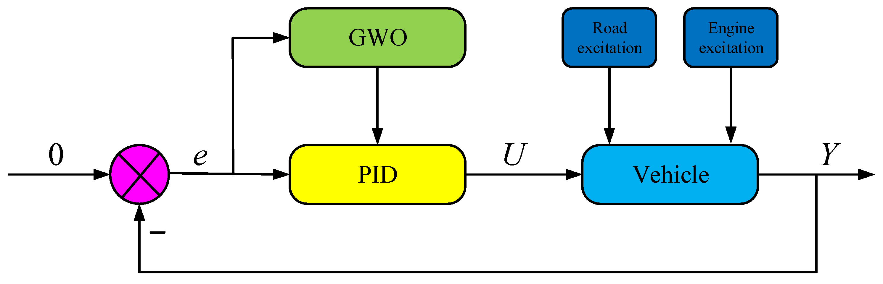
4.1. Logical Architecture

As shown in Figure 3, the fractional-order control-based active suspension system combines the advantages of traditional PID control with the flexibility of fractional-order operators, achieving superior control performance. Under road irregularities and engine vibration excitations, the active suspension system utilizes sensors to collect real-time road profile information and vehicle body vibration data. The GWO algorithm is employed to optimize the parameters of the fractional-order controller offline, ensuring the control strategy achieves optimal performance in both frequency and time domains. This enhances vehicle ride comfort and handling stability.

Tepljakov et al. [115] pioneered the development of FOMCON, an innovative toolbox dedicated to system modeling and control design based on fractional-order calculus. Seamlessly integrated with MATLAB, FOMCON offers a user-friendly interface that standardizes and simplifies the analysis, modeling, and control design of fractional-order systems. The toolbox empowers researchers and engineers to effortlessly construct sophisticated fractional-order models, including fractional-order transfer functions and state-space representations. Moreover, it provides advanced functionalities for designing fractional-order controllers, such as fractional-order PID controllers, thereby facilitating comprehensive research and practical implementation in the domain of fractional-order systems. Interested researchers can explore the toolbox’s comprehensive features and documentation at the official website: https://fomcon.net (accessed on 8 January 2025).

The GWO algorithm can be efficiently implemented in MATLAB through programmatic approaches to address optimization challenges. Drawing inspiration from the sophisticated social hierarchy and hunting behaviors of gray wolves, Mirjalili et al. [116] developed a comprehensive MATLAB implementation of the GWO algorithm. Interested researchers and practitioners can access the original source code and Supplementary Materials through the designated research repository at https://seyedalimirjalili.com/gwo (verified on 8 January 2025).

The suspension dynamics and controller model were established herein, with the detailed SIMULINK block diagram strategically omitted from the main text. Readers seeking comprehensive insights into our simulation framework and algorithmic implementations are directed to the Supplementary Materials, which comprehensively document the FOMCON and GWO computational code [117,118,119,120,121,122].

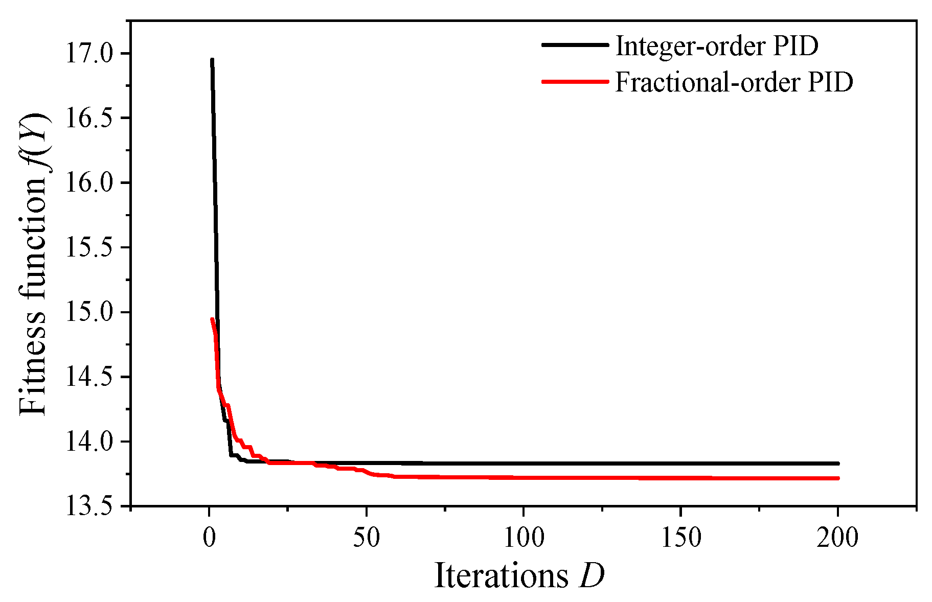
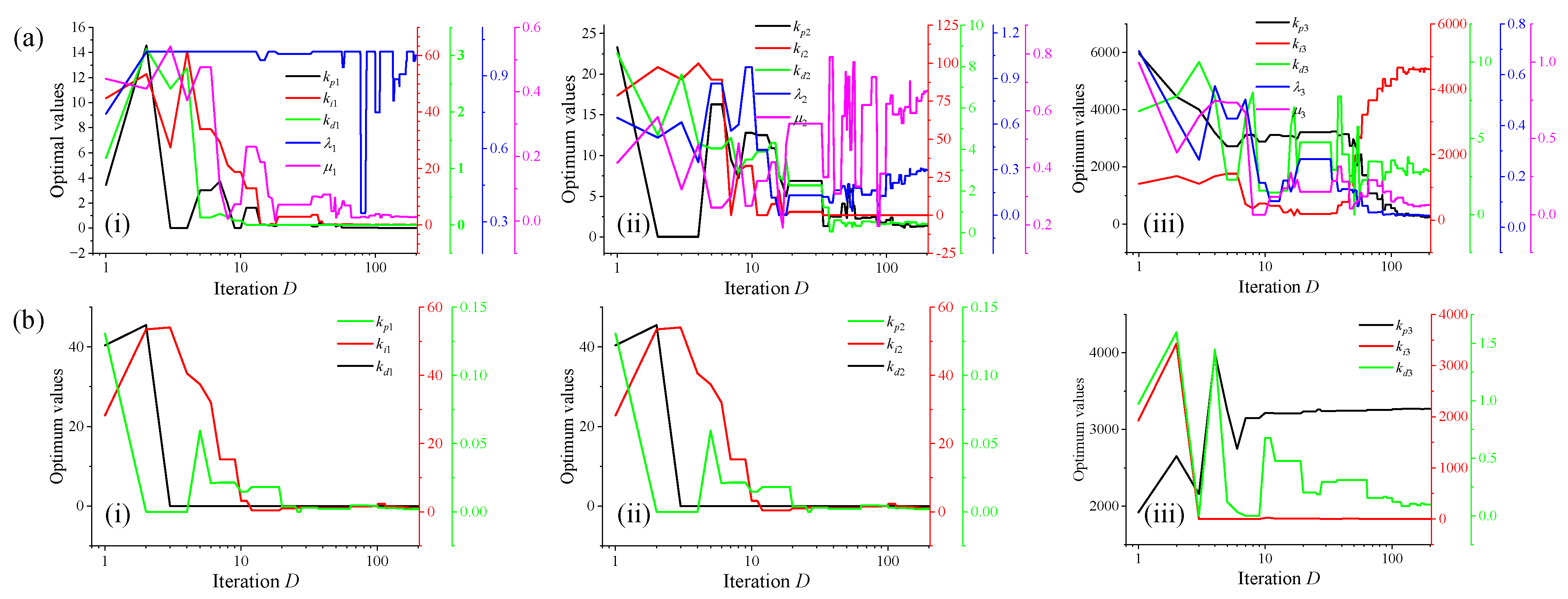
4.2. Parameter Optimization Process

Figure 4 illustrates that the fitness values of both fractional-order PI^λD^μ and integer-order PID controllers exhibit a downward trend as the number of GWO iterations increases. The adaptive performance, measured by the fitness function f(Y), demonstrates a consistent decline for both control strategies as the GWO algorithm progresses through generations. This pattern suggests that both approaches are effectively converging toward optimal solutions, with the fractional-order PID showing potentially smoother adaptation compared to its integer-order counterpart. The gradual decrease in fitness levels across successive GWO generations indicates the algorithm’s effectiveness in refining the control parameters for both PID types. Overall, the data imply that the GWO-based optimization successfully drives both controllers toward higher performance states, highlighting the robustness of the fractional-order PID in maintaining stable convergence.

Figure 5a demonstrates the dynamic adjustments of the integer-order PID controller’s tuning parameters [k_p, k_i, k_d], whereas Figure 5b presents the evolving trends of the FOPID controller’s parameters [k_p, k_i, k_d, λ, μ]. The fluctuations in the PID and FOPID control parameters [k_p, k_i, k_d, λ, μ] do not follow a strictly increasing or decreasing pattern but instead progressively stabilize near the optimal configuration.

Table 9. PID parameters optimized by Gray Wolf Algorithm.

Engine Mountings			Seats			Actuators
PID	I	F	PID	I	F	PID	I	F
kp1	0.0001	0.0198	kp2	0.5066	1.3749	kp3	3269.5862	238.4866
ki1	1.1224	0.1334	k2	2.4706	0.0123	ki3	3.1035	4613.0458
kd1	0.0020	0.0003	kd2	0.0047	0.4002	kd3	0.0976	2.8533
λ1	/	0.9837	λ2	/	0.2986	λ3	/	0.0458
μ1	/	0.0126	μ2	/	0.6701	μ3	/	0.0628

presents optimized PID parameter values for engine mountings, seats, and actuators, including proportional, integral, derivative gains, and fractional-order terms λ and μ.

4.3. Dynamic Processes on C-Level Road Surfaces

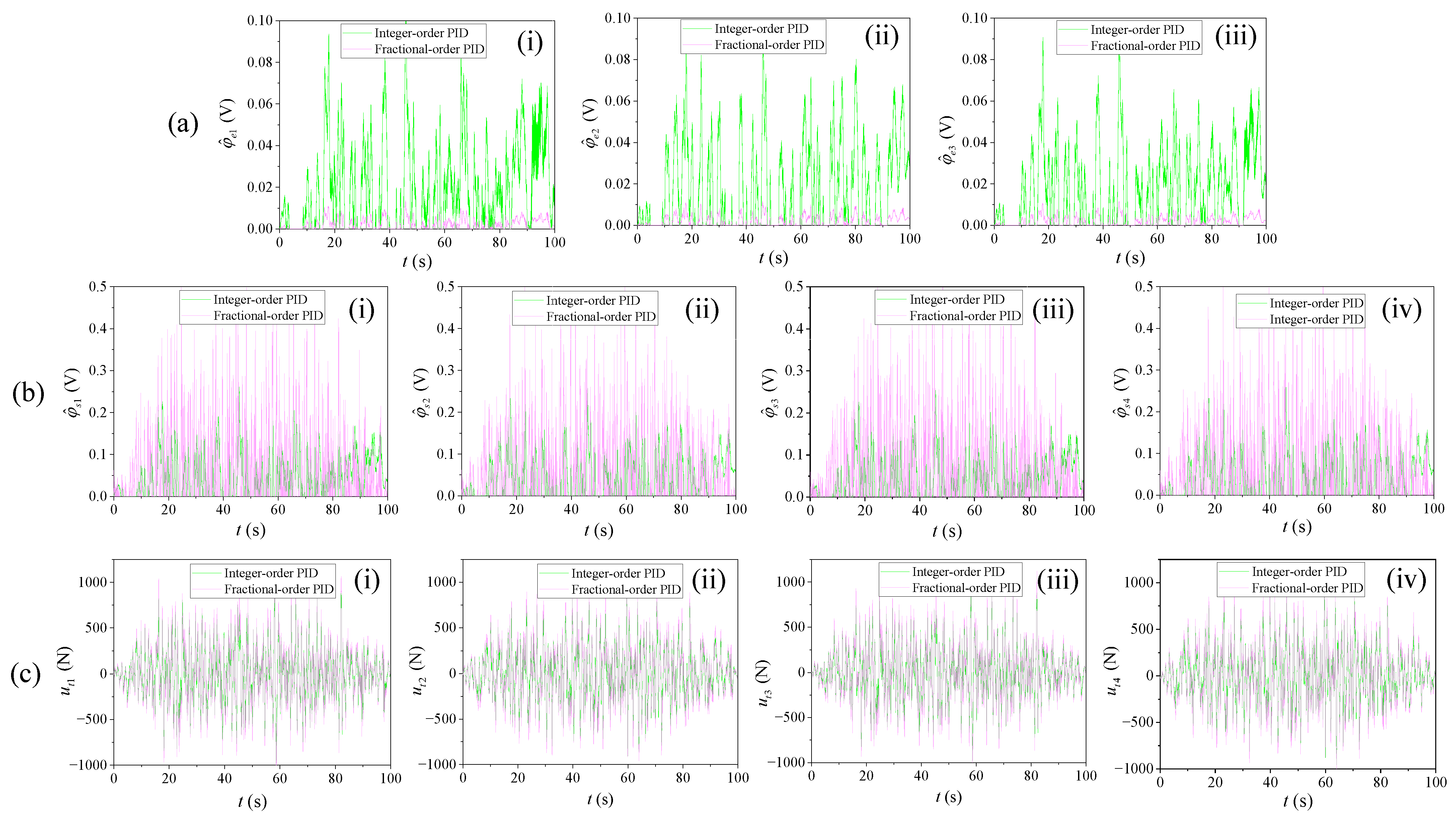
4.3.1. Controller Input

Figure 6 compares the control signals of integer-order PID and FOPID controllers.

Table 10. Statistical analysis and evaluation of control signal values for performance optimization.

PID		${\widehat{\mathit{\phi }}}_{\mathit{e}1}$	${\widehat{\mathit{\phi }}}_{\mathit{e}2}$	${\widehat{\mathit{\phi }}}_{\mathit{e}3}$	${\widehat{\mathit{\phi }}}_{\mathit{s}1}$	${\widehat{\mathit{\phi }}}_{\mathit{s}2}$	${\widehat{\mathit{\phi }}}_{\mathit{s}3}$	${\widehat{\mathit{\phi }}}_{\mathit{s}4}$	ut1	ut2	ut3	ut4
I	RMS	0.0059	0.0035	0.0036	0.0151	0.0105	0.0146	0.0105	133.9700	144.8095	128.7949	146.7290
	AVE	0.0033	0.0018	0.0018	0.0085	0.0057	0.0057	0.0055	9.8852	9.8852	7.4277	7.42767
F	RMS	0.0009	0.0005	0.0005	0.0482	0.0484	0.0488	0.0498	163.2996	180.5513	156.2748	185.4619
	AVE	0.0005	0.0002	0.0003	0.0235	0.0259	0.0242	0.0262	11.76018	−5.0096	8.3197	−8.4500

presents the root mean square (RMS) and average (AVE) values of the control signals. In FOPID, the control signal exhibits both a higher degree of fluctuation and a larger deviation from the mean value, while in integer-order PID control, these variations are comparatively smaller.

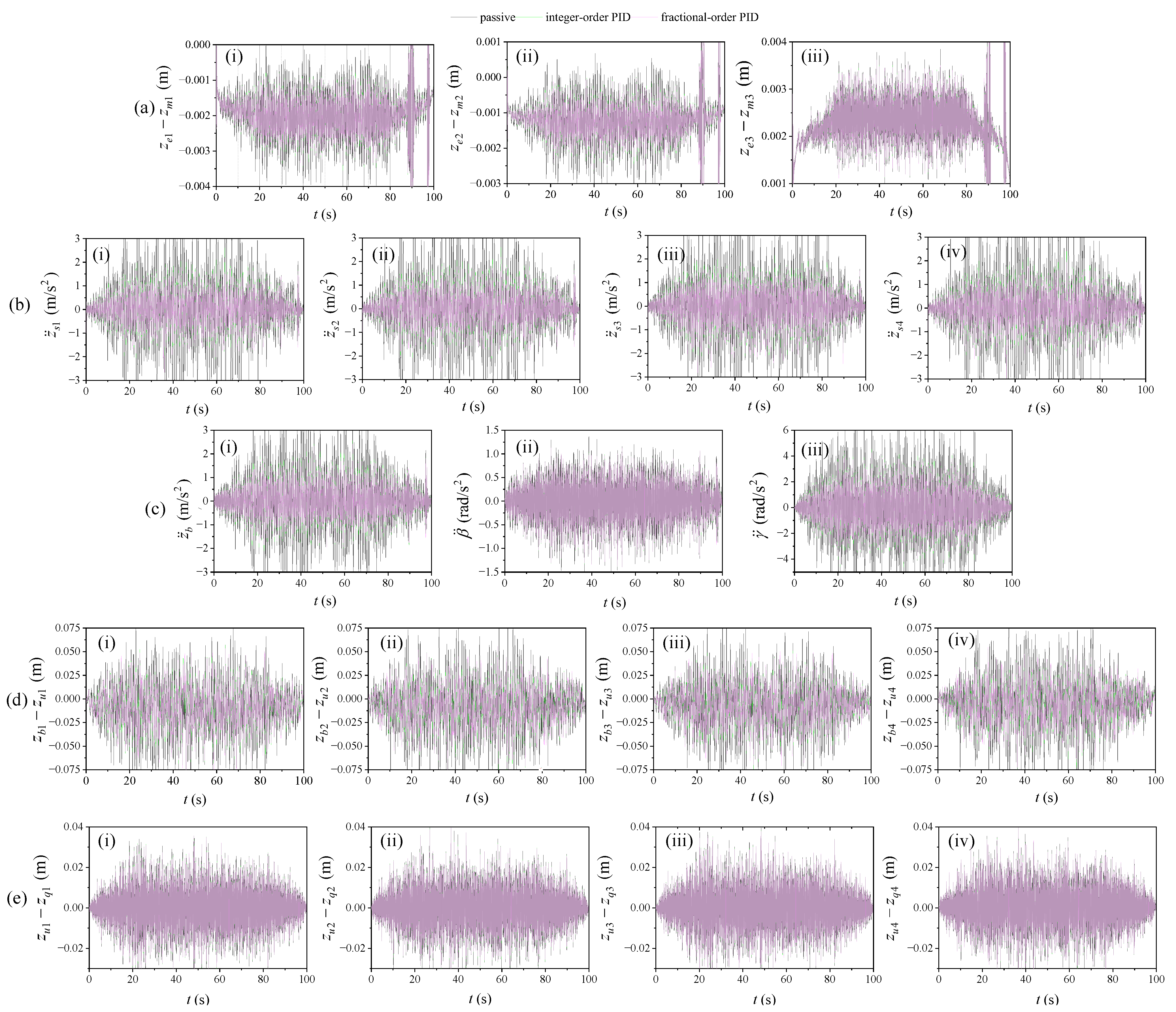
4.3.2. Time-Domain Indicators of Output Response

From Figure 7, it can be observed that the range of variations for the engine mounting displacement is −0.004 to 0.004 m, while the seat displacement acceleration spans from −3.0 to 3.0 m/s². The body displacement acceleration falls within the range of −3.0 to 3.0 m/s², whereas the body pitch angle acceleration is observed to range from −1.5 to 1.5 rad/s². Similarly, the body roll angle acceleration lies between −6.0 and 6.0 rad/s². For the suspension dynamic deflection, the variation range is from −0.075 to 0.075 m, and the tire dynamic displacement is measured to range from −0.04 to 0.04 m. These results quantify the key dynamic responses of the system under analysis, showcasing consistent ranges for the respective parameters, which are critical for evaluating ride comfort, handling stability, and vibration isolation performance.

As illustrated in Figure 7, active-controlled suspension systems demonstrate significant performance enhancements over passive suspension systems in various aspects. Specifically, key metrics such as seat displacement acceleration, vehicle body displacement acceleration, body roll angle acceleration, and suspension deflection all exhibit superior dynamic response capabilities under active control. This indicates that active regulation effectively reduces vehicle vibrations during operation, thereby improving ride comfort and safety. Furthermore, fractional-order PID control displays smoother dynamic characteristics compared to integer-order PID control, with smaller fluctuations in control output and more precise system responses. This highlights the ability of fractional-order PID control to better suppress vibrations and enhance system robustness.

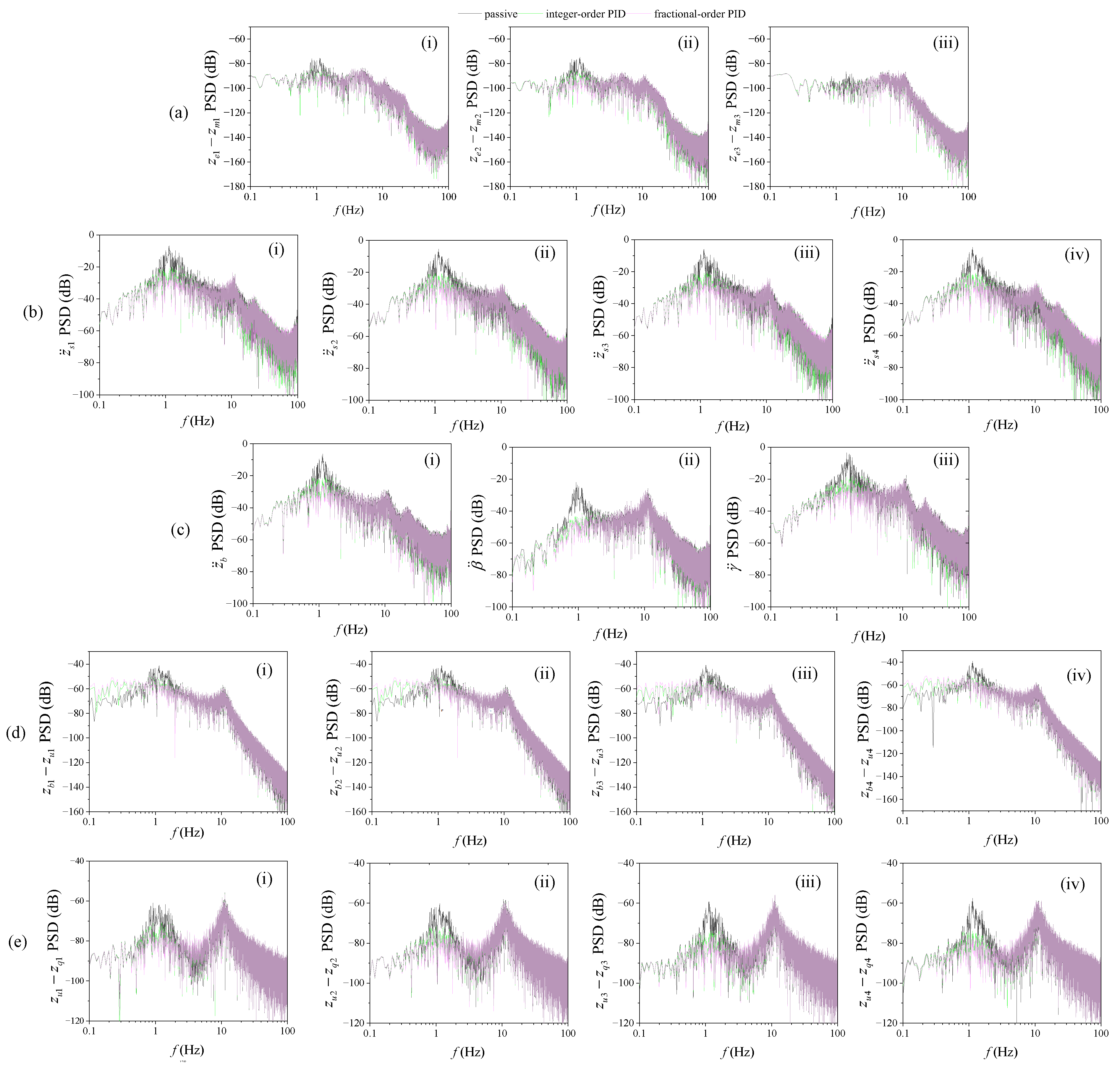
4.3.3. Frequency Domain Comparison of Output Response

Based on Figure 8, the vehicle performance indicators demonstrate two resonance peaks: one at approximately 1 Hz and another at around 10 Hz. The frequency range of 4–8 Hz corresponds to human internal organ resonance, while 8–12.5 Hz significantly affects the spinal system. At frequencies below 3 Hz, humans exhibit greater sensitivity to horizontal vibrations compared to vertical ones.

The power spectral density (PSD) analysis revealed several key characteristics across different vehicle parameters. The engine mount displacement maintained PSD levels below −80 dB throughout the frequency range. Notable peaks were observed in the seat displacement acceleration, with PSD values reaching −10 dB in the 1–2 Hz frequency band, followed by a significant reduction to −30 dB around 1 Hz. Both the body displacement acceleration and body roll angle acceleration exhibited relatively low PSD values, remaining under −20 dB, while the body pitch angle acceleration showed slightly higher values but remained below −30 dB. The suspension dynamic deflection demonstrated moderate PSD levels, not exceeding −50 dB. Regarding the tire dynamic displacement, the PSD values remained consistently below −50 dB, with an interesting characteristic where the PSD magnitude at 10 Hz approximated that at 1 Hz.

In Figure 8, compared to passive suspension, the active control suspension system exhibits a significant decrease in PSD value in the low frequency range. It is worth noting that in the high-frequency region, the difference in PSD values between the two suspension systems is not significant.

4.3.4. RMS Values on Five Different Road Surfaces

Table 11. RMS response values of vehicle states under different suspension controls on various road types.

Road Types		− lg(RMS(Yi))
		RMS(Y1)	RMS(Y2)	RMS(Y3)	RMS(Y4)	RMS(Y5)	RMS(Y6)	RMS(Y7)	RMS(Y8)	RMS(Y9)
A	P	2.6965	2.9008	2.6405	0.4514	0.4687	0.4656	0.4693	0.4553	0.8725
	I	2.6973	2.9026	2.6408	0.6403	0.7358	0.6895	0.7680	0.5948	0.9109
	F	2.6964	2.9017	2.6405	0.6546	0.7559	0.7074	0.7921	0.6030	0.9112
B	P	2.6938	2.8937	2.6398	0.1866	0.1751	0.1805	0.1624	0.2271	0.6986
	I	2.6964	2.9004	2.6401	0.4560	0.5041	0.4680	0.5100	0.4784	0.7461
	F	2.6963	2.9003	2.6402	0.4805	0.5334	0.4944	0.5296	0.4995	0.7462
C	P	2.6821	2.8665	2.6370	−0.1211	−0.1453	−0.1383	−0.1667	−0.5545	0.4454
	I	2.6929	2.8913	2.6380	0.2043	0.2303	0.2006	0.2155	0.2694	0.5074
	F	2.6927	2.8912	2.6378	0.2360	0.2655	0.2314	0.2485	0.3037	0.5076
D	P	2.6440	2.7822	2.6268	−0.4488	−0.4741	−0.4714	−0.5002	−0.3563	0.1561
	I	2.6797	2.8601	2.6305	−0.0718	−0.0536	−0.0753	−0.0647	−0.0031	0.2295
	F	2.6807	2.8629	2.6306	−0.0347	−0.0169	−0.0422	−0.0301	0.0375	0.2296
E	P	2.5292	2.5894	2.5783	−0.7719	−0.7964	−0.7972	−0.8251	−0.6648	−0.1490
	I	2.6317	2.7563	2.5955	−0.3597	−0.3432	−0.3593	−0.3487	−0.2995	−0.0677
	F	2.6351	2.7607	2.5911	−0.3194	−0.2998	−0.3156	−0.3049	−0.2579	−0.0681
Road Types		− lg(RMS(Yi))
		RMS(Y10)	RMS(Y11)	RMS(Y12)	RMS(Y13)	RMS(Y14)	RMS(Y15)	RMS(Y16)	RMS(Y17)	RMS(Y18)
A	P	0.2128	2.1047	2.1373	2.2162	2.1976	2.6890	2.6950	2.6949	2.6921
	I	0.3398	2.2291	2.3219	2.3967	2.4293	2.7150	2.7255	2.7067	2.7099
	F	0.3446	2.3335	2.3239	2.3898	2.4205	2.7176	2.7283	2.7058	2.7092
B	P	0.0237	1.8416	1.8458	1.9006	1.8787	2.3777	2.3819	2.3786	2.3787
	I	0.2000	1.9828	2.0330	2.0828	2.1181	2.4053	2.4136	2.3908	2.3981
	F	0.2088	1.9861	2.0336	2.0766	2.1103	2.4090	2.4172	2.3902	2.3976
C	P	−0.3141	1.5464	−0.3141	1.5465	1.5371	2.0679	2.0622	2.0574	2.0588
	I	−0.0290	1.7034	1.7337	1.7720	1.7970	2.0863	2.0945	2.0698	2.0788
	F	−0.0093	1.7068	1.7344	1.7666	1.7905	2.0907	2.0985	2.0696	2.0786
D	P	−0.6168	1.2431	1.2280	1.2689	1.2396	1.7436	1.7480	1.7423	1.7444
	I	−0.3048	1.4111	1.4326	1.4657	1.4838	1.7724	1.7808	1.7549	1.7646
	F	−0.2816	1.4146	1.4336	1.4606	1.4781	1.7766	1.7849	1.7549	1.7647
E	P	−0.9231	0.9382	0.9210	0.9566	0.9264	1.4349	1.4394	1.4331	1.4353
	I	−0.3018	−0.1141	1.1316	1.1629	1.1765	1.4643	1.4727	1.4460	1.4559
	F	−0.5772	1.1176	1.1328	1.1573	1.1712	1.4687	1.4768.	1.4461	1.4561

details the RMS values of vehicle state output responses under passive suspension (P), integer-order PID control (I), and FOPID control (F) for various road types. It can be observed that the RMS values under passive suspension are significantly higher than the corresponding values under both I and F control. Furthermore, the amplitude of vibrations in the F control state is slightly smaller than that in the I control state, which indicates a relatively more stable driving process. Table 11 shows the −lg(RMS(Y_i)) values of output responses under different road conditions. A larger value indicates smaller vibration response and superior performance.

Table 12. Optimization comparison of vehicle smoothness indicators.

Optimization		RMS(Y1)	RMS(Y2)	RMS(Y3)	RMS(Y4)	RMS(Y5)	RMS(Y6)	RMS(Y7)	RMS(Y8)	RMS(Y9)
Ratio (%)	I/P	0.3	0.65	1.5	35.0	46.0	40.0	50.0	27.0	8.0
	F/P	0.2	0.6	0.5	36.0	48.0	42.0	52.0	30.0	9.0
	F/I	−0.03	0.1	−0.03	3	4.0	4.0	5.0	1.0	1.0
Optimization		RMS(Y10)	RMS(Y11)	RMS(Y12)	RMS(Y13)	RMS(Y14)	RMS(Y15)	RMS(Y16)	RMS(Y17)	RMS(Y18)
Ratio (%)	I/P	25.0	25.0	34.0	33.2	40.0	5.0	5.0	32.0	4.5
	F/P	75.0	26.0	35.0	33.6	41.0	6.0	6.0	30.0	4.4
	F/I	67.0	2.0	2.0	1.3	0.9	1.0	1.0	−0.3	−0.3

presents a comparison of the optimization results for vehicle smoothness indices under different control strategies. Firstly, compared to the passive suspension system, both integer-order PID and FOPID controllers achieve significant optimization results. Specifically, in terms of engine-mounting dynamic displacement (Y₁−Y₃), the optimization is relatively modest; however, for indices such as suspension displacement and dynamic tire load (Y₄−Y₉), both control methods show notable improvements of 25% to 50%. Secondly, when comparing the performance of FOPID to integer-order PID, FOPID slightly outperforms integer-order PID in most indices, with optimization ranges from 0.9% to 67%. In particular, for index Y₁₀, FOPID shows a 67% improvement over integer-order PID, demonstrating a clear advantage. Conversely, for certain indices such as Y₁₇ and Y₁₈, FOPID exhibits a slight decrease relative to integer-order PID, with a reduction of approximately 0.3%. Overall, the FOPID control strategy demonstrates effective control results in optimizing vehicle ride comfort, achieving significant improvements over the passive suspension system and outperforming traditional integer-order PID control in most indices, reflecting its application potential in vehicle suspension control.

From Table 12, it can be observed that the F/P values are generally higher than the I/P values under most road conditions, indicating that FOPID can provide a more significant performance improvement compared to passive suspension. This suggests that FOPID can outperform integer-order PID in certain scenarios, possibly due to its ability to offer more flexible control parameters, thereby better adapting to different road excitations. On the other hand, there may be some instances in Table 12 where F/I values are negative, indicating that under specific road conditions, the performance of integer-order PID may be slightly better than that of FOPID. This may be related to the complexity of tuning FOPID parameters and its insufficient adaptability to certain road excitations.

5. Comparison and Discussion

5.1. Previous Literature

The different control strategies will significantly affect the following indicators, as shown in

Table 13. Comparison and discussion for the optimization quantities.

Studies	Control Algorithm	Optimization Amplitude (%)
		RMS(Y1–3)	RMS(Y4–7)	RMS(Y8)	RMS(Y9)	RMS(Y10)	RMS(Y11–14)	RMS(Y15–18)
Present	PIλDμ	0.3%	46%	30%	9%	75%	34%	2.5%
Dridi et al. [123]	LSTM	/	/	27.9%	/	/	/	/
Nagarkar et al. [124]	FLC	/	/	46.0%	/	/	3.6%	18.7%
Mrazgua et al. [125] FLC	T-S fuzzy	/	/	57.16%	/	/	/	/
Yin et al. [126]	fuzzy PID	/	21.17%	22.00%	21.37%	24.17%	15%	10%
Lee et al. [127]	CDC	/	/	14.53%	/	/	/	/
Shen et al. [128]	sky-hook	/	/	12.8%	/	/	37.3%	8.9%
Nagarkar et al. [129]	NSGA-II algorithm	/	/	47%	/	/	9.2%	35.8%
Wei et al. [130]	fuzzy PID	/	/	59.08%	3.06%	3.54%	11.98%	2.09%
Shen et al. [131]	tructure-immittance approach	/	/	18%	15%	/	/	/
Anandan et al. [132]	PID	/	21%	35%	33%	/	18%	/
Theunissen et al. [133]	e-MPC	/	/	10%	8–21%	8–21%	/	/
Yang et al. [134]	ground-hook	/	/	4.87%	/	/	/	16.19%
Zhang et al. [135]	bridge network	/	/	1.8%	/	/	21.1%	6.3%
Zeng et al. [136]	Neuron PI	/	/	37.2%	45.2%	38.6%	/	/
Jiang et al. [137]	BP-PID	/	/	27.58%	/	/	4.48%	4.17%
Zhou et al. [138]	MPC	/	/	22.38%	/	/	/	/
Wang et al. [139]	pigeon-inspired optimization	/	/	23.1	/	/	6.6%	/
Fossati et al. [140]	NSGA-II	/	21.14%	/	/	/	/	/
Liu et al. [141]	SH-GH	/	/	27.45%	/	/	/	8.53%
Xu et al. [142]	fuzzy	/	/	14.6%	9.6%	5.3%	/	/
Xu et al. [143]	multi-objective optimization	/	/	43.88%	/	/	24.38%	46.46%
Esmaeili et al. [144]	ANFIS	/	/	62%	/	/	5.83%	56.8%
Yang et al. [145]	hybrid-hook damping			26.61%			-6.94%	22.03%
Ho et al. [146]	SMC-NDOB	/	41.5%	/	/	/	/	/
Ning et al. [147]	T-S fuzzy	/	45.5%	/	/	/	/	/
Li et al. [148]	model reference adaptive	/	/	8.70%	/	/	28.26%	18.21%
Xu et al. [149]	LQG	/	/	27.5%	/	/	6.3%	17.6%
Liu et al. [150]	MPC-H∞	/	/	19.4%	/	/	/	9.3%
Wang et al. [151]	DSHIS	/	/	48.17%	56%	/	17.39%	4.35%
Ghorbany et al. [152]	MOPSO	/	/	71%	57%	33%	/	/
Zhang et al. [153]	NESI	/	23.59%	23.97%	27.48%	/	/	/
Alfadhli et al. [154]	feedforward and feedback	/	25%	/	/	/	/	/
Wu et al. [155]	LQR	/	/	58.25%	55.41%	31.39%	/	/
Zhu et al. [156]	VUFC	/	/	21.0%	/	/	/	/
Cao et al. [157]	SOA-PID	/	/	27.6%	27.0%	35.8%	/	/

. A total of seven indicators were analyzed, which are Y_1–3 engine mounting displacement, Y_4–7 seat vertical acceleration in the z-direction, Y₈ vehicle body vertical acceleration in the z-direction, Y₉ pitch angle acceleration, Y₁₀ roll angle acceleration, Y_11-14 suspension dynamic deflection, and Y_15–18 tire dynamic displacement.

Through FOPID control, Y_1–3 was marginally improved by approximately 0.3%. For Y_4–7, Yin et al. [126] optimized RMS by 21.71% using fuzzy PID, while Fossati et al. [140] achieved 21% optimization via PID control. Ho et al. [146] enhanced the indicator by 41.5% through SMC-NDOB control, and Ning et al. [147] optimized it to 44.5% using T-S fuzzy control. Zhang et al. [153] improved 23.59% with NESI control, and Alfadhli et al. [154] realized 25% optimization through feedforward and feedback control. In this study, fractional-order PID control achieved an optimization of 46% for Y_4–7. Fractional-order PID control led to a 30% optimization of Y₈. Nagarkar et al. [124] reached 46% optimization using FLC control strategy, while Mrazgua et al. [125] improved it to 57.16% through fuzzy-PID control. Notably, Wei et al. [130] achieved the highest optimization of 59.8% using a fuzzy-PID control method. The optimization of Y₉ reached 9%. Other researchers have also optimized this indicator through various control strategies. For instance, Yin et al. [126] achieved 21.73% through fuzzy-PID control, Anandan et al. [132] reached 33% via PID control, and Wu et al. [155] elevated the optimization to an impressive 55.41% using LQR control strategy. Regarding Y₁₀, Wei et al. [130] and Yin et al. [126] achieved optimizations of 21.37% and 3.06%, respectively, using fuzzy-PID control. Zeng et al. [136] reached 38.6% optimization with Neuron PI control method, while Cao et al. [157] achieved 35.8% using SOA-PID control. Th FOPID control strategy significantly improved the optimization to 75%. The proposed fractional-order control method optimized Y_11–14 indicators by 34%. Shen et al. [128] achieved 37.3% optimization using sky-hook control method. Researchers like Xu et al. [142], Xu et al. [143], Li et al. [148], and Wang et al. [151] have conducted various optimizations of suspension dynamic deflection through different control strategies. For Y_15–18, this study utilized FOPID control to optimize the indicator by 2.5%. Many researchers have also focused on this aspect. For example, Xu et al. [143] and Esmaeili et al. [144] employed multi-objective optimization and ANFIS control methods to improve Y_15–18 tire dynamic displacement by 55.8% and 22.03%, respectively.

In terms of acceleration control, FOPID control has better performance compared to traditional PID control, as it can respond to system changes faster, reduce overshoot and steady-state error, and improve the control performance of the system. However, in suspension dynamic displacement and tire deflection control, FOPID control exhibits asymmetric effects. In suspension dynamic displacement control, FOPID control may lead to excessive oscillations and instability. On the other hand, in tire deflection control, FOPID control may result in a slow system response, failing to effectively suppress tire deflection. Therefore, in practical applications, it is necessary to choose the appropriate control method based on the specific control object and requirements. For nominal acceleration control, FOPID control is an effective choice that can improve the control performance of the system. However, for suspension dynamic displacement and tire deflection control, it may be necessary to combine other control methods or adjust the parameters of the FOPID controller to achieve better control effects.

5.2. Enhancing the Smoothness of Suspension Through the Utilization of Other Technologies

Enhancing the comfort of suspension systems is one of the key directions in the current automotive industry’s technological innovations. Below, we will explore this topic in detail from four aspects: intelligence, electrification, sharing, and connectivity.

(1) Intelligence: The suspension system can automatically adjust suspension settings based on road conditions and driving habits, improving vehicle comfort and handling. Adaptive suspension systems adjust suspension stiffness and damping in real-time through sensors and control units to cope with different road conditions, providing a smoother riding experience [158]. Predictive suspension uses on-board cameras and sensors to predict the road conditions ahead, adjust suspension settings in advance, and reduce shock and vibration [159]. AI-assisted suspension uses artificial intelligence algorithms to analyze driving data and automatically optimize suspension parameters to achieve optimal comfort and performance [160]. The passenger comfort feedback system adjusts suspension settings to improve comfort by analyzing passenger feedback (such as seat sensor data) [161].

(2) Electrification: With the popularization of electric vehicles, the suspension system needs to achieve better energy management. Electronic control suspension uses electric adjustment mechanisms to replace traditional mechanical structures, improving response speed and adjustment accuracy [162]. The regenerative suspension system has an energy recovery function, which can convert the energy generated by the suspension system when absorbing road impacts into electrical energy and provide more accurate road feedback, enabling the driver to better perceive the dynamic state and road conditions of the vehicle [163]. Intelligent air suspension can adapt to different loads and road conditions by intelligently adjusting the pressure of the air suspension, optimizing comfort and vehicle performance [164].

(3) Sharing: The suspension system needs to adapt to different drivers and changing road conditions. User customized settings allow shared vehicle users to set suspension parameters based on personal preferences, such as softness, hardness, and height [165]. Cloud data sharing and analysis can collect suspension performance data of different users under different road conditions, for optimizing suspension design and adjusting strategies [166]. The real-time road condition feedback system shares the detected road conditions, such as potholes and uneven road surface information, through the network [167]. This information can be utilized by other vehicles to adjust the response of their suspension systems, allowing them to better handle upcoming uneven road surfaces, thereby reducing vibrations and discomfort inside the vehicle.

(4) Networking: Through the Internet of Vehicles technology, the suspension system can receive and analyze external data in real time, such as traffic conditions and weather information. Remote suspension control adjusts the suspension settings remotely via the internet to adapt to the upcoming road conditions or driving modes [168]. Vehicle-to-vehicle communication technology can exchange road condition information and adjust suspension settings to cope with the road conditions ahead [169]. Intelligent transportation systems can obtain traffic flow and road condition information in advance to optimize suspension settings [170,171,172].

6. Conclusions

The investigation implements the gray wolf optimization (GWO) algorithm to optimize fractional-order PID (FOPID) controller parameters for enhanced suspension vibration suppression and ride comfort. Compared with passive suspension systems and integer-order PID controlled active suspension systems, this study verifies the superior performance of FOPID controller in improving suspension indicators through both time-domain and frequency-domain responses. The key findings are as follows:

(1) The optimized FOPID-controlled suspension exhibits significant improvements over passive suspension systems under random road conditions. The root mean square (RMS) of acceleration shows an enhancement exceeding 42%, while suspension dynamic deflection demonstrates improvement above 38%. Engine-mounting dynamic displacement and tire dynamic displacement show optimizations of 4.3% and 2.5%, respectively. In comparison with integer-order PID-controlled suspension systems, the FOPID-controlled suspension achieves a 28% improvement in acceleration RMS and a 2.1% enhancement in suspension dynamic deflection. However, minor decreases of 0.05% and 0.3% are observed in engine-mounting dynamic displacement and tire dynamic displacement optimizations, respectively.

(2) Amplitude-frequency response analyses indicate that the FOPID-controlled active suspension system demonstrates superior acceleration performance under low-frequency disturbances and effectively reduces low-frequency resonance peak values, thereby enhancing operational vehicle stability. The PSD analysis indicates that near the 1 Hz resonance peak, the comfort indices of the PID-controlled suspension decrease by approximately 20 dB compared to the passive suspension. Furthermore, the tire dynamic displacements decreased under low-frequency disturbances, although an increase in deformation was observed at high-frequency resonance peaks.

(3) FOPID control has better performance in acceleration control because it can better handle nonlinear and time-varying systems, improving system stability and robustness. However, the impact of FOPID control on tire dynamic deflections is asymmetric, which may lead to poor responses in some cases.

References

1. Abdelkareem, M.A.A.; Xu, L.; Ali, M.K.A.; Elagouz, A.; Mi, J.; Guo, S.J.; Liu, Y.L.; Zuo, L. Vibration energy harvesting in automotive suspension system: A detailed review. Appl. Energy 2018, 229, 672–699. [Google Scholar]
2. Gao, P.; Zhao, C.; Pan, H.; Fang, L. A Model-Free Fractional-Order Composite Control Strategy for High-Precision Positioning of Permanent Magnet Synchronous Motor. Fractal Fract. 2025, 9, 161. [Google Scholar] [CrossRef]
3. Li, H.Y.; Jing, X.J.; Karimi, H.R. Output-Feedback-Based H Control for Vehicle Suspension Systems with Control Delay. IEEE Trans. Ind. Electron. 2014, 61, 436–446. [Google Scholar]
4. Li, H.Y.; Yu, J.Y.; Hilton, C.; Liu, H.H. Adaptive Sliding-Mode Control for Nonlinear Active Suspension Vehicle Systems Using T-S Fuzzy Approach. IEEE Trans. Ind. Electron. 2013, 60, 3328–3338. [Google Scholar]
5. Sun, W.C.; Zhao, Z.L.; Gao, H.J. Saturated Adaptive Robust Control for Active Suspension Systems. IEEE Trans. Ind. Electron. 2013, 60, 3889–3896. [Google Scholar]
6. Wang, H.; Jian, H.; Huang, J.; Lan, Y. Fractional-Order MFAC with Application to DC Motor Speed Control System. Mathematics 2025, 13, 610. [Google Scholar] [CrossRef]
7. Ferhath, A.A.; Kasi, K. A Review on Various Control Strategies and Algorithms in Vehicle Suspension Systems. Int. J. Automot. Mech. Eng. 2023, 20, 10720–10735. [Google Scholar]
8. Ezeta, J.H.; Mandow, A.; Cerezo, A.G. Active and Semi-active Suspension Systems: A Review. Rev. Iberoam. Autom. Inform. 2013, 10, 121–132. [Google Scholar]
9. Liu, C.N.; Chen, L.; Lee, H.P.; Yang, Y.; Zhang, X.L. Generalized Skyhook-Groundhook Hybrid Strategy and Control on Vehicle Suspension. IEEE Trans. Veh. Technol. 2023, 72, 1689–1700. [Google Scholar]
10. Zhang, J.M.; Liu, J.; Liu, B.L.; Li, M. Fractional Order PID Control Based on Ball Screw Energy Regenerative Active Suspension. Actuators 2022, 11, 189. [Google Scholar] [CrossRef]
11. Guan, Q.H.; Du, X.; Wen, Z.F.; Liang, S.L.; Chi, M.R. Vibration characteristics of bogie hunting motion based on root loci curves. Acta Mech. Sin.-PRC 2022, 38, 521447. [Google Scholar]
12. Zhu, H.M.; Yang, Z.B.; Sun, X.D.; Wang, D.; Chen, X. Rotor Vibration Control of a Bearingless Induction Motor Based on Unbalanced Force Feed-Forward Compensation and Current Compensation. IEEE Access 2020, 8, 12988–12998. [Google Scholar]
13. Hoyle, J.B. Modelling the static stiffness and dynamic frequency response characteristics of a leaf spring truck suspension. Proc. Inst. Mech. Eng. Part D J. Automob. Eng. 2004, 218, 259–278. [Google Scholar]
14. Floreán-Aquino, K.H.; Arias-Montiel, M.; Linares-Flores, J.; Mendoza-Larios, J.G.; Cabrera-Amado, A. Modern Semi-Active Control Schemes for a Suspension with MR Actuator for Vibration Attenuation. Actuators 2021, 10, 22. [Google Scholar] [CrossRef]
15. Liu, C.C.; Ren, C.B.; Liu, L. Optimal Control for Cubic Strongly Nonlinear Vibration of Automobile Suspension. J. Low Freq. Noise Vib. Act. Control 2014, 33, 233–243. [Google Scholar]
16. Zribi, M.; Karkoub, M. Robust control of a car suspension system using magnetorheological dampers. J. Vib. Control 2004, 10, 507–524. [Google Scholar]
17. Koch, G.; Kloiber, T. Driving State Adaptive Control of an Active Vehicle Suspension System. IEEE Trans. Control Syst. Technol. 2014, 22, 44–57. [Google Scholar]
18. Dou, G.W.; Yu, W.H.; Li, Z.X.; Khajepour, A.; Tan, S.Q. Sliding Mode Control of Laterally Interconnected Air Suspensions. Appl. Sci. 2020, 10, 4320. [Google Scholar] [CrossRef]
19. Li, Y.; Dong, W.; Zheng, T.; Wang, Y.; Li, X. Scene-Adaptive Loader Trajectory Planning and Tracking Control. Sensors 2025, 25, 1135. [Google Scholar] [CrossRef]
20. Fan, Y.; Ren, H.B.; Zhao, Y.Z. Observer design based on nonlinear suspension model with unscented Kalman filter. J. Vibroeng. 2015, 17, 3844–3855. [Google Scholar]
21. Buckner, G.D.; Schuetze, K.T.; Beno, J.H. Intelligent feedback linearization for active vehicle suspension control. J. Dyn. Syst. Meas. Control 2001, 123, 727–733. [Google Scholar]
22. Xie, Z.C.; You, W.; Wong, P.K.; Li, W.F.; Zhao, J. Fuzzy robust non-fragile control for nonlinear active suspension systems with time varying actuator delay. Proc. Inst. Mech. Eng. Part D J. Automob. Eng. 2024, 238, 46–62. [Google Scholar]
23. Su, L.; Mao, Y.Y.; Zhang, Y. Deviation Sequence Neural Network Control for Path Tracking of Autonomous Vehicles. Actuators 2024, 13, 101. [Google Scholar] [CrossRef]
24. Lin, X.Y.; Li, K.L.; Wang, L.M. A driving-style-oriented adaptive control strategy based PSO-fuzzy expert algorithm for a plug-in hybrid electric vehicle. Expert Syst. Appl. 2022, 201, 117236. [Google Scholar]
25. Tian, Y.T.; Huang, K.; Cao, X.H.; Liu, Y.L.; Ji, X.W. A hierarchical adaptive control framework of path tracking and roll stability for intelligent heavy vehicle with MPC. Proc. Inst. Mech. Eng. Part D J. Automob. Eng. 2020, 234, 2933–2946. [Google Scholar]
26. Liu, H.; Kiumarsi, B.; Kartal, Y.; Koru, A.T.; Modares, H.; Lewis, F.L. Reinforcement Learning Applications in Unmanned Vehicle Control: A Comprehensive Overview. Unmanned Syst. 2023, 11, 17–26. [Google Scholar]
27. Sun, X.Q.; Wu, P.C.; Cai, Y.F.; Wang, S.H.; Chen, L. Piecewise affine modeling and hybrid optimal control of intelligent vehicle longitudinal dynamics for velocity regulation. Mech. Syst. Signal Process. 2022, 162, 108089. [Google Scholar]
28. Shi, P.C.; Li, L.; Yang, A.X. Intelligent Vehicle Path Tracking Control Based on Improved MPC and Hybrid PID. IEEE Access 2022, 10, 94133–94144. [Google Scholar]
29. Sun, X.Q.; Zhang, H.Z.; Cai, Y.F.; Wang, S.H.; Chen, L. Hybrid modeling and predictive control of intelligent vehicle longitudinal velocity considering nonlinear tire dynamics. Nonlinear Dynam. 2019, 97, 1051–1066. [Google Scholar]
30. Zhang, R.H.; Wu, N.; Wang, Z.H.; Li, K.N.; Song, Z.M.; Chang, Z.T.; Chen, X.; Yu, F. Constrained hybrid optimal model predictive control for intelligent electric vehicle adaptive cruise using energy storage management strategy. J. Energy Storage 2023, 65, 107383. [Google Scholar]
31. Murphey, Y.L.; Park, J.; Chen, Z.H.; Kuang, M.L.; Masrur, M.A.; Phillips, A.M. Intelligent Hybrid Vehicle Power Control-Part I: Machine Learning of Optimal Vehicle Power. IEEE Trans. Veh. Technol. 2012, 61, 3519–3530. [Google Scholar]
32. Zhang, L.A.; Wang, Y.Z.; Zhu, H.Z. Theory and Experiment of Cooperative Control at Multi-Intersections in Intelligent Connected Vehicle Environment: Review and Perspectives. Sustainability 2022, 14, 1542. [Google Scholar] [CrossRef]
33. Zhang, H.; Xi, Z. New Predefined Time Sliding Mode Control Scheme for Multi-Switch Combination–Combination Synchronization of Fractional-Order Hyperchaotic Systems. Fractal Fract. 2025, 9, 147. [Google Scholar] [CrossRef]
34. Nodland, D.; Zargarzadeh, H.; Jagannathan, S. Neural Network-Based Optimal Adaptive Output Feedback Control of a Helicopter UAV. IEEE Trans. Neural Networks Learn. Syst. 2013, 24, 1061–1073. [Google Scholar]
35. Tang, X.Z.; Shi, L.F.; Wang, B.; Cheng, A.Q. Weight Adaptive Path Tracking Control for Autonomous Vehicles Based on PSO-BP Neural Network. Sensors 2023, 23, 412. [Google Scholar]
36. Liu, B.; Wei, X.D.; Sun, C.; Wang, B.; Huo, W.W. A controllable neural network-based method for optimal energy management of fuel cell hybrid electric vehicles. Int. J. Hydrogen Energy 2024, 55, 1371–1382. [Google Scholar]
37. Quintero-Manríquez, E.; Sanchez, E.N.; Antonio-Toledo, M.E.; Muñoz, F. Neural control of an induction motor with regenerative braking as electric vehicle architecture. Eng. Appl. Artif. Intell. 2021, 104, 104275. [Google Scholar]
38. Lin, Y.; Tang, P.; Zhang, W.J.; Yu, Q. Artificial neural network modelling of driver handling behaviour in a driver-vehicle-environment system. Int. J. Vehicle Des. 2005, 37, 24–45. [Google Scholar]
39. Chen, X.; Zhou, Y. Modelling and Analysis of Automobile Vibration System Based on Fuzzy Theory under Different Road Excitation Information. Complexity 2018, 2018, 2381568. [Google Scholar]
40. Ji, G.; Zhang, L.; Shan, M.; Zhang, J. Enhanced variable universe fuzzy PID control of the active suspension based on expansion factor parameters adaption and genetic algorithm. Eng. Res. Express 2023, 5, 035007. [Google Scholar]
41. Chiou, J.S.; Tsai, S.H.; Liu, M.T. A PSO-based adaptive fuzzy PID-controllers. Simul. Model. Pract. Theory 2012, 26, 49–59. [Google Scholar] [CrossRef]
42. Wang, J.; Lv, K.; Wang, H.; Guo, S.; Wang, J. Research on nonlinear model and fuzzy fractional order PIλDμ control of air suspension system. J. Low Freq. Noise Vib. Act. Control 2022, 41, 712–731. [Google Scholar] [CrossRef]
43. Bashir, A.O.; Rui, X.T.; Zhang, J.S. Ride Comfort Improvement of a Semi-active Vehicle Suspension Based on Hybrid Fuzzy and Fuzzy-PID Controller. Stud. Inform. Control 2019, 28, 421–430. [Google Scholar] [CrossRef]
44. Shouran, M.; Alenezi, M.; Muftah, M.N.; Almarimi, A.; Abdallah, A.; Massoud, J. A Novel AVR System Utilizing Fuzzy PIDF Enriched by FOPD Controller Optimized via PSO and Sand Cat Swarm Optimization Algorithms. Energies 2025, 18, 1337. [Google Scholar] [CrossRef]
45. Soukkou, A.; Soukkou, Y.; Haddad, S.; Benghanem, M.; Rabhi, A. Review, design, stabilization and synchronization of fractional-order energy resources demand-supply hyperchaotic systems using fractional-order PD-based feedback control scheme. Arch. Control Sci. 2023, 33, 539–563. [Google Scholar]
46. Fu, M.W.; Shen, D.F.; Zhao, G.; Shang, G.F.; Bai, S.W.; Li, X.F.; Hao, Z.M. Integrated sliding mode intelligent fractional-order backstepping control of warp tension based on fixed-time extended state observer. Text. Res. J. 2023, 93, 3368–3381. [Google Scholar] [CrossRef]
47. Muresan, C.I.; Birs, I.R.; Dulf, E.H.; Copot, D.; Miclea, L. A Review of Recent Advances in Fractional-Order Sensing and Filtering Techniques. Sensors 2021, 21, 5920. [Google Scholar] [CrossRef]
48. Shao, K.; Xia, W.; Zhu, Y.; Sun, C.; Liu, Y. Research on UAV Trajectory Tracking Control System Based on Feedback Linearization Control–Fractional Order Model Predictive Control. Processes 2025, 13, 801. [Google Scholar] [CrossRef]
49. Luo, Y.; Chen, Y.Q.; Pi, Y.G. Tuning fractional order proportional integral controllers for fractional order systems. J. Process Control 2010, 20, 823–831. [Google Scholar] [CrossRef]
50. Miao, Y.; Gao, Z.; Yang, C. Adaptive Fractional-order Unscented Kalman Filters for Nonlinear Fractional-order Systems. Int. J. Control Autom. 2022, 20, 283–1293. [Google Scholar] [CrossRef]
51. Adhikary, A.; Sen, S.; Biswas, K. Practical Realization of Tunable Fractional Order Parallel Resonator and Fractional Order Filters. IEEE Trans. Circuits Syst. I Regul. Pap. 2016, 63, 1142–1151. [Google Scholar] [CrossRef]
52. Zhao, C.N.; Jiang, M.R.; Huang, Y.Q. Formal Verification of Fractional-Order PID Control Systems Using Higher-Order Logic. Fractal Fract. 2022, 6, 485. [Google Scholar] [CrossRef]
53. Zou, Q.; Jin, Q.B.; Zhang, R.D. Design of fractional order predictive functional control for fractional industrial processes. Chemom. Intell. Lab. 2016, 152, 34–41. [Google Scholar] [CrossRef]
54. Vinagre, B.M.; Petrás, I.; Podlubny, I.; Chen, Y.Q. Using fractional order adjustment rules and fractional order reference models in model-reference adaptive control. Nonlinear Dynam. 2002, 29, 269–279. [Google Scholar] [CrossRef]
55. Bialic, G.; Stanislawski, R. On the Linear-Quadratic-Gaussian Control Strategy for Fractional-Order Systems. Fractal Fract. 2022, 6, 248. [Google Scholar] [CrossRef]
56. Bingi, K.; Prusty, B.R.; Singh, A.P. A Review on Fractional-Order Modelling and Control of Robotic Manipulators. Fractal Fract. 2023, 7, 77. [Google Scholar] [CrossRef]
57. Viola, J.; Chen, Y.Q. A Fractional-Order On-Line Self Optimizing Control Framework and a Benchmark Control System Accelerated Using Fractional-Order Stochasticity. Fractal Fract. 2022, 6, 549. [Google Scholar] [CrossRef]
58. Kumar, N.; Mehra, M. Generalized fractional-order Legendre wavelet method for two dimensional distributed order fractional optimal control problem. J. Vib. Control 2024, 30, 1690–1705. [Google Scholar] [CrossRef]
59. Tavakoli-Kakhki, M.; Haeri, M.; Tavazoei, M.S. Study on Control Input Energy Efficiency of Fractional Order Control Systems. IEEE J. Emerg. Sel. Top. Circuits Syst. 2013, 3, 475–482. [Google Scholar]
60. Ding, Y.X.; Luo, Y.; Chen, Y.Q. Dynamic Feedforward-Based Fractional Order Impedance Control for Robot Manipulator. Fractal Fract. 2023, 7, 52. [Google Scholar] [CrossRef]
61. Delavari, H.; Heydarinejad, H. Fractional-Order Backstepping Sliding-Mode Control Based on Fractional-Order Nonlinear Disturbance Observer. J. Comput. Nonlinear Dyn. 2018, 13, 111009. [Google Scholar]
62. Pan, H.H.; Sun, W.C. Nonlinear Output Feedback Finite-Time Control for Vehicle Active Suspension Systems. IEEE Trans. Ind. Inform. 2019, 15, 2073–2082. [Google Scholar] [CrossRef]
63. Sun, W.C.; Gao, H.J.; Kaynak, O. Vibration Isolation for Active Suspensions with Performance Constraints and Actuator Saturation. IEEE-ASME Trans. Mech. 2015, 20, 675–683. [Google Scholar]
64. Wen, S.P.; Chen, M.Z.Q.; Zeng, Z.G.; Yu, X.H.; Huang, T.W. Fuzzy Control for Uncertain Vehicle Active Suspension Systems via Dynamic Sliding-Mode Approach. IEEE Trans. Syst. Man Cybern. Syst. 2018, 47, 24–32. [Google Scholar] [CrossRef]
65. Jin, X.J.; Wang, J.D.; He, X.K.; Yan, Z.Y.; Xu, L.W.; Wei, C.F.; Yin, G.D. Improving Vibration Performance of Electric Vehicles Based on In-Wheel Motor-Active Suspension System via Robust Finite Frequency Control. IEEE Trans. Intell. Transp. 2023, 24, 1631–1643. [Google Scholar]
66. Gu, Z.; Sun, X.; Lam, H.K.; Yue, D.; Xie, X.P. Event-Based Secure Control of T-S Fuzzy-Based 5-DOF Active Semivehicle Suspension Systems Subject to DoS Attacks. IEEE Trans. Fuzzy Syst. 2022, 30, 2032–2043. [Google Scholar] [CrossRef]
67. Liu, L.; Li, X.S.; Liu, Y.J.; Tong, S.C. Neural network based adaptive event trigger control for a class of electromagnetic suspension systems. Control Eng. Pract. 2021, 106, 104675. [Google Scholar]
68. Shi, Z.Q.; Cao, R.L.; Zhang, S.S.; Guo, J.; Yu, S.Y.; Chen, H. Active suspension H/generalized H2 static output feedback control. J. Vib. Control 2023, 30, 5183–5195. [Google Scholar]
69. Zhao, Y.L.; Wang, X. A Review of Low-Frequency Active Vibration Control of Seat Suspension Systems. Appl. Sci. 2019, 9, 3326. [Google Scholar] [CrossRef]
70. Go, C.G.; Sui, C.H.; Shih, M.H.; Sung, W.P. A Linearization Model for the Displacement Dependent Semi-active Hydraulic Damper. J. Vib. Control 2010, 16, 2195–2214. [Google Scholar]
71. Wang, W.L.; Yu, D.S.; Xu, R. Prediction of the in-service performance of a railway hydraulic damper. Proc. Inst. Mech. Eng. Part F J. Rail Rapid Transit 2017, 231, 19–32. [Google Scholar]
72. Farjoud, A.; Ahmadian, M.; Craft, M.; Burke, W. Nonlinear modeling and experimental characterization of hydraulic dampers: Effects of shim stack and orifice parameters on damper performance. Nonlinear Dynam. 2012, 67, 1437–1456. [Google Scholar]
73. Habib, G.; Detroux, T.; Viguié, R.; Kerschen, G. Nonlinear generalization of Den Hartog’s equal-peak method. Mech. Syst. Signal Process. 2015, 52–53, 17–28. [Google Scholar]
74. Habib, G.; Kádár, F.; Papp, B. Impulsive vibration mitigation through a nonlinear tuned vibration absorber. Nonlinear Dynam. 2019, 98, 2115–2130. [Google Scholar]
75. Gao, J.; Wu, F.Q.; Li, Z.X. Study on the Effect of Stiffness Matching of Anti-Roll Bar in Front and Rear of Vehicle on the Handling Stability. Int. J. Automot. Technol. 2021, 2, 185–199. [Google Scholar] [CrossRef]
76. Nguyen, D.N.; Le, M.P.; Nguyen, T.A.; Hoang, T.B.; Tran, T.T.H.; Dang, N.D. Enhancing the Stability and Safety of Vehicle When Steering by Using the Active Stabilizer Bar. Math. Probl. Eng. 2022, 2022, 5617167. [Google Scholar]
77. Adams, S.G.; Bertsch, F.M.; Shaw, K.A.; MacDonald, N.C. Independent tuning of linear and nonlinear stiffness coefficients. J. Microelectromech. Syst. 1998, 7, 172–180. [Google Scholar]
78. Aghasizade, S.; Mirzaei, M.; Rafatnia, S. Novel constrained control of active suspension system integrated with anti-lock braking system based on 14-degree of freedom vehicle model. Proc. Inst. Mech. Eng. Part K J. Multi-Body Dyn. 2018, 232, 501–520. [Google Scholar] [CrossRef]
79. Vaddi, P.K.R.; Kumar, C.S. A non-linear vehicle dynamics model for accurate representation of suspension kinematics. Proc. Inst. Mech. Eng. Part C J. Mech. Eng. Sci. 2015, 229, 1002–1014. [Google Scholar]
80. Hosen, M.A.; Chowdhury, M.S.H. Accurate approximations of the nonlinear vibration of couple-mass-spring systems with linear and nonlinear stiffnesses. J. Low Freq. Noise Vib. Act. Control 2021, 40, 1072–1090. [Google Scholar]
81. Zhang, N.; Zhao, Q. Back-Stepping Sliding Mode Controller Design for Vehicle Seat Vibration Suppression Using Magnetorheological Damper. J. Vib. Eng. Technol. 2021, 9, 1885–1902. [Google Scholar]
82. Zhang, L.X.; Zhao, C.M.; Qian, F.; Dhupia, J.S.; Wu, M.L. An Active Control with a Magnetorheological Damper for Ambient Vibration. Machines 2022, 10, 82. [Google Scholar] [CrossRef]
83. Woo, S.; Shin, D. A Double Sky-Hook Algorithm for Improving Road-Holding Property in Semi-Active Suspension Systems for Application to In-Wheel Motor. Appl. Sci. 2021, 11, 8912. [Google Scholar] [CrossRef]
84. Hui, Y.; Kang, H.J.; Law, S.S.; Hua, X.G. Effect of cut-off order of nonlinear stiffness on the dynamics of a sectional suspension bridge model. Eng. Struct. 2019, 185, 377–391. [Google Scholar]
85. Ahamed, R.; Rashid, M.M.; Ferdaus, M.M.; Yusuf, H.B. Modelling and performance evaluation of energy harvesting linear magnetorheological (MR) damper. J. Low Freq. Noise Vib. Act. Control 2017, 36, 177–192. [Google Scholar]
86. Yan, Z.Y.; Li, G.; Luo, J.; Zeng, J.S.; Zhang, W.H.; Wang, Y.Y.; Yang, W.J.; Ma, G.T. Vibration control of superconducting electro-dynamic suspension train with electromagnetic and sky-hook damping methods. Vehicle Syst. Dyn. 2022, 60, 3375–3397. [Google Scholar]
87. Ning, D.H.; Sun, S.S.; Du, H.P.; Li, W.H.; Zhang, N.; Zheng, M.Y.; Luo, L. An electromagnetic variable inertance device for seat suspension vibration control. Mech. Syst. Signal Process. 2019, 133, 106259. [Google Scholar]
88. Shangguan, W.B.; Shui, Y.J.; Rakheja, S. Kineto-dynamic design optimisation for vehicle-specific seat-suspension systems. Vehicle Syst. Dyn. 2017, 55, 1643–1664. [Google Scholar]
89. Jeon, J.; Han, Y.M.; Lee, D.Y.; Choi, S.B. Vibration control of the engine body of a vehicle utilizing the magnetorheological roll mount and the piezostack right-hand mount. Proc. Inst. Mech. Eng. Part D J. Automob. Eng. 2013, 227, 1562–1577. [Google Scholar]
90. Choi, S.B.; Song, H.J.; Lee, H.H.; Lim, S.C.; Kim, J.H.; Choi, H.J. Vibration control of a passenger vehicle featuring magnetorheological engine mounts. Int. J. Veh. Des. 2003, 33, 2–16. [Google Scholar]
91. Li, R.; Chen, W.M.; Liao, C.R. Hierarchical fuzzy control for engine isolation via magnetorheological fluid mounts. Proc. Inst. Mech. Eng. Part D J. Automob. Eng. 2010, 224, 175–187. [Google Scholar] [CrossRef]
92. Müller, P.C.; Popp, K.; Schiehlen, W.O. Berechnungsverfahren für stochastische Fahrzeugschwingungen. Arch. Appl. Mech. 1980, 49, 235–254. [Google Scholar]
93. Si, Z.Y.; Bai, X.X.; Qian, L.J.; Chen, P. Principle and Control of Active Engine Mount Based on Magnetostrictive Actuator. Chin. J. Mech.-Eng. 2022, 35, 146. [Google Scholar] [CrossRef]
94. Jin, Y.F.; Luo, X. Stochastic optimal active control of a half-car nonlinear suspension under random road excitation. Nonlinear Dynam. 2013, 72, 185–195. [Google Scholar] [CrossRef]
95. Ren, J.P.; Zhang, H.J.; Hao, H.R.; Zhou, D.; Wang, J.W.; Zhao, W.C. Modelling and simulation of suspension system based on topological structure. Proc. Inst. Mech. Eng. Part D J. Automob. Eng. 2024, 239, 1142–1154. [Google Scholar] [CrossRef]
96. Liu, Y.J.; Cui, D.W. Collaborative model analysis on ride comfort and handling stability. J. Vibroeng. 2019, 21, 1724–1737. [Google Scholar] [CrossRef]
97. Yuen, K.V.; Guo, H.Z.; Mu, H.Q. Bayesian Vehicle Load Estimation, Vehicle Position Tracking, and Structural Identification for Bridges with Strain Measurement. Struct. Control Health Monit. 2023, 2023, 4752776. [Google Scholar] [CrossRef]
98. Liu, D.W.; Jiang, R.C.; Wang, S.; Chen, H.M.; Yang, X. Study on Impact Characteristic of Speed Control Hump on Heavy Vehicle. J. Vib. Eng. Technol. 2015, 3, 601–614. [Google Scholar]
99. Wang, X.L.; Cheng, Z.; Ma, N.L. Road Recognition Based on Vehicle Vibration Signal and Comfortable Speed Strategy Formulation Using ISA Algorithm. Sensors 2022, 22, 6682. [Google Scholar] [CrossRef]
100. Ma, B.; Li, P.H.; Guo, X.; Zhao, H.X.; Chen, Y. A Novel Online Prediction Method for Vehicle Velocity and Road Gradient Based on a Flexible-Structure Auto-Regressive Integrated Moving Average Model. Sustainability 2023, 15, 15639. [Google Scholar] [CrossRef]
101. Cao, Y.; Cao, J.Y.; Yu, F.; Luo, Z. A new vehicle path-following strategy of the steering driver model using general predictive control method. Proc. Inst. Mech. Eng. Part C J. Mech. Eng. Sci. 2019, 232, 4578–4587. [Google Scholar] [CrossRef]
102. Attia, T.; Vamvoudakis, K.G.; Kochersberger, K.; Bird, J.; Furukawa, T. Simultaneous dynamic system estimation and optimal control of vehicle active suspension. Vehicle Syst. Dyn. 2019, 57, 1467–1493. [Google Scholar]
103. Li, W.; Liang, H.J.; Xia, D.B.; Fu, J.; Yu, M. Explicit model predictive control of magnetorheological suspension for all-terrain vehicles with road preview. Smart Mater. Struct. 2024, 33, 035037. [Google Scholar]
104. Ammanagi, S.; Manohar, C.S. Optimal cross-spectrum of road loads on vehicles: Theory and experiments. J. Vib. Control 2016, 22, 4012–4024. [Google Scholar] [CrossRef]
105. Bogsjö, K. Coherence of road roughness in left and right wheel-path. Veh. Syst. Dyn. 2008, 46, 599–609. [Google Scholar]
106. Colombaroni, C.; Fusco, G.; Isaenko, N. Coherence analysis of road safe speed and driving behaviour from floating car data. IET Intell. Transp. Syst. 2020, 14, 985–992. [Google Scholar]
107. Aguila-Camacho, N.; Duarte-Mermoud, M.A.; Gallegos, J.A. Lyapunov functions for fractional order systems. Commun. Nonlinear Sci. 2014, 19, 2951–2957. [Google Scholar] [CrossRef]
108. Duarte-Mermoud, M.A.; Aguila-Camacho, N.; Gallegos, J.A.; Castro-Linares, R. Using general quadratic Lyapunov functions to prove Lyapunov uniform stability for fractional order systems. Commun. Nonlinear Sci. 2015, 22, 650–659. [Google Scholar] [CrossRef]
109. Rakkiyappan, R.; Cao, J.D.; Velmurugan, G. Existence and Uniform Stability Analysis of Fractional-Order Complex-Valued Neural Networks With Time Delays. IEEE Trans. Neural Netw. Learn. Syst. 2015, 26, 84–97. [Google Scholar]
110. Yang, Q.; Chen, D.L.; Zhao, T.B.; Chen, Y.Q. Fractional calculus in image processing: A review. Fract. Calc. Appl. Anal. 2016, 19, 1222–1249. [Google Scholar]
111. Zhou, P.; Ma, J.; Tang, J. Clarify the physical process for fractional dynamical systems. Nonlinear Dynam. 2020, 100, 2353–2364. [Google Scholar] [CrossRef]
112. Bingul, Z.; Gul, K. Intelligent-PID with PD Feedforward Trajectory Tracking Control of an Autonomous Underwater Vehicle. Machines 2023, 11, 300. [Google Scholar] [CrossRef]
113. Jamil, A.A.; Tu, W.F.; Ali, S.W.; Terriche, Y.; Guerrero, J.M. Fractional-Order PID Controllers for Temperature Control: A Review. Energies 2022, 15, 3800. [Google Scholar] [CrossRef]
114. Nadimi-Shahraki, M.H.; Taghian, S.; Mirjalili, S. An improved grey wolf optimizer for solving engineering problem. Expert Syst. Appl. 2021, 15, 113917. [Google Scholar]
115. Tepljakov, A.; Petlenkov, E.; Belikov, J. FOMCON: A MATLAB toolbox for fractional-order system identification and control. Int. J. Microelectron. Comput. Sci. 2011, 2, 51–62. [Google Scholar]
116. Mirjalili, S.; Mirjalili, S.M.; Lewis, A. Grey Wolf Optimizer. Adv. Eng. Softw. 2013, 69, 46–61. [Google Scholar] [CrossRef]
117. Gupta, S.; Deep, K. A novel random walk grey wolf optimizer. Swarm Evol. Comput. 2019, 44, 101–112. [Google Scholar] [CrossRef]
118. Lu, C.; Gao, L.; Yi, J. Grey wolf optimizer with cellular topological structure. Expert Syst. Appl. 2018, 107, 89–114. [Google Scholar]
119. Ma, C.; Huang, H.; Fan, Q.; Wei, J.; Du, Y.; Gao, W. Grey wolf optimizer based on Aquila exploration method. Expert Syst. Appl. 2022, 205, 117629. [Google Scholar] [CrossRef]
120. Meidani, K.; Hemmasian, A.; Mirjalili, S.; Barati Farimani, A. Adaptive grey wolf optimizer. Neural Comput. Appl. 2022, 34, 7711–7731. [Google Scholar] [CrossRef]
121. Saremi, S.; Mirjalili, S.Z.; Mirjalili, S.M. Evolutionary population dynamics and grey wolf optimizer. Neural Comput. Appl. 2015, 26, 1257–1263. [Google Scholar] [CrossRef]
122. Nadimi-Shahraki, M.H.; Taghian, S.; Mirjalili, S.; Zamani, H.; Bahreininejad, A. GGWO: Gaze cues learning-based grey wolf optimizer and its applications for solving engineering problems. J. Comput. Sci. 2022, 61, 101636. [Google Scholar] [CrossRef]
123. Dridi, I.; Hamza, A.; Ben Yahia, N. Control of an active suspension system based on long short-term memory (LSTM) learning. Adv. Mech. Eng. 2023, 15, 16878132231156789. [Google Scholar] [CrossRef]
124. Nagarkar, M.; Bhalerao, Y.; Bhaskar, D.; Thakur, A.; Hase, V.; Zaware, R. Design of passive suspension system to mimic fuzzy logic control active suspension system. Beni-Suef Univ. J. Basic Appl. Sci. 2022, 11, 109. [Google Scholar] [CrossRef]
125. Mrazgua, J.; Chaibi, R.; Tissir, E.; Ouahi, M. Static output feedback stabilization of T-S fuzzy active suspension systems. J. Terramechan. 2021, 97, 19–27. [Google Scholar] [CrossRef]
126. Yin, Z.; Su, R.; Ma, X. Dynamic Responses of 8-DoF Vehicle with Active Suspension: Fuzzy-PID Control. World Electr. Veh. J. 2023, 14, 249. [Google Scholar] [CrossRef]
127. Lee, G.W.; Hyun, M.; Kang, D.O.; Heo, S.J. High-efficiency Active Suspension based on Continuous Damping Control. Int. J. Automot. Technol. 2022, 23, 31–40. [Google Scholar] [CrossRef]
128. Shen, Y.J.; Chen, A.; Du, F.; Yang, X.F.; Liu, Y.L.; Chen, L. Performance enhancements of semi-active vehicle air ISD suspension. Proc. Inst. Mech. Eng. Part D J. Automob. Eng. 2024. [Google Scholar] [CrossRef]
129. Nagarkar, M.P.; El-Gohary, M.A.; Bhalerao, Y.J.; Patil, G.J.V.; Patil, R.N.Z. Artificial neural network predication and validation of optimum suspension parameters of a passive suspension system. SN Appl. Sci. 2019, 1, 569. [Google Scholar] [CrossRef]
130. Wei, W.; Yu, S.J.; Li, B.Z. Research on Magnetic Characteristics and Fuzzy PID Control of Electromagnetic Suspension. Actuators 2023, 12, 203. [Google Scholar] [CrossRef]
131. Shen, Y.J.; Hua, J.; Wu, B.; Chen, Z.; Xiong, X.X.; Chen, L. Optimal design of the vehicle mechatronic ISD suspension system using the structure-immittance approach. Proc. Inst. Mech. Eng. Part D J. Automob. Eng. 2022, 236, 512–521. [Google Scholar]
132. Anandan, A.; Kandavel, A. Investigation and performance comparison of ride comfort on the created human vehicle road integrated model adopting genetic algorithm optimized proportional integral derivative control technique. Proc. Inst. Mech. Eng. Part K J. Multi-Body Dyn. 2020, 234, 288–305. [Google Scholar]
133. Theunissen, J.; Sorniotti, A.; Gruber, P.; Fallah, S.; Ricco, M.; Kvasnica, M.; Dhaens, M. Regionless Explicit Model Predictive Control of Active Suspension Systems with Preview. IEEE Trans. Ind. Electron. 2020, 67, 4877–4888. [Google Scholar]
134. Yang, D.D.; Yang, X.F.; Shen, Y.J.; Liu, Y.L.; Bi, S.L.; Liu, X.F. Analysis of ride comfort and road friendliness of heavy vehicle inertial suspension based on the ground-hook control strategy. Proc. Inst. Mech. Eng. Part D J. Automob. Eng. 2023, 238, 1380–1391. [Google Scholar]
135. Zhang, T.Y.; Yang, X.F.; Shen, Y.J.; Liu, X.F.; He, T. Performance Enhancement of Vehicle Mechatronic Inertial Suspension, Employing a Bridge Electrical Network. World Electr. Veh. J. 2022, 13, 12. [Google Scholar] [CrossRef]
136. Zeng, Y.H.; Liu, S.J.; E, J.Q. Neuron PI control for semi-active suspension system of tracked vehicle. J. Central South Univ. 2011, 18, 444–450. [Google Scholar]
137. Jiang, X.H.; Cheng, T.H. Design of a BP neural network PID controller for an air suspension system by considering the stiffness of rubber bellows. Alex. Eng. J. 2023, 4, 65–78. [Google Scholar] [CrossRef]
138. Zhou, Y.; Li, Z.X.; Yu, W.H.; Yu, Y. Cooperative Control of Interconnected Air Suspension Based on Model Predictive Control. Appl. Sci. 2022, 12, 9886. [Google Scholar] [CrossRef]
139. Wang, J.S.; Shen, Y.J.; Du, F.; Li, M.; Yang, X.F. Topology Optimization Design and Dynamic Performance Analysis of Inerter-Spring-Damper Suspension Based on Power-Driven-Damper Control Strategy. World Electr. Veh. J. 2024, 15, 8. [Google Scholar] [CrossRef]
140. Fossati, G.G.; Miguel, L.F.F.; Casas, W.J.P. Multi-objective optimization of the suspension system parameters of a full vehicle model. Optim. Eng. 2019, 20, 151–177. [Google Scholar] [CrossRef]
141. Liu, Y.L.; Shi, D.Y.; Yang, X.F.; Song, H.; Shen, Y.J. The Adverse Effect and Control of Semi-active Inertial Suspension of Hub Motor Driven Vehicles. Int. J. Automot. Technol. 2024, 25, 777–788. [Google Scholar]
142. Xu, S.P.; Nguyen, V.; Li, S.M.; Ni, D.K. Performance of the Machine Learning on Controlling the Pneumatic Suspension of Automobiles on the Rigid and Off- Road Surfaces. SAE Int. J. Passeng. Veh. Syst. 2022, 15, 169–182. [Google Scholar]
143. Xu, H.; Zhao, Y.Q.; Ye, C.; Lin, F. Integrated optimization for mechanical elastic wheel and suspension based on an improved artificial fish swarm algorithm. Adv. Eng. Softw. 2019, 137, 102722. [Google Scholar]
144. Esmaeili, J.S.; Akbari, A.; Farnam, A.; Azad, N.L.; Crevecoeur, G. Adaptive Neuro-Fuzzy Control of Active Vehicle Suspension Based on H2 and H∞ Synthesis. Machines 2023, 11, 1022. [Google Scholar]
145. Yang, X.F.; He, T.; Shen, Y.J.; Liu, Y.L.; Yan, L. Research on predictive coordinated control of ride comfort and road friendliness for heavy vehicle ISD suspension based on the hybrid-hook damping strategy. Proc. Inst. Mech. Eng. Part D J. Automob. Eng. 2024, 238, 443–456. [Google Scholar]
146. Ho, C.M.; Tran, D.T.; Ahn, K.K. Adaptive sliding mode control based nonlinear disturbance observer for active suspension with pneumatic spring. J. Sound Vib. 2021, 509, 116241. [Google Scholar]
147. Ning, D.H.; Sun, S.S.; Zhang, F.; Du, H.P.; Li, W.H.; Zhang, B.J. Disturbance observer based Takagi-Sugeno fuzzy control for an active seat suspension. Mech. Syst. Signal Process. 2017, 93, 515–530. [Google Scholar]
148. Li, Y.; Yang, X.F.; Shen, Y.J.; Liu, Y.L.; Wang, W. Optimal design and dynamic control of the HMDV inertial suspension based on the ground-hook positive real network. Adv. Eng. Softw. 2022, 171, 103171. [Google Scholar]
149. Xu, J.A.; Kou, F.R.; Zhang, X.Q.; Chen, C. Multi-mode switching control of electromagnetic hybrid suspension based on human subjective sensation. Proc. Inst. Mech. Eng. Part D J. Automob. Eng. 2023, 238, 3092–3108. [Google Scholar]
150. Liu, W.; Wang, R.C.; Rakheja, S.; Ding, R.K.; Meng, X.P.; Sun, D. Vibration analysis and adaptive model predictive control of active suspension for vehicles equipped with non-pneumatic wheels. J. Vib. Control 2023, 30, 3207–3219. [Google Scholar]
151. Wang, B.; Zheng, M.Y.; Zhang, N.; Zhong, W.M.; Yang, S.C. Dynamic Characteristics Analysis of a Novel Displacement-Sensitive Anti-pitch Hydraulically Interconnected Suspension and the Corresponding Full Car. J. Vib. Eng. Technol. 2023, 12, 2759–2774. [Google Scholar]
152. Ghorbany, M.; Ebrahimi-Nejad, S.; Mollajafari, M. Global-guidance chaotic multi-objective particle swarm optimization method for pneumatic suspension handling and ride quality enhancement on the basis of a thermodynamic model of a full vehicle. Proc. Inst. Mech. Eng. Part D J. Automob. Eng. 2023, 237, 3334–3352. [Google Scholar]
153. Zhang, Y.Y.; Ren, C.L.; Meng, H.D.; Wang, Y. Dynamic Characteristic Analysis of a Half-Vehicle Seat System Integrated with Nonlinear Energy Sink Inerters (NESIs). Appl. Sci. 2023, 13, 12468. [Google Scholar] [CrossRef]
154. Alfadhli, A.; Darling, J.; Hillis, A.J. An Active Seat Controller with Vehicle Suspension Feedforward and Feedback States: An Experimental Study. Appl. Sci. 2018, 8, 603. [Google Scholar] [CrossRef]
155. Wu, L.P.; Zhou, R.; Bao, J.S.; Yang, G.; Sun, F.; Xu, F.C.; Jin, J.J.; Zhang, Q.; Jiang, W.K.; Zhang, X.Y. Vehicle Stability Analysis under Extreme Operating Conditions Based on LQR Control. Sensors 2022, 22, 9791. [Google Scholar] [CrossRef]
156. Zhu, Z.T.; Ge, X.F. Vertical Negative Effect Suppression of In-Wheel Electric Vehicle Based on Hybrid Variable-Universe Fuzzy Control. J. Circuit Syst. Comput. 2022, 31, 15. [Google Scholar]
157. Cao, K.; Li, Z.Q.; Gu, Y.L.; Zhang, L.Y.; Chen, L.Q. The control design of transverse interconnected electronic control air suspension based on seeker optimization algorithm. Proc. Inst. Mech. Eng. Part D J. Automob. Eng. 2021, 235, 2200–2211. [Google Scholar]
158. Basargan, H.; Mihály, A.; Gáspár, P.; Sename, O. Adaptive Semi-Active Suspension and Cruise Control through LPV Technique. Appl. Sci. 2021, 11, 290. [Google Scholar]
159. Ceballos Benavides, G.E.; Duarte-Mermoud, M.A.; Martell, L.B. Control Error Convergence Using Lyapunov Direct Method Approach for Mixed Fractional Order Model Reference Adaptive Control. Fractal Fract. 2025, 9, 98. [Google Scholar] [CrossRef]
160. Ali, D.; Frimpong, S. Artificial intelligence models for predicting the performance of hydro pneumatic suspension struts in large capacity dump trucks. Int. J. Ind. Ergonom. 2018, 67, 283–295. [Google Scholar]
161. Gudarzi, M.; Oveisi, A. Robust Control for Ride Comfort Improvement of an Active Suspension System Considering Uncertain Driver’s Biodynamics. J. Low Freq. Noise Vib. Act. Control 2014, 33, 317–339. [Google Scholar] [CrossRef]
162. Wu, H.C.; Yang, T.S.; Xiao, W.H.; Wang, X.L.; Wang, W.Y. Online active vibration control for the magnetic suspension rotor using least mean square and polynomial fitting. Nonlinear Dynam. 2024, 112, 7029–7041. [Google Scholar] [CrossRef]
163. Song, H.X.; Dong, M.M.; Wang, X. Research on Inertial Force Attenuation Structure and Semi-Active Control of Regenerative Suspension. Appl. Sci. 2024, 14, 2314. [Google Scholar] [CrossRef]
164. Li, G.; Ruan, Z.Y.; Gu, R.H.; Hu, G.L. Fuzzy Sliding Mode Control of Vehicle Magnetorheological Semi-Active Air Suspension. Appl. Sci. 2021, 11, 10925. [Google Scholar] [CrossRef]
165. Tran, G.Q.B.; Pham, T.P.; Sename, O.; Costa, E.; Gaspar, P. Integrated Comfort-Adaptive Cruise and Semi-Active Suspension Control for an Autonomous Vehicle: An LPV Approach. Electronics 2021, 10, 813. [Google Scholar] [CrossRef]
166. Kim, J.; Kim, J.; Jeong, H. Key Parameters for Economic Valuation of V2G Applied to Ancillary Service: Data-Driven Approach. Energies 2022, 15, 8815. [Google Scholar] [CrossRef]
167. Suganthi, K.; Kumar, M.A.; Harish, N.; HariKrishnan, S.; Rajesh, G.; Reka, S.S. Advanced Driver Assistance System Based on IoT V2V and V2I for Vision Enabled Lane Changing with Futuristic Drivability. Sensors 2023, 23, 3423. [Google Scholar] [CrossRef]
168. Zheng, X.Y.; Zhang, H.; Yan, H.C.; Yang, F.W.; Wang, Z.P.; Vlacic, L. Active Full-Vehicle Suspension Control via Cloud-Aided Adaptive Backstepping Approach. IEEE Trans. Cybern. 2020, 50, 3113–3124. [Google Scholar] [CrossRef]
169. Elmarakbi, A.; Elkady, M.; El-Hage, H. Development of a new crash/dynamics control integrated mathematical model for crashworthiness enhancement of vehicle structures. Int. J. Crashworthiness 2013, 18, 444–458. [Google Scholar] [CrossRef]
170. Li, S.S.; Yuan, Q. Optimization of automotive suspension system using vibration and noise control for intelligent transportation system. Soft Comput. 2023, 27, 8315–8329. [Google Scholar] [CrossRef]
171. Yang, X.; Sun, R.; Yang, Y.; Liu, Y.; Hong, J.; Liu, C. Enhanced Seat Suspension Performance Through Positive Real Network Optimization and Skyhook Inertial Control. Machines 2025, 13, 222. [Google Scholar] [CrossRef]
172. Fan, X.B.; Chen, M.X.; Huang, Z.P.; Yu, X.L. A review of integrated control technologies for four in-wheel motor drive electric vehicle chassis. J. Braz. Soc. Mech. Sci. 2025, 47, 89. [Google Scholar]
Figure 1. Suspension dynamics model: (a) engine mounts involving (i) configuration of engine mounts and (ii) force analysis of engine mounts and (b) suspension dynamics modeling.
Machines 13 00271 g001
Figure 2. Road excitations on the C-level road: (a) speed–time curve during the journey, (b) road height profile, and (c) road surface spectrum derived from the road height profile.
Machines 13 00271 g002
Figure 3. Flowchart of control strategy.
Machines 13 00271 g003
Figure 4. Fitness function f(Y) with respect to the iterative D in integer-order PID control and fractional-order PIλDμ control using the GWO algorithm.
Machines 13 00271 g004
Figure 5. PID controller parameters with respect to the number of iterations in the GWO algorithm: (a) fractional order PID and (b) integer-order PID, where (i) engine mountings, (ii) seats, and (iii) actuators.
Machines 13 00271 g005
Figure 6. Comparative analysis of control signals in integer-order vs. fractional-order PID systems: (a) engine mountings, (b) seats, and (c) actuators.
Machines 13 00271 g006
Figure 7. Comparative analysis of control performance indicators for passive, integer-order PID, and fractional-order PID systems: (a) engine mountings, (b) seats, (c) body, (d) suspension dynamic deflections, (e) tire dynamic displacements.
Machines 13 00271 g007
Figure 8. Comparative analysis of performance indicators across passive, integer-order PID, and FOPID in frequency variations: (a) engine mountings, (b) seats, (c) body, (d) suspension dynamic deflections, (e) tire dynamic displacements.
Machines 13 00271 g008