Abstract
This paper presents an innovative method for estimating vehicle sideslip angle by integrating a dynamic–kinematic coupled Unscented Kalman Filter (UKF) with an adaptive strategy that ensures accuracy across various surface conditions and operational scenarios. This research employs a two-degree-of-freedom vehicle kinematic model for state updates and constructs a vehicle dynamic model, utilizing parameters obtained from real vehicle calibration to monitor the system. Additionally, this paper thoroughly explores the performance characteristics and applicable conditions of both dynamic and kinematic models. It proposes reference speed factors, surface friction factors, and lateral characteristic factors to indicate the confidence levels of the two models under different operating conditions and address state estimation requirements across diverse scenarios. Thence, the adaptive strategy proactively adjusts the noise covariance matrix to achieve an optimal balance between the dynamic and kinematic models. The effectiveness of the adaptive UKF estimation strategy is validated through real vehicle tests conducted under various scenarios with differing friction coefficients and operational conditions. The results indicate that the proposed strategy surpasses existing approaches utilizing the Luenberger observer and UKF observer in all scenarios. Notably, on low-friction surfaces and during extreme maneuvers, the experimental results underscore the superior performance facilitated by the adaptive strategy.
1. Introduction
The accurate estimation of vehicle sideslip angle is critical for enhancing vehicle control and stability, particularly in the development of chassis domain control, which fully explores the potential of multi-actuators. The strategy for estimating the vehicle sideslip angle needs to ensure accuracy under all operating conditions, effectively handle sensor and vehicle model noise, and consider computational and equipment costs in practical applications. Many scholars have conducted in-depth research in this field, and their strategies can generally be divided into two categories: model-based approaches and data-driven methods.
Model-based approaches have been a cornerstone in predicting sideslip angle, leveraging the dynamics of the vehicle. These methods involve using mathematical models of vehicle dynamics to estimate the sideslip angle. Techniques like Kalman Filters and observer-based methods fall into this category. Closed-loop observers are used due to their simplicity and effectiveness in linear systems, although they are limited in handling nonlinearities [1]. Jeong implements sideslip angle estimation using the interacting multiple model Kalman Filter method, which provides robust performance by integrating model predictions with sensor measurements [2]. Considering the highly nonlinear nature of vehicle models, especially under extreme operating conditions, some scholars have attempted to use more complex Kalman Filters (KF), such as the Extended Kalman Filter (EKF) and the Unscented Kalman Filter (UKF). The EKF adapts the Kalman Filter for nonlinear systems by linearizing the vehicle dynamics around the current estimate. EKF can struggle with significant nonlinearities and numerical stability in complex conditions [3]. The UKF improves upon EKF by using a deterministic sampling approach to handle nonlinear transformations more effectively. And it avoids the need for calculating and implementing Jacobians, which can simplify implementation [4,5]. The author suggests that, in sideslip angle estimation, the UKF can achieve superior performance compared to the EKF [6]. Moreover, Gao introduced a cubature Kalman filter based strategy to achieve sideslip estimation [7].
Data-driven methods utilize machine learning and sensor fusion techniques; these strategies rely on data to predict sideslip angles, accommodating various driving conditions and sensor inputs [8]. Machine learning techniques, including neural networks and regression models, are increasingly applied in sideslip estimation [4,9,10]. While machine learning can achieve excellent estimation accuracy, it also has notable limitations, such as requiring extensive training data, and may lack interpretability compared to model-based methods [11]. In addition to improving estimation accuracy at the software level, sensor fusion methodologies enhance estimation accuracy by leveraging data from multiple sources. Park enhanced sideslip angle estimation by integrating GPS with the Inertial Measurement Unit (IMU) data to correct drift and improve dynamic response, although these are potentially limited by satellite signal disruptions [12]. The integration of vision-based systems in sideslip angle estimation also represents a growing field of research, driven by advancements in computer vision and machine learning technologies [13,14].
In real-world applications, if visual or GPS signals can be easily obtained, sensor fusion methodologies can be the most effective and feasible solution to enhance the robustness and accuracy of estimation, and this is also our primary research focus for the future [15]. Looking at the present, considering the computational resource consumption and algorithm deployment in controllers, model-based sideslip angle estimation will remain the mainstream approach in the near term. Two different types of models can achieve sideslip angle estimation. Kinematic models can quickly respond to changes in motion, but long-term integration can lead to drift and estimation errors [16]. Dynamic models provide convergence through compensation, effectively maintaining accuracy. However, the effectiveness is influenced by vehicle parameter identification and changes in road surface conditions, which require accurate calibration. Li designed a Union Disturbance Observer based Unscented Kalman Filter to deal with the external disturbances and unmodeled items [17]. As the longitudinal velocity and tire cornering stiffness of a vehicle can vary significantly during driving and have a strong influence on vehicle lateral stability, Boada considered the time-varying parameter uncertainty in the design of the observer [18,19]. The dynamic–kinematic coupled method primarily uses vehicle kinematics model for prediction and employ dynamics model for observation and correction. This approach allows for efficient and rapid estimates while refining accuracy by accounting for dynamic forces and interactions. Righetti proposed the DK-EKF (Dynamic–Kinematic Extended Kalman Filter) to solve the observability issue of kinematic-based Kalman filters and to increase the performance of dynamic-based ones [20].
However, several studies do not fully consider how these two models perform under varying driving conditions and road surfaces, often using fixed noise covariance matrices to describe the process noise and measurement noise [21,22,23]. This approach can lead to significant estimation errors in specific scenarios and fails to maximize the potential of both models when the noise of these two model changes. Especially during spirited driving, when the tires enter the nonlinear region, the estimation bias of the vehicle dynamics model inevitably increases. For this reason, scholars have proposed adaptive adjustment mechanisms of the noise covariance matrix to modify the Kalman filter [24,25,26,27]. Wang applied the maximum a posterior algorithm to dynamically update the noise of vehicle system [28]. Similarly, Zhang designed an adaptive unscented Kalman filter and Chen proposed the Sage–Husa algorithm-based unscented Kalman filter to simulate the time-varying noise [29,30]. These two studies adjust the gradual elimination factor based on the variation in the noise, and then take historical information and the latest information into careful consideration. The adaptive strategies mentioned above all demonstrate relatively significant optimization effects. However, all conclusions are based on simulations or tests on high-traction road surfaces, making it impossible to verify the performance of the above logic under low-traction road surfaces during intense driving. Secondly, in production engineering practice, this logic presents the issue of uncertainty in the upper and lower limits of the noise matrix. This inevitably raises certain concerns about software functional safety. Alshawi proposed a more comprehensible adaptive covariance matrix and simulated extreme tests in variable and low-friction conditions [31]. Alshawi adjusted the measurement noise covariance matrix based on wheel slip and tuned the process noise covariance matrix based on the error between the lateral acceleration value estimated and the time derivative of the moving average of the longitudinal acceleration error. However, this design logic is based on error feedback adjustment, which inherently has some latency and overshoot. And it does not fundamentally explore why there are different changes in noise between the dynamic and kinematic models under various operating conditions.
Moreover, the above adaptive strategy only addresses the issue of time-varying noise, but cannot demonstrate the optimal choice based on the characteristics of the dynamic model and kinematic model under different operating conditions [32]. For example, during rapid steering maneuvers, the estimation strategy could rely more on the kinematic model to quickly respond to the driver’s actions. At a deeper level, on different road surfaces with varying traction, the performance of dynamic and kinematic models also exhibits distinct characteristics. These prior experiences can guide us to make pre-adjustments to the Kalman filter based on the recognition of vehicle bus signals and the driving environment, thereby effectively preventing estimation errors and overshoot in vehicle state estimation.
Inspired by prior analysis and real vehicle testing, this paper explores the performance characteristics of dynamic and kinematic models under varied operating conditions, as well as the state estimation requirements for different scenarios. It introduces the design of reference speed factors, surface friction factors, and lateral characteristic factors to guide the proactive adaptive adjustment of the noise covariance matrix.
This refined approach highlights the innovative elements of the study and underscores its practical applicability in improving vehicle state estimation. The key contributions of this study include the following:
- Utilizing extensive experimental vehicle test data, this study offers a comprehensive summary of state estimation requirements across various scenarios and analyzes the performance characteristics of kinematic and dynamic models under diverse road and maneuvering conditions. The findings are categorized into three aspects: adhesion friction, reference speed, and lateral characteristics.
- The proposed adaptive strategy employs a feedforward approach to adjust the noise covariance matrix based on the three characteristic factors—reference speed, surface friction, and lateral characteristics—resulting in an optimal balance between the dynamic and kinematic models.
- The effectiveness of the adaptive UKF strategy is validated through comparisons with the Luenberger observer and a well-tuned UKF observer across various road adhesion conditions, driving scenarios, and intensities. The experimental results demonstrate that the strategy achieves excellent estimation accuracy and robustness in practical engineering applications. Notably, on low-friction surfaces—including scenarios such as cycle driving, lane change, and handling courses—the adaptive strategy exhibits superior performance.
The structure of this paper is organized as follows: Section 1 provides an overview of the motivation and research content. Section 2 introduces vehicle modeling. Section 3 presents the design process for the UKF. Section 4 implements the adaptive estimation strategy. Section 5 involves real vehicle test validation. Finally, the paper concludes with a summary.
2. Vehicle Model Construction
This section introduces two different vehicle modeling methods: the two-degrees-of-freedom (2-DOF) kinematic model, and the bicycle dynamic model. The strength of each model and the application in the observer are discussed in the following section.
2.1. The 2-DOF Kinematic Model
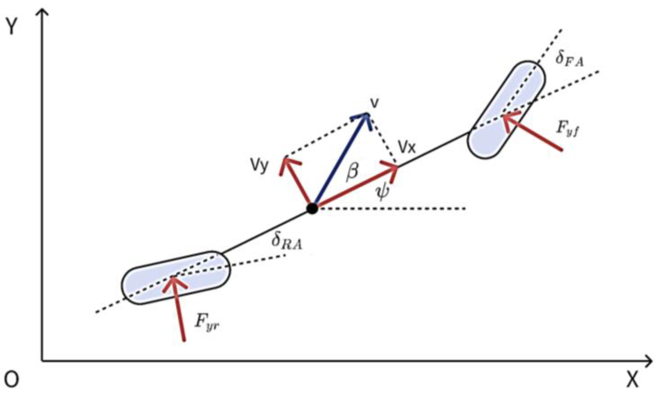
The two-degrees-of-freedom vehicle kinematic model simplifies vehicle motion to the absolute velocity and the yaw angle , without considering forces like tire dynamics or suspension [11]. To describe the general motion of a rigid body, Figure 1 gives the ISO convention plane and the vehicle state equipped with Four-Wheel Steer.
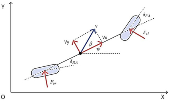
Figure 1.
The ISO convention plane and the vehicle state which equipped with Four-Wheel Steer.
For the translational motion component of the vehicle, we can directly derive the following equation:
In which and are the velocity and sideslip angle of the vehicle, and and are the longitudinal and lateral acceleration, respectively.
For the rotation motion component of the vehicle, we can obtain the following equation based on the theorem of rigid body rotational motion:
In which are the yaw angle and the absolute acceleration of the vehicle. And the acceleration can be described as follows:
Combined with Equations (2) and (3), it leads to the following:
Consequently, the 2-DOF kinematic model can be written into a standard state space form as follows:
Based on this kinematic model, we only need longitudinal acceleration, lateral acceleration, and yaw rate to estimate the two state variables theoretically. The above signals can be obtained from the IMU, but the noise and drift are inevitable. And these signal characteristics lead to significant errors in state estimates over time if there is no additional feedback observation.
2.2. The Bicycle Dynamic Model
In the field of vehicle control, there are various dynamic modeling approaches, including 7 degrees of freedom, 13 degrees of freedom, and others. However, for estimating the vehicle sideslip angle, the bicycle model is commonly used. This model is simple in structure and adequately supports sideslip angle estimation, which is shown in Figure 1. By using Newton’s law of motion, the lateral dynamics of the bicycle model are described as follows.
In which is the vehicle mass, is the equivalent yaw moment of inertia, and are the lateral tire force of front and rear wheel, respectively, and are the steer angle of front wheel and rear wheel, and and are the distance from the vehicle center of gravity to front and rear axles.
The lateral force in Equation (6) is calculated by calibrated magic tire model, as shown in Equation (7):
In which are the normalized stiffness coefficient of the linear region, is the maximum lateral adhesion coefficient, is the sideslip angle when reach the maximum lateral acceleration, and is the parameter to adjust the tire characteristic curve for large slip angles.
The parameter required in Equation (7) can be calibrated on the road with different friction coefficients. One thing to note is that, during real vehicle calibration, is typically less than 1, like the in Figure 2. This means that, with high slip rates, the vehicle’s achievable lateral capability will decrease. However, while such a tire curve can more accurately describe the tire’s dynamic behavior, it will cause the estimation results to incorrectly predict larger sideslip angle when beyond the maximum adhesion limit and fail to converge. Therefore, a value slightly greater than one is applied in this paper to make the tire characteristic curve is monotonically increasing.
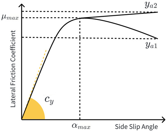
Figure 2.
The adjustment the tire model parameter .
3. UKF-Based Estimation Method
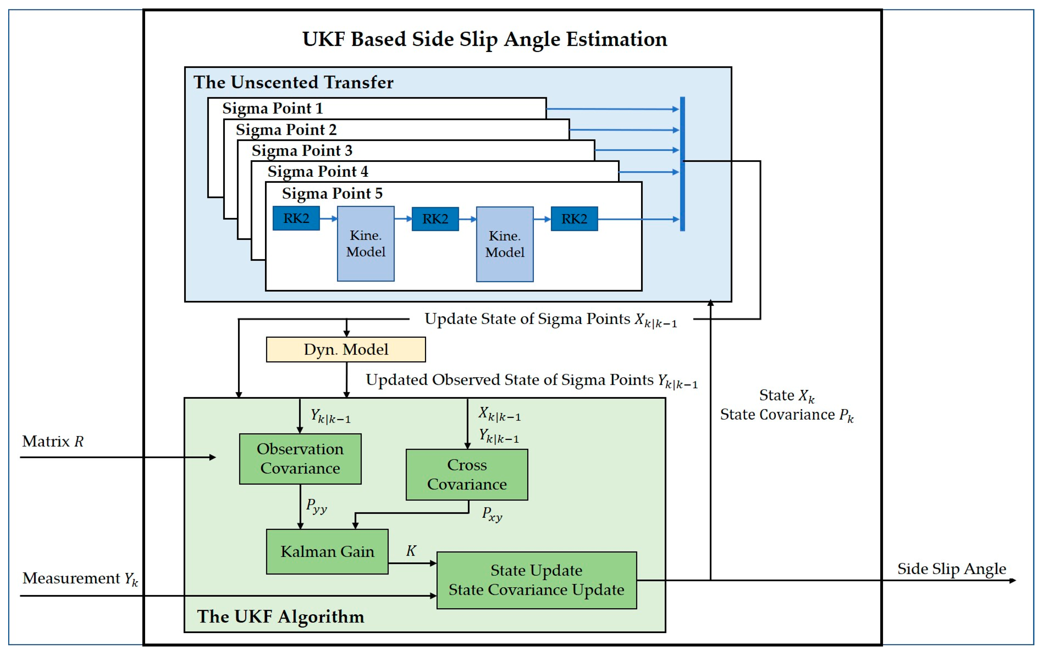
The UKF uses a deterministic sampling technique called Unscented Transform to better capture and propagate uncertainty through nonlinear transformations. The structure of the UKF-based sideslip angle estimation is given in Figure 3, and detailed calculation process is summarized in Algorithm 1. In general, this architecture employs vehicle kinematics model to update the state of each sigma point, which includes the velocity and sideslip angle of the vehicle. Then, the vehicle dynamic model is adopted to transfer the state sigma points to measurement space, which includes the lateral acceleration and the derivative of the yaw rate. Finally, the lateral acceleration and the derivative of the yaw rate obtained from the IMU measurements are used for state observation and update.
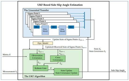
Figure 3.
The total structure of the UKF-based sideslip angle estimation.
The unscented transfer includes three steps (Steps 1–3 in Table 1):

Table 1.
The introduction of drive scenario.
Select a set of points based on input disturbance.
In which is the number of dimensions and is a tuning parameter and usually makes . is the covariance matrix of prior estimate and is the prior estimated state. is the column of the matrix square root of .
Propagate each selected point through the vehicle kinematic model.
The vehicle kinematic model formulated by Equation (5) is applied to propagate the selected points and produce a new set of points . To improve the approximation of solutions to the vehicle kinematic model, the second-order Runge–Kutta (RK2)filter is applied in this step.
Compute sigma points weight and approximate the mean and covariance of the propagated state.
The weight of sigma points is calculated as follows:
where is the weight of first propagated sigma point and is the weight of propagated sigma point .
Then, the mean of propagated state is as follows:
And the covariance of the propagated state is as follows:
In which is the covariance matrix that describes the process state uncertainty.
Before applying UKF algorithm to achieve state update, the vehicle dynamic model is adopted to transfer the state sigma points to measurement space .
Thence, the mean of measurement vector is as follows:
The covariance matrix of the measurement and the cross-covariance of the state and the measurement is as follows:
where is the covariance matrix that describes the squared measurement uncertainty.
The Kalman gain is given by the following:
Finally, the state and the covariance matrix of current state estimation is updated by the following:
In which is the measured lateral acceleration and the derivative of the yaw rate.
| Algorithm 1. UKF-based sideslip angle estimation |
| and last state |
is the |
| Step 3: Calculate the |
is the |
| Step 5: Calculate the and covariance matrix of the measurement |
| Step 6: Calculate the cross-covariance of the state and the measurement and the Kalman gain |
| Step 7: Update the |
4. Adaptive UKF Strategy
Many studies use fixed parameters to design unscented Kalman filters, assuming that the confidence in the system model and measurements remains constant. However, this assumption does not always align with real-world conditions. For example, as the tire slip angle increases, the accuracy of the vehicle dynamics model estimation significantly decreases. Using the same confidence coefficients in such cases can lead to biases in the estimation of the sideslip angle [6].
With this as motivation, this chapter will delve into analyzing the confidence levels of the system model and measurements under different conditions. This will be reflected through a covariance matrix of measurement uncertainty and state uncertainty in the UKF, leading to the design of the adaptive strategy. Furthermore, considering the significant impact of the state uncertainty on the entire system, as indicated in Equations (11) and (16), an excessively large will cause to increase significantly. This leads to an overly dispersed selection of Sigma points in the UKF, which reduces the accuracy of these sigma points in approximating the current conditions. Therefore, for this study, we decided to use a fixed Q matrix and a variable R matrix.
According to the author’s understanding, the following factors can affect the estimation of the sideslip angle: vehicle reference speed, road surface friction coefficient, and steering characteristics.
- Vehicle reference speed: This is one of the most important parameters of vehicle dynamic control. In the application of sideslip angle estimation, it is challenging to accurately calculate the tire sideslip angle at low speed, since the reference speed is in the numerator. This characteristic affects both the kinematic vehicle model and dynamic vehicle model. However, considering that the kinematics involves open-loop integration, the impact is somewhat greater. Therefore, it is preferable to rely more on the vehicle dynamic model for the estimation of the vehicle state with the decrease in speed.
- Surface friction coefficient: During low-traction driving conditions, such as navigating icy or snowy loops, tires can remain in the nonlinear region for extended periods. Relying solely on kinematic models in these situations can lead to non-convergent estimates. To address this challenge, there should be a greater emphasis on dynamic models. However, when making rapid turns on low-traction surfaces, the sideslip angle can quickly increase and maintain a relatively high value. According to the model adjustments in Figure 2, dynamic models cannot achieve accurate estimates under large sideslip angle conditions. Therefore, kinematic estimation needs to be promptly integrated and should play a leading role in the estimation process.
On high-traction surfaces, during aggressive steering maneuvers, vehicle states such as lateral angular velocity and yaw acceleration can change dramatically. In such scenarios, kinematic estimation is necessary to some extent to enhance the response speed of the estimation.
The accuracy of dynamic estimation heavily relies on the friction coefficient. Consequently, if there is insufficient confidence in the estimated value of adhesion, the accuracy of dynamic estimation may be compromised.
- Lateral characteristics: When turning rapidly, the use of kinematics should be increased, as discussed in the section of surface friction coefficient. Quickly turning the steering wheel can also lead to significant under-steering, especially on low-traction surfaces. Significant oversteering means the wheels have entered the nonlinear zone. Due to adjustments made to the nonlinear zone of the tire model, as shown in Figure 2, errors can easily occur in the estimation of the sideslip angle based on wheel dynamics in this situation.
Hence, the adaptive strategy can be summarized as follows, and the measurement uncertainty is formulated as Equation (18). It should be noted that smaller means allocating more weightiness to dynamic estimation.
- ➢
- : Slightly decrease the covariance matrix of measurement uncertainty with the decrease in reference speed;
- ➢
- : In low-traction situations, the baseline value of the measurement uncertainty should be significantly smaller, which means that dynamic estimation plays a leading role.
- ➢
- When detecting rapid steering (with large steer wheel angle speed) by the driver, measurement uncertainty needs to be increased quickly, and its upper limit should be more flexible than that in high-traction conditions, as shown in Figure 4.
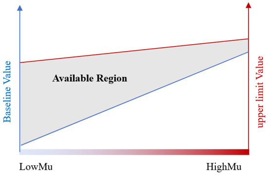 Figure 4. The schematic diagram of adaptive coefficient changes on different adhered surfaces.
 - ➢
- When there is a significant jump in the estimated value of the friction coefficient, it is appropriate to increase the measurement uncertainty .
- ➢
- When understeer or oversteer condition is detected, increase the measurement uncertainty . The coefficient of understeer or oversteer is calculated by the relationship between yaw rate, lateral acceleration, and steer wheel angle.
The parameters of all functions in Equation (18) are calibrated based on real vehicle tests, with the test conditions covering various adhesion levels and driving intensities.
5. Experiment Verification
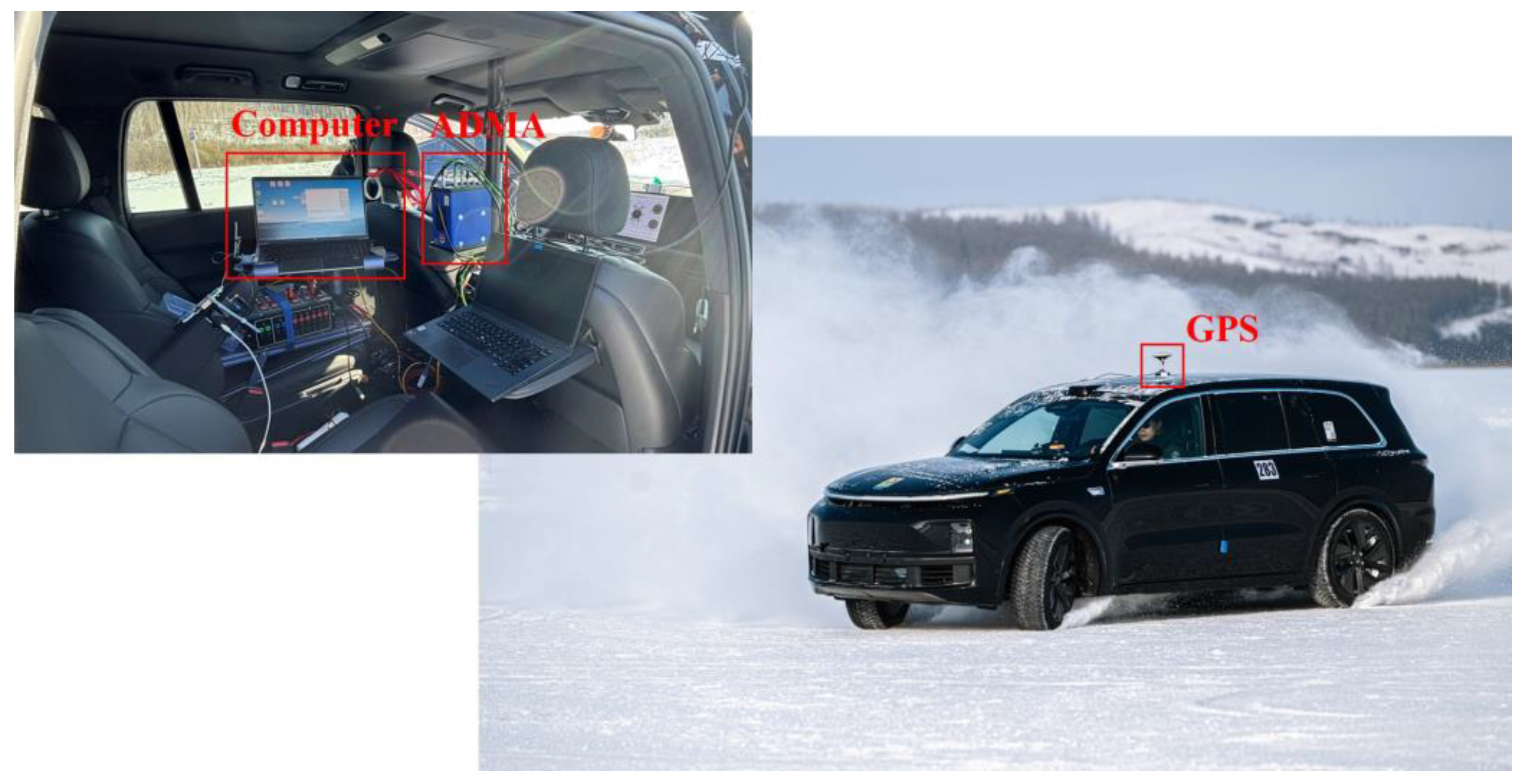
In this section, the proposed estimation algorithm is evaluated with real experimental tests. As Shown in Figure 5, the Four-Wheel Steer Li-Auto is equipped with the Automotive Dynamic Motion Analyzer (ADMA), which is integrated with Differential Global Navigation Satellite System (DGNSS) and fiber optic gyroscopes to measure the acceleration, speed, and position of moving vehicles in all three dimensional axes constantly. The control algorithm is compiled and programmed into a production controller, and vehicle signals are acquired through CAN communication. The scenarios for the test dataset to verify the performance of the algorithm are listed in Table 1.
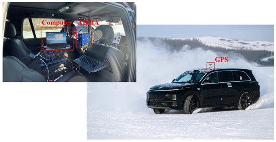
Figure 5.
The test vehicle: Li-Auto equipped with ADMA.
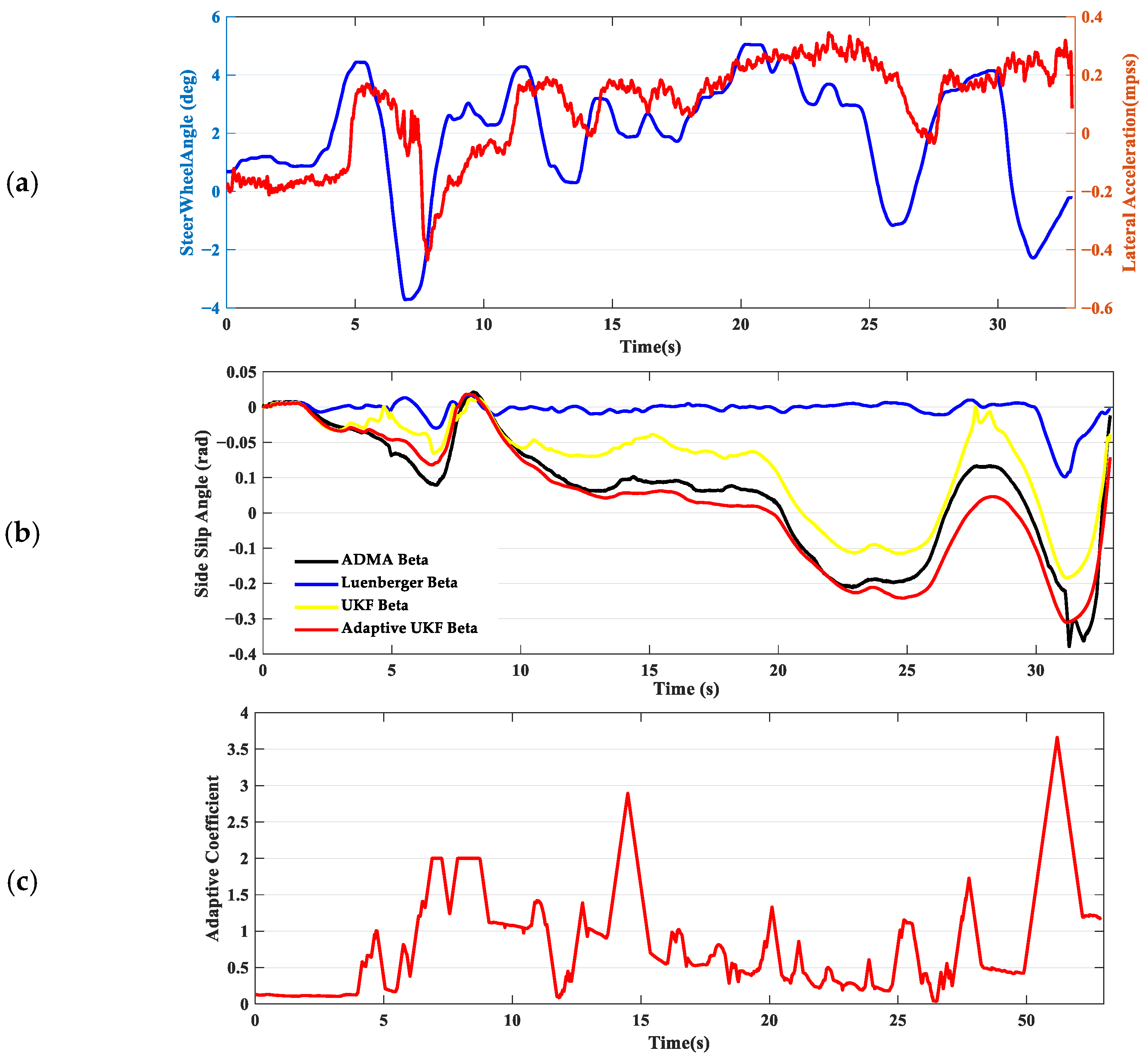
In scenario 1, the driver controls the steer wheel, acceleration pedal, and brake pedal to make the vehicle maintain a steady circular motion on the ice ring, and the reference speed is about 40 kph. The steer angle is given in Figure 6a, along with the lateral acceleration. In this scenario, the vehicle maintains a large slip angle for an extended period, and the tires are constantly in a nonlinear region. From the real vehicle test data, the estimation strategy based on the Luenberger observer performs poorly under these operating conditions, showing significant estimation errors, and the max error reaches 0.291 rad. Otherwise, the estimated values still demonstrate good convergence characteristics. The UKF increases the adaptive coefficients (the R matrix) when the tires experience sustained large slip. This adjustment reduces the reliance on the dynamic model. The data results confirm that this adaptive logic can effectively improve the estimation accuracy of the slip angle. As shown in Figure 6b, the estimation error is appropriately reduced after adopting the adaptive strategy, and the Root Mean Square Error (RMSE) decreases from 0.0436 rad to 0.0386 rad, as shown in Table 2.
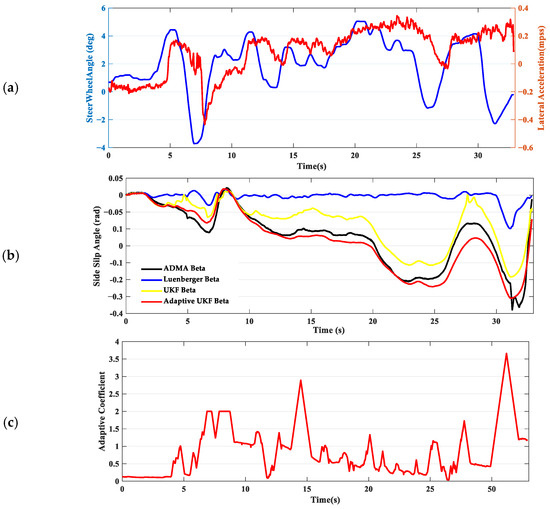
Figure 6.
The test data of scenario 1: cycle drive on ice road. (a) Steer wheel angle and lateral acceleration. (b) The estimation sideslip angle. (c) Adaptive coefficient.
Table 2.
Root Mean Square Error (RMSE) and max error of different scenarios.
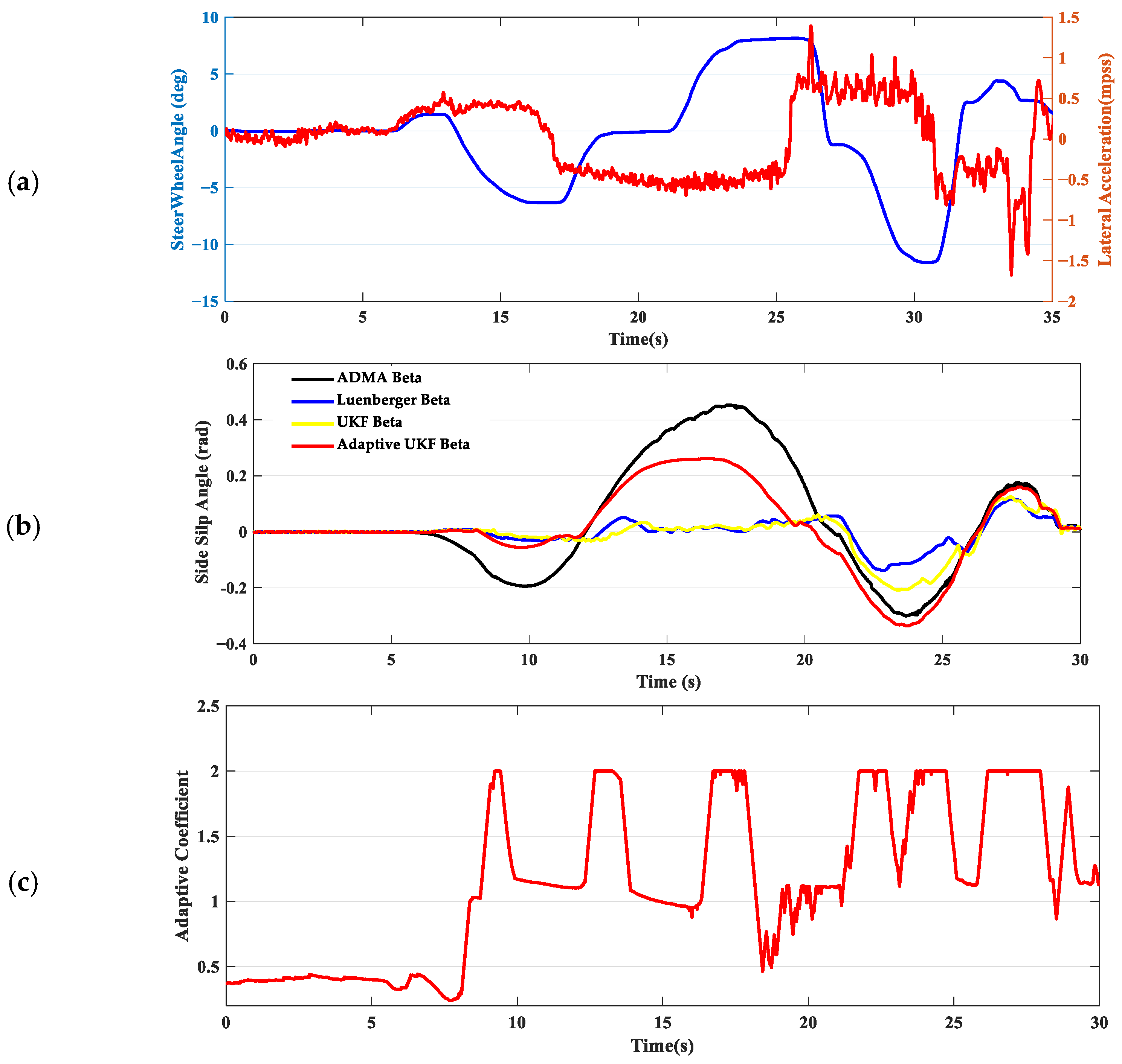
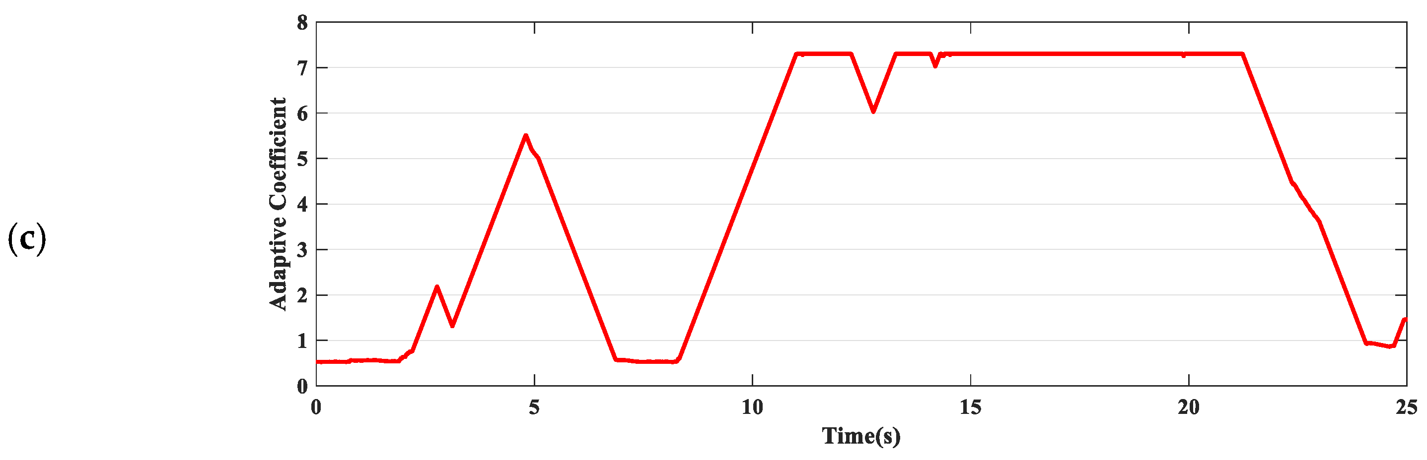
In scenario 2, the driver performs a double lane change maneuver on an icy surface. In this situation, the vehicle is prone to experiencing understeer. As shown in Figure 7c, the adaptive strategy maintains the adaptive coefficients at a high level when detecting vehicle understeer. If the driver turns the steering wheel quickly beyond the road’s adhesion capability, the strategy further increases the adaptive coefficients. With this feature, the estimation of the sideslip angle is significantly improved, and the estimation accuracy is noticeably better than the other two sets of results (the RMSE is approximately half of that of the other two estimation strategies). More specifically, around 12 s, only the adaptive UKF brings the estimated value of the sideslip angle close to the true value. This is also due to the adaptive strategy providing a large R at that time.
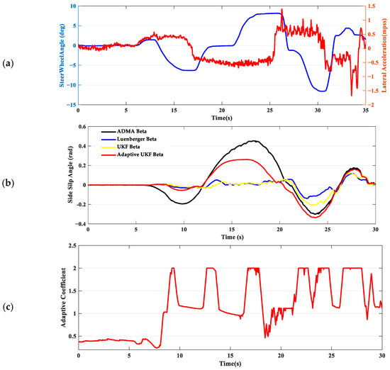
Figure 7.
The test data of scenario 2: double lane change on ice road. (a) Steer wheel angle and lateral acceleration. (b) The estimation sideslip angle. (c) Adaptive coefficient.
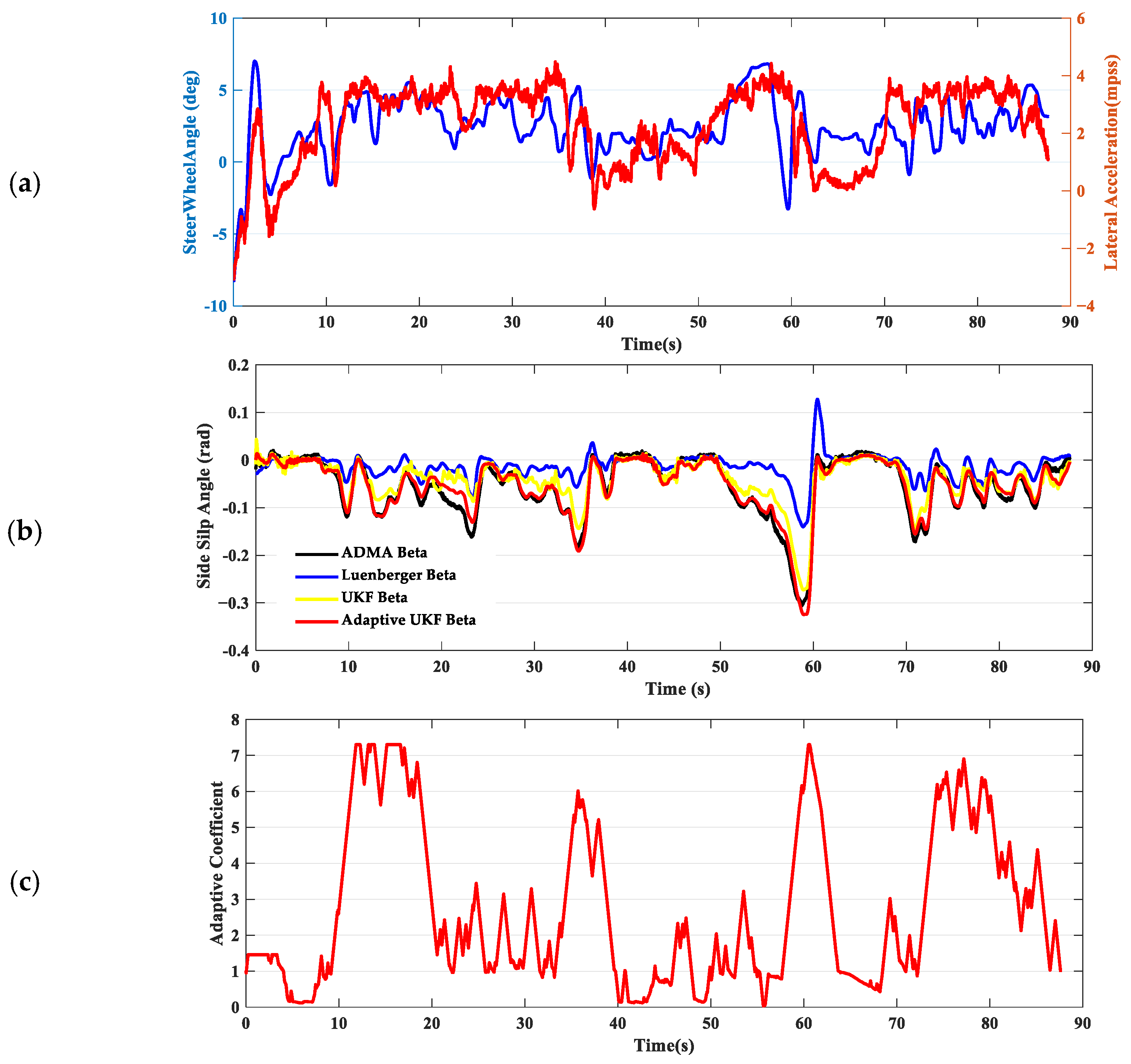
In scenario 3, the driver controls the vehicle maintain a steady circular motion on the snow ring, and the reference speed is about 60 kph. The test results similarly indicate that the adaptive strategy achieves good estimation accuracy, consistent with the findings from the ice circle tests. It is noteworthy that, around 50–60 s, the driver executed an aggressive maneuver to induce oversteer and rapid steering/throttle control to restore the vehicle’s stability. During this process, the adaptive UKF demonstrated better estimation accuracy compared to the Luenberger observer. This effectively proves that the adaptive UKF has significant advantages under extreme conditions, in which the tires operate in nonlinear regions.
In scenario 4, the driver performed a double lane change maneuver on a snow surface. The traction coefficient on snow is approximately 0.4, which means the adaptive coefficients would also be somewhat larger compared to those on ice, as shown in Figure 8c. However, when there is no strategy for adaptively adjusting the weights based on the traction coefficient, the UKF’s estimation results on snow are not very ideal, as shown in Figure 9b. In some extreme situations, such as around 10 s and 17 s, the estimation accuracy is slightly inferior due to not utilizing the kinematic estimation results more effectively.
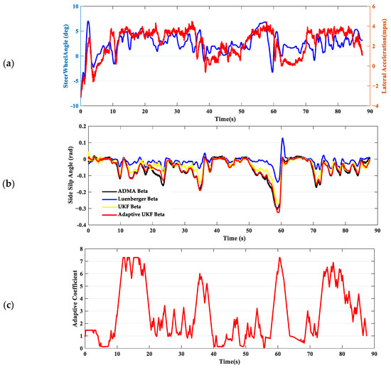
Figure 8.
The test data of scenario 3: cycle drive on snow road. (a) Steer wheel angle and lateral acceleration. (b) The estimation sideslip angle. (c) Adaptive coefficient.
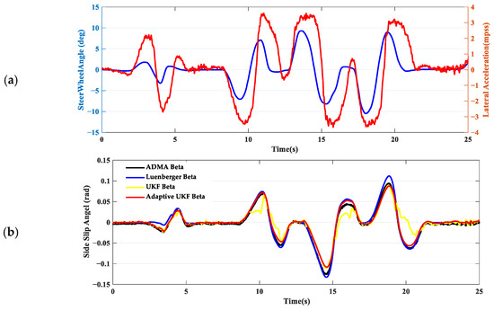
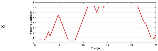
Figure 9.
The test data of scenario 4: lane change on snow road. (a) Steer wheel angle and lateral acceleration. (b) The estimation sideslip angle. (c) Adaptive coefficient.
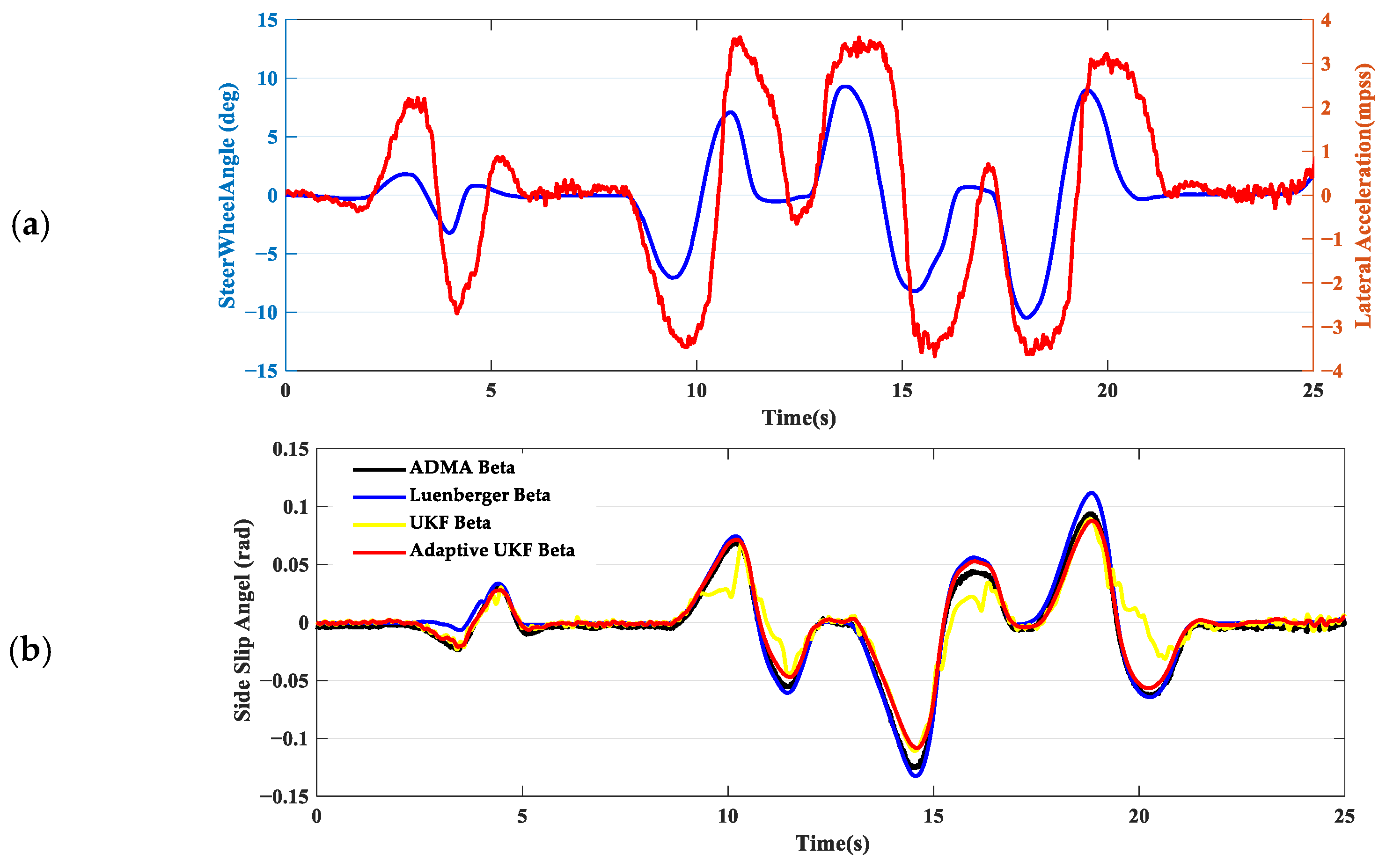
In scenario 5, the driver performs a relatively smooth slalom maneuver on an asphalt surface, maintaining a speed around 80 kph, with lateral acceleration approximately between 0.2 and 0.3 g. From the comparison of the maximum estimation error and the deviation in RMSE presented in Table 2, there is not a significant difference among the three estimates. The biggest difference is that the UKF estimation results without an adaptive strategy are relatively rough. This is mainly because a fixed smaller R is used to ensure system convergence, leading to a significantly increased feedback gain based on model errors. As a result, this can cause overshoot in the estimation, which in turn makes the estimation of the sideslip angle exhibit spikes. In comparison with the adaptive coefficient under low adhesion conditions, the adaptive coefficient of the system on asphalt surfaces is significantly larger, as shown in Figure 10c. The results not only ensure estimation accuracy, but also provide smoother estimates, which effectively verifies the correctness of increasing the adaptive coefficient as the friction coefficient increases.
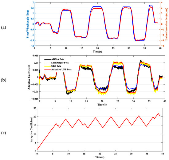
Figure 10.
The test data of scenario 5: slalom on asphalt road. (a) Steer wheel angle and lateral acceleration. (b) The estimation sideslip angle. (c) Adaptive coefficient.
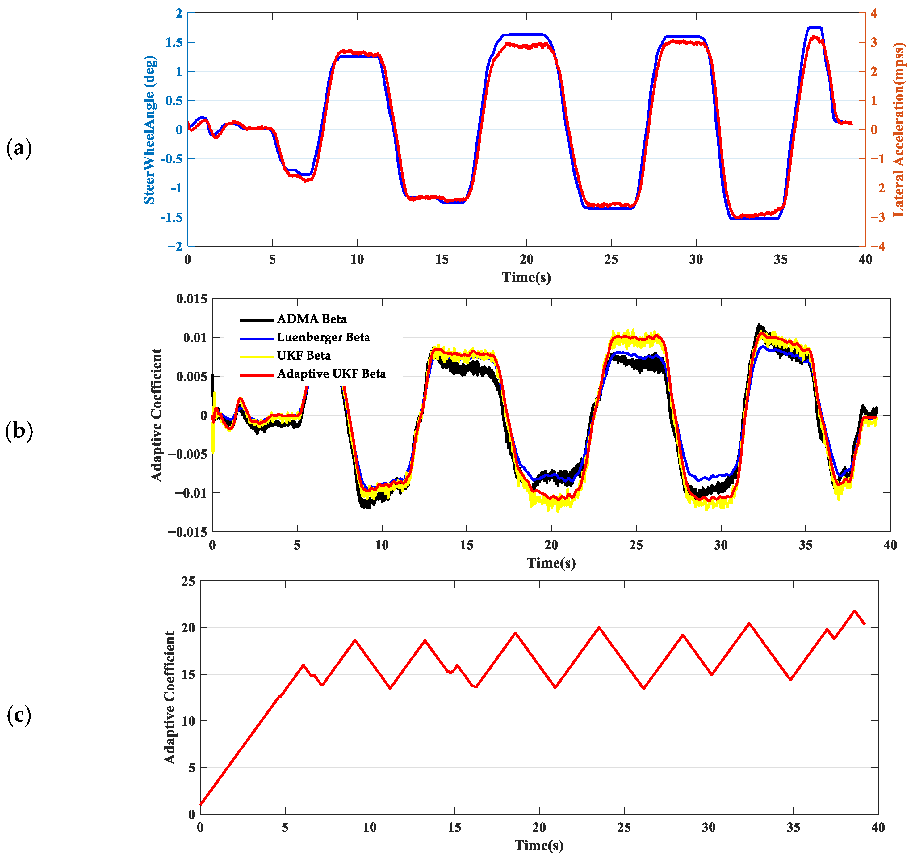
In scenario 6, the driver performs a sharply double lane change on an asphalt surface, accelerating speed from 40 to 90 kph, with lateral acceleration approximately between 0.7 and 0.8 g. As vehicle speed increases, the adaptive coefficient also tends to increase. From the test results, the adaptive UKF strategy is more capable of sensitively and quickly capturing the short-term sideslip angle reversal effect caused by the phase difference between lateral acceleration and yaw when the driver turns the steering wheel. Comparing the test results given in Figure 11, we can conclude that the estimation accuracy of the adaptive UKF strategy is slightly better than that of the Luenberger observer and also smoother than the standard UKF estimation results.
Figure 11.
The test data of scenario 6: lane change on asphalt road. (a) Steer wheel angle and lateral acceleration. (b) The estimation sideslip angle. (c) Adaptive coefficient.
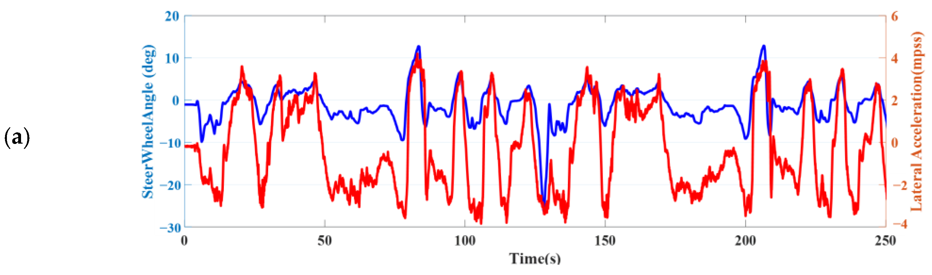
In scenario 7, the driver drives in handling course covered by snow, with parts where the underlying ice of the lake is exposed due to repeated tire friction. Based on the statistical data, the UKF demonstrates higher estimation accuracy under these complex driving conditions. Compared to the Luenberger observer, the root mean square of the estimation error is reduced by 47%. In terms of details, Figure 12 presents two subplots. In Subplot 1, the driver navigates the curve using a drifting technique. By continuously adjusting the steering angle, the vehicle maintains a relatively stable sideslip angle and lateral acceleration while cornering. The adaptive UKF can accurately estimate the sideslip angle immediately when the steering wheel is turned, benefiting from the increased R. In comparison, the UKF gradually approaches the correct sideslip angle estimation as further steering adjustments are made. Under these aggressive driving conditions, the Luenberger observer consistently exhibits significant deviations in its estimates. In Subplot 2, the vehicle experiences oversteer, and throughout this process, the adaptive UKF maintains the best estimation accuracy.

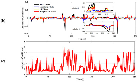
Figure 12.
The test data of scenario 7: handling course drive. (a) Steer wheel angle and lateral acceleration. (b) The estimation sideslip angle. (c) Adaptive coefficient.
6. Conclusions
This research seeks to harness the full potential of the Unscented Kalman Filter (UKF) for nonlinear estimation, developing adaptive strategies to accurately estimate the sideslip angle across diverse conditions and scenarios. The proposed sideslip angle estimation framework employs a linear two-degree-of-freedom vehicle kinematic model for iterative state updates and a vehicle dynamics model for state observation. By integrating theoretical insights with real-world testing experience, this study analyzes and compares the performance and applicability of kinematic and dynamic models under various conditions, summarizing patterns based on adhesion friction, speed, and lateral characteristics. Ultimately, it proposes an adaptive strategy for the covariance matrix of measurement uncertainty to optimize the contribution of both models to the final estimation in complex scenarios.
The adaptive UKF-based sideslip angle estimation strategy is validated using real vehicle tests and compared against the Luenberger observer and a well-tuned UKF observer. The results demonstrate that the adaptive UKF strategy significantly improves slip angle estimation accuracy in low-friction scenarios (such as on ice and snow), especially under conditions where aggressive driving pushes tires into nonlinear operational regions (including oversteering and understeering). For example, the maximum estimation error decreased by 91.37% and 77.18% compared to the Luenberger observer and a well-tuned UKF observer in scenario 1, respectively. Additionally, the adaptive strategy effectively addresses the challenge of balancing estimation accuracy and smoothness in varying friction conditions, achieving excellent performance in both smoother operations and more aggressive maneuvers on high-friction surfaces.
Author Contributions
Conceptualization, L.Z. and J.W.; methodology, J.W. and Y.H.; software, J.W. and Y.H.; validation, J.W. and Y.H.; formal analysis, J.W.; investigation, Y.H.; resources, L.Z. and L.L.; data curation, curation, L.Z. and J.W.; writing—original draft preparation, curation, J.W.; writing—review and editing, L.Z. and L.L.; visualization, J.W.; supervision, L.Z. and L.L.; project administration, L.Z. and L.L. All authors have read and agreed to the published version of the manuscript.
Funding
This research received no external funding.
Data Availability Statement
The data that support the findings of this study are available from the corresponding authors upon reasonable request.
Conflicts of Interest
The authors Liang Zhao, Jiawei Wang and Yingjia Hu were employed by the company Shanghai Lixiang Technology Co., Ltd. The remaining authors declare that the research was conducted in the absence of any commercial or financial relationships that could be construed as a potential conflict of interest.
References
- Piyabongkarn, D.; Rajamani, R.; Grogg, J.A.; Lew, J.Y. Development and Experimental Evaluation of a Slip Angle Estimator for Vehicle Stability Control. IEEE Trans. Control Syst. Technol. 2009, 17, 78–88. [Google Scholar] [CrossRef]
- Jeong, D.; Ko, G.; Choi, S.B. Estimation of sideslip angle and cornering stiffness of an articulated vehicle using a constrained lateral dynamics model. Mechatronics 2022, 85, 102810. [Google Scholar] [CrossRef]
- Biase, F.D.; Lenzo, B.; Timpone, F. Vehicle Sideslip Angle Estimation for a Heavy-Duty Vehicle via Extended Kalman Filter Using a Rational Tyre Model. IEEE Access 2020, 8, 142120–142130. [Google Scholar] [CrossRef]
- Zhang, C.; Feng, Y.; Wang, J.; Gao, P.; Qin, P. Vehicle Sideslip Angle Estimation Based on Radial Basis Neural Network and Unscented Kalman Filter Algorithm. Actuators 2023, 12, 371. [Google Scholar] [CrossRef]
- Tufano, F.; Lui, D.G.; Battistini, S.; Lenzo, B.; Santini, S. Vehicle Sideslip Angle estimation under critical road conditions via nonlinear Kalman filter-based state-dependent Interacting Multiple Model approach. Control Eng. Pract. 2024, 146, 105901. [Google Scholar] [CrossRef]
- Battistini, S.; Brancati, R.; Lui, D.G.; Tufano, F. Enhancing ADS and ADAS Under Critical Road Conditions Through Vehicle Sideslip Angle Estimation via Unscented Kalman Filter-Based Interacting Multiple Model Approach. Mech. Mach. Sci. 2022, 122, 450–460. [Google Scholar]
- Gao, L.; Wu, Q.; He, Y.; Wu, K.; Shao, P. Robust Estimation of Sideslip Angle for Heavy-Duty Vehicles Under Payload Conditions Using a Series-Connected Structure Estimator; IEEE: New York, NY, USA, 2024. [Google Scholar]
- Napolitano Dell’Annunziata, G.; Ruffini, M.; Stefanelli, R.; Adiletta, G.; Fichera, G.; Timpone, F. Four-Wheeled Vehicle Sideslip Angle Estimation: A Machine Learning-Based Technique for Real-Time Virtual Sensor Development. Appl. Sci. 2024, 14, 1036. [Google Scholar] [CrossRef]
- Kim, D.; Kim, G.; Choi, S.; Huh, K. An Integrated Deep Ensemble-Unscented Kalman Filter for Sideslip Angle Estimation with Sensor Filtering Network. IEEE Acces 2021, 9, 149681–149689. [Google Scholar] [CrossRef]
- Bonfitto, A.; Feraco, S.; Tonoli, A.; Amati, N. Combined regression and classification artificial neural networks for sideslip angle estimation and road condition identification. Veh. Syst. Dyn. 2019, 58, 1766–1787. [Google Scholar] [CrossRef]
- Bertipaglia, A.; Alirezaei, M.; Happee, R.; Shyrokau, B. An Unscented Kalman Filter-Informed Neural Network for Vehicle Sideslip Angle Estimation. IEEE Trans. Veh. Technol. 2024, 73, 12731–12746. [Google Scholar] [CrossRef]
- Park, G. Vehicle Sideslip Angle Estimation Based on Interacting Multiple Model Kalman Filter Using Low-Cost Sensor Fusion. IEEE Trans. Veh. Technol. 2022, 71, 6088–6099. [Google Scholar] [CrossRef]
- Liu, W.; Xiong, L.; Xia, X.; Lu, Y.; Gao, L.; Song, S. Vision-aided Intelligent Vehicle Sideslip Angle Estimation Based on Dynamic Model. IET Intelligent Transport Systems 2020, 14, 1183–1189. [Google Scholar] [CrossRef]
- Serena, L.; Bruschetta, M.; de Castro, R.; Lenzo, B. Estimating Sideslip Angle Using a Downward-Facing Camera. Paper presented at Italian Mechanism Science. IFToMM Italy 2024. Mech. Mach. Sci. 2024, 164, 290–297. [Google Scholar]
- Xia, X.; Hashemi, E.; Xiong, L.; Khajepour, A. Autonomous Vehicle Kinematics and Dynamics Synthesis for Sideslip Angle Estimation Based on Consensus Kalman Filter. IEEE Trans. Control Syst. Technol. 2023, 31, 179–192. [Google Scholar] [CrossRef]
- Novi, T.; Capitani, R.; and Annicchiarico, C. An integrated artificial neural network–unscented Kalman filter vehicle sideslip angle estimation based on inertial measurement unit measurements. Proc. Inst. Mech. Eng. Part D J. Automob. Eng. 2018, 233, 1864–1878. [Google Scholar] [CrossRef]
- Li, J.; Feng, B.; Zhang, L.; Luo, J. Research on Vehicle Stability Control Based on a Union Disturbance Observer and Improved Adaptive Unscented Kalman Filter. Electronics 2024, 13, 3220. [Google Scholar] [CrossRef]
- Viadero-Monasterio, F.; García, J.; Meléndez-Useros, M.; Jiménez-Salas, M.; Boada, B.L.; López Boada, M.J. Simultaneous Estimation of Vehicle Sideslip and Roll Angles Using an Event-Triggered-Based IoT Architecture. Machines 2024, 12, 53. [Google Scholar] [CrossRef]
- Boada, B.L.; Viadero-Monasterio, F.; Zhang, H.; Boada, M.J.L. Simultaneous Estimation of Vehicle Sideslip and Roll Angles Using an Integral-Based Event-Triggered H∞ Observer Considering Intravehicle Communications. IEEE Trans. Veh. Technol. 2023, 72, 4411–4425. [Google Scholar] [CrossRef]
- Righetti, G.; Lenzo, B. A Combined Dynamic–Kinematic Extended Kalman Filter for Estimating Vehicle Sideslip Angle. Appl. Sci. 2025, 15, 1365. [Google Scholar] [CrossRef]
- Chen, B.C.; Hsieh, F.C. Sideslip angle estimation using extended Kalman filter. Veh. Syst. Dyn. 2008, 46, 353–364. [Google Scholar] [CrossRef]
- Sun, W.; Wang, Z.; Wang, J.; Wang, X.; Liu, L. Research on a Real-Time Estimation Method of Vehicle Sideslip Angle Based on EKF. Sensors 2022, 22, 3386. [Google Scholar] [CrossRef] [PubMed]
- Villano, E.; Lenzo, B.; Sakhnevych, A. Cross-combined UKF for vehicle sideslip angle estimation with a modified Dugoff tire model: Design and experimental results. Meccanica 2021, 56, 2653–2668. [Google Scholar] [CrossRef]
- Li, G.; Zhao, D.; Xie, R.; Han, H.; Zong, C. Vehicle State Estimation Based on Improved Sage–Husa Adaptive Extended Kalman Filtering. Automot. Eng. 2015, 37, 1426–1432. [Google Scholar]
- Boada, B.L.; Boada, M.J.L.; Diaz, V. Vehicle sideslip angle measurement based on sensor data fusion using an integrated ANFIS and an Unscented Kalman Filter algorithm. Mech. Syst. Signal Process. 2016, 72, 832–845. [Google Scholar] [CrossRef]
- Xue, Z.; Cheng, S.; Li, L.; Zhong, Z.; Mu, H. A Robust Unscented M-Estimation-Based Filter for Vehicle State Estimation with Unknown Input. IEEE Trans. Veh. Technol. 2022, 71, 6119–6130. [Google Scholar] [CrossRef]
- Wang, Y.; Yan, Y.; Shen, T.; Bai, S.; Hu, J.; Xu, L.; Yin, G. An event-triggered scheme for state estimation of preceding vehicles under connected vehicle environment. IEEE Trans. Intell. Veh. 2022, 8, 583–593. [Google Scholar] [CrossRef]
- Wang, Y.; Li, Y.; Zhao, Z. State Parameter Estimation of Intelligent Vehicles Based on an Adaptive Unscented Kalman Filter. Electronics. 2023, 12, 1500. [Google Scholar] [CrossRef]
- Zhang, Y.; Li, M.; Zhang, Y.; Hu, Z.; Sun, Q.; Lu, B. An Enhanced Adaptive Unscented Kalman Filter for Vehicle State Estimation. IEEE Trans. Instrum. Meas. 2022, 71, 6502412. [Google Scholar] [CrossRef]
- Chen, Y.; Yan, H.; Li, Y. Vehicle State Estimation Based on Sage–Husa Adaptive Unscented Kalman Filtering. World Electr. Veh. J. 2023, 14, 167. [Google Scholar] [CrossRef]
- Alshawi, A.; De Pinto, S.; Stano, P.; van Aalst, S.; Praet, K.; Boulay, E.; Ivone, D.; Gruber, P.; Sorniotti, A. An Adaptive Unscented Kalman Filter for the Estimation of the Vehicle Velocity Components, Slip Angles, and Slip Ratios in Extreme Driving Manoeuvres. Sensors 2024, 24, 436. [Google Scholar] [CrossRef]
- Pang, H.; Wang, P.; Wang, M.; Hu, C. On accurate estimation of vehicle lateral states based on an improved adaptive unscented Kalman filter. Proc. Inst. Mech. Eng. Part D J. Automob. Eng. 2022, 238, 867–882. [Google Scholar] [CrossRef]


Disclaimer/Publisher’s Note: The statements, opinions and data contained in all publications are solely those of the individual author(s) and contributor(s) and not of MDPI and/or the editor(s). MDPI and/or the editor(s) disclaim responsibility for any injury to people or property resulting from any ideas, methods, instructions or products referred to in the content. |
© 2025 by the authors. Licensee MDPI, Basel, Switzerland. This article is an open access article distributed under the terms and conditions of the Creative Commons Attribution (CC BY) license (https://creativecommons.org/licenses/by/4.0/).