Text-Conditioned Diffusion-Based Synthetic Data Generation for Turbine Engine Sensor Analysis and RUL Estimation

Abstract

This paper introduces a novel framework for generating synthetic time-series data from turbine engine sensor readings using a text-conditioned diffusion model. The approach begins with dataset preprocessing, including correlation analysis, feature selection, and normalization. Principal Component Analysis (PCA) transforms the normalized signals into three components, mapped to the RGB channels of an image. These components, combined with engine identifiers and cycle information, form compact 19 × 19 × 3 pixel images, later scaled to 512 × 512 × 3 pixels. A variational autoencoder (VAE)-based diffusion model, fine-tuned on these images, leverages text prompts describing engine characteristics to generate high-quality synthetic samples. A reverse transformation pipeline reconstructs synthetic images back into time-series signals, preserving the original engine-specific attributes while removing padding artifacts. The quality of the synthetic data is assessed by training Remaining Useful Life (RUL) estimation models and comparing performance across original, synthetic, and combined datasets. Results demonstrate that synthetic data can be beneficial for model training, particularly in the early epochs when working with limited datasets. Compared to existing approaches, which rely on generative adversarial networks (GANs) or deterministic transformations, the proposed framework offers enhanced data fidelity and adaptability. This study highlights the potential of text-conditioned diffusion models for augmenting time-series datasets in industrial Prognostics and Health Management (PHM) applications.

1. Introduction

In the era of Industry 4.0, particularly in predictive maintenance, artificial intelligence (AI) has become increasingly significant. This growing interest has led to the extensive collection of industrial data through sensors that monitor variables such as electrical current, vibration, temperature, and pressure. These data are then leveraged to train models that analyze, diagnose, and predict the remaining useful life (RUL) and health indicators (HIs) of a system. The RUL represents the estimated time a component or system can continue operating before experiencing failure [1]. Similarly, the HI continuously monitors the condition of components, identifying significant changes that may indicate potential malfunctions or failures [1]. Rather than reacting to failures after they occur, these techniques allow for proactive failure prediction and prevention.

Predictive maintenance, also known as Prognostics and Health Management (PHM) [2], plays a critical role in industrial operations, directly influencing strategic decision making, maintenance scheduling, and failure prevention. This field is generally categorized into three main approaches: model-driven, data-driven, and hybrid models [3]. Model-driven approaches (also known as physics-driven) use mathematical models based on the physical behavior of components to develop predictive strategies [4]. Data-driven approaches analyze sensor data using machine learning (ML) and deep learning (DL) techniques to predict component degradation [3]. Hybrid models integrate both approaches, leveraging their strengths while mitigating individual limitations to achieve more accurate predictions [4].

Despite their advantages, physics-based and hybrid approaches face significant limitations, which have driven the growing adoption of data-driven models. In physics-based methods, one major challenge is the scarcity of physical degradation examples in complex systems. When such examples do exist, they typically pertain to highly specific components, limiting their applicability in systems with multiple components and failure modes [5]. Additionally, constructing a physics-based model can be extremely difficult, particularly in highly complex systems or under harsh operational conditions [3]. Similarly, while hybrid models attempt to mitigate these issues, they remain inadequate for systems where failure mechanisms cannot be explicitly modeled [1]. Due to these constraints, data-driven approaches have experienced rapid adoption in industrial applications, offering a more scalable and flexible alternative.

In data-driven approaches, the availability of data is a key factor, as these methods rely on publicly available datasets for training. Among these, C-MAPSS is the most widely used (23%), followed by FEMTO-ST PRONOSTIA (16%). The most common data sources in predictive maintenance include bearings (29%), dual-flow jet engines (21%), batteries (20%), and cutting tools (8%) [1,6].

When working with datasets, both the quality and quantity of available data are crucial factors in model training. However, acquiring sufficient high-quality data, especially in the context of PHM, remains a significant challenge and can lead to performance degradation. To address this issue, artificial intelligence offers an effective solution known as data augmentation, which enhances dataset diversity and improves model robustness. Data augmentation involves artificially generating new data from existing samples to enhance AI model training [7]. This technique not only improves model performance but also strengthens data privacy, reduces reliance on limited datasets, increases data diversity, balances class distributions, and mitigates the risk of overfitting.

In the context of predictive maintenance, several innovative approaches have explored the use of data augmentation to enhance model performance. For example, Wang et al. [3] introduced an autoregressive method that leverages historical component data to guide real-time data generation, enabling more accurate state predictions. Variational Autoencoders (VAEs) have also been employed for data augmentation, where an embedding vector is learned and passed to a decoder to synthesize new samples [8]. While VAEs are effective for learning compact latent representations, it is well-documented that they often struggle to generate high-quality samples, which can limit their effectiveness in scenarios requiring high fidelity and detail.

Rohan [4] combined signal processing techniques, transfer learning, and Generative Adversarial Networks (GANs) to synthesize failure data, achieving improved accuracy compared to traditional approaches. Cofré-Martel [5] proposed a methodology for generating features that evaluate health indicators (HIs), contributing to more effective condition monitoring of systems.

Zheng et al. [9] developed GAN-FAN, a novel architecture based on multiple GANs, designed specifically to address class imbalance by generating synthetic samples. Compared to methods such as InfoGAN and ADASYN, GAN-FAN showed significant improvements in the quality of generated data. However, GAN-based techniques often inherit and may even amplify biases present in the training data [10].

In response to these limitations, Solis-Martin et al. [11] proposed the use of Denoising Diffusion Probabilistic Models (DDPMs) for time-series data augmentation. Their approach conditions the generative process on a predefined set of meta-attributes, enabling the synthesis of realistic and diverse time-series samples for PHM applications. However, a notable limitation of this method is the requirement to predefine the set of meta-attributes relevant to the task, which may reduce flexibility and require domain-specific expertise for effective implementation.

While the aforementioned approaches have shown potential for enhancing PHM through data augmentation, most rely on generative models such as GANs [12] and VAEs, which often suffer from training instability or limited sample quality, respectively. Many works have focused on addressing the training instability of GAN models [13,14,15]; however, this remains one of the main challenges of these models. Models like VQ-VAEs have improved the quality of the samples generated by VAEs [16], thanks to a discrete representation of the inputs. However, VQ-VAEs are primarily focused on image processing and require further adaptation to be applied to signal processing. Newer generative frameworks, particularly Denoising Diffusion Probabilistic Models (DDPMs), offer significant advantages in terms of stability and output fidelity. However, their application in the PHM domain remains limited.

In contrast to the previously mentioned work by Solis-Martin et al. [11], the approach proposed in this study introduces a novel conditioning mechanism based on natural language prompts. This enables the generative model to produce data that are not only realistic but also semantically aligned with the intended context. To the best of our knowledge, this represents the first application of text-conditioned diffusion models for synthetic data generation in the PHM domain. By incorporating descriptive textual metadata during the generation process, our method ensures that the synthesized samples accurately reflect the desired operational states or failure modes, providing greater control and flexibility in data augmentation pipelines.

This study introduces a novel approach for enhancing predictive maintenance through the use of synthetic data generation via diffusion models. The key contributions of this work are summarized as follows:

• Synthetic Data Generation for PHM: This work explores the application of Denoising Diffusion Probabilistic Models (DDPMs) for generating high-quality synthetic datasets, addressing the challenges posed by limited real-world industrial data.
• Text-Conditioned Data Augmentation: The study introduces a text-conditioning mechanism that enhances the control and interpretability of the generated synthetic data, allowing the expansion of datasets beyond the original categories.
• Feature Selection and Data Preprocessing: A systematic feature selection process was conducted, removing redundant and non-informative attributes to improve the efficiency and accuracy of the Remaining Useful Life (RUL) prediction models.
• Image-Based Representation of Time-Series Data: An approach was implemented to transform time-series sensor data into an image representation, enabling the effective use of generative models while preserving critical structural and statistical properties.
• RUL estimation effectiveness: The proposed method has been demonstrated to be effective even with a very limited amount of data, which is particularly valuable in PHM applications where data scarcity is one of the main challenges.

The paper is structured as follows. Section 2 outlines the techniques and algorithms used in the study; Section 3 details the data selection process, preprocessing steps, data expansion, and the generation of synthetic data used in the experiments; Section 4 presents the experimental findings, assessing the performance of the trained models; Section 5 analyzes the implications of the results, highlighting potential limitations; and Section 6 summarizes the key insights and overall findings of the study.

2. Materials and Methods

The following subsections outline the techniques and algorithms used in this study, applied across various stages, from data preparation and preprocessing to the generation of synthetic data using denoising diffusion probabilistic models (DDPMs). These steps ensure the preparation of both original and synthetic datasets for experimentation. To provide a clear overview of the implementation process, a pipeline diagram is presented in Figure 1.

This diagram illustrates the processing flow for generating synthetic data from an initial dataset. First, the data undergo preprocessing, which includes analyzing correlations, removing irrelevant attributes, and normalizing the remaining values. The processed signals are then transformed into a compact representation suitable for image-based modeling, while additional relevant metadata are retained for later use (step 2). The transformed data are then structured into an image format, resized, and paired with specific prompts to guide the generation process (step 3).

Next, a conditional DDPM is fine-tuned using these images (step 4). The model leverages the learned latent space along with the conditional prompts to generate new synthetic images. These generated images are subsequently processed to derive synthetic data that maintain the original structure and characteristics of the source dataset (step 5). The synthetic data are then reconstructed into their original format through a reverse transformation, ensuring consistency with the initial representation (steps 6 and 7).

Finally, the generated synthetic data are used to train various predictive models to assess their quality (step 8). The evaluation process involves comparing the performance of models trained on original data, synthetic data, and a combination of both (step 9). The results provide insights into the effectiveness of the synthetic data in preserving the statistical and structural properties of the original dataset. During this stage, the diffusion model remains frozen, ensuring that no additional modifications occur while generating the final dataset.

The following subsections provide a detailed explanation of these steps and introduce additional fundamental concepts necessary to understand and reproduce this study.

2.1. Data Preprocessing

Since DDPM requires a two-dimensional input format, the first step is to transform the time-series data into images. Initially, data analysis was conducted on the training set to select the most relevant attributes, primarily based on two prominent studies [17,18]. Following these studies, a correlation analysis was performed by generating a correlation matrix to identify relationships between different variables. This matrix facilitates the elimination of superfluous attributes, ensuring that only the most informative features are retained.

Additionally, the selected attributes were normalized to prevent differences in scale from dominating the analysis. This normalization ensures that all features contribute equally to the model, improving stability and convergence during training.

2.2. Train Data Generation

To transform the multivariate time-series data into a format suitable for image-based modeling, we employed Principal Component Analysis (PCA) as a dimensionality reduction technique. PCA was chosen not only to reduce complexity but also to extract the most informative orthogonal components that capture the underlying structure and dynamics of the time series. By projecting the data onto the first three principal components and mapping them to the RGB color channels, we generate images that encode the dominant patterns of variation in a compact visual form. This representation facilitates the use of powerful computer vision models, allowing them to exploit both spatial and temporal correlations inherent in the original data. Additionally, this transformation helps to denoise the input by filtering out less relevant components, which may improve model robustness and generalization.

To condition the diffusion model on contextual information, a descriptive text prompt was generated for each image. These prompts included structured metadata describing the experiment associated with each sample, enabling fine-grained control over the data generation process.

This strategy supports both coherent learning and the ability to generate new, unseen categories, thereby facilitating the expansion of the dataset. Once the data were prepared in this structured format, the next step involved selecting an appropriate generative model for synthetic data creation.

2.3. Synthetic Data Generation

This section outlines the fundamental principles of the model and the techniques employed for training the generative model.

2.3.1. Denoising Diffusion Probabilistic Models (DDPMs)

DDPMs [19] are generative models designed to progressively remove noise from data through an iterative denoising process. These models learn to estimate the noise added during the forward diffusion process, allowing them to reconstruct the original data by reversing the diffusion dynamics.

• Forward diffusion process. In the forward diffusion process, an initial signal ${\mathbf{s}}_0$ is gradually corrupted by adding Gaussian noise over T time steps. This process follows a posterior distribution, denoted as $q\left({\mathbf{s}}_{1:T}\right|{\mathbf{s}}_0)$, formally expressed as:

  $$q\left({\mathbf{s}}_{1:T}\right|{\mathbf{s}}_0)=q\left({\mathbf{s}}_0\right)\prod _{t=1}^T\mathcal{N}\left({\mathbf{s}}_t\right|\sqrt{1-{\beta }_t}{\mathbf{s}}_{t-1},{\beta }_{t}I),$$

  (1)

  where I is the identity matrix, ${\beta }_t\in (0,1)$ is a variance schedule that increases over time, and $\mathcal{N}\left(\mathbf{s}\right|\mu ,{\sigma }^2)$ represents a Gaussian distribution with mean $\mu$ and variance ${\sigma }^2$. As $T\to \infty$, the data distribution approaches an isotropic Gaussian distribution.
  To avoid iterating through all T steps when sampling intermediate states, the forward process is reformulated. Defining ${\alpha }_t=1-{\beta }_t$ and ${\overline{\alpha }}_t={\prod }_{i=1}^t{\alpha }_i$, the marginal distribution at step t is given by:

  $$q\left({\mathbf{s}}_t\right|{\mathbf{s}}_0)=\mathcal{N}\left({\mathbf{s}}_t\right|\sqrt{{\overline{\alpha }}_t}{\mathbf{s}}_0,(1-{\overline{\alpha }}_t)I).$$

  (2)
• Reverse diffusion process. To generate new samples, the reverse process aims to recover ${\mathbf{s}}_0$ by estimating the posterior distribution $q\left({\mathbf{s}}_{t-1}\right|\mathbf{s})$. However, this distribution is intractable because it depends on the unknown true data distribution. Instead, a parameterized model $p_{\varphi }\left({\mathbf{s}}_{t-1}\right|{\mathbf{s}}_t)$ is introduced to approximate it. Assuming a Gaussian form, the model is expressed as:

  $$p_{\varphi }\left({\mathbf{s}}_{t-1}\right|{\mathbf{s}}_t)=\mathcal{N}\left(\mathbf{s}t-1\right|{\mu }_{\varphi }({\mathbf{s}}_t,t),{\sigma }_{\varphi }^2({\mathbf{s}}_t,t)I),$$

  (3)

  where ${\mu }_{\varphi }$ and ${\sigma }_{\varphi }^2$ represent the predicted mean and variance, and $\varphi$ denotes the trainable parameters of the model.
• Training objective. The model parameters $\varphi$ are optimized by minimizing the negative log-likelihood of the training data. Instead of using the standard Evidence Lower Bound (ELBO), an alternative objective proposed by [19] directly optimizes the noise estimation task. The loss function is defined as:

  $$\underset{\varphi }{argmin}{\displaystyle \frac{1}{M}}\sum _{i=1}^M\mathcal{L}\left(ϵ-{ϵ}_{\varphi }\left(\sqrt{{\overline{\alpha }}_t}{\mathbf{s}}_0+\sqrt{1-{\overline{\alpha }}_t}ϵ,t\right)\right),$$

  (4)

  where $ϵ\sim \mathcal{N}(0,I)$ is sampled Gaussian noise, and $\mathcal{L}$ measures the difference between the true noise $ϵ$ and the predicted noise ${ϵ}_{\varphi }$.
  The reverse diffusion step is thus formulated as:

  $${\mu }_{\varphi }({\mathbf{s}}_t,t)={\displaystyle \frac{\sqrt{{\overline{\alpha }}_t}{\mathbf{s}}_0+\sqrt{1-{\overline{\alpha }}_t}ϵ-\sqrt{1-{\overline{\alpha }}_t}{ϵ}_{\varphi }\left(\sqrt{{\overline{\alpha }}_t}{\mathbf{s}}_0+\sqrt{1-{\overline{\alpha }}_t}ϵ,t\right)}{\sqrt{{\overline{\alpha }}_t}}}$$

  (5)

  $$p_{\varphi }\left({\mathbf{s}}_{t-1}\right|\mathbf{s})=\mathcal{N}\left({\mathbf{s}}_{t-1}|{\mu }_{\varphi }({\mathbf{s}}_t,t),I\right).$$

  (6)
  This approach generates high-quality signals through an iterative denoising process, progressively refining the data.

2.3.2. Stable Diffusion 2

Stable Diffusion 2 (SD2) [20] represents a significant improvement over its predecessor by enhancing the quality, efficiency, and control of generative processes in diffusion models. This version introduces several key modifications aimed at improving both visual fidelity and computational performance, making it particularly useful for various applications in image synthesis and artificial intelligence.

One of the primary advancements in SD2 is its ability to generate images at significantly higher resolutions. By refining the noise prediction model and employing an improved training dataset, the model achieves superior detail preservation and sharpness, reducing common artifacts such as blurriness and unnatural textures. This enhancement enables the generation of photorealistic images with fine-grained details, making it suitable for high-quality content creation. The generation of higher-resolution images is achieved through a subsampling strategy that reconstructs high-fidelity images from latent representations. Let ${\mathbf{x}}_{\mathbf{t}}$ be the image at step t, and ${\mathbf{z}}_{\mathbf{t}}$ be the corresponding latent representation; we can express the image generation process as an optimization problem for resolution:

$${\mathbf{x}}_{\mathbf{t}}=f_{\mathrm{encoder}}\left({\mathbf{z}}_{\mathbf{t}}\right)$$

(7)

where $f_{\mathrm{encoder}}$ is the function that maps latent representations ${\mathbf{z}}_{\mathbf{t}}$ back to the image space. Specifically, $f_{\mathrm{encoder}}$ is implemented as a neural network, as detailed in [20]. The improvement in resolution comes from optimizing the latent space, which allows more detailed visual representations without significantly increasing computational costs.

SD2 incorporates an optimized text encoder that improves the alignment between textual prompts and generated images. This advancement allows for more accurate and contextually relevant outputs, enhancing the controllability of the generative process. Additionally, the use of CLIP-based guidance ensures that generated images better reflect the semantic intent of the input text, reducing ambiguities and inconsistencies present in earlier versions. The optimized text encoder enhances the alignment between textual prompts and generated images. This can be formalized in terms of a textual and latent encoding space, where the correspondence is measured by a loss function that quantifies the similarity between the text and the generated image:

$${\mathcal{L}}_{\mathrm{semantic}}={\mathbb{E}}_{q(\mathbf{t},{\mathbf{x}}_{\mathbf{0}})}\left[\parallel f_{\mathrm{encoder}}\left(\mathbf{t}\right)-{\mathbf{z}}_{\mathbf{0}}{\parallel }^2\right]$$

(8)

Here, $f_{\mathrm{encoder}}\left(\mathbf{t}\right)$ is the encoder that maps the textual description $\mathbf{t}$ to a vector in the latent space, while ${\mathbf{z}}_{\mathbf{0}}$ is the latent representation of the generated image. This loss ensures that the latent space is aligned with the semantic meaning of the input text.

The model employs an improved latent space diffusion process that significantly enhances computational efficiency while maintaining generation quality. By refining the variational autoencoder (VAE) and noise estimation procedures, SD2 reduces the number of required inference steps without compromising image quality. This leads to faster sampling and lower computational costs, making it more accessible for real-time applications.

SD2 also introduces more advanced techniques for user control over the image generation process. This includes depth-guided generation, which enables more consistent spatial arrangements and object placement, as well as improved conditioning mechanisms that allow fine-tuned manipulation of style and content. These innovations make the model more versatile, enabling users to guide the generation process with greater precision. The depth-guided generation can be modeled by adding a regularization term in the loss function that penalizes inconsistencies in the spatial distribution of objects:

$${\mathcal{L}}_{\mathrm{depth}}={\mathbb{E}}_{q({\mathbf{x}}_{\mathbf{0}},{\mathbf{d}}_{\mathbf{0}})}\left[\parallel \mathbf{D}\left({\mathbf{x}}_{\mathbf{0}}\right)-\mathbf{D}\left({\mathbf{x}}_{\mathbf{t}}\right){\parallel }^2\right]$$

(9)

Here, $\mathbf{D}\left({\mathbf{x}}_{\mathbf{0}}\right)$ represents the depth map of the original image ${\mathbf{x}}_{\mathbf{0}}$, and $\mathbf{D}\left({\mathbf{x}}_{\mathbf{t}}\right)$ is the depth map of the generated image at step t. This regularization term ensures that the generated images have consistent spatial structures guided by depth information.

An important extension in SD2 is the improvement in the variational autoencoder (VAE) used to map the generated images into the latent space. This model has been optimized to improve both visual quality and computational efficiency. The loss function for the VAE, with reconstruction and KL regularization terms, can be written as:

$${\mathcal{L}}_{\mathrm{VAE}}={\mathbb{E}}_{q\left({\mathbf{x}}_{\mathbf{0}}\right)}\left[\parallel {\mathbf{x}}_{\mathbf{0}}-f_{\mathrm{encoder}}\left(f_{\mathrm{encoder}}\left({\mathbf{x}}_{\mathbf{0}}\right)\right){\parallel }^2\right]+D_{\mathrm{KL}}(q\left(\mathbf{z}\right|{\mathbf{x}}_{\mathbf{0}})\parallel p\left(\mathbf{z}\right))$$

(10)

where $f_{\mathrm{decoder}}$ is the networks that decode the images from the latent space. The $D_{\mathrm{KL}}$ term regularizes the latent distribution to follow a standard distribution, typically a multivariate normal.

2.3.3. Fine-Tuning Process

SD2 was selected as the generative model for training and evaluating the image datasets, owing to its balance between computational efficiency and high-quality image synthesis. Its flexibility and ease of integration with the available computational resources further supported this choice.

Rather than training SD2 from scratch, a fine-tuning approach was adopted to expedite implementation while maintaining robust performance. Fine-tuning was performed using the Diffusers library [21], which provides essential tools for optimizing model parameters, implementing regularization techniques, and supporting diverse architectural configurations. Additionally, Hugging Face (HF) [22] served as a key platform for accessing and managing pre-trained AI models.

To enhance the adaptability of the model, the Dreambooth technique [23] was employed. Dreambooth enables diffusion models to associate novel image concepts with specific activation words or phrases, allowing for customized model fine-tuning while preserving most of the original parameters. This approach is particularly effective in scenarios requiring personalized or domain-specific image synthesis. Additionally, Low-Rank Adaptation (LoRA) [24] was integrated to facilitate the creation of lightweight model adapters. LoRA allows for the specialization of diffusion models in generating domain-specific images—such as landscapes, pixel art, or images mimicking the style of Van Gogh—without modifying the underlying base model. This technique ensures that the model retains its general-purpose capabilities while enabling domain-specific customizations.

2.4. Synthetic Data Preparation

Synthetic data were generated using a trained DDPM conditioned on text prompts. A custom filtering function was implemented to ensure image quality, allowing iterative generation and user-in-the-loop selection to retain only high-quality outputs. Each generated image was contextually linked to specific engine cycles using structured prompts.

Validated images were then transformed back into time-series format. This process involved resizing the images, extracting RGB pixel values, applying an inverse PCA transformation to reconstruct the original 13-feature signals, and performing denormalization. A final step removed padding artifacts to ensure smooth temporal transitions, improving the fidelity and consistency of the synthetic dataset relative to the original data. This process is illustrated in Figure 2.

3. Experimentation

The following subsections outline the workflow of this study. First, Section 3.1 describes the dataset selected for experimentation. Next, Section 3.2 details the technical aspects of model training and evaluation. Finally, Section 3.3 presents the experimentation setup, including the evaluation metrics, baseline comparisons, and implementation details necessary to ensure reproducibility.

3.1. Dataset

For the experimentation in this study, the CMAPSS dataset [25] was selected due to its widespread use in the field of PHM, with a 23% adoption rate in recent studies. This publicly available dataset, developed by NASA, contains detailed information on turbine engine degradation and is commonly used to evaluate measurements and compare the accuracy of various estimation models. For easy access to the data, we use the software package phmd [26].

The dataset consists of time-series data from multiple engines simulating a fleet of the same type, where each engine starts with an unknown initial wear level but is considered to be in normal operating condition. The performance of the engines is influenced by three operational settings, and the measurements include noise introduced by the sensors.

Each engine begins with a set of operational values under normal conditions and, over time, progresses toward failure. In the training dataset, this failure results in the complete breakdown of the system, while in the testing dataset, the time-series ends before the failure occurs. The goal is to predict the remaining operational cycles before failure (RUL), where one cycle represents a single operational period for an engine.

The dataset is divided into four main text files: FD001, FD002, FD003, and FD004. The data in each file contain 26 attributes representing variables such as the engine identifier, time (cycles), operational settings, and sensor measurements.

Table 1. Attributes of the CMAPSS dataset, their data types, and a brief description of each one.

Index	Column	Type	Description
1	Unit_number	index	Engine number (Engine )
2	Cycle	cycle	Working time cycle (Cycle)
3	Setting_1	setting	Operational setting 1 (Setting_1)
4	Setting_2	setting	Operational setting 2 (Setting_2)
5	Setting_3	setting	Operational setting 3 (Setting_3)
6	T2	temperature	Fan inlet temperature (°R)
7	T24	temperature	LPC outlet temperature (°R)
8	T30	temperature	HPC outlet temperature (°R)
9	T50	temperature	LPT outlet temperature (°R)
10	P2	pressure	Fan inlet Pressure (psia)
11	P15	pressure	Bypass-duct pressure (psia)
12	Ps30	pressure	HPC outlet pressure (psia)
13	Nf	speed	Physical fan speed (rpm)
14	Nc	speed	Physical core speed (rpm)
15	epr	pressure	Engine pressure ratio (P50/P2)
16	Ps30	pressure	HPC outlet Static pressure (psia)
17	phi	flow	Ratio of fuel flow to Ps30 (pps/psia)
18	NRf	speed	Corrected fan speed (rpm)
19	NRc	speed	Corrected core speed (rpm)
20	BPR	ratio	Bypass Ratio
21	farB	flow	Burner fuel-air ratio
22	htBleed	enthalpy	Bleed Enthalpy
23	Nf_dmd	speed	Required fan speed
24	PCNfR_dmd	speed	Required fan conversion speed
25	W31	flow	High-pressure turbines Cool air flow
26	W32	flow	Low-pressure turbines Cool air flow

lists the 26 attributes of the dataset, their data types, and a brief description of each: Unit_number is the engine identifier, Cycle represents the cycle, Setting_1 to Setting_3 are the operational settings, and T2 through W32 correspond to sensor measurements.

3.1.1. Preprocessing

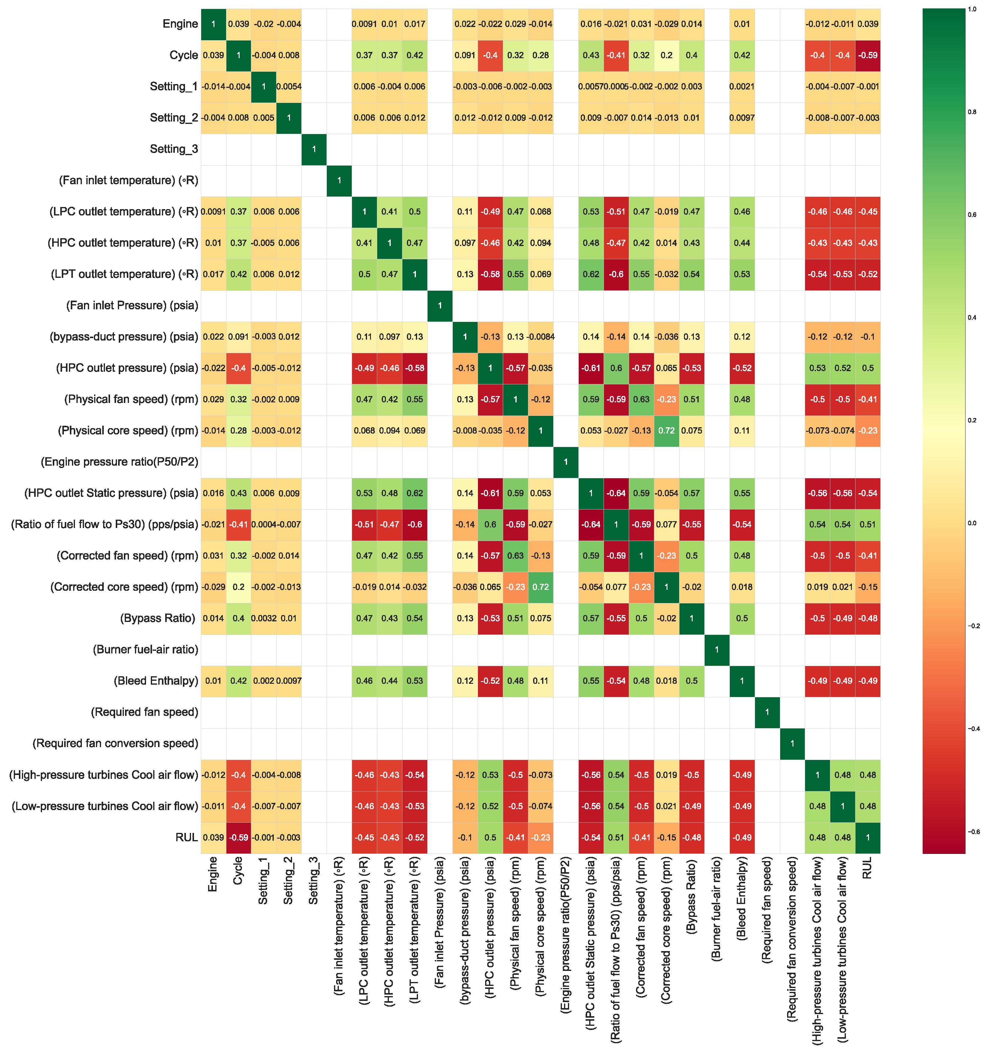
The attributes Setting_3, Fan inlet temperature (°R), Fan inlet pressure (psia), Engine pressure ratio (P50/P2), Burner fuel-air ratio, Required fan speed, and Required fan conversion speed were removed because they remained constant throughout the entire dataset. Due to this lack of variability, these attributes do not contribute relevant information for the RUL estimation model, and retaining them could negatively impact training efficiency. Additionally, Corrected core speed (rpm) was removed due to its high correlation $\left(0.96\right)$ with another attribute, making it redundant for the model, as shown in Figure 3.

Among these, the attributes Setting_1, Setting_2, and Bypass-duct pressure (psia) were removed due to their low correlation with RUL. Since these attributes do not provide significant information for predicting the remaining useful life, their exclusion helps optimize the model’s performance by reducing noise and improving prediction accuracy. Although the Engine column appears as a candidate for removal, it is retained solely for identifying which engine the cycles belong to.

Based on these analyses, attributes with constant values, those with low impact on the target variable, and those with high correlation to other attributes were removed to avoid redundancy and prevent model overfitting. As a result, the training and testing datasets were reduced to 14 attributes: T24, T30, T50, Ps30, Nf, Nc, Ps30, phi, NRf, BPR, htBleed, W31, and W32.

3.1.2. Time-Series to Image Conversion

This section details the transformation of time-series data into a structured format suitable for generative modeling.

Figure 4a presents the normalized sensor signals from the first engine, covering 192 cycles. Figure 4b displays the results after applying Principal Component Analysis (PCA), where the three principal components have been retained. Both figures illustrate how the different signals evolve over time, either increasing or decreasing depending on the cycle, thereby capturing the dynamic behavior of the sensors.

Figure 5a illustrates the processing of a 32-cycle segment. Initially, each segment was represented as a 4 × 8 × 3 pixel structure, where the three PCA components were mapped to the RGB channels. To meet the input size requirements of the generative model, these images were resized to 512 × 512 × 3 pixels, resulting in an initial dataset of 598 images. These images reveal clear trends in the data distribution, as shown in Figure 5b. Notably, as the sequence progresses, the images take on a more reddish hue, indicating an increase in signal intensity as the system approaches failure. This visual representation enhances interpretability, making it easier to identify early failure patterns. The effect is particularly evident in the fifth image, where the intensified coloration suggests an early indication of the system entering a critical state.

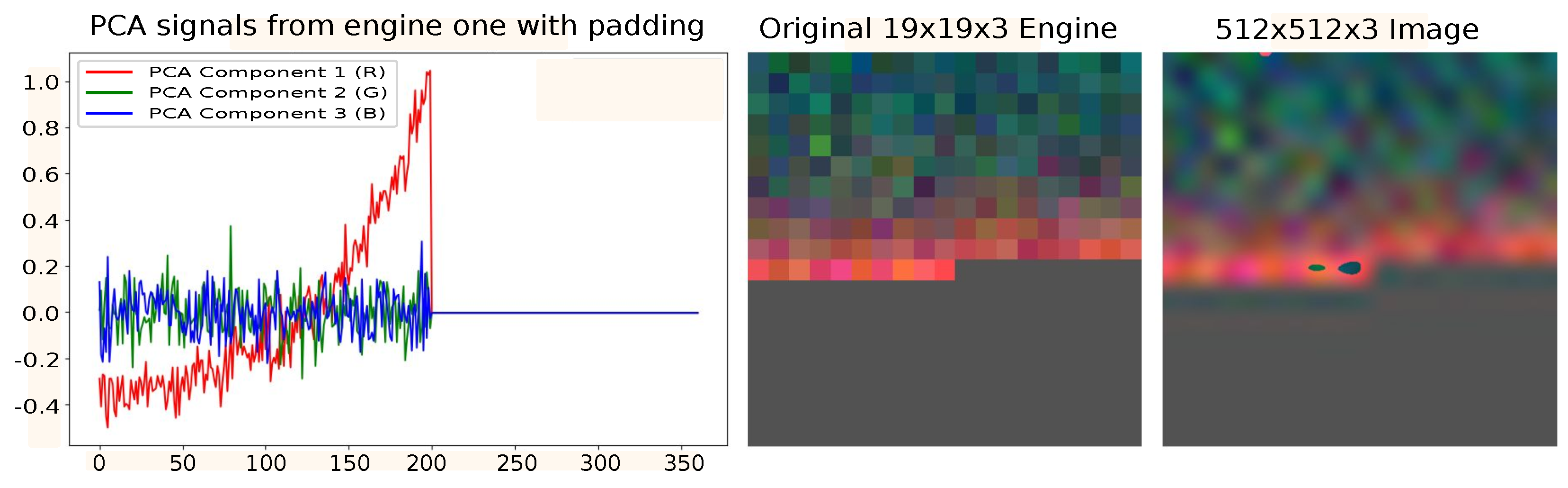
An alternative approach for data representation was also explored, where entire engine signals were used instead of segmented windows. Figure 6 illustrates this process. In this case, the engine with the longest sequence (361 cycles, slightly reduced from 362 for uniformity) was selected as a reference. To ensure consistency across all engines, shorter sequences were padded with additional values (such as zeros) to match the length of the reference engine.

This transformation resulted in a dataset of 100 images, ensuring a consistent visual representation of the signals across different engines. The rightmost image in Figure 6 highlights a key advantage of this representation: its greater intuitiveness compared to the segmented approach, as it preserves the overall signal structure. Additionally, it facilitates the identification of failure indicators over time, as evidenced by the progressive intensification of colors shifting toward reddish tones.

3.1.3. Text Prompts

For the first dataset, each prompt was created using the following template: “(TRIGGER) engine (ENGINE ID), segment (SEGMENT NUMBER)”. Here, TRIGGER represents the unique keyword (not present in the original training of the conditional DDPM) that indicates the concept related to the images, ENGINE ID is the engine identifier, and SEGMENT NUMBER refers to the segment number to be generated. For example, the prompt for the first segment of the first engine would be “CMAPSSS image of engine 1, segment 1”.

For the second dataset, the template was modified to “(TRIGGER) engine (ENGINE ID), cycle (CYCLE NUMBER)”. In this case, the reference to the segment was removed and replaced by the cycle, where CYCLE NUMBER refers to the maximum cycle number of an engine. For example, for the first engine with 192 cycles, the prompt would be “CMAPSSS image of engine 1, cycle 192”.

This step was crucial to ensure that the created data retained the correct category, guaranteeing coherent learning in the generative model. The categories represent different engine states that the model must learn; in the first dataset, the model learns by segments, while in the second, it learns by cycle numbers. Each approach reflects specific aspects of engine operation at different moments.

3.2. Data Generation

In this section, the process of generating synthetic data is specified. Section 3.2.1 describes how the pretrained SD2 models are fine-tuned. Section 3.2.2 analyzes the performance of the fine-tuned models. Next, Section 3.2.3 explains how the selected model is used to generate the final samples that will be used during the experimentation phase.

3.2.1. Fine-Tuning Process

All training experiments were conducted using two NVIDIA Tesla V100 GPUs, each equipped with 16 GB of dedicated memory. Input images were maintained at a resolution of 512 × 512 pixels, despite the SD2 repository recommending 768 × 768 pixels. This decision was made to optimize memory efficiency and simplify the training process while ensuring that the model could effectively process images at the chosen resolution.

The first fine-tuned model was trained for 500 steps, completing the process in approximately 10 minutes. A second model was trained using the same parameter configuration, completing training in approximately 8 minutes. Both models have been uploaded to the Hugging Face repository and are publicly accessible (https://huggingface.co/lpmora/sd2-1-cmapss-dreambooth-lora-rgb-v2 (accessed on 29 April 2025), https://huggingface.co/lpmora/sd2-1-cmapss-dreambooth-lora-rgb-v4 (accessed on 29 April 2025)).

3.2.2. Evaluating the Trained Models

Multiple images were generated, for the first approach, using prompts derived from the specified template. The ENGINE ID and SEGMENT NUMBER values were adjusted as required to explore different configurations. Unfortunately, the results fell short of expectations, indicating that further adjustments or refinements might be necessary.

As shown in Figure 7, the model was expected to generate images resembling the originals, showing a smooth transition from a dark greenish hue to an intense red—indicating a progression toward a critical state. However, the first model generated images with a markedly different color distribution, dominated by brown tones. This inconsistency suggests that the model failed to effectively capture the color variations critical for representing the progressive states of the engine. As a result, interpreting the engine’s condition based on these outputs could be compromised.

The underlying issue could stem from the dataset’s complex and uncommon distribution, characterized by unique color patterns or combinations. During SD2 training, the model may have encountered few or no examples resembling the specific features of the current dataset, such as its distinctive combination of colors and shapes. This limitation likely hindered the model’s ability to generalize effectively. Consequently, this model was deemed unsuitable and discarded for subsequent experiments.

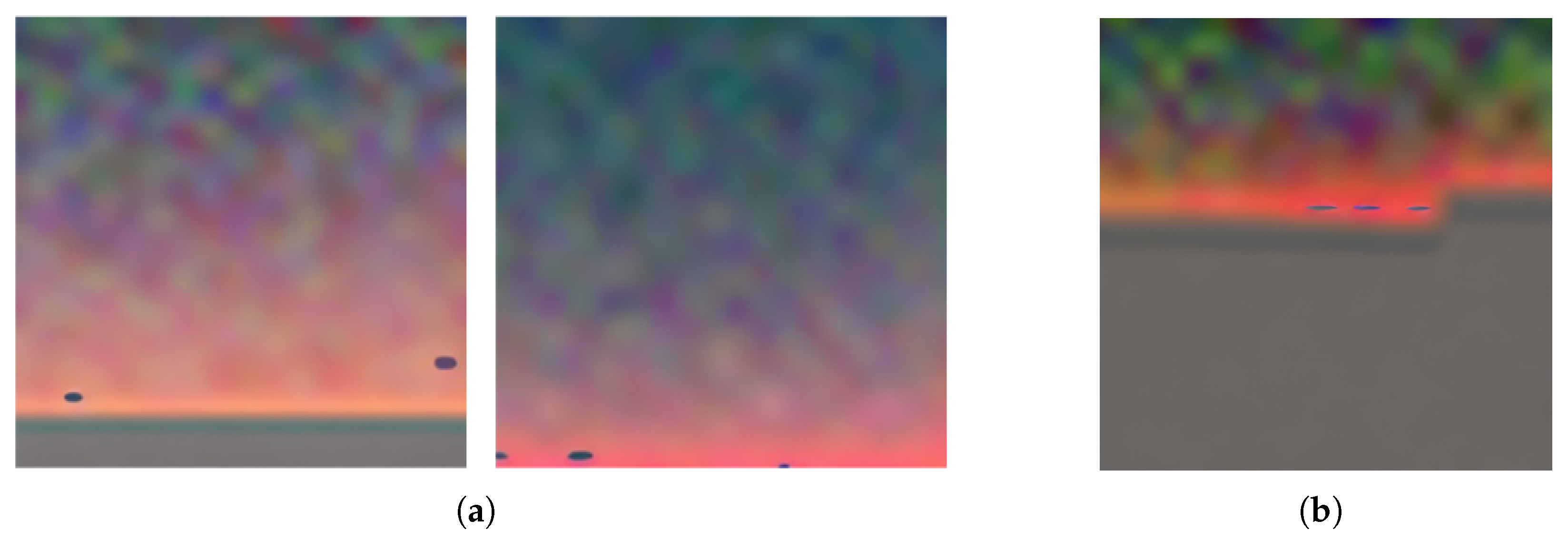
Figure 8a displays an example of data generation with the second approach. The color distribution in the generated images closely matches that of the originals. Greenish tones dominate the upper portion, gradually transitioning into more vibrant reds in the lower portion, as expected. This indicates that the model effectively learned to replicate the desired progression of color patterns.

Furthermore, Figure 8b demonstrates the model’s ability to generate the “broken lines” seen in Figure 6, where part of the last line is interrupted, signifying the end of the cycle. This behavior highlights the model’s capacity to capture specific and intricate details from the training dataset, suggesting a higher level of fidelity to the data’s unique characteristics.

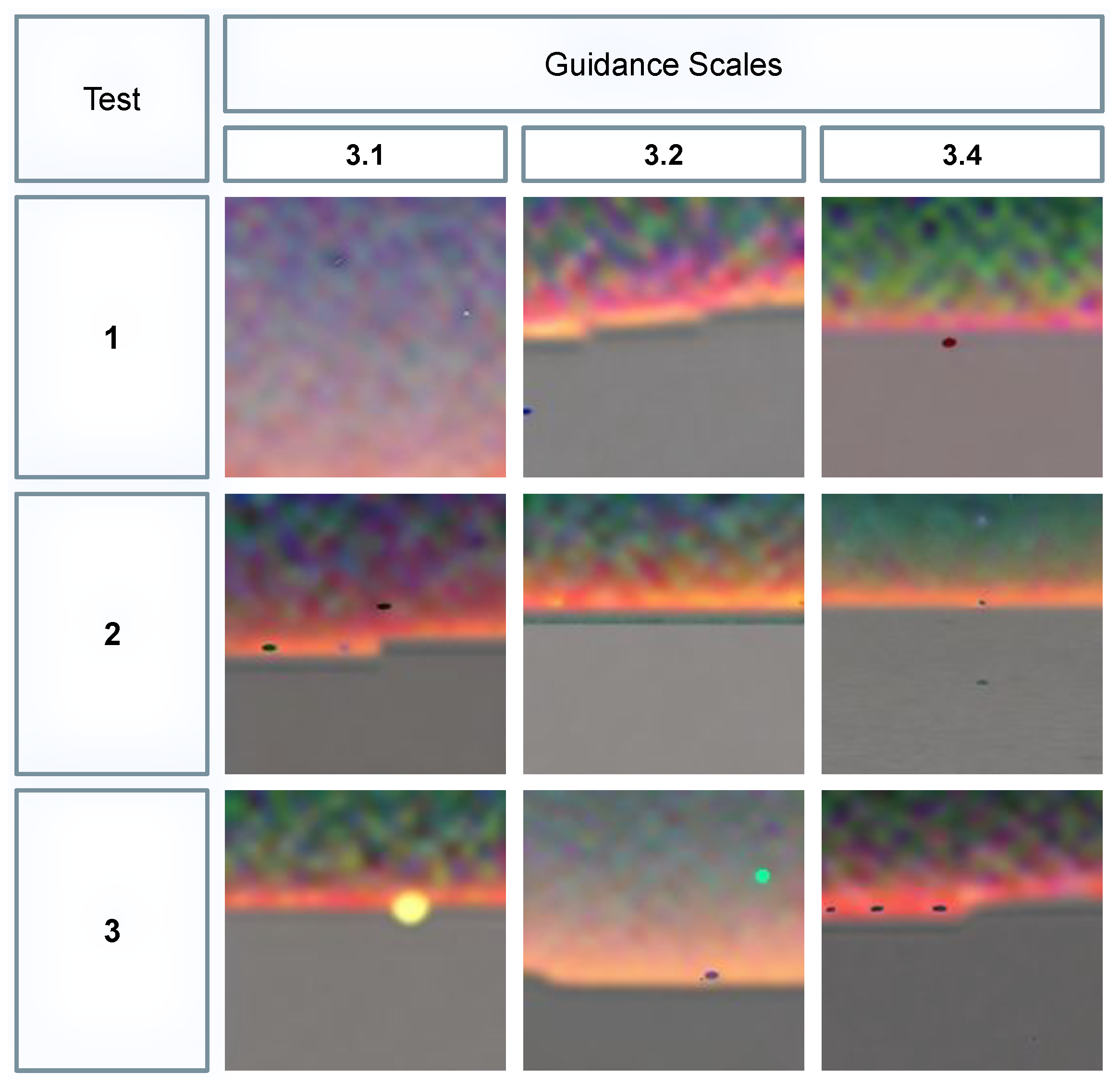
One of the most critical parameters during image inference was the guidance scale, as it significantly impacted the quality and accuracy of the generated images. This parameter determines the balance between the model’s creativity and its adherence to the provided descriptions. Properly tuning this value is essential for achieving optimal results. If the guidance scale is set too low, the model generates images that closely resemble the training set, limiting diversity. Conversely, if the value is too high, the generated images may diverge excessively and lack relevance to the original inputs.

To identify the optimal balance, multiple experiments were conducted by adjusting the guidance scale across a range of values from 1 to 10. The results showed that the most effective values were 3.1, 3.3, and 3.4, striking a suitable balance between fidelity and creative variation.

Figure 9 illustrates the results obtained from various tests using the most effective guidance scale values:

• First Test: At a guidance scale of 3.1, the model failed to accurately follow the prompt, generating colors that diverged from the originals. With 3.2, the lines were inconsistent, either not entirely straight or with missing segments. However, at 3.4, the model produced straight lines but generated more lines than were specified in the prompt.
• Second Test: At 3.1, there was noticeable improvement, yet the model still produced more lines than required, failing to fully align with the prompt. At 3.2, while the lines were straight, the excess persisted. With 3.4, the model managed to produce straighter lines in the correct quantities, better matching the expected output.
• Third Test: At 3.1, the model introduced a yellowish spot resembling a sun during sunrise or sunset, though it successfully generated fewer, straighter lines. At 3.2, the colors were overly faint, the model produced too many lines, and the last one appeared incomplete—failing to meet the requirement for continuous lines. At 3.4, the model produced unbroken lines with appropriate colors, though some imperfections in straightness remained.

Based on these observations, a guidance scale of 3.4 was selected as the optimal setting. It struck the best balance between creativity and adherence to the training data, producing results that were closest to the expected outputs overall.

One of the primary challenges encountered was the model’s inability to effectively follow the prompt. As observed during the guidance scale tests, the generated images often featured an incorrect number of lines that did not align with the cycle signals from the training data. This limitation may stem from the model’s difficulty in associating textual descriptions with visual representations. Addressing this issue may require refining the script or leveraging a more advanced model to enhance its interpretive capabilities.

Interestingly, some of the generated images bore a striking resemblance to landscapes, starry skies, or sunsets, with textures evocative of oceans or horizons. In the guidance scale tests, five out of nine images displayed straight lines, a pattern that might be explained by the model’s interpretation of horizons present in the dataset.

3.2.3. Data Preparation

Since the second model generated images similar to the originals, 100 synthetic images were created to match the number of samples in the original dataset and assess their quality for expanding the CMAPSS dataset.

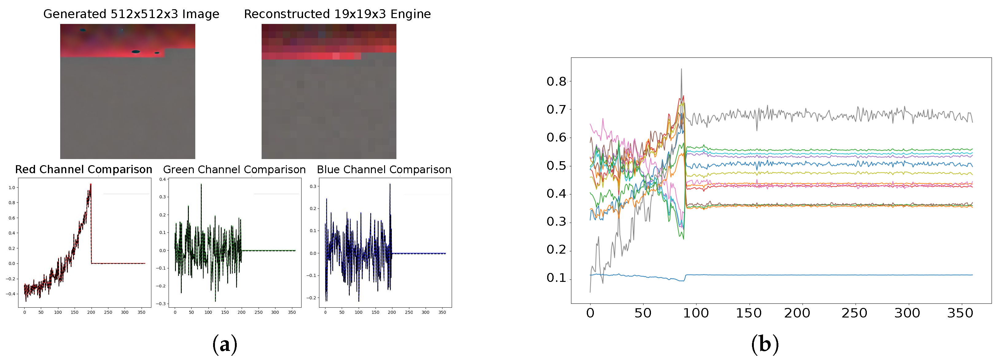
Once the 100 images were generated and validated, the steps described in Section 2.4 were applied. Figure 10 illustrates the results of the described process. Figure 10a shows the images and graphs of the three components: first in their generated form and then reconstructed into time-series. In the lower graphs, the three components corresponding to the RGB channels are represented as colored lines, depicting the reconstructed components for the first engine with 128 cycles and padding. Figure 10b displays the result of applying the inverse PCA. These signals were adjusted to replicate the behavior of engine one and, after processing, exhibit a high degree of similarity to the original engine data, successfully achieving the desired outcome. The graph demonstrates how the trend toward failure has been accurately replicated, with signals rising or falling based on the sensor type, indicating that the model has effectively learned to generate consistent and realistic data.

Figure 11 presents the final result of the generated signals, now without padding. Since the model did not strictly adhere to the prompt, the generated data did not exactly match the specified 128 cycles. After removing the padding, 89 cycles were obtained, resulting in new samples that were not part of the original dataset.

3.3. Experimentation Setup

This section presents the experiments conducted to assess the performance of Remaining Useful Life (RUL) estimation models using three types of datasets: original data, synthetic data, and a combination of both. The primary objective is to compare model performance, identify the dataset that yields the most accurate predictions, and evaluate whether augmenting the dataset with synthetic data enhances predictive accuracy beyond that achieved with the original dataset alone.

To quantify the impact of synthetic data, the results are benchmarked against a baseline model, selected based on a prior comparative analysis of three models from the literature.

Furthermore, the study explores the relationship between dataset size and the proportion of synthetic data used, assessing their combined effect on model performance and generalization.

For this task, a hybrid model integrating Long Short-Term Memory (LSTM) networks and Convolutional Neural Networks (CNNs) was employed. This architecture was chosen due to its ability to leverage the strengths of both approaches; LSTMs excel at capturing temporal dependencies, such as engine wear trends, while CNNs effectively extract key features, including sensor-specific patterns. The synergy between these methods enhances the model’s ability to manage the complexities of RUL prediction [27,28].

The implemented architecture consists of an initial 1D convolutional layer with 64 filters and ReLU activation, followed by a MaxPooling layer to reduce dimensionality and prevent overfitting. Next, a second 1D convolutional layer with 32 filters is applied, followed by an LSTM layer with 100 units to capture temporal relationships in the data. To further mitigate overfitting, a Dropout layer with a 20% rate is incorporated. Finally, a dense output layer with a single unit is used to generate the final prediction. The model is compiled using the Adam optimizer with a learning rate of 0.001, and the mean squared error (MSE) loss function is employed.

During training, the model processes the original dataset along with target attribute labels, using fixed-length sequences of 32 data points.

The training process spans 45 epochs with a batch size of 256, yielding a trained model alongside a loss history that tracks performance across all epochs.

To mitigate the impact of excessively high values on the training process, the RUL target attribute is capped at a maximum value of 130. This constraint ensures that the model prioritizes learning the most relevant degradation patterns while improving its generalization capability.

Each experiment is repeated 10 times to ensure the reliability and robustness of the results, reducing the impact of random variations and enhancing the statistical significance of the findings.

4. Results

This section presents the results of evaluating remaining useful life (RUL) estimation models using original, synthetic, and combined data. It outlines the configuration settings, evaluation metrics, and test scenarios, comparing the results with a baseline model to assess the impact of synthetic data on prediction accuracy.

4.1. Baseline

Firstly, the CNN-LSTM model was trained using 100% of the original dataset. The results were also compared with the findings of Wang et al. [29] and Sharma et al. [30] from their respective studies.

The performance of the model was assessed using the Mean Absolute Error (MAE), Root Mean Squared Error (RMSE), and R² Score (coefficient of determination) metrics. The R² Score is a widely used metric in regression models that measures how well the predictions align with actual outcomes or validate a given hypothesis. In this study, it was specifically applied to evaluate the model’s accuracy in predicting the Remaining Useful Life (RUL).

Table 2. Performance comparison between the CNN-LSTM model and the LSTM models proposed by Vinayak and Carl.

Metric	CNN-LSTM Model	Bi-LSTM Model [29]	TCN [30]	Improvement vs. [29] (%)	Improvement vs. [30] (%)
MAE ↓	11.75	–	18.75	–	37.33%
RMSE ↓	14.76	18.85	26.56	21.16%	44.43%
R2 Score ↑	0.87	–	0.84	–	4%

presents the results of the proposed CNN-LSTM model. The findings demonstrate a significant improvement across all metrics, particularly in the MAE and RMSE metrics, with improvements exceeding 20%.

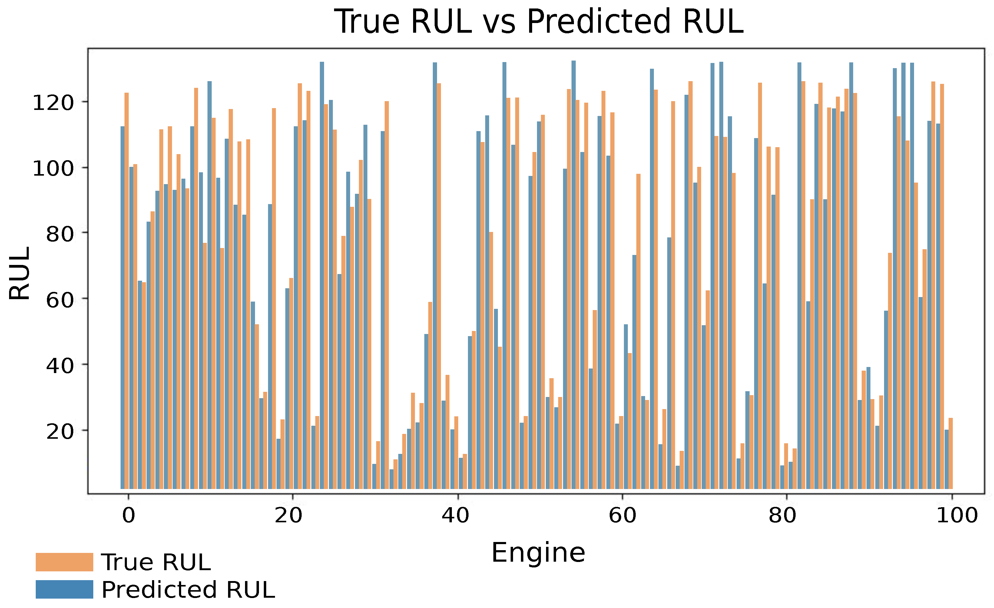
A comparative plot was generated between the actual and predicted RUL values, illustrating that the predictions closely follow the trend of the actual values, with only minor deviations observed in certain cases.

Figure 12 presents a comparison between the actual RUL (blue line) and the predicted RUL (orange line) for the engines in the test dataset. Overall, the model effectively captures the trends of the actual RUL, with both lines aligning closely in many sections. However, some fluctuations and deviations are observed at specific points, where the predictions either overestimate or underestimate the RUL for certain engines.

Despite these inconsistencies, the model demonstrated satisfactory performance in capturing the overall RUL trend.

4.2. Analysis of the Size of the Dataset and the Amount of Synthetic Data

To evaluate the performance of this approach, we conducted a series of experiments using different training configurations. The objective was to analyze how the inclusion of synthetic data affects model accuracy across various dataset sizes and training epochs. The experiments were conducted using datasets of three different sizes: 25, 50, and 100 samples. To assess the impact of synthetic data, we considered three configurations: training on purely original data (0% synthetic), training with 25% synthetic data, and training with 50% synthetic data.

Each model configuration was trained for 45, 75, and 100 epochs to study the effect of prolonged training on performance. To ensure robustness, we repeated each experiment 10 times and reported the mean and variance of each metric across these runs.

The results of our experiments are presented in

Table 3. Comparison of MAE (Mean Absolute Error) and its variance across different sample sizes, training epochs, and synthetic data proportions, including 0% synthetic data.

Epochs	Synthetic Data	MAE ± Variance
		25 Samples	50 Samples	100 Samples
45	0%	35.49 ± 10.44	15.57 ± 26.63	10.53 ± 0.27
	25%	34.16 ± 26.65	14.32 ± 0.26	11.28 ± 0.63
	50%	29.75 ± 34.78	12.92 ± 0.72	11.43 ± 0.17
	75%	26.20 ± 43.77	13.34 ± 1.81	11.53 ± 0.26
	100%	22.91 ± 41.76	13.49 ± 2.17	11.28 ± 0.27
75	0%	17.33 ± 38.73	11.22 ± 0.42	10.40 ± 0.61
	25%	16.90 ± 13.80	11.59 ± 0.74	11.38 ± 0.66
	50%	20.73 ± 86.63	13.02 ± 1.83	11.10 ± 0.79
	75%	17.20 ± 44.95	12.49 ± 0.37	11.33 ± 0.82
	100%	19.14 ± 83.06	12.26 ± 1.31	11.41 ± 0.42
100	0%	14.80 ± 49.31	11.07 ± 0.63	10.46 ± 0.18
	25%	13.79 ± 0.96	14.18 ± 51.78	11.38 ± 0.66
	50%	15.26 ± 5.48	12.29 ± 0.68	11.10 ± 0.79
	75%	13.94 ± 0.49	12.40 ± 0.37	11.33 ± 0.82
	100%	15.57 ± 29.20	12.26 ± 1.31	11.41 ± 0.42

,

Table 4. Comparison of RMSE (Root Mean Squared Error) and its variance across different sample sizes, training epochs, and synthetic data proportions, including 0% synthetic data.

Epochs	Synthetic Data	RMSE ± Variance
		25 Samples	50 Samples	100 Samples
45	0%	39.46 ± 9.15	19.27 ± 31.76	14.03 ± 0.23
	25%	38.12 ± 15.32	18.52 ± 0.44	14.88 ± 0.71
	50%	34.87 ± 21.87	16.93 ± 0.68	14.92 ± 0.35
	75%	32.44 ± 28.93	17.34 ± 1.39	15.03 ± 0.43
	100%	28.98 ± 27.56	17.55 ± 1.73	14.88 ± 0.41
75	0%	21.61 ± 43.48	14.73 ± 0.30	14.17 ± 0.61
	25%	21.10 ± 12.40	15.18 ± 0.67	14.99 ± 0.63
	50%	24.80 ± 69.12	16.72 ± 1.53	14.63 ± 0.77
	75%	21.65 ± 38.44	15.93 ± 0.34	14.87 ± 0.78
	100%	23.49 ± 64.10	15.68 ± 1.12	14.94 ± 0.39
100	0%	18.62 ± 55.87	14.86 ± 0.59	14.12 ± 0.30
	25%	17.73 ± 0.81	17.23 ± 45.34	14.99 ± 0.63
	50%	19.18 ± 4.42	15.85 ± 0.61	14.63 ± 0.77
	75%	17.88 ± 0.67	15.90 ± 0.34	14.87 ± 0.78
	100%	19.32 ± 25.77	15.68 ± 1.12	14.94 ± 0.39

and

Table 5. Comparison of $R^2$ scores and their variance across different sample sizes, training epochs, and synthetic data proportions, including 0% synthetic data. Higher values are better.

Epochs	Synthetic Data	${\mathit{R}}^2$ ± Variance
		25 Samples	50 Samples	100 Samples
45	0%	0.05 ± 0.02	0.76 ± 0.03	0.88 ± 0.00
	25%	0.07 ± 0.05	0.78 ± 0.01	0.87 ± 0.01
	50%	0.12 ± 0.07	0.80 ± 0.02	0.86 ± 0.01
	75%	0.18 ± 0.09	0.79 ± 0.03	0.85 ± 0.02
	100%	0.24 ± 0.08	0.78 ± 0.02	0.86 ± 0.01
75	0%	0.69 ± 0.05	0.87 ± 0.00	0.88 ± 0.00
	25%	0.70 ± 0.04	0.88 ± 0.01	0.86 ± 0.02
	50%	0.64 ± 0.08	0.85 ± 0.02	0.87 ± 0.01
	75%	0.67 ± 0.06	0.86 ± 0.02	0.86 ± 0.01
	100%	0.65 ± 0.07	0.86 ± 0.01	0.86 ± 0.01
100	0%	0.76 ± 0.07	0.87 ± 0.00	0.88 ± 0.00
	25%	0.78 ± 0.06	0.85 ± 0.03	0.86 ± 0.02
	50%	0.75 ± 0.04	0.86 ± 0.02	0.87 ± 0.01
	75%	0.77 ± 0.05	0.86 ± 0.01	0.86 ± 0.01
	100%	0.74 ± 0.06	0.86 ± 0.01	0.86 ± 0.01

, where we report the mean and variance for MAE, RMSE, and $R^2$ across different configurations.

The impact of synthetic data varies depending on the available sample size. When working with a small number of samples, synthetic data can sometimes improve the mean absolute error (MAE and RMSE), although it may also lead to increased variance. With a moderate number of samples, the best performance is generally obtained with either no synthetic data or a balanced proportion. For larger datasets, the benefits of synthetic augmentation tend to diminish, as training exclusively on real data often yields the lowest MAE.

The number of training epochs significantly influences the performance. In general, increasing the number of epochs results in lower MAE, as the model benefits from extended training. However, the effect of synthetic data varies across different epoch settings. While high proportions of synthetic data can be beneficial in early training stages, the optimal strategy changes as training progresses, with lower synthetic data proportions yielding better results in later epochs.

Stability is another crucial aspect when assessing model performance. High variance in certain configurations suggests inconsistent results across different runs, whereas lower variance indicates greater reliability. Beyond minimizing MAE, ensuring stability is essential for robust model evaluation. The balance between real and synthetic data must be carefully considered, as synthetic augmentation is more beneficial when real data are scarce, while models trained on sufficient real data tend to perform better without additional synthetic samples.

The $R^2$ values remained stable across configurations, indicating that synthetic data did not introduce significant bias but also did not contribute strongly to further performance gains when sufficient real data were present.

5. Discussion

The results obtained in this study highlight the impact of synthetic data on model performance, particularly in scenarios with limited real samples. The inclusion of synthetic data demonstrated potential benefits in improving model accuracy during the initial training phases, especially when real data availability was low. However, as the number of real samples increased, the advantage of synthetic data diminished, suggesting that their primary role is to provide meaningful augmentation in data-scarce situations. Furthermore, the variance in the results indicates that while synthetic data can help reduce error, they may also introduce instability depending on the proportion used and the number of training epochs.

Compared to existing approaches that rely solely on real data or employ traditional augmentation techniques such as noise injection and geometric transformations, the proposed method—based on synthetic data generation using a conditional Denoising Diffusion Probabilistic Model (DDPM)—offers greater flexibility for data expansion. Unlike standard augmentation methods, which apply predefined perturbations to existing samples, our approach synthesizes entirely new instances, capturing complex and realistic variations beyond simple transformations.

Previous studies have shown that generative models such as GANs and VAEs can improve model generalization; however, diffusion models offer a more stable training process and are capable of producing higher-quality samples. Our findings are consistent with these observations, especially in low-data regimes, where synthetic data improve model performance without introducing significant artifacts. This study highlights the strong potential of DDPMs for data augmentation, in line with recent research [11,31,32].

The effect of training duration was also analyzed, revealing that increasing the number of epochs generally led to improved performance across different data configurations. However, the interaction between synthetic data and training duration was not uniform, with some configurations benefiting more than others. This suggests that optimizing the balance between real and synthetic data requires consideration of both dataset size and training duration. Additionally, the observed variance highlights the importance of not only focusing on mean performance metrics but also ensuring model stability, as excessive fluctuations can undermine the reliability of the generated results.

Beyond performance metrics, the study underscores the importance of selecting appropriate preprocessing techniques and model configurations when integrating synthetic data. While existing approaches often apply synthetic data in fixed proportions, our findings suggest that an adaptive strategy may be more effective. Future research should explore dynamic adjustments to synthetic data proportions based on training progress and model convergence.

Furthermore, investigating alternative data generation techniques, such as hybrid approaches combining diffusion models with other generative frameworks, could enhance robustness and further improve generalization capabilities. In particular, the use of autoencoders (AEs) as a dimensionality reduction method represents a promising direction. Future work may include a comparative study between PCA-based and AE-based transformations, evaluating their respective impacts on downstream performance in image-based learning architectures.

In addition to the bias introduced by evaluating the method primarily under data-scarce conditions and the observed variance in the results, another important limitation is the computational demand of the proposed approach. While diffusion models are effective in generating high-quality synthetic data, they require significant computational resources and extended processing times. This constraint may hinder the deployment of the method in real-time or resource-constrained environments, particularly in industrial settings where rapid decision making is critical.

Furthermore, the performance of the model may depend on the quality, expressiveness, and consistency of the textual prompts used for conditioning. Inaccurate or ambiguous descriptions could negatively impact the relevance and fidelity of the generated data. Lastly, the generalizability of the proposed method to a broader range of real-world failure modes, beyond those present in the training data, remains an open question and warrants further investigation in future work.

6. Conclusions

In this work, we explored the integration of synthetic data in training models for scenarios with limited real data. Our analysis demonstrates that synthetic data can reduce MAE and RMSE when the available dataset is small, offering a means to supplement scarce real data. However, the benefits of synthetic augmentation are not uniform; as the sample size increases, the performance gains diminish, and models trained solely on real data often exhibit superior results.

The study also highlighted the importance of training duration. Extended training through more epochs generally improves model performance, reducing error as the model learns more robust features. Nevertheless, the influence of synthetic data varies over time. While high proportions of synthetic data can be beneficial during early epochs by enhancing diversity and accelerating convergence, a lower synthetic data ratio seems to be optimal in later stages of training.

Overall, our findings underscore the need to balance error reduction and model stability when employing synthetic data. The early infusion of synthetic samples can be a powerful strategy to counteract the limitations of small datasets, but a dynamic approach may be required to adjust the balance between synthetic and real data as training progresses. Future work may further investigate adaptive techniques that optimize this balance to enhance both the accuracy and stability of models in various data-scarce environments.