Article

Mechanical Fault Diagnosis Method of a Disconnector Based on Improved Dung Beetle Optimizer–Multivariate Variational Mode Decomposition and Convolutional Neural Network–Bidirectional Long Short-Term Memory

by
Chi Zhang
,
Hongzhong Ma
* and
Wei Sun
School of Electrical and Power Engineering, Hohai University, Nanjing 211100, China
*
Author to whom correspondence should be addressed.
Machines 2025, 13(4), 332; https://doi.org/10.3390/machines13040332
Submission received: 16 March 2025 / Revised: 12 April 2025 / Accepted: 16 April 2025 / Published: 18 April 2025
(This article belongs to the Section Machines Testing and Maintenance)

Abstract

:
As one of the main faults of a disconnector, a mechanical fault is difficult to diagnose in time because of its weak self-evidence, its wide range of fault categories, and the difficulty in obtaining fault sample data. To address this issue, this study proposes a new fault diagnosis algorithm based on multivariate variational mode decomposition optimized by the improved dung beetle optimizer, and at the same time, an experimental platform for vibration signal acquisition was built to simulate three typical mechanical faults. First, the parameters of multivariate variational mode decomposition were optimized using an improved dung beetle optimizer, and the intrinsic mode function with a Pearson correlation coefficient higher than 0.1 was retained after the signal was decomposed. Then, the energy, entropy, and time–frequency domain eigenvalues of the selected intrinsic mode function were calculated to construct the feature matrix, and its dimensions were reduced to two dimensions. Finally, this matrix was input to convolutional neural network–bidirectional long short-term memory for fault classification. The verification of the experimental data shows that the proposed algorithm can successfully diagnose different mechanical faults of the disconnector, and the accuracy rate was 96.67%. The research content provides a new idea for the fault diagnosis of disconnectors.

1. Introduction

Disconnectors are the most widely used switch equipment and play a key role in power systems [1,2,3,4]. In engineering practice, disconnectors work outdoors for a long time and are inevitably affected by the working environment, resulting in a series of mechanical failures. Taking 30 substations with a voltage level of 220 kV in the southern area of a city as an example, the statistical data show that there were 160 defects in the disconnector between 2020 and 2024, accounting for the highest proportion of all kinds of substation main equipment, among which mechanical faults accounted for more than 53%. From the perspective of mechanical structure dimension, the total defect rate of horizontal two-column (GW4) disconnector is the highest, accounting for more than 50%. It can be seen that mechanical failure is the main fault of the disconnector. The mechanical faults of a disconnector mainly include mechanism jam, mechanism looseness, and three-phase asynchrony [5,6,7]. Disconnectors work outdoors and are easily affected by the environment such as wind, acid rain, and ultraviolet radiation, and the transmission mechanism is prone to accumulate dust or rust, leading to mechanism jam failures. If it cannot be cleaned in time, the degree of jam will gradually increase, and in severe cases, it will lead to mechanism fracture. After multiple operations, the bolt of the mechanism will loosen, leading to abnormal vibration of the disconnectors and affecting its normal operation. The disconnector has an adjustable connecting rod, and during the installation and commissioning of the disconnector, improper operation of the staff or the vibration generated during the operation will lead to improper adjustment of the connecting rod, resulting in abnormal positions of the components and, in severe cases, damage to the connecting rod [8,9,10].
Owing to limitations in manufacturing processes and monitoring conditions, the mechanical failure rate of disconnectors remains high [11]. According to current research, the mechanical fault diagnosis of disconnectors mainly includes two aspects: feature extraction and fault identification. From the perspective of feature extraction, the vibration signal reflects the operating state of the disconnector and has become the mainstream feature signal for disconnector fault diagnosis [12]. Compared to spindle angle signals, torque signals, and motor current signals, the frequency characteristics and periodicity of the vibration signal are clearer [13]. Therefore, signal decomposition methods such as empirical mode decomposition (EMD), short-time Fourier transform (STFT), and variational mode decomposition (VMD) are widely used. Reference [14] used EMD to decompose the vibration signal and extract features. However, when there is no white noise in EMD, modal aliasing often occurs, and the signal cannot be reliably decomposed. Reference [15] used STFT to extract key features, including the peak frequency and amplitude. Reference [16] solved the EMD problem by decomposing a signal using improved VMD.
However, the above signal decomposition method needs to be decomposed one by one when decomposing multiple input data, while multivariate variational mode decomposition (MVMD) can perform modal decomposition on multi-dimensional data, comprehensively consider the relationship between multiple features, increase the effectiveness of signal reconstruction while maintaining the overall structural consistency of the data, and enhance the robustness of decomposition [17]. However, the number of modes K and penalty factor α determine the decomposition impact of the MVMD. In the past, the selection of K and α typically adopted the central frequency observation method, and the results obtained by this method were more random. To improve the reliability of decomposition, the dung beetle optimizer (DBO) is introduced to select the optimal solution of K and α. Inspired by the four social behaviors of the dung beetle population, the DBO algorithm was proposed in 2023 [18]. Reference [19] optimized K and α in VMD using the DBO algorithm for fault identification, and the reasonable selection of K and α also significantly improved the fault identification accuracy. Simultaneously, numerous engineering problems have been solved using the DBO method [20,21]. However, there is still considerable research space in the performance of the DBO algorithm. In order to further improve the accuracy of fault identification, in this study, an improved DBO algorithm was used to optimize the two parameters of MVMD and then optimize the decomposition of vibration signals.
From the perspective of fault identification, owing to the diverse operating characteristics of disconnectors under different operating conditions, it is no longer reliable to identify faults using fixed thresholds or expert scoring systems [22]. At present, recognition methods mainly include k-nearest neighbor (KNN), backpropagation neural network (BPNN), and support vector machine (SVM). These methods have led to significant progress in fault identification. During the actual operation of disconnectors, their early fault characteristics are often not evident, and the operating characteristics of different mechanical faults in a certain period may be similar. The aforementioned shallow learning algorithms can reasonably distinguish relatively obvious faults, but they are often powerless in the face of similar features among several faults, which significantly affects the accuracy of fault recognition [23]. In view of this, a large number of deep learning algorithms have emerged in recent years, which have a higher efficiency in dealing with such problems. Reference [24] used convolutional neural network (CNN) to diagnose faults based on vibration and sound signals in transformers, but it is difficult to capture global information only by CNN. Reference [25] used long short-term memory (LSTM) to detect anomalies in transmission equipment based on voiceprint signals. However, LSTM limits the parallel capability of the model and has the drawback of a longer diagnosis time. Reference [26] used CNN-LSTM for the fault diagnosis of integrated energy systems, but the unoptimized network structure is difficult to train and may even degenerate. With continuous improvements in deep learning algorithms, both CNN and bidirectional long short-term memory (BiLSTM) have demonstrated good stability and high accuracy in data processing and fault diagnosis. CNN-BiLSTM combines the feature learning ability of CNN with the time series memory function of BiLSTM, which can further improve the identification accuracy while improving the computation speed. Therefore, CNN-BiLSTM was selected to identify the fault types of disconnectors in this study, and the specific structure is shown in Figure 1.
On the whole, there are mainly the following problems in the fault diagnosis of disconnectors:
(1)
After the mechanical failure of disconnectors, the state data cannot be obtained, resulting in insufficient sample size of the fault data.
(2)
The actual fault simulation cost of disconnector is high, and the degree and frequency of fault simulation are limited.
(3)
There are many joints in the transmission mechanism of the disconnector, there are many types of mechanical faults, and the fault self-evident is weak.
Therefore, it is of great significance to study the state data acquisition method, feature extraction method, and fault identification method of the disconnector to improve the intelligent operation and maintenance level of disconnector and maintain the stable operation of power supply system.
Considering the aforementioned problems, this study suggests a method for diagnosing mechanical faults in disconnectors based on parameter-optimized MVMD with an improved DBO and CNN-BiLSTM. The main contributions are as follows:
(1)
In order to solve the problem of parameters selection of MVMD, an improved dung beetle optimization algorithm is introduced to better decompose the vibration signals collected in the experiment.
(2)
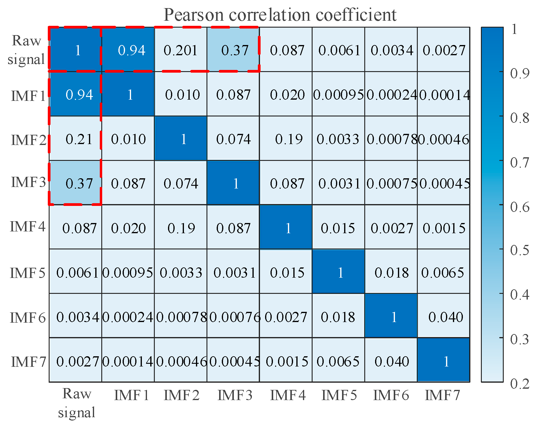
In order to improve the efficiency of feature extraction, the Pearson correlation coefficient is used to select the intrinsic mode function (IMF) with the highest correlation with the original signal, and the eigenvalues of IMFs are calculated from the energy, entropy, and time–frequency domains to construct the fusion feature as the feature matrix. Extracting fault features from multiple domains can solve the problem of weak self-evident mechanical fault of disconnector to a certain extent.
(3)
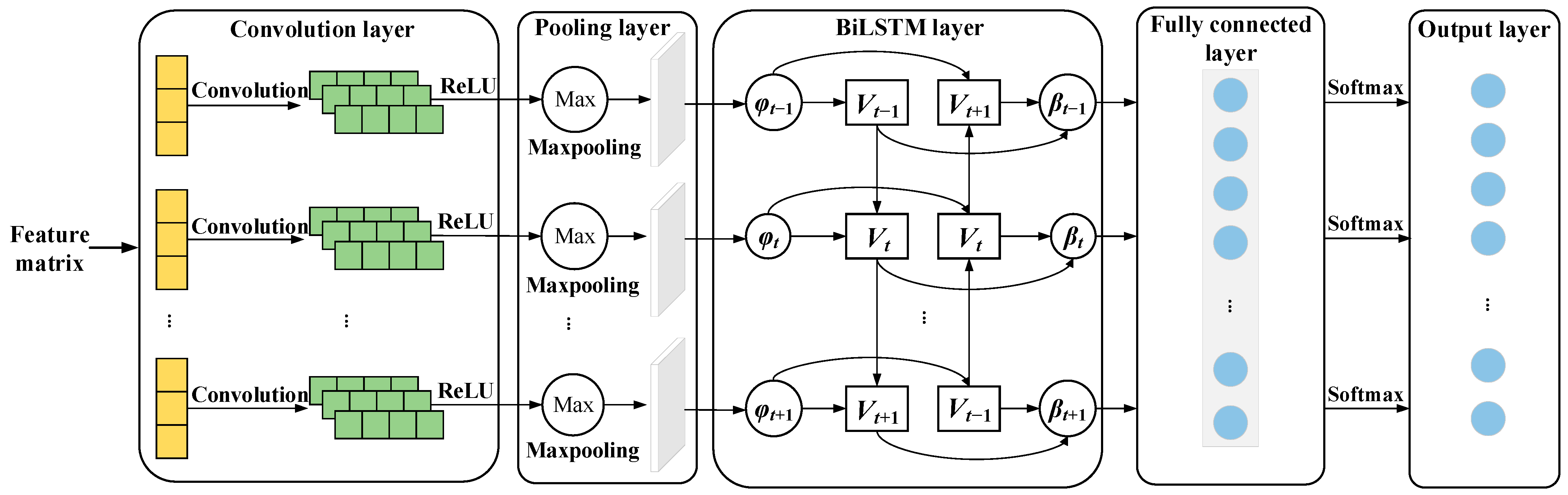
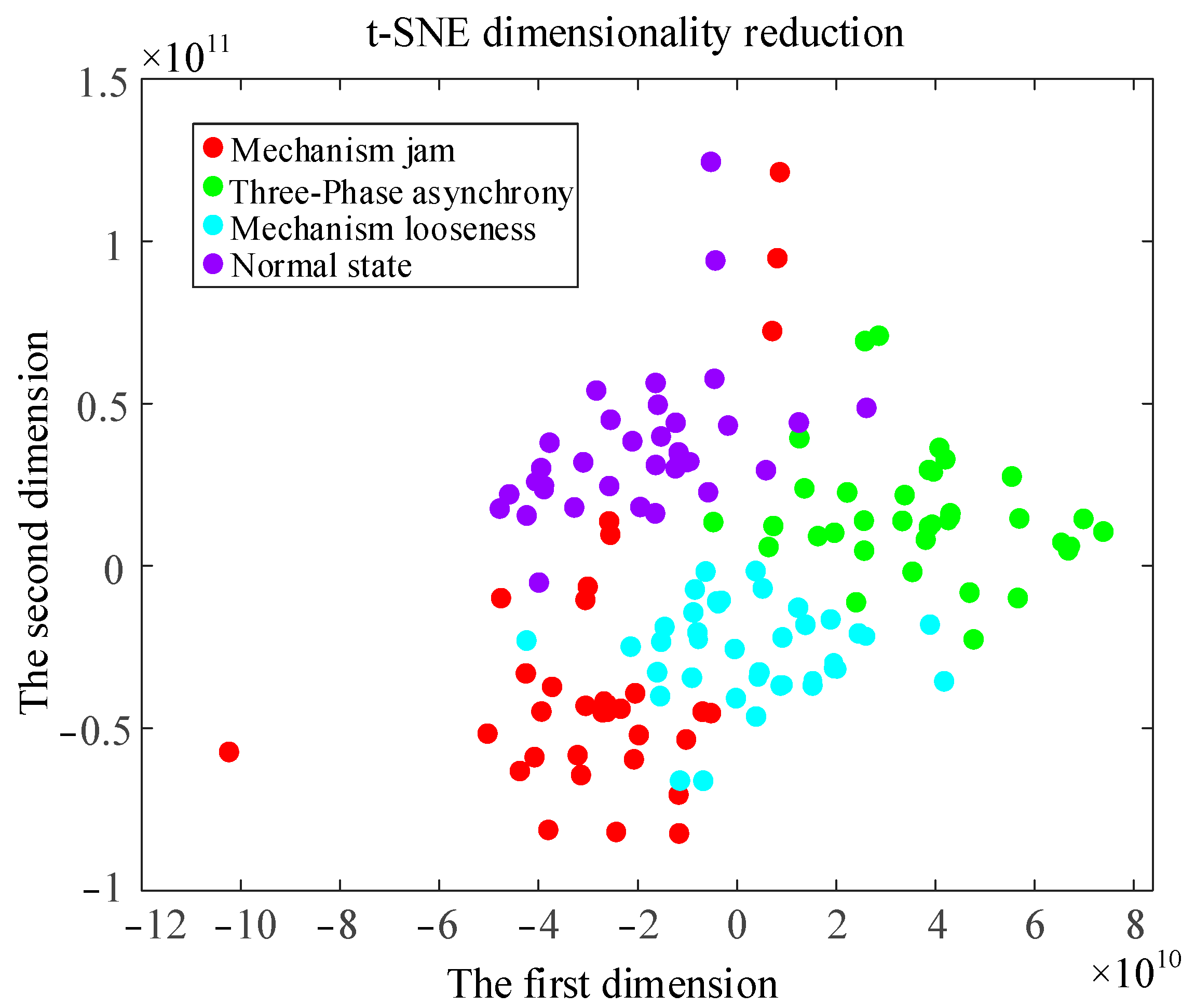
In order to improve the operation speed and recognition accuracy, the dimensions of the feature matrix are reduced to two dimensions using the t-distributed stochastic neighbor embedding (t-SNE) method, and then the processed matrix is input to CNN-BiLSTM to obtain the fault identification results. The CNN-BiLSTM model can accurately distinguish the four operating conditions of the disconnector, and the fault diagnosis rate is high.
(4)
On the premise of controlling the overall cost of the platform, a disconnector fault experimental platform is built. Without destroying the disconnector equipment itself, three typical mechanical faults are innovatively simulated, vibration data under different conditions are collected, and the sample size of fault data is increased. Using the extracted vibration signal data, the usefulness of the constructed model is proved, and the signal variation law under different fault types is discussed.
The next sections of the article are arranged as below: In Section 2, the theoretical processes of MVMD and improved DBO algorithm are presented. In Section 3, the construction of an experimental platform, fault-type simulation, and vibration signal acquisition are described. In Section 4, the data analysis is introduced, and the results of fault diagnosis are discussed. Section 5 summarizes the work done in this study.

2. The Proposed Method

2.1. Multivariate Variational Mode Decomposition

MVMD is a generalized extension of VMD, with the main objective of extracting K predefined multivariate IMFs from a multivariate raw signal x(t):
x ( t ) = k = 1 K u k ( t )
where u k (t) = [ u 1 (t), u 2 (t), ···, u C (t)] represents the kth IMF component after decomposition, and the parameter C represents the number of data channels in x(t), x(t) = [ x 1 (t), x 2 (t), ···, x C (t)].
The analytic vector of u k (t) is represented by u + k (t) and then multiplied by the exponential term to adjust it to the corresponding center frequency ω k (t). Analyzing the norm L2 of the gradient function of u + k (t) allows one to estimate the bandwidth of u k (t), and the MVMD constrained optimization issue is expressed as
min u k , c , ω k k c t u + k , c ( t ) e j ω k t 2 2 s . t . k u k , c ( t ) = x c ( t ) , c = 1 , 2 , , C
where u + k , c represents the analytic representation of each element in the corresponding channel c and vector u k (t), ω k represents the collection of the central frequencies, and t represents the time-dependent partial derivative. The corresponding augmented Lagrangian function is as follows:
L u k , c , ω k , λ c = α k c t u + k , c ( t ) e j ω k t 2 2 + c x c ( t ) k u k , c ( t ) 2 2 + c λ c ( t ) , x c ( t ) k u k , c ( t )
where   is the inner product, λc(t) is the Lagrange multiplier, and the parameter α is the penalty factor.
Aiming at the complex variational optimization problem of (3), the alternate direction method of multipliers is utilized to address this issue, and u k (t), ω k and λc are iteratively updated. The modal update relationship is as follows:
u ^ k , c n + 1 ( ω ) = x ^ c ( ω ) i k u ^ i , c ( ω ) + λ ^ c ( ω ) 2 1 + 2 α ω ω k 2
The center frequency update relationship is as follows:
ω k n + 1 = c 0 ω u ^ k , c ( ω ) 2 d ω c 0 u ^ k , c ( ω ) 2 d ω
MVMD is an extension of VMD from one-dimensional to multi-dimensional, which solves the limitations of VMD in dealing with multivariate signals and ensures the consistency of component frequency when decomposing multi-channel data. MVMD can more fully consider the relationship between multiple features, maintain the consistency of the overall structure of the data, better extract the signal feature information, and effectively improve the accuracy of signal reconstruction.

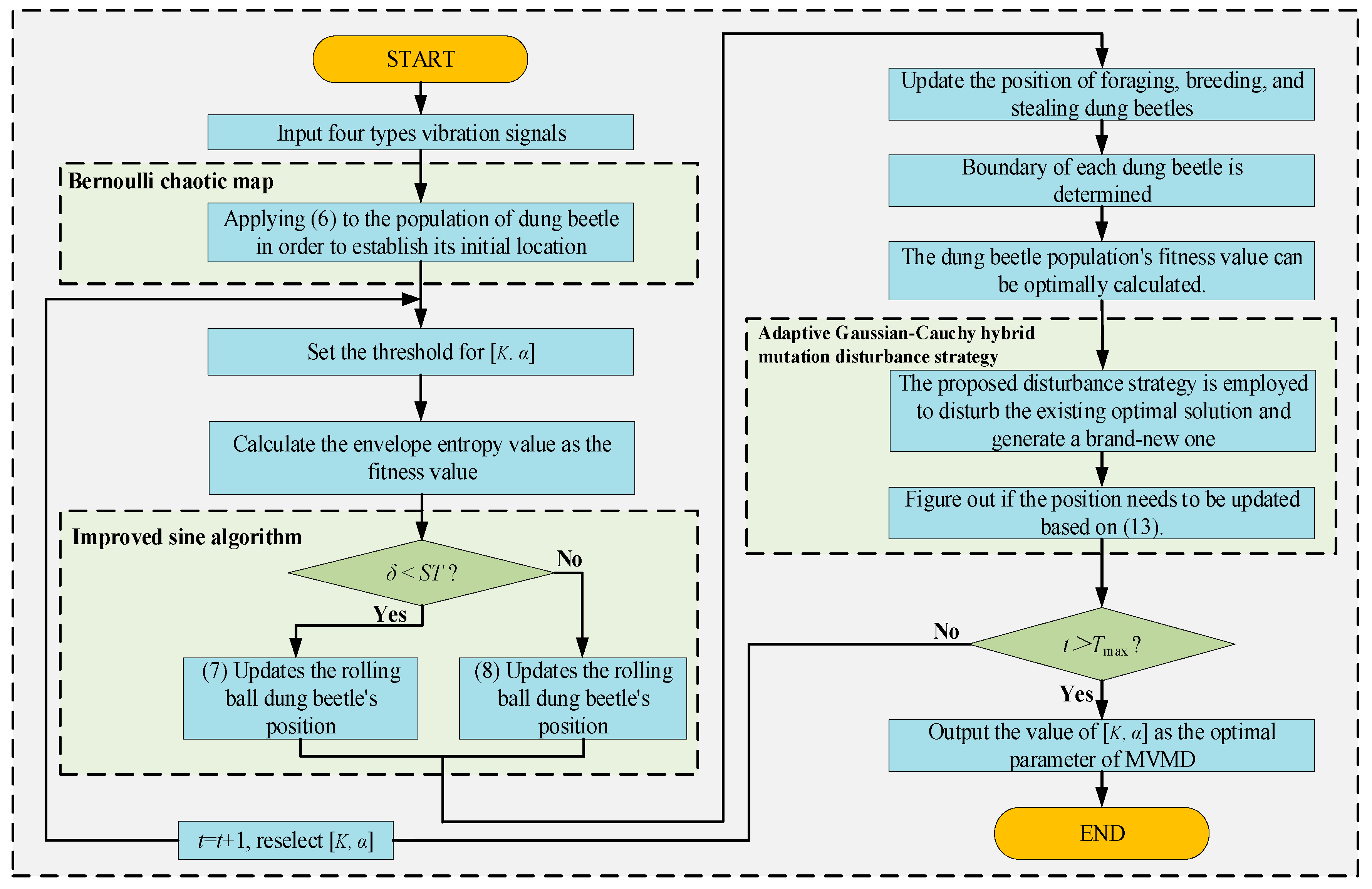
2.2. The Improved DBO Algorithm

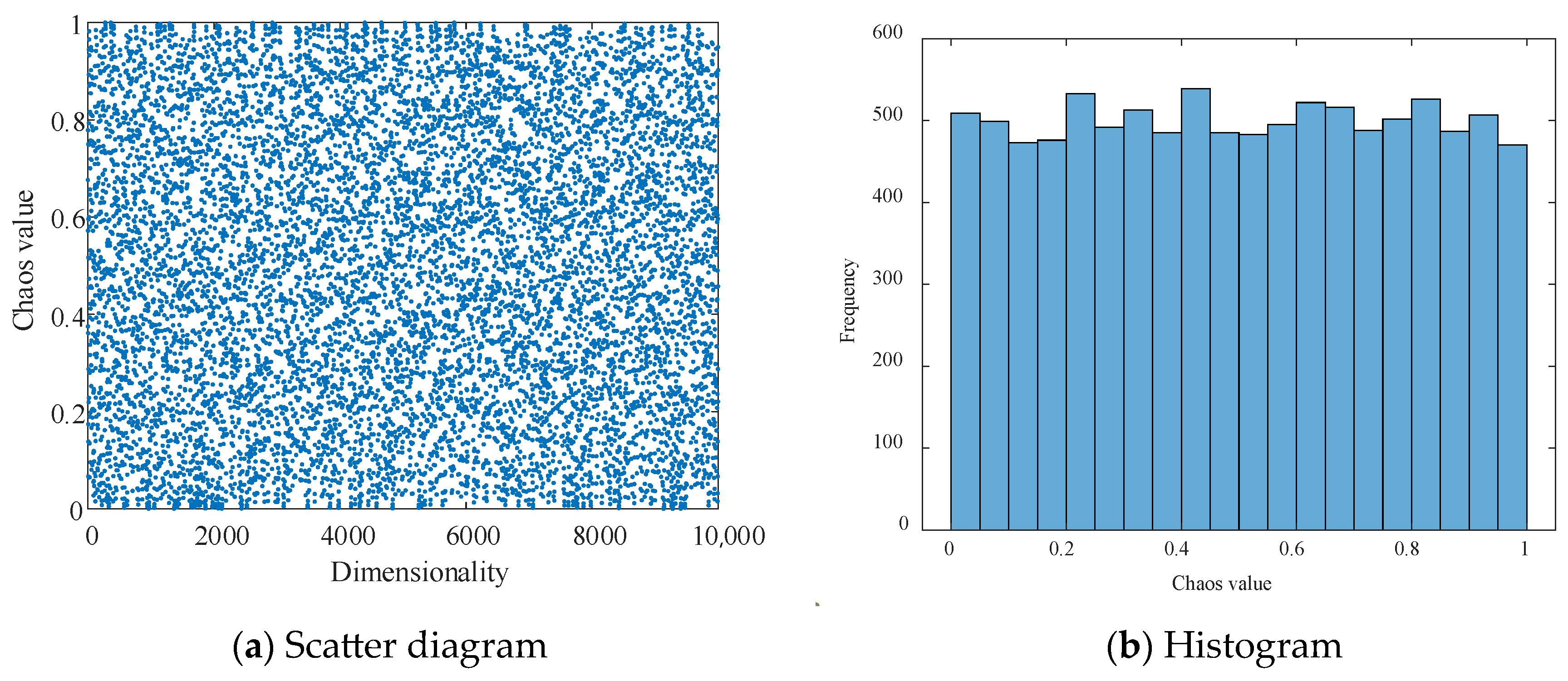
2.2.1. Bernoulli Chaotic Map Strategy

The population is initialized using the Bernoulli chaotic map to improve the diversity of the population. The distribution of the Bernoulli chaotic map from 0 to 1 is more uniform and its periodicity is more stable. The Bernoulli chaotic map is represented as
z n + 1 = z n 1 β ,   0 z n 1 β z n ( 1 β ) β ,   1 β z n 1
where the parameter β represents the map parameter and β ∈ (0,1). Here, we set β = 0.518 and z0 = 0.326, and the spatial dimension was set to 10,000 to achieve the best value. Figure 2 illustrates the sequence distribution of the Bernoulli chaotic map.

2.2.2. Improved Sine Algorithm (MSA)

During the process of dung beetles pushing the dung ball to the desired position, the direction is given and remains unchanged, and the position is updated synchronously, which can be expressed as follows:
x i ( t + 1 ) = x i ( t ) + a × k × x i ( t 1 ) + b × Δ x Δ x = x i ( t ) X w
where the parameter t signifies the current iteration count, and x i (t) signifies the position of the i-th dung beetle in the t-th iteration. The parameter a is designated as −1 or 1, signifying a natural coefficient; the parameter k belongs to the interval (0,0.2], signifying the deflection coefficient; the parameter b belongs to the interval (0,1), signifying a constant; Xw signifies the most unfavorable situation globally; and Δx signifies environmental changes.
In the process of the position iteration of dung beetles, the improved sine algorithm is used to iteratively optimize the position of dung beetle, and the sine function and adaptive variable inertia weight coefficient ωt are added, which allows for the simultaneous satisfaction of global exploration and local development. The following is an expression for the improved formula:
x i ( t + 1 ) = ω t x i ( t ) + r 1 × sin r 2 × r 3 p i ( t ) x i ( t )
where the parameter t represents the current iteration count, x i (t) represents the i-th component of the dung beetle position variable during the t-th iteration, p i (t) represents the i-th component of the optimal dung beetle position variable during the t-th iteration, r1 is a function that decreases nonlinearly, r2 is a random number generated between the interval [0,2π], and r3 is a random number generated between the interval [−2,2].
To determine the variation in r1 in the interval [0,π], the cosine function is employed:
r 1 = ω max ω min 2 cos π t T max + ω max + ω min 2
where ωmax and ωmin are the values that signify the maximum and minimum of ωt, respectively; t signifies the present iteration count; and Tmax signifies the maximum iteration count.
In addition, ωt decreases linearly with increasing t:
ω t = ω max ω max ω min × t T max
The position is updated using the sine guidance mechanism of MSA instead of the tangent strategy when the dung beetle travels. The improved formula is
x i ( t + 1 ) = x i ( t ) + a × k × x i ( t 1 ) + b × Δ x ,   δ   <   S T ω t x i ( t ) + r 1 × sin r 2 × r 3 p i ( t ) x i ( t ) ,   δ     S T
where the parameter δ represents a number generated at random between the interval [0,1), and the parameter ST belongs to the interval (0.5,1]. When δ is less than ST, the global exploration is normal, and (7) is called at this time. When δ is greater than or equal to ST, the search is carried out in a sine function, and (8) is called at this time [27].

2.2.3. Adaptive Gaussian–Cauchy Hybrid Mutation Disturbance Strategy

In the final phases of the iteration process, the DBO algorithm is prone to reaching a local optimum solution, which should be implemented to interact with individuals while simultaneously escaping from the local optimum solution. This study combines the advantages of Cauchy and Gaussian mutations and uses a hybrid mutation perturbation approach to disturb individuals. To simplify the method, only optimum individuals undergo mutational alterations, and a better position before and after the mutation is selected to enter the next iteration, which is expressed as follows:
H b ( t ) = X b ( t ) × 1 + μ 1 × Gauss ( σ ) + μ 2 × Cauchy ( σ )
where Xb(t) signifies the optimal location of individual X in the t-th iteration, Hb(t) signifies the location of Xb(t) after the Gaussian–Cauchy hybrid disturbance, Gauss(σ) signifies the operator for Gaussian mutations, Cauchy(σ) signifies the operator for Cauchy mutations, and μ1 = t/Tmax, μ2 = 1 − t/Tmax.
The greedy rule is used after the end of the variation perturbation update, and one method to assess whether the position will continue to be updated is to compare the fitness value of the previous position with that of the new position. The specific description is as follows:
X b = H b ( t ) , f H b ( t ) < f X b ( t ) X b ( t ) , f H b ( t ) f X b ( t )
where the fitness value corresponding to position x is denoted as f(x).

2.3. Improved Sine Algorithm–Dung Beetle Optimizer (MSADBO)

The MSADBO algorithm is compared with algorithms such as GWO, SSA, WOA, NGO, and DBO, and the F1–F4 functions of the CEC2005 function set were used for testing. Several algorithms were iterated 500 times, and the population size and dimensions were set to 30. Figure 3 displays the findings acquired after conducting the experiment 30 times, and it can be clearly seen that the MSADBO algorithm had a faster convergence speed and stronger optimization ability.
In this study, the MVMD parameters were optimized using MSADBO, and the minimum envelope entropy was selected as the fitness function. Compared with VMD, MVMD can increase the preset range of K values, which has greater advantages. The algorithm flow of MSADBO-MVMD is shown in Figure 4.

2.4. The Framework of Disconnector Mechanical Fault Diagnosis

This study introduces a mechanical fault diagnosis method for disconnectors based on parameter-optimized MVMD with an improved DBO and CNN-BiLSTM. Figure A1 in Appendix A shows the specific working structure and main steps of the method:
(1)
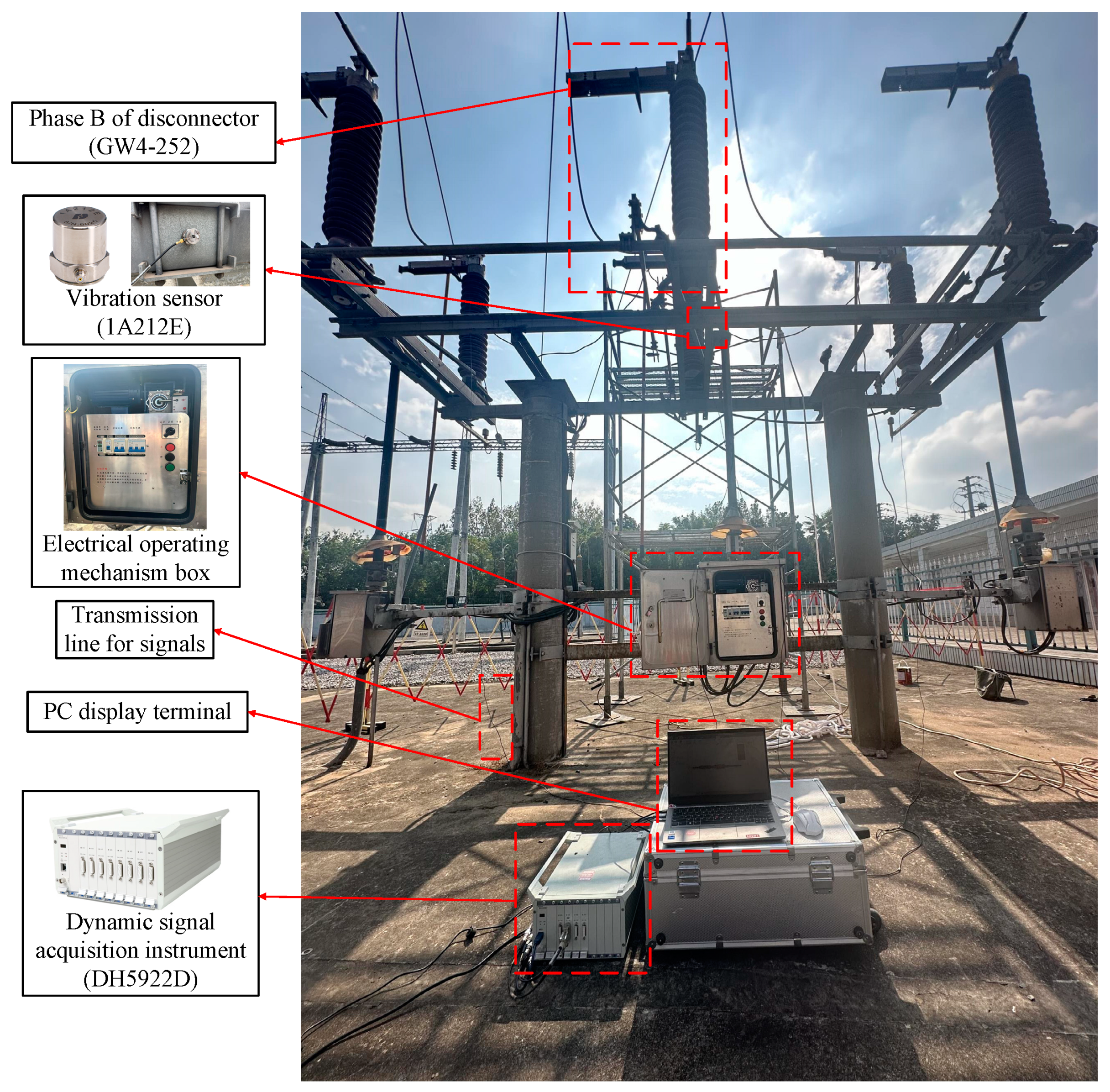
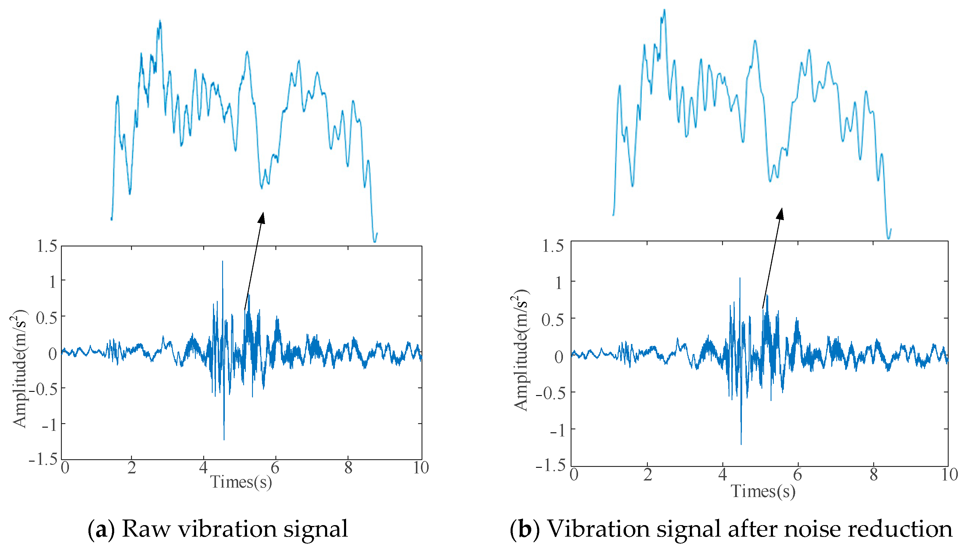
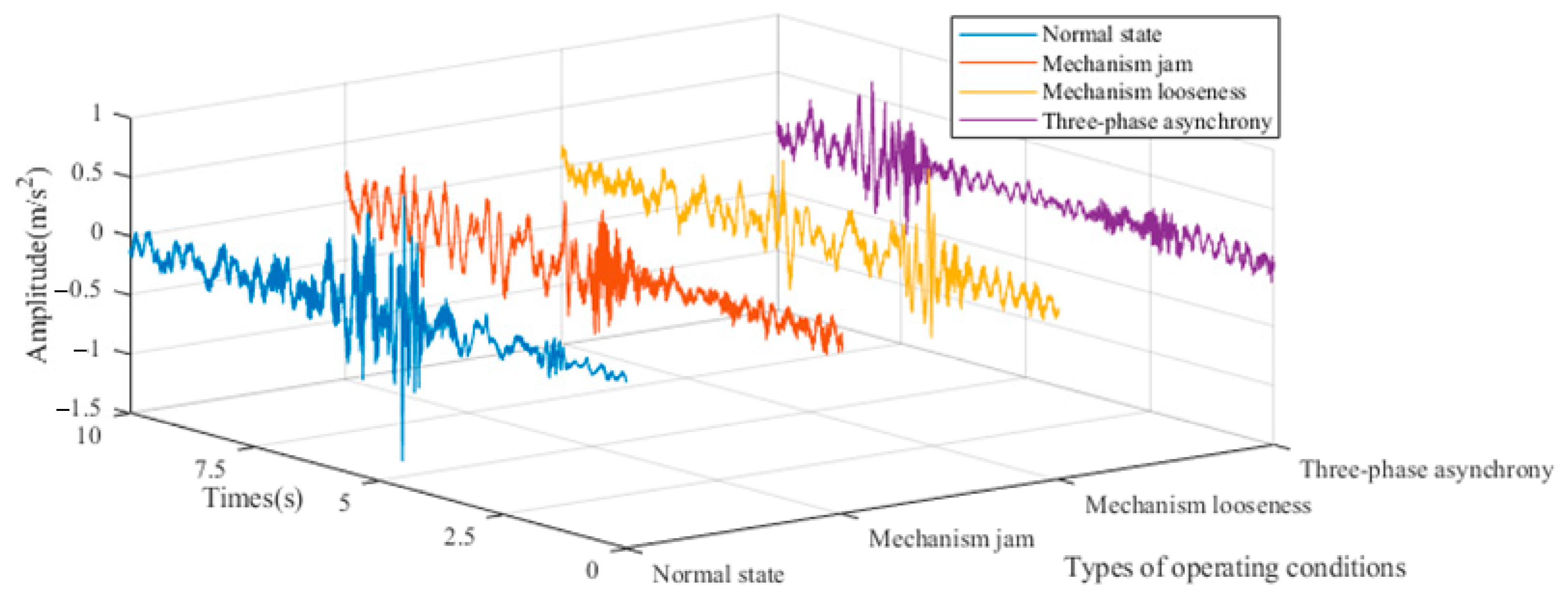
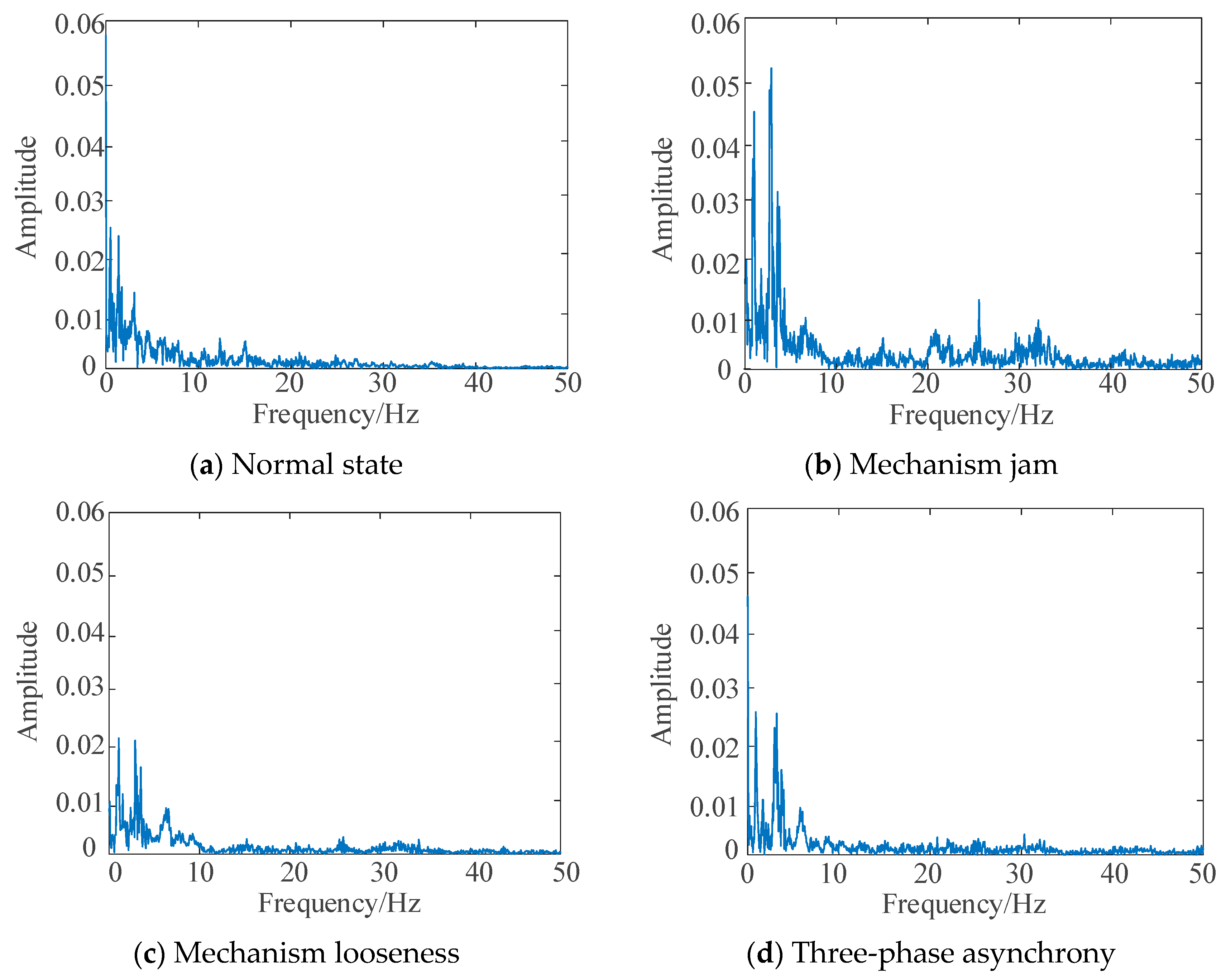
Vibration signal acquisition: Use the dynamic signal acquisition instrument to extract vibration signals including normal state, mechanism jam, mechanism looseness, and three-phase asynchrony, and display and store using the host computer software (Dong-Hua Test: Real Time Data Measurement and Analysis Software System).
(2)
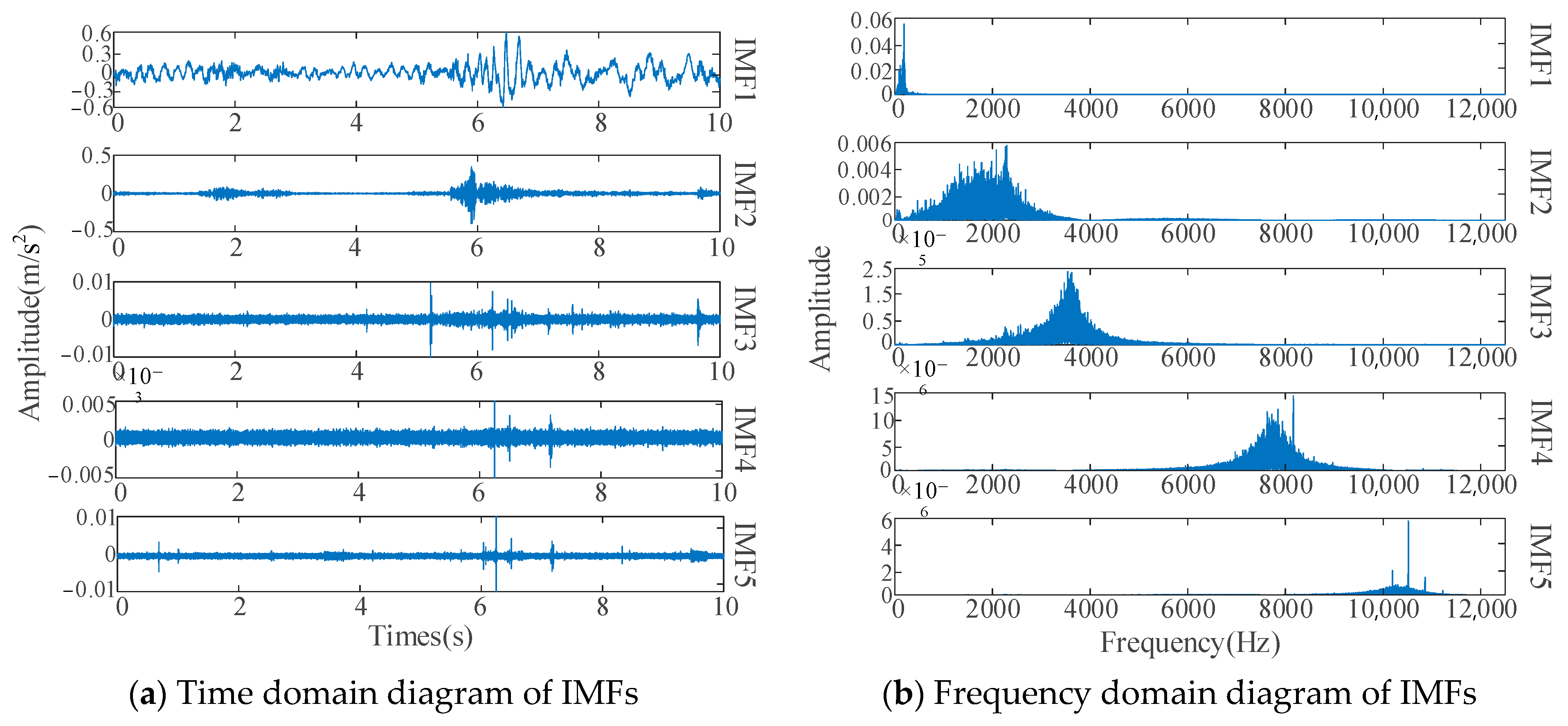
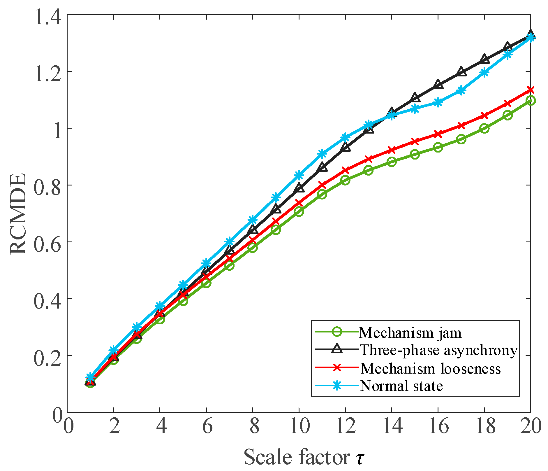
Feature selection and extraction: MSADBO is utilized for the optimization of parameters K and α in MVMD. After selecting the optimal parameters, MVMD is used to decompose the signals of different fault types to obtain the IMF components. Calculate the Pearson correlation coefficient between each IMF component and the raw signal and select IMF components whose coefficient value is greater than 0.1 to retain. The energy value, refined composite multiscale diversity entropy (RCMDE), and 13 time–frequency domain eigenvalues are extracted from the energy, entropy, and time–frequency features to form a 34-dimensional initial feature matrix. Afterwards, the 34-dimensional initial feature matrix is reduced to a two-dimensional matrix by the t-SNE algorithm.
(3)
Fault classification: Based on a ratio of 3:1, the dataset is partitioned into training and test sets. Fault identification is performed using CNN-BiLSTM and then assessed using the test set. The results of the disconnector mechanical fault diagnosis are output.

3. Disconnector Fault Experiment

3.1. Experimental Platform

In this study, a GW4-252 type outdoor high voltage disconnector in a 220 kV substation was taken as the test object, and the fault diagnosis test scheme of the disconnector was designed. Figure 5 shows the experimental platform for the outdoor disconnector vibration established in this study. The experimental platform simulated three typical mechanical faults of the disconnector and collect the vibration signals. The experimental platform included a disconnector, a dynamic signal acquisition device, four vibration sensors, an electrical operating mechanism box, a PC display terminal, and several transmission lines for the signal.
There are many types of vibration sensors, according to the different physical quantities measured, and they are mainly divided into displacement sensors, velocity sensors, acceleration sensors, etc. In this study, the 1A212E piezoelectric acceleration sensor, which is more sensitive to mechanical vibration and has a wider frequency range, was selected. It has the characteristics of light weight, high sensitivity, large measurement range, and simple installation. The weight was 65 g, the sensitivity was 50 mV/m·s−2, and the measurement range was −10 g ± 10 g. The selected 1A212E piezoelectric acceleration sensor was connected to the four measuring points of the disconnector through a planar magnetic seat.
The selected DH5922D dynamic signal acquisition equipment has strong anti-interference ability and good stability. It can record multi-channel signals in real time for a long time without interruption. All channels work synchronously in parallel during the acquisition period, and the maximum sampling rate is 256 kHz/channel. The system has a built-in 24 V/4 mA bias circuit to collect the output signal of the piezoelectric acceleration sensor and realize the test and analysis of the vibration signal.

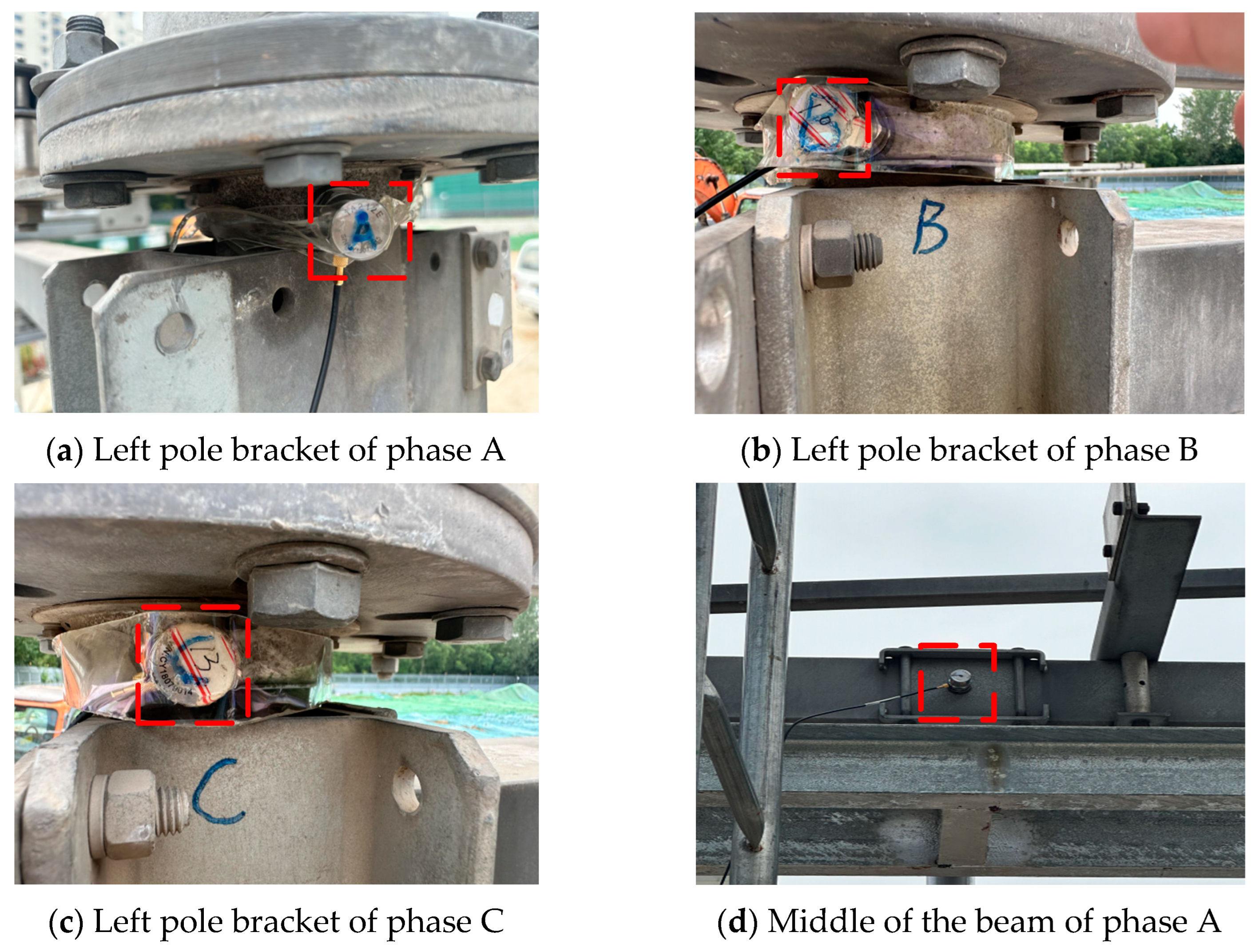
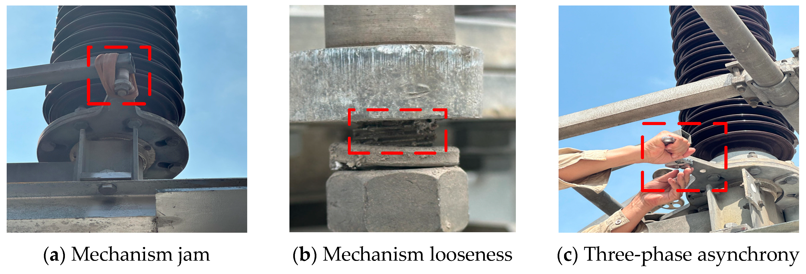
3.2. Sensor Arrangement and Fault Setting

The installation positions of the vibration sensors are illustrated in Figure 6. After evaluating the vibration intensity and acquisition effect and communicating with on-site technicians, the measurement point in the middle of the beam of phase A was selected for signal analysis.
Figure 7 illustrates the fault-setting process. In Figure 7a, multiple rubber elastic ropes were tied to the junction components of the transmission mechanism to simulate the mechanism jam failure. In Figure 7b, the joint bolts of the active pole connecting rod of phase A were loosened to achieve the effect of the mechanism looseness failure. In Figure 7c, the driven pole arm of phase A was adjusted to make phase A lag behind phases B and C to simulate the three-phase asynchrony failure.

3.3. Experimental Process

The sampling frequency of the vibration signal in this experiment was set to 5 kHz, and 120 groups were tested in each state to increase the number of samples. After starting the detection, the electric closing operation of the disconnector was performed, the closing button in the electric operating mechanism box was pressed, and the detection was stopped after closing; the closing process time was 10 s. Because the data acquisition in this experiment was disturbed by surrounding noise, the wavelet packet noise reduction algorithm was used to denoise the collected data. The particular steps involved in the algorithm are illustrated in [28], and the noise reduction process is illustrated by considering the normal state as an example, as shown in Figure 8. The vibration signals after noise reduction under the four operating conditions are shown in Figure 9.
It can be seen from Figure 9 that the measured vibration signals of the disconnector under four operating conditions were different in the time domain, but the time domain diagram can only obtain its qualitative difference, it was difficult to identify the signal characteristics by the naked eye, and the MVMD algorithm needed to set the parameter K in advance when decomposing the signal. Therefore, the main frequency distribution of the vibration signal under four operating conditions was obtained by Fourier transform, and the results are shown in Figure 10.
From spectrum diagrams, it can be seen that the frequency range of the collected signal was basically less than 50 Hz when the disconnector was closed. The frequency component of the vibration signal of the disconnector was complex, and the non-stationarity was strong. Therefore, the time–frequency energy analysis method was used to analyze the measured vibration signal, and the time–frequency energies of the vibration signal of the disconnector under four different operating conditions were obtained. The wavelet packet transform algorithm was introduced here, and taking the three-layer wavelet transform as an example, the sampling frequency was 200 Hz, while according to the Nyquist theory, the measured signal frequency was less than 100 Hz. After decomposition, the components of eight equal frequency bands in the range of 0~100 Hz were obtained. The time–frequency energy values under four operating conditions were calculated, as shown in Figure 11.
From Figure 11, it can be seen that the energy was concentrated within 50 Hz under four operating conditions. In general, the energy value was the highest under mechanism jam. The reason was that the output power of the motor became larger, and the vibration frequency of the equipment became larger when the jam fault occurred, which led to the increase in the energy value. The energy value was the lowest under mechanism looseness. The reason was that the gap of the transmission mechanism became larger and the vibration frequency of the equipment became lower when the loose fault occurred, which led to the decrease in the energy value.
When the disconnector fails, the fundamental frequency component and the frequency doubling component will change, showing different degrees of suppression and enhancement effects. Therefore, selecting the appropriate parameter K for the MVMD algorithm is helpful to better identify the fault type of the disconnector. At this time, compared with other algorithms, the improved DBO algorithm was used to optimize the MVMD, which can obtain the best parameters more accurately and improve the efficiency of fault diagnosis.

4. Result Analysis

4.1. Vibration Signal Decomposition Based on MSADBO-MVMD

The MSADBO-MVMD decomposition was performed on each group of signals under the four operating conditions, and the parameter settings are presented in Table 1.
The MSADBO-MVMD algorithm was loaded, and the values of K and α for each group of data at the minimum envelope entropy were recorded. Table 2 shows the optimization results of the MSADBO-MVMD parameters under the four operating conditions.
The optimization results were initialized as MVMD parameters, and MVMD decomposition was performed. Taking the vibration signal under the three-phase asynchrony as an example, Figure 12 illustrates the results of the MVMD decomposition.
It can be seen from Figure 12b that the center frequency of IMFs increased from low frequency to high frequency under three-phase asynchrony, and there was only one obvious main frequency in the spectrum of each IMF. All five IMFs were effectively separated without modal aliasing. In addition, the information features contained in the waveforms of all IMFs were basically consistent with the original vibration signals, but the complexity was significantly reduced, being simpler and more intuitive. This also highlights that MVMD has more advantages in processing multivariate data than signal decomposition algorithms such as VMD and EMD.

4.2. Feature Extraction

4.2.1. Selection of IMFS

To obtain effective IMFs, we first determined the Pearson correlation coefficients of the raw signal-to-IMFs, and then we selected the threshold d. The IMF was chosen as the effective component if the value of the correlation coefficient was larger than d; otherwise, it was abandoned. After several trials, d was adjusted to 0.1 in an effort to obtain the maximum number of IMF components. Taking the mechanism jam as an example, the correlation coefficient value was obtained, as shown in Figure 13. The correlation coefficient values for the four operating conditions are listed in Table 3.
Table 3 indicates that IMF1-IMF3 were selected as effective components for mechanism jam and mechanism looseness, and IMF1-IMF2 were selected as effective components for normal state and three-phase asynchrony.

4.2.2. Construction of Fusion Feature Matrix

(1)
Energy feature extraction
A wealth of fault information was included in the energy that corresponded to the IMF component of the disconnector vibration signal. This information can be used to extract the features of the fault fully. The following steps are required to obtain the energy value:
Step 1: Total energy value of the k IMFs after each signal decomposition is calculated as Ei = |c(t)|2dt, where c(t) is the amplitude of the IMF at time t, i = 1, ···, k.
Step 2: Calculate the sum of squares of each signal energy: E = ( i = 1 k |Ei|2)1/2.
Step 3: After the normalization of k IMFs, the energy characteristic matrix is obtained: Ti = [E1/E, ···, Ek/E].
Step 4: For each operating condition, each useful IMF is used to average the energy value, and the energy matrix E = [ T 1 ¯ ;   T 2 ¯ ;   T 3 ¯ ;   T 4 ¯ ] under four groups of vibration signal data (four operating conditions) is obtained, where T 1 ¯ ~ T 2 ¯ is the energy value after averaging the effective IMF under each operating condition.
(2)
Entropy feature extraction
The RCMDE was proposed by integrating the benefits of MDE with a composite coarse-grained time series [29,30]. The RCMDE generates multiple time series at multiple scales through a sliding process and uses multiple time series to estimate, which can more accurately calculate the state probability in the phase space and improve the stability of the MDE at high scales.
The RCMDE value for each IMF is calculated after selecting effective IMF components for each operating condition. At this time, scaling factor τ, embedding dimension m and symbol interval number ε, must be set. Typically, τ > 10, where the maximum scale factor of the sequence is set to τmax = 20. For the embedded dimension m, if m is too small, a large amount of information on faults will be lost; if m is excessively large, the computational efficiency of entropy will be reduced. Therefore, in this study, m = 4. Based on the results of previous studies, we set ε = 30. The delay time t has little effect on the entropy calculation and is generally set to t = 1.
The RCMDE values of the effective IMF components under four operating conditions were calculated. For each operating condition, the CMWPE values were averaged using each effective IMF component, and the results are shown in Figure 14.
Figure 14 illustrates that under varying operating conditions, the overall trend of the vibration signals had different fluctuations at different scales, which also indicates that the use of RCMDE as a feature vector can effectively distinguish various operating conditions. The entropy characteristic matrix for the four groups of vibration signals is obtained as follows:
R = R C M D E 1 , 1 R C M D E 1 , 20 R C M D E 4 , 1 R C M D E 4 , 20
(3)
Time–frequency feature extraction
As the most basic method of signal feature extraction, the time–frequency domain method can analyze fault features more accurately and clearly. Therefore, for each effective IMF component, 10 time–domain characteristic parameters were extracted; among them, there were five dimensional parameters, which were maximum value t1, peak-to-peak value t2, variance t3, standard deviation t4, and root mean square t5, and there were five dimensionless parameters, which were crest factor t6, pulse factor t7, margin factor t8, kurtosis factor t9, and waveform factor t10. Three frequency domain characteristic parameters were extracted, which were center of gravity frequency p1, mean square frequency p2, and frequency variance p3.
For a set of vibration signal data, the feature matrices were as follows: t = [t1, t2, ···, t10] for the time domain, p = [p1, p2, p3] for the frequency domain, and B = [t, p] = [t1, t2, ···, t10, p1, p2, p3] for the time–frequency domain obtained after splicing. The calculation formula for the selected parameters is listed in Table 4, where x(n) represents the input signal, and its corresponding spectrum was s(k), k = 1, ···, K, where K signifies the total number of spectral lines in the spectrogram, and f(k) signifies the frequency value of the k-th spectral line.

4.2.3. Dimensionality Reduction of Fusion Feature Matrix

In summary, the fusion feature matrix Q = [E, R, B] is established based on the energy, entropy, and time–frequency features. The fusion feature matrix can comprehensively reflect fault information and provide a more comprehensive basis for subsequent fault classification. A 480 × 34 feature matrix was generated for each disconnector operating condition (each containing 120 samples). Because the feature matrix had an excessively large dimension, the subsequent fault classification process was slow. Therefore, the t-SNE method was employed to decrease the dimensions before entering the classifier [31]. t-SNE is a nonlinear dimensionality reduction technique, which is especially suitable for the visualization of high-dimensional data. It is derived from the SNE algorithm and uses the t distribution in the low-dimensional space, which effectively solves the problem of data point congestion in the SNE algorithm. The core idea is to map high-dimensional data to low-dimensional space (two-dimensional or three-dimensional) by preserving the local structure of the data.
In this study, the t-SNE algorithm was used to reduce the high-dimensional feature matrix to a two-dimensional matrix. The two-dimensional plane can be clearly presented without complex interaction. While retaining the main structure, it can effectively suppress the random fluctuations in the high-dimensional space. Although the three-dimensional matrix may retain more information, it may introduce redundant information and increase the difficulty of observation. Figure 15 illustrates the results of the dimensionality reduction, which shows that the discrimination between different types of data was significantly increased, but at the same time, there was still a mixture of different fault samples. Therefore, it is necessary to further apply the classification model for fault classification.

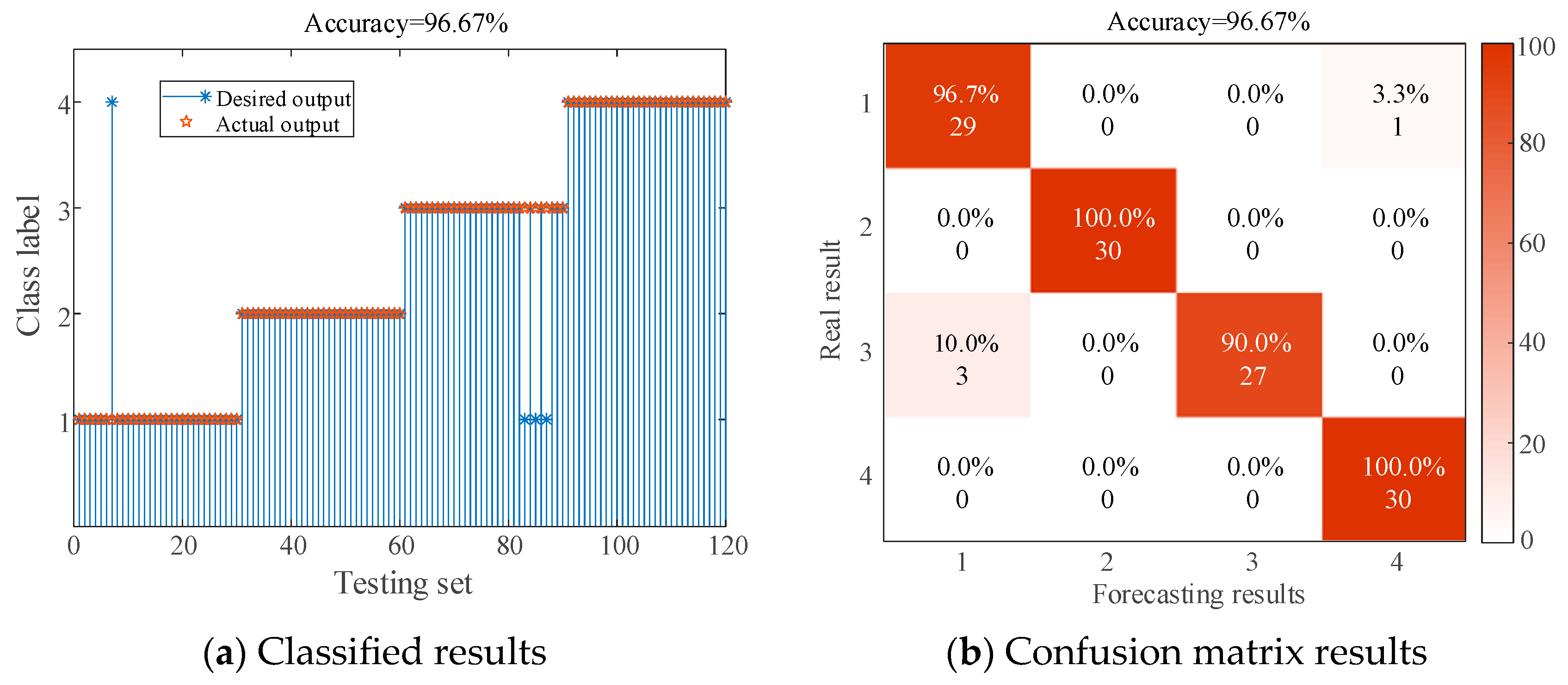
4.2.4. Fault Identification

We used the CNN BiLSTM as the fault classifier. The BiLSTM layer was inserted between the pooling layer and the fully connected layer; taking into account the forward and backward information of the feature data, the model can efficiently learn the deep features and dynamic information of the feature vectors, adaptively capture the fault features under different operating conditions, and improve the classification accuracy. The parameter settings are shown in Table 5. In addition, the network training algorithm was ‘adam’, the learning rate was set to 0.001, and the number of iterations was set to 300.
Based on the ratio of 3:1, the feature data set after dimensionality reduction was partitioned into training and test sets, and we obtained a 360 × 2 training set and a 120 × 2 test set. At the same time, each type of operating condition was labeled, and 1–4 represent normal state, mechanism jam, mechanism looseness, and three-phase asynchrony, respectively. The results for the test set are shown in Figure 16.
Figure 16 shows that the proposed model was erred by mistaking a group of normal state as three-phase asynchrony, three groups of mechanism looseness were mistaken for normal state, and the overall identification accuracy reached 96.67%. The effectiveness and superiority of this method were verified by a comparison with other relevant methods, as presented in Table 6.
Compared with #1 and #2, MVMD had a better decomposition effect than VMD. From #1, #3, and #4, the identification accuracy of the DBO algorithm was significantly improved after optimization and had a higher accuracy than that of the other algorithms. From #1, #5, #6, and #7, the addition of the BiLSTM layer captured the fault characteristic information more comprehensively and had a higher accuracy than the other classifiers. From #1, #8, #9, and #10, it can be seen that extracting fault features from multiple dimensions can better identify faults. Compared with #1 and #11, the t-SNE algorithm had a better dimensionality reduction effect than the PCA algorithm, which improved recognition accuracy.

5. Conclusions

This study introduced a novel approach for the diagnosis of mechanical faults in disconnectors. Three solutions were proposed to enhance the performance of DBO by addressing its deficiencies. MSADBO-MVMD was employed for the purpose of decomposing the vibration signal and adaptively determining the optimum K and α. The effective IMFs were determined using the Pearson correlation coefficient method, and their fusion eigenvalues were calculated to construct the eigenvector matrix. The t-SNE algorithm was introduced, and the dimension was reduced to the final eigenvector. The CNN-BiLSTM model was utilized for fault identification. Based on the disconnector fault experimental platform, three typical mechanical faults were simulated. After comparing a large number of research results, the conclusions are as follows:
(1)
By introducing the MSADBO, significant progress has been made in addressing the issues of slow convergence speed and the tendency to easily slip into the local optimum of the DBO. The parameters K and α of the MVMD can be optimally selected to adaptively decompose the vibration signal.
(2)
Selecting effective IMFs based on Pearson correlation coefficient and extracting features from energy, entropy, and time–frequency domains can fully mine potential fault features and improve the accuracy of fault diagnosis.
(3)
The dimensions of the feature matrix can be minimized utilizing the t-SNE method, and CNN-BiLSTM is used for fault identification, which significantly reduces the time required for operation and improves the performance of the algorithm model.
(4)
Three kinds of disconnector mechanical fault setting methods and the best arrangement of sensors are proposed. The vibration data under four operating conditions are collected to diagnose the mechanical fault of the disconnectors. To a certain extent, the problem of insufficient sample size of disconnectors fault data is solved.
In addition, the model proposed in this paper has good recognition accuracy and generalization ability for fault diagnosis of disconnector, but its applicability to other equipment remains to be studied. In the future, the applicability of the model will be strengthened, and the type of fault diagnosis equipment will be expanded.

Author Contributions

Conceptualization, C.Z. and H.M.; methodology, C.Z. and H.M.; formal analysis, C.Z.; investigation, C.Z. and W.S.; data curation, C.Z.; writing—original draft preparation, C.Z.; writing—review and editing, C.Z., H.M. and W.S. All authors have read and agreed to the published version of the manuscript.

Funding

This research was funded by the National Natural Science Foundation of China, grant number 51577050 (Hongzhong Ma); in part by the Natural Science Foundation of Jiangsu Province, China, grant number BK20231460 (Baowen Liu); and in part by the Science and Technology Project of State Grid Jiangsu Electric Power Corporation, grant number J2024047 (Hongzhong Ma).

Data Availability Statement

Data are contained within the article.

Conflicts of Interest

The authors declare no conflicts of interest.

Appendix A

Figure A1. Working structure of the proposed method.
Machines 13 00332 g0a1

References

  1. Lin, S.; Zhang, K.; Wang, Q. Fault diagnosis method of disconnector based on operating torque in closing process. In Proceedings of the 2021 IEEE 2nd China International Youth Conference on Electrical Engineering, Chengdu, China, 15–17 December 2021; pp. 1–6. [Google Scholar]
  2. Jürgensen, J.H.; Brodersson, A.L.; Nordström, L.; Hilber, P. Impact assessment of remote control and preventive maintenance on the failure rate of a disconnector population. IEEE Trans. Power Del. 2018, 33, 1501–1509. [Google Scholar] [CrossRef]
  3. Mardegan, C.S.; Shipp, D.D. Anatomy of a complex electrical failure and its forensics analysis. IEEE Trans. Ind. Appl. 2014, 50, 2910–2918. [Google Scholar] [CrossRef]
  4. Cao, S.; Zhao, T.; Wang, G.; Zhang, T.; Liu, C.; Liu, Q.; Zhang, Z.; Wang, X. A Mechanical Defect Localization and Identification Method for High-Voltage Circuit Breakers Based on the Segmentation of Vibration Signals and Extraction of Chaotic Features. Sensors 2023, 23, 7201. [Google Scholar] [CrossRef] [PubMed]
  5. Runde, M. Failure frequencies for high-voltage circuit breakers, disconnectors, earthing switches, instrument transformers, and gas-insulated switchgear. IEEE Trans. Power Del. 2013, 28, 529–530. [Google Scholar] [CrossRef]
  6. Peng, T.; Lv, C.; Du, Y.; Lin, F.; Dong, S. Mechanical fault diagnosis of high voltage disconnector based on motor current detection. In Proceedings of the 2019 IEEE 3rd Information Technology, Networking, Electronic and Automation Control Conference, Chengdu, China, 15–17 March 2019; pp. 1726–1729. [Google Scholar]
  7. Liu, Q.; Wang, X.; Guo, Z.; Li, J.; Xu, W.; Dai, X.; Liu, C.; Zhao, T. Research on Circuit Breaker Operating Mechanism Fault Diagnosis Method Combining Global-Local Feature Extraction and KELM. Sensors 2024, 24, 124. [Google Scholar] [CrossRef] [PubMed]
  8. Souza, M.D.; Dhara, R.S.; Bouyer, R.C. Modularization of high voltage gas insulated substations. IEEE Trans. Ind. Appl. 2020, 56, 4662–4669. [Google Scholar] [CrossRef]
  9. Huang, S.; Shang, B.; Song, Y.; Zhang, N.; Wang, S.; Ning, S. Research on real-time disconnector state evaluation method based on multi-source images. IEEE. Trans. Instrum. Meas. 2022, 71, 1–15. [Google Scholar] [CrossRef]
  10. Yan, P.; Chang, C.; Hua, D.; Huang, H.; Liu, S.; Cui, P. Adaptive Disconnector States Diagnosis Method Based on Adjusted Relative Position Matrix and Convolutional Neural Networks. Sensors 2025, 25, 1701. [Google Scholar] [CrossRef]
  11. Qiu, Z.; Ruan, J.; Huang, D.; Huang, Y. Mechanical fault diagnosis of high voltage outdoor disconnector based on motor current signal analysis. In Proceedings of the 2014 International Conference on Power System Technology, Chengdu, China, 20–22 October 2014; pp. 1193–1198. [Google Scholar]
  12. Zhang, J.; Xu, H.; Wang, X.; Ding, Y.; Dai, X.; Hao, J. Mechanical defect field detection for operational GIS equipment based on vibration signal analysis. In Proceedings of the 2021 6th Asia Conference on Power and Electrical Engineering, Chongqing, China, 8–11 April 2021; pp. 1244–1248. [Google Scholar]
  13. Sun, S.; Zhang, T.; Li, Q.; Wang, J.; Zhang, W.; Wen, Z.; Tang, Y. Fault diagnosis of conventional circuit breaker contact system based on time-frequency analysis and improved AlexNet. IEEE. Trans. Instrum. Meas. 2021, 70, 1–12. [Google Scholar] [CrossRef]
  14. Fu, Q.; Jing, B.; He, P.; Si, S.; Wang, Y. Fault feature selection and diagnosis of rolling bearings based on EEMD and optimized elman_adaBoost algorithm. IEEE Sens. J. 2018, 18, 5024–5034. [Google Scholar] [CrossRef]
  15. Geraei, H.; Rodriguez, E.A.V.; Majma, E.; Habibi, S.; Al-Ani, D. A Noise Invariant Method for Bearing Fault Detection and Diagnosis Using Adapted Local Binary Pattern (ALBP) and Short-Time Fourier Transform (STFT). IEEE Access. 2024, 12, 107247–107260. [Google Scholar] [CrossRef]
  16. Sun, W.; Ma, H.; Wang, S. A novel fault diagnosis of GIS partial discharge based on improved whale optimization algorithm. IEEE Access. 2024, 12, 3315–3327. [Google Scholar] [CrossRef]
  17. Song, Q.; Jiang, X.; Wang, S.; Guo, J.; Huang, W.; Zhu, Z. Self-adaptive multivariate variational mode decomposition and its application for bearing fault diagnosis. IEEE. Trans. Instrum. Meas. 2022, 71, 1–13. [Google Scholar] [CrossRef]
  18. Xue, J.; Shen, B. Dung beetle optimizer: A new meta-heuristic algorithm for global optimization. J. Supercomput. 2023, 79, 7305–7336. [Google Scholar] [CrossRef]
  19. Chang, B.; Zhao, X.; Guo, D.; Zhao, S.; Fei, J. Rolling bearing fault diagnosis based on optimized VMD and SSAE. IEEE Access. 2024, 12, 130746–130762. [Google Scholar] [CrossRef]
  20. Zhang, C.; Wang, C.; Zhang, D.; Li, L.; Yang, S. Improved probabilistic neural network based fault diagnosis of control valve. In Proceedings of the 2023 CAA Symposium on Fault Detection, Supervision and Safety for Technical Processes, Yibin, China, 22–24 September 2023; pp. 1–6. [Google Scholar]
  21. Zhang, L.; Fu, Z. Harmonic research on fault reconfiguration of active distribution network based on multi-strategy fusion and improved dung beetle optimization algorithm. In Proceedings of the 2024 6th International Conference on Energy Systems and Electrical Power, Wuhan, China, 21–23 June 2024; pp. 843–846. [Google Scholar]
  22. Yang, C.; Wu, X.; Gong, W.; Wang, Q.; Li, L. An intelligent identification algorithm for obtaining the state of power equipment in SIFT-based environments. Int. J. Performability Eng. 2019, 15, 2382–2391. [Google Scholar]
  23. Wang, Q.; Zhang, K.; Lin, S. Fault diagnosis method of disconnector based on CNN and D-S evidence theory. IEEE Trans. Ind. Appl. 2023, 59, 5691–5704. [Google Scholar] [CrossRef]
  24. Sun, M.; Bai, X.; Zhang, W.; Ye, L. Jointed task of multi-scale CNN based power transformer fault diagnosis with vibration and sound signals. In Proceedings of the 2023 Panda Forum on Power and Energy, Chengdu, China, 27–30 April 2023; pp. 1761–1765. [Google Scholar]
  25. Wang, W.; Zhang, D.; Hu, X.; Han, R.; Guo, Y.; Qiao, Y.; Gao, S.; Wang, Z. Recognition of Complex Abnormal Vibration Voiceprint of Power Transmission and Transformation Equipment in Cold Environment. In Proceedings of the 2024 IEEE 7th Eurasian Conference on Educational Innovation, Bangkok, Thailand, 26–28 January 2024; pp. 394–398. [Google Scholar]
  26. Ma, W.; Liu, S.; Liang, H.; Zhang, S.; Gao, Y.; Li, D.; Di, X. Fault diagnosis of integrated energy system based on CNN-LSTM. In Proceedings of the 2023 42nd Chinese Control Conference, Tianjin, China, 24–26 July 2023; pp. 5102–5107. [Google Scholar]
  27. Ma, W.; Ren, X.; Chen, Z. A new signal analysis method after wavelet packet de-noising. In Proceedings of the 2008 International Conference on Wavelet Analysis and Pattern Recognition, Hong Kong, China, 30–31 August 2008; pp. 426–431. [Google Scholar]
  28. Pan, J.; Li, S.; Zhou, P.; Yang, G.; Lv, D. Dung beetle optimization algorithm guided by improved sine algorithm. Comput. Eng. Appl. 2023, 59, 92–110. [Google Scholar]
  29. Zhao, S.; Chen, Y.; Rehman, A.U.; Liang, F.; Wang, S.; Zhao, Y.; Deng, W.; Ma, Y.; Cheng, Y. Detection of interturn short-circuit faults in DFIGs based on external leakage flux sensing and the VMD-RCMDE analytical method. IEEE. Trans. Instrum. Meas. 2022, 71, 1–12. [Google Scholar] [CrossRef]
  30. Dhandapani, R.; Mitiche, I.; McMeekin, S.; Morison, G. A novel bearing faults detection method using generalized Gaussian distribution refined composite multiscale dispersion entropy. IEEE. Trans. Instrum. Meas. 2022, 71, 1–12. [Google Scholar] [CrossRef]
  31. Zhai, H.; Wang, X.; Ge, M.; Feng, S.; Cheng, L.; Deng, Y. Improved fault classification method in transmission line based on K-means clustering. In Proceedings of the 2020 5th Asia Conference on Power and Electrical Engineering, Chengdu, China, 4–7 June 2020; pp. 154–158. [Google Scholar]
Figure 1. Model structure of CNN-BiLSTM.
Machines 13 00332 g001
Figure 2. Sequence distribution of the Bernoulli chaotic map.
Machines 13 00332 g002
Figure 3. Results of test functions.
Machines 13 00332 g003
Figure 4. Algorithm flow chart of the MSADBO-MVMD.
Machines 13 00332 g004
Figure 5. Vibration experimental platform of disconnector.
Machines 13 00332 g005
Figure 6. Installation position of vibration sensors.
Machines 13 00332 g006
Figure 7. Fault simulation methods of three typical mechanical faults.
Machines 13 00332 g007
Figure 8. Comparison of noise reduction effects under normal state.
Machines 13 00332 g008
Figure 9. Vibration signal after noise reduction under four operating conditions.
Machines 13 00332 g009
Figure 10. Spectrum diagrams of vibration signals under four operating conditions.
Machines 13 00332 g010
Figure 11. The time–frequency energy values of vibration signals under four operating conditions.
Machines 13 00332 g011aMachines 13 00332 g011b
Figure 12. Decomposition results of MSADBO-MVMD.
Machines 13 00332 g012
Figure 13. Pearson correlation coefficients of IMFs.
Machines 13 00332 g013
Figure 14. RCMDE values of effective IMFs under four operating conditions.
Machines 13 00332 g014
Figure 15. Results of t-SNE dimensionality reduction.
Machines 13 00332 g015
Figure 16. Results of the test set.
Machines 13 00332 g016
Table 1. Parameter settings of MSADBO-MVMD.
Population SizeMaximum Number of IterationsInitial Setting Value of (K, α)Value Range of KValue Range of α
2030(5,2000)(1,100)(10,3000)
Table 2. Parameter optimization results of MSADBO-MVMD.
Type of Operating ConditionsKαf
Normal state63756.7197
Mechanism jam72687.4136
Mechanism looseness812457.8438
Three-phase asynchrony516156.7453
Table 3. Pearson correlation coefficient values of IMFs under four operating conditions.
Pearson Correlation CoefficientNormal StateMechanism JamMechanism LoosenessThree-Phase Asynchrony
d10.96000.94000.98000.9600
d20.33000.21000.32000.3400
d30.03200.37000.12000.0250
d40.00670.08700.02400.0099
d50.00590.00610.00530.0061
d60.00510.00340.0064-
d7-0.00270.0060-
d8--0.0041-
Table 4. Formulas of characteristic parameters in the time-frequency domain.
Time Domain (Dimensional)Time Domain (Dimensionless)Frequency Domain
t1 t 1 = max ( x ( i ) ) t6 t 6 = max ( x ( i ) ) t 5 p1 p 1 = k = 1 K s ( k ) f ( k ) k = 1 K s ( k )
t2 t 2 = t 1 min ( x ( i ) ) t7 t 7 = max ( x ( i ) ) 1 N i = 1 N x ( i ) p2 p 2 = k = 1 K s ( k ) f 2 ( k ) k = 1 K s ( k )
t3 t 3 = 1 N 1 i = 1 N x ( i ) 1 N i = 1 N x ( i ) 2 t8 t 8 = max ( x ( i ) ) 1 N i = 1 N x ( i ) 2 p3 p 3 = k = 1 K s ( k ) f ( k ) p 1 2 K 3 k = 1 K s ( k ) f ( k ) p 1 2
t4 t 4 = t 3 t9 t 9 = i = 1 N x ( i ) 1 N i = 1 N x ( i ) 4 ( N 1 ) t 4 4 --
t5 t 5 = 1 N i = 1 N x ( i ) 2 t10 t 10 = t 5 1 N i = 1 N x ( i ) --
Table 5. Parameter setting of CNN-BiLSTM.
TypesKernel SizeStep LengthFilling Way
Convolution layer2 × 1 × 321same
Pooling layer2 × 110
BiLSTM layerNumber of elements: 50--
Table 6. Comparison of the results of several algorithms.
No.Algorithm TypeIdentification Accuracy/%
#1MSADBO-MVMD-Fusion features-t-SNE-CNN-BiLSTM96.67% (116/120)
#2MSADBO-VMD-Fusion features-t-SNE-CNN-BiLSTM91.67% (110/120)
#3DBO-MVMD-Fusion features-t-SNE-CNN-BiLSTM89.17% (107/120)
#4SSA-MVMD-Fusion features-t-SNE-CNN-BiLSTM90.00% (108/120)
#5MSADBO-MVMD-Fusion features-t-SNE-CNN-LSTM92.50% (111/120)
#6MSADBO-MVMD-Fusion features-t-SNE-CNN93.33% (112/120)
#7MSADBO-MVMD-Fusion features-t-SNE-ELM84.17% (101/120)
#8MSADBO-MVMD-Energy feature-t-SNE-CNN-BiLSTM88.33% (106/120)
#9MSADBO-MVMD-Entropy feature-t-SNE-CNN-BiLSTM90.83% (109/120)
#10MSADBO-MVMD-Time-frequency feature-t-SNE-CNN-BiLSTM89.17% (107/120)
#11MSADBO-MVMD-Fusion features-PCA-CNN-BiLSTM94.17% (113/120)
Disclaimer/Publisher’s Note: The statements, opinions and data contained in all publications are solely those of the individual author(s) and contributor(s) and not of MDPI and/or the editor(s). MDPI and/or the editor(s) disclaim responsibility for any injury to people or property resulting from any ideas, methods, instructions or products referred to in the content.

