Fault Diagnosis for Imbalanced Datasets Based on Deep Convolution Fuzzy System

Abstract

To address the data imbalance issue in the process of collecting bearing fault data in industrial environments and to enhance the robustness and generalization ability of fault diagnosis, this paper proposes a bearing fault diagnosis method based on a Bidirectional Autoregressive Variational Autoencoder (BAVAE) and a Deep Convolutional Interval Type-2 Fuzzy System (DCIT2FS). First, the method extracts features from the imbalanced dataset using dual-tree complex wavelet transform (DTCWT), and then feeds the feature dataset into the proposed BAVAE for data augmentation. The BAVAE improves data generation capabilities by introducing autoregressive distributions to learn latent variables, iteratively obtaining complex high-order latent variables, and amplifying inter-class differences through the introduction of feature discrimination loss during training. Given that relying solely on data augmentation under imbalanced data conditions may lead to overfitting or underfitting, this paper combines the generalization approximation ability of Interval Type-2 (IT2) fuzzy systems with the feature extraction capability of deep convolutional networks, achieving a better balance between model complexity and feature transformation, thereby enhancing the stability and accuracy of the final diagnosis.

1. Introduction

Rolling bearings are essential components commonly used in mechanical systems, responsible for supporting rotating shafts and transmitting loads, thereby playing a critical role in the stable operation of these systems [1,2]. With the development of intelligent manufacturing and industrial automation, the demand for bearing reliability and service life in equipment has increased. Industrial standards, have imposed strict requirements on bearing condition monitoring. Accurately diagnosing bearing health in complex working conditions and preventing sudden failures has become a pressing issue for enterprises.

Although deep learning-based fault diagnosis methods have shown excellent performance, there is a lack of sufficient bearing fault data for model training in real industrial environments. Therefore, how to perform effective fault diagnosis under limited or imbalanced data remains a critical problem in current research. Data augmentation is a typical method for addressing the issue of imbalanced datasets in fault diagnosis, and many effective augmentation methods have proven validity [3,4,5]. Due to the powerful generation capabilities of generative models, which can produce real samples to augment the dataset and improve model generalization, methods like Generative Adversarial Networks (GAN) [6] and Variational Auto Encoders (VAE) [7] have been widely applied to fault diagnosis [8]. While data augmentation based on GAN and VAE has shown effectiveness in various imbalanced fault diagnosis datasets, most methods generate data directly from raw vibration data [9,10], spectra [11,12,13], or learned features [14]. Raw vibration data and spectra have complex distributions, making generation more difficult, and the lack of a feature extraction phase before classification leads to lower diagnostic accuracy. Rezazadeh et al. [15] proposed a novel transfer learning framework combining wavelet transforms, multilayer perceptrons (MLP), and transformer encoders with sequential domain adaptation. Their approach requires only a limited number of labeled samples from the target domain and achieves significant performance even under strong domain shifts. Although deep learning feature extraction can improve generation performance, it is difficult to learn discriminative features with limited samples, often resulting in the loss of fault information.

Existing bearing fault diagnosis methods are primarily based on machine learning algorithms, which model vibration signals or sensor data to predict bearing health. For example, Artificial Neural Networks (ANN) [16,17,18], Support Vector Machines (SVM) [19,20], and Random Forests (RF) [21,22] are widely applied in bearing fault detection. Reference [17] proposes using mutual information to select features and builds a fault diagnosis model using deep neural networks. Reference [21] combines Random Forest algorithms for feature importance analysis to identify key features related to bearing faults and constructs efficient diagnostic models. While these methods improve diagnostic accuracy, they typically require a large amount of labeled data and long training times. The robustness and adaptability of these models are still limited when dealing with uncertainty and variable working conditions.

Fuzzy systems based on rules and linguistic concepts are insensitive to feature variables, requiring no complex feature adjustment or training process, making them better suited to adapt to existing data in cases of scarce or incomplete labeled data, thereby effectively achieving fault diagnosis. Reference [22] proposes an adaptive feature selection Interval Type-2 (IT2) fuzzy system, which automatically selects key input variables. The IT2 fuzzy system shows higher accuracy than Type-1 fuzzy systems in fault prediction. Studies have shown that IT2 fuzzy systems, with their Footprint of Uncertainty (FOU), have a stronger ability to describe uncertainty [23,24]. However, IT2 fuzzy systems are complex in terms of feature variable selection and type reduction, resulting in longer construction and computation times. In recent years, research combining deep learning and fuzzy systems has gradually gained momentum. Wang L et al. [25] designed a deep convolution fuzzy system (DCFS) for high-dimensional input spaces using low-dimensional fuzzy systems, where each layer used a Type-1 Wang–Mendel fuzzy system, completing chaos time series predictions. However, the advantages of IT2 fuzzy systems were not considered in this research, and the issue of information loss in deep computation was not addressed.

In summary, to enhance the fault diagnosis accuracy of rolling bearings on imbalanced datasets, this paper presents a diagnostic method based on a Deep Convolutional Interval Type-2 Fuzzy System. First of all, multi-scaled features of both minority and majority data in each class are extracted as input using DTCWT. Then, a multi-scale feature enhancement method based on Bidirectional Autoregressive VAE is proposed. Unlike previous methods, this paper improves the VAE’s generation capability by introducing BAVAE, iteratively learning lower-level latent variables to obtain complex higher-level latent variable distributions. Additionally, feature discriminative loss is added to the training loss to expand inter-class differences, and the augmented dataset is combined with the original dataset for enhancement. Then, an IT2 model based on irregular Gaussian functions is incorporated into the deep convolution network to construct the Deep Convolution Interval Type-2 Fuzzy System. This model combines the approximation capabilities of the IT2 fuzzy model and the hierarchical structure of deep learning, achieving a better balance in model complexity and feature transformation, thus improving the accuracy of bearing fault diagnosis.

2. Data Description and Related Theories

2.1. Data Description

The dataset used in this section was obtained from the Bearing Data Center of Case Western Reserve University (CWRU), which is one of the most widely analyzed public datasets in the research community. The experimental setup consists of a torque transducer/encoder, a motor, a dynamometer, and control electronics, as depicted in Figure 1. The bearings tested were deep groove ball bearings from both Svenska Kullager-Fabriken (SKF, Gothenburg, Sweden) and NTN which support the motor shaft. Simulation vibration data were collected using a 16-channel DATrecorder under sample rates of 12 kHz and 48 kHz. More detailed information can be found in [26].

The bearing model used is this study is SKF6202, and the bearing faults were artificially induced using electrical discharge machining (EDM). In this article, we use vibration signals from faulty bearings collected at the drive end with a sampling frequency of 12 kHz. The dataset records motor operation data at four different rotational speeds. It includes faults occurring in three distinct locations: the rolling element, the inner race, and the outer race at the six o’clock position, with damage diameters of 0.1778 mm, 0.3556 mm, and 0.5334 mm. Based on the bearing damage conditions, the dataset is categorized into ten states, including the normal state and different fault severity levels. The corresponding labels for both normal and faulty conditions are shown in

Table 1. Corresponding table of damage diameter position and status.

State	Damage Diameter/mm	Damage Position
1	/	/
2	0.1778	rolling element
3	0.1778	inner ring
4	0.1778	six o’clock on the outer circle
5	0.3556	rolling element
6	0.3556	inner ring
7	0.3556	six o’clock on the outer circle
8	0.5334	rolling element
9	0.5334	inner ring
10	0.5334	six o’clock on the outer circle

.

2.2. Interval Type-2 Fuzzy System

The fundamental concept of a fuzzy system is to represent an expert’s knowledge, understanding, or strategies for a specific object or process through a series of “IF (condition) THEN (action)” rules, and drive the action set via fuzzy inference. The structure of a fuzzy system is shown in Figure 2. A Type-1 fuzzy system consists of a fuzzifier, inference engine, rule base and dimensionality reducer. Compared to a Type-1 fuzzy system, the IT2 fuzzy system includes an additional reducer, which is used to convert the Interval Type-2 fuzzy set output by the inference engine into a Type-1 fuzzy set, followed by defuzzification.

Consider an IT2 fuzzy system with C rules, using a zero-order Takagi–Sugeno-type, where each rule has the following form:

$$\begin{array}{c}\mathrm{Rule} j: \mathrm{If} x_1^p\in A_{1,j} \mathrm{and} \dots \mathrm{and} x_n^p\in A_{n,j},\\ \mathrm{Then} y^p\in {\hat{y}}_j,\hspace{1em}j=1,2,\dots ,C.\end{array}$$

(1)

where $A_{i,1},\dots ,A_{i,C},i=1,\dots ,n$ are IT2 fuzzy sets, and $n$ is the number of input vectors; and ${\tilde{y}}_j$ is generally an interval $[{\underset{\_}{y}}_j,{\overline{y}}_j]$, which can be understood as the centroid of the rule consequent fuzzy set. We let ${\hat{y}}_j={\overline{y}}_j$ so that it degenerates into a constant, making subsequent calculations easier. Given a multi-input single-output dataset $Z=\{z_p,p=1,\dots ,N\},Z\in {ℝ}^N$, where a sample data point is denoted as $z_p=(x_1^p,\dots ,x_n^p;y^p)$, the general steps for calculating the IT2 fuzzy system are as follows:

(1) Calculate the membership degrees $[{\underset{\_}{u}}_{i,j},{\overline{u}}_{i,j}]$ for input variables $x_i^p$, where $i=1,\dots ,n$ and $j=1,\dots ,C$. The membership degree of an Interval Type-2 fuzzy set constitutes an interval range, known as the Footprint of Uncertainty, which is bounded by upper and lower membership functions, as illustrated in Figure 3.

(2) Calculate the firing strength interval $F_j$ for the j-th rule as shown in Equation (2), where ${\overline{f}}_j$ and ${\underset{\_}{f}}_j$ represent the upper and lower bounds of the firing strength interval.

$$F_j(x^p)=\left[{\mu }_{A_{1,j}}(x_1^p)\cdot \dots \cdot {\mu }_{A_{n,j}}(x_n^p), {\overline{\mu }}_{A_{1,j}}(x_1^p)\cdot \dots \cdot {\overline{\mu }}_{A_{n,j}}(x_n^p)\right]=[{\overline{f}}_j,{\underset{\_}{f}}_j],\hspace{1em}j=1,\dots ,C$$

(2)

(3) Perform type-reduction to integrate $F_j(x^p)$ with the corresponding rule consequents. For the most common center-of-sets type reducer, the calculation proceeds as follows:

$$Y_{\cos }(x^p)={\displaystyle \underset{y_j\in P_j}{\cup }\left(\frac{{\displaystyle \sum _{j=1}^C{f}_j}{y}_j}{{\displaystyle \sum _{j=1}^C{f}_j}}\right)}=[y_l,y_r]$$

(3)

$$y_l={\displaystyle \frac{{\displaystyle \sum _{j=1}^L{\overline{f}}_j}{\tilde{y}}_j+{\displaystyle \sum _{i=L+1}^C{\underset{\_}{f}}_j}{\tilde{y}}_j}{{\displaystyle \sum _{j=1}^L{\overline{f}}_j}+{\displaystyle \sum _{i=L+1}^C{\underset{\_}{f}}_j}}}$$

(4)

$$y_r={\displaystyle \frac{{\displaystyle \sum _{j=1}^R{\underset{\_}{f}}_j}{\tilde{y}}_j+{\displaystyle \sum _{i=R+1}^C{\overline{f}}_j}{\tilde{y}}_j}{{\displaystyle \sum _{j=1}^R{\underset{\_}{f}}_j}+{\displaystyle \sum _{i=R+1}^C{\overline{f}}_j}}}$$

(5)

$$\stackrel{⌢}{y}={\displaystyle \frac{y_l+y_r}{2}}$$

(6)

where ${\tilde{y}}_j (j=1,\dots ,C)$ denotes the fuzzy rule outputs sorted in ascending order (still denoted as ${\tilde{y}}_j$, but with ${\tilde{y}}_1\le {\tilde{y}}_2\le \cdots \le {\tilde{y}}_C$). The corresponding $F_j$ is adjusted accordingly to align with the sorted ${\tilde{y}}_j$. $L$ and $R$ are switching points determined via the Enhanced Karnik–Mendel algorithm, and $\stackrel{⌢}{y}$ represents the final predicted output.

2.3. Variational Autoencoder Fundamentals

The Variational Autoencoder has emerged as an effective generative model in deep learning due to its traceable sampling process and powerful generative capabilities. As illustrated in Figure 4, the VAE framework resembles autoencoder architectures: input data are encoded into latent variables via an encoder model, constrained by a loss function, to match a predefined prior distribution. Sampled latent variables from this distribution are then decoded to produce generated samples. In VAEs, the encoder and decoder networks represent variational inference and generative processes, respectively, both implemented via neural networks.

The training objective of VAE is to maximize the log marginal likelihood of observed samples:

$$\log P(x)=D_{\mathrm{KL}}(q_{\varphi }(z|x)\Vert p_{\theta }(z|x))+L(\theta ,\varphi ;x)$$

(7)

where $x$ denotes real data samples, $p_{\theta }(z|x)$ represents the posterior distribution conditioned on observations, and $q_{\varphi }(z|x)$ is the approximate posterior. VAEs employ deep neural networks to fit the true posterior using the approximate distribution, regularized by the KL divergence. Simplifying Equation (7) yields the VAE loss function:

$$L(\theta ,\varphi ;x)={\mathit{𝔼}}_{q_{\varphi }(z|x)}\left[\log p_{\theta }(x|z)\right]-D_{\mathrm{KL}}(q_{\varphi }(z|x)\Vert p_{\theta }(z))$$

(8)

where the first term corresponds to the reconstruction error between real data and generated samples, while the second term quantifies the divergence between the latent prior $p_{\theta }(z)$ (typically a standard Gaussian for tractable sampling) and the approximate posterior. Sampling is achieved via the reparameterization trick [5].

Conventional VAEs sample latent variables from isotropic Gaussian distributions, yet decoders struggle to map such simplistic priors to complex real-world data distributions. This limitation constrains model expressiveness and degrades generalization capability in imbalanced fault diagnosis scenarios.

3. Proposed Fault Diagnosis Method and Model Structure

3.1. Dual-Tree Complex Wavelet Transform

Wavelet transform has shown its incomparable capabilities in non-stationary signal analysis and complex compound signal decomposing. Dual-tree complex wavelet transform (DTWCT) [28], as one of the theoretical implementations of complex wavelet transform (CWT), has some promising advantages over real wavelet transforms.

Inheriting the idea of Fourier transform, DTCWT exploits imaginary unit $j$ to encode phase information of signals. The forward and backward passages of dual-tree CWT employ two groups of filter banks (FBs), which are shown in Figure 5. DTWCT consists of a two-channel discrete wavelet transform (DWT) with two different real wavelet functions ${\psi }_h(t)$ and ${\psi }_g(t)$; thus, the composed complex wavelet function can be represented as follows:

$${\psi }_c(t)={\psi }_h(t)+j{\psi }_g(t)$$

(9)

To reach a better analyzing capability, DTCWT desires ${\psi }_c(t)$ to be in the region of analytical functions so that ${\psi }_h(t)$ and ${\psi }_g(t)$ should be a pair of Hilbert transform [29]:

$${\psi }_h(t)=H[{\psi }_g(t)]$$

(10)

where $H[\cdot ]$ denotes Hilbert transform. However, an analytical function is not a valid wavelet function as it lacks the properties of finite support and fast decay. To bridge the gap between a valid wavelet function and a better analyzing capability, ${\psi }_h(t)$ should be as close as possible to the Hilbert transform of ${\psi }_g(t)$ and it must be certain that ${\psi }_c(t)$ is a valid wavelet function.

The technique to design two parallel FBs requires that the low-pass filters of both real and imaginary trees are approximately a half-sample shift to each other [29]:

$$g_0(n)\approx h_0(n-0.5)$$

(11)

Based on the above conditions, the decomposition and reconstruction algorithms can be concluded as follows:

$$\begin{array}{l}{d}_j^{Re}(n)=2^{j/2}{\displaystyle \underset{-\infty }{\overset{+\infty }{\int }}x}(t){\psi }_h(2^{j}t-n)dt,\hspace{1em}j=1,\dots ,J\\ c_J^{Re}(n)=2^{J/2}{\displaystyle \underset{-\infty }{\overset{+\infty }{\int }}x}(t){\varphi }_h(2^{J}t-n)dt\end{array}$$

(12)

where $j$ is the decomposed level and $J$ is the maximum level. $d_j^{Re}(n)$ are the high-frequency coefficients in level $j$, and $c_J^{Re}(n)$ are the low-frequency coefficients in the final level $J$ of the real tree. Similarly, the imaginary tree is decomposed under ${\psi }_g(t)$. Combining both real and imaginary parts, the complex coefficients of DTCWT in each level can be derived as follows:

$$\begin{array}{l}{d}_j^C(n)=d_j^{Re}(n)+j{d}_j^{Im}(n)\\ c_J^C(n)=d_J^{Re}(n)+j{d}_J^{Im}(n)\end{array}$$

(13)

Im denotes the corresponding imaginary part of the decomposed signal. The reconstructed real signals of each level can be attained using the following equations:

$$\begin{array}{l}{d}_j(t)=2^{(j-1)/2}\left[{\displaystyle \sum _k{d}_j^{Re}}(n){\psi }_h(2^{j}t-k)\right]+{\displaystyle \sum _m{d}_j^{Im}}(k){\psi }_g(2^{j}t-m),\hspace{1em}j=1,\dots ,J\\ a_J(t)=2^{(J-1)/2}\left[{\displaystyle \sum _k{d}_J^{Re}}(n){\phi }_h(2^{J}t-k)\right]+{\displaystyle \sum _m{d}_J^{Im}}(k){\phi }_g(2^{J}t-m)\end{array}$$

(14)

DTCWT often proves to be a great innovation and improvement of DWT in the complex domain. Different from real wavelet transform, complex wavelet features have the properties of smoothness and regularity, making them more easily simulated.

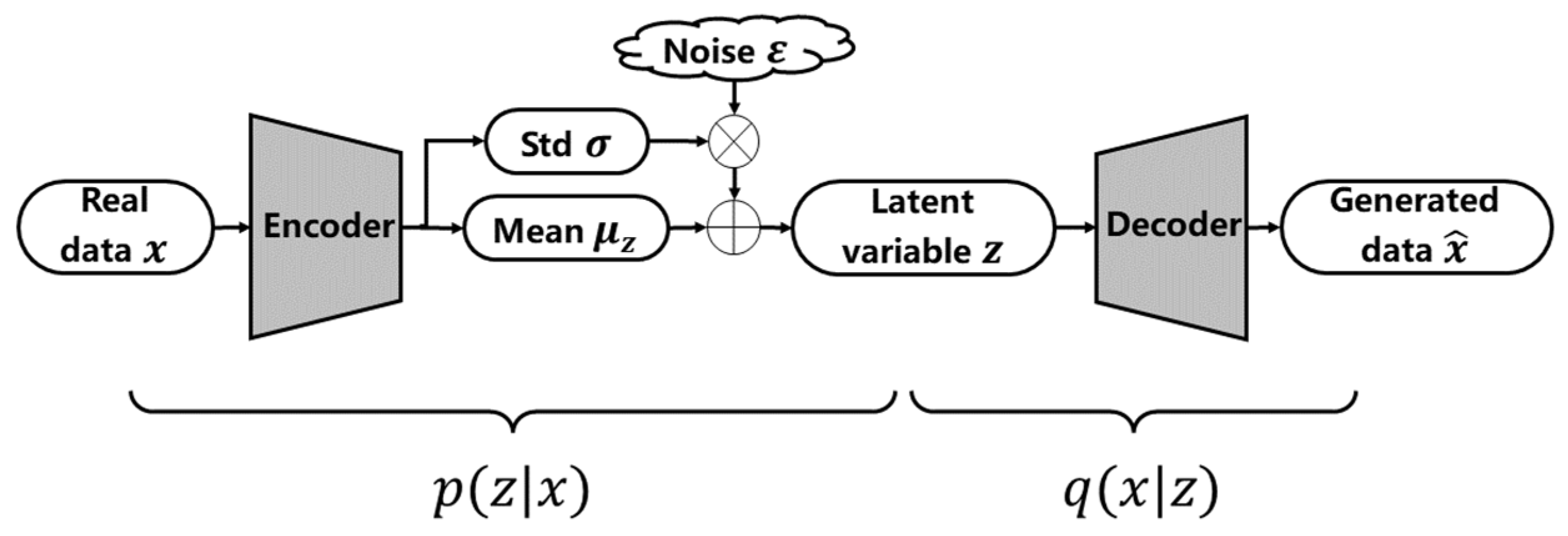
3.2. Bidirectional Autoregressive VAE

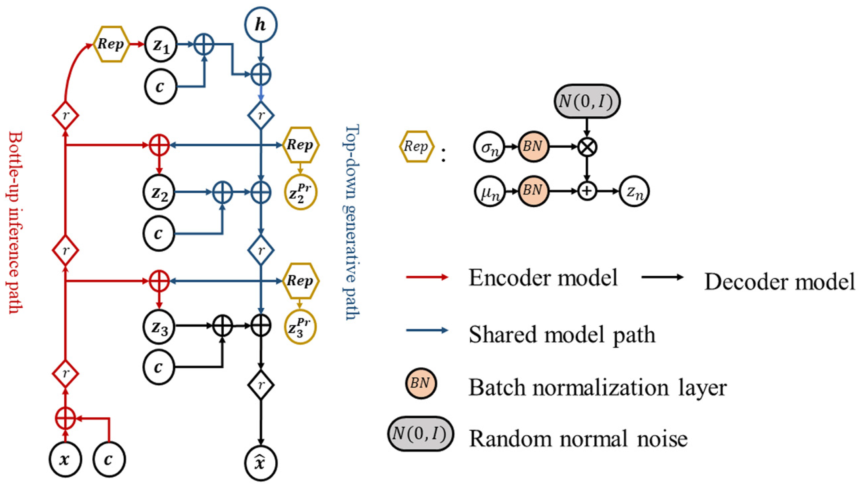
Traditional VAEs apply simple Gaussian priors on latent variables for ease of training. However, these oversimplified distributions limit the ability to generate complex industrial patterns. To address this limitation, we propose a Bidirectional Autoregressive VAE that enhances latent expressiveness through autoregressive modeling. As depicted in Figure 6, BAVAE integrates residual networks into its feature extraction module, structurally improving the decoder’s ability to synthesize high-fidelity industrial signals.

In the Bidirectional Autoregressive VAE, latent variables are partitioned into multiple mutually independent groups:

$$\{z_1,z_2,\dots ,z_L\}$$

(15)

where $L$ denotes the number of groups. The first-layer latent variable $z_1$ is hierarchically conditioned by preceding groups through autoregressive modeling. Higher-layer latent distributions are learned via neural networks. The prior and approximate posterior distributions in BAVAE are formulated as follows:

$$\begin{array}{l}{p}_{\theta }(z)=p_{\theta }(z_1)p_{\theta }(z_2|z_1)\cdots p_{\theta }(z_L|z_{<L})\\ q_{\varphi }(z|x)=p_{\theta }(z_1|x)p_{\theta }(z_2|z_1,x)\cdots p_{\theta }(z_L|z_{<L},x)\end{array}$$

(16)

where the first-layer prior is defined as a standard Gaussian, while subsequent priors follow factorized Gaussian distributions with learnable mean and variance parameters. These parameters are adaptively derived from preceding layers via neural networks, regularized by KL divergence to constrain deviations from the prior. The highest-layer latent distribution is conditioned on all preceding variables and decoded into generated signals, governed by KL divergence and reconstruction loss. The total KL divergence for BAVAE decomposes as follows:

$$D_{\mathrm{KL}}(q_{\varphi }(z|x)\Vert p_{\theta }(z))=D_{\mathrm{KL}}(q_{\varphi }(z_1|x)\Vert p_{\theta }(z_1))+{\displaystyle \sum _{l=2}^L{\mathit{𝔼}}_{q_{\varphi }(z_{<l}|x)}}\left[D_{\mathrm{KL}}(q_{\varphi }(z_l|x,z_{<l})\Vert p_{\theta }(z_l|z_{<l}))\right]$$

(17)

As shown in Figure 6, the architecture of the bidirectional network integrates the encoder and decoder through latent variables. The network on the left, from bottom to top, represents the encoding process. After obtaining the latent variables at each layer, the higher-level latent variables are derived from the encoded information in the preceding layers, moving from top to bottom. Simultaneously, the prior distributions of different latent variables are learned, ultimately decoding into the generated signal.

This autoregressive hierarchy enhances latent expressiveness for complex industrial data generation. The bidirectional design streamlines training by eliminating redundant connections and reducing computational overhead.

Although the proposed BAVAE draws inspiration from hierarchical latent variable models such as Ladder VAE [30] and PixelVAE [31], it differs significantly in both structure and application. In contrast to Ladder VAE’s skip-connections and auxiliary variables, BAVAE adopts autoregressive modeling between latent variable groups in a bidirectional manner. Compared with PixelVAE’s spatial pixel-level dependency for images, BAVAE is tailored to vibration feature sequences and incorporates residual networks for industrial signal generation. Moreover, a feature discrimination loss is introduced to guide the latent representation to be class-sensitive, which is crucial for handling class imbalance in industrial fault diagnosis.

3.3. Enhanced Loss Function

The conventional VAE loss, as shown in Equation (8), jointly optimizes reconstruction fidelity and latent regularization:

$$L_{\mathrm{recon}}={\displaystyle \sum _{n=1}^N\Vert x_n-{\hat{x}}_n{\Vert }^2}$$

(18)

To enhance the discriminability of data generated on imbalanced datasets, this paper introduces a feature discrimination loss function based on the existing two loss functions. Specifically, an additional mapping network is constructed on the basis of the last latent variable layer, comprising global pooling and fully connected layers, with the output being the predicted labels of the latent variables. By widening the gap between samples of different classes during the training process of the Variational Autoencoder, the loss function can be formulated as follows:

$$L_{\mathrm{dis}}={\displaystyle \sum _{n=1}^N{\displaystyle \sum _{k=1}^K\left[-y_{nk}\log ({[f(z_i)]}_k)-(1-y_{nk})\log ({[f(z_i)]}_k)\right]}}$$

(19)

where $f(·)$ denotes the latent mapping function. The composite loss is calculated as follows:

$$L(\theta ,\varphi ;x)=L_{\mathrm{recon}}-\beta L_{\mathrm{DK}}+\alpha L_{\mathrm{dis}}$$

(20)

Here, $\alpha$ and $\beta$ are tunable weights, and $L_{\mathrm{DK}}$ represents the KL divergence in Equation (17). By incorporating $L_{\mathrm{dis}}$, latent representations become class-sensitive during training, enlarging inter-class margins. This facilitates fault classification by generating label-aware synthetic samples, ultimately boosting diagnostic accuracy.

During training, the reconstruction loss ensures the generated samples closely resemble the real samples in the feature space, promoting fidelity. Meanwhile, the feature discrimination loss introduces an additional constraint on the latent space to make the representations more class-discriminative. These two loss components are complementary: while the reconstruction loss focuses on input–output consistency, the discrimination loss pulls latent features apart across classes. The joint optimization drives the BAVAE to generate not only realistic but also class-aware samples, which is crucial for learning under data imbalance.

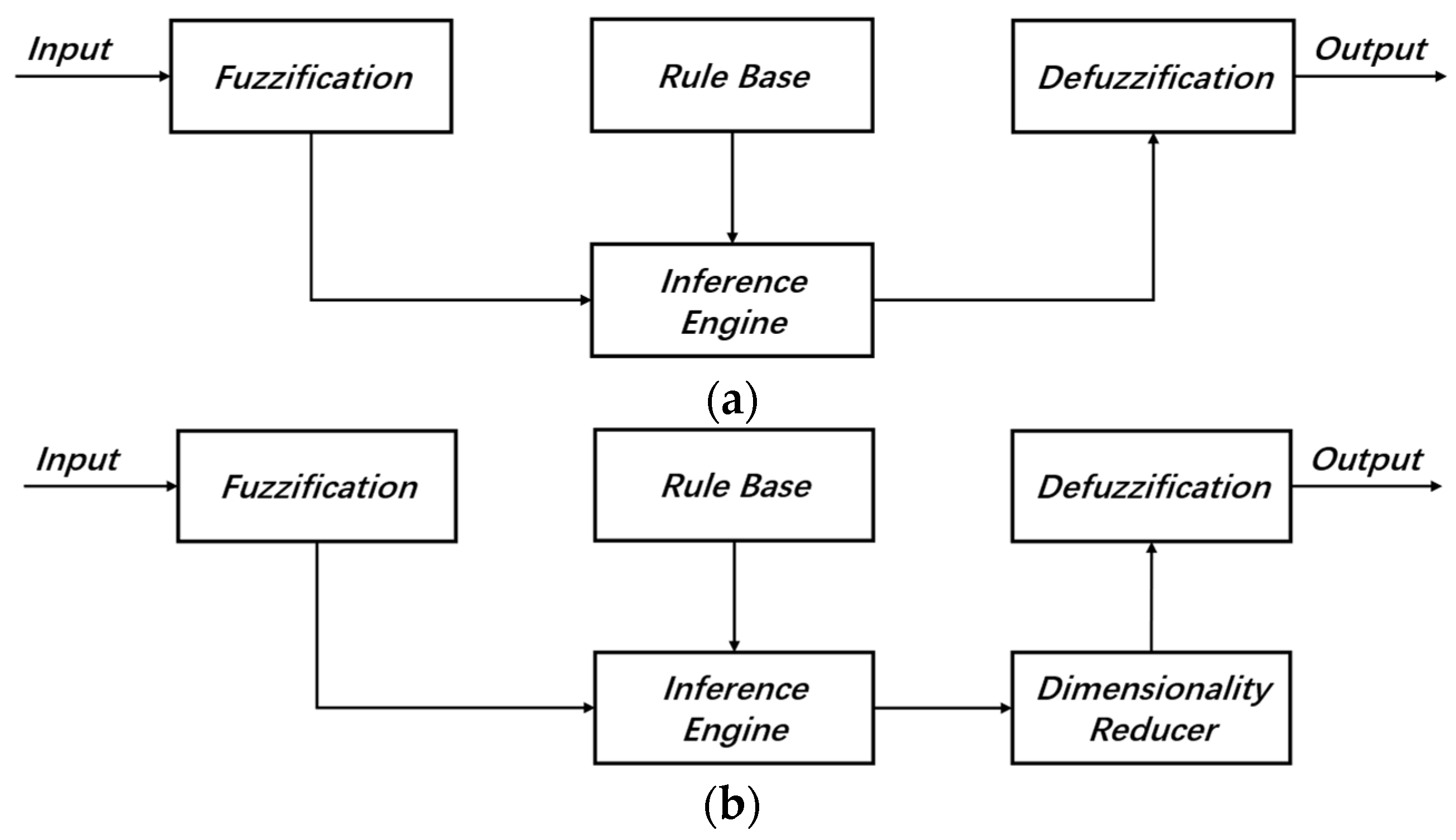
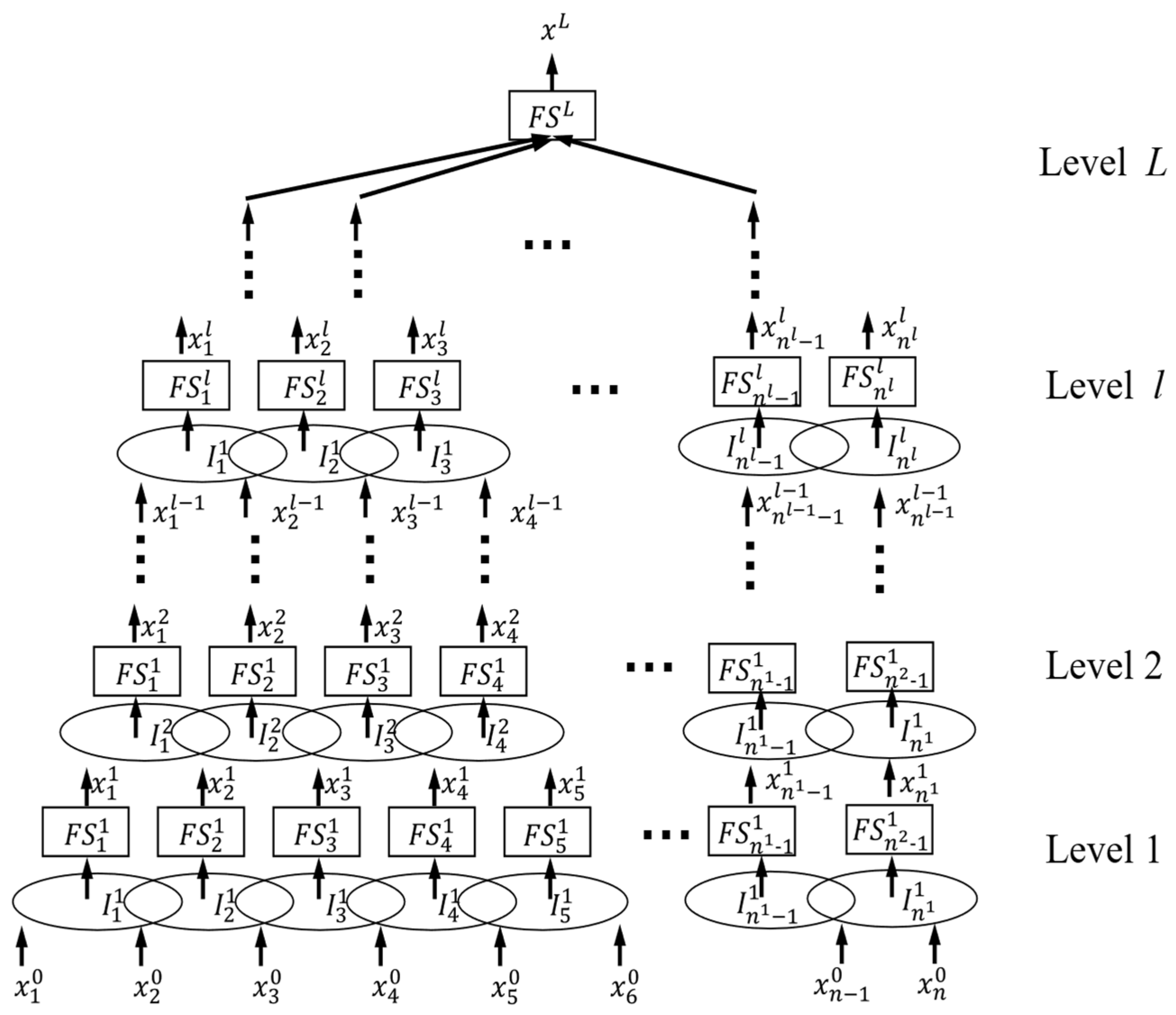
3.4. Deep Convolutional Interval Type-2 Fuzzy System

While data augmentation increases sample quantity, it may fail to address inherent class imbalance in original datasets. Augmented samples often deviate from the true feature distribution of real-world data, leading to biased learning of class distributions. To establish a robust bearing fault diagnosis model, we integrate Interval Type-2 fuzzy systems with deep convolutional networks via a bottom-up hierarchical architecture, as illustrated in Figure 7.

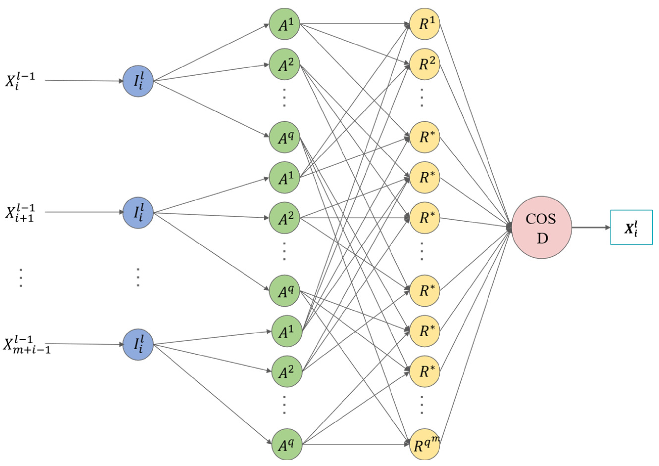
The internal structure of the l-th layer $(l=1,\dots ,L)$ fuzzy subsystem ${\mathrm{FS}}_i^l$$(i=1,\dots ,n^l)$ in the Deep Convolutional Fuzzy System is illustrated in Figure 8. Its input vector is $I_i^l=\left(x_i^{l-1},\dots ,x_{m+i-1}^{l-1}\right)$, where m is a small positive integer. Each input variable is associated with $q(q\ge 2)$ fuzzy sets defined by trapezoidal membership functions:

$$A(x_{*}^{l-1})=\left\{\begin{array}{ll}{\displaystyle \frac{\sigma -|x_{*}^{l-1}-x_{*c}^{l-1}|}{\sigma }},\hfill & x_{*}^{l-1}\in [x_{*c}^{l-1}-\sigma ,x_{*c}^{l-1}+\sigma ]\hfill \\ 0,\hfill & x_{*}^{l-1}\in [\min x_{*}^{l-1},x_{*c}^{l-1}-\sigma ]\cup [x_{*c}^{l-1}+\sigma ,\max x_{*}^{l-1}]\hfill \end{array}\right.$$

(21)

where $x_{*}^{l-1}$ ($*$ denoting any input variable) is the center of the membership function, and $\sigma$ represents the distance from the center to its endpoints. The global minima $\min x_{*}^{l-1}$ and maxima $\max x_{*}^{l-1}$ are determined from training data. The ${\mathrm{FS}}_i^l$ subsystem is governed by $q^m$ fuzzy rules:

$$\begin{array}{ll}{R}^{*}:& \mathrm{IF} x_i^{l-1} \mathrm{is} A^{j_1} \mathrm{and} \cdots \mathrm{and} x_{m+i-1}^{l-1} \mathrm{is} A^{j_m}, \\ & \mathrm{THEN} x_i^l \mathrm{is} B^{j_1,\dots ,j_m}.\end{array}$$

(22)

where $R^{*}$ denotes a rule index, $j_1,\dots ,j_m$ are fuzzy set indices for each of the m input variables, ranging from 1 to q, and $B^{j_1,\dots ,j_m}$ is the output fuzzy set. Defuzzification follows the center-of-sets (COSD) method. The input–output mapping of ${\mathrm{FS}}_i^l$ is as follows:

$$x_i^l=F{S}_i^l\left(x_i^{l-1},\dots ,x_{m+i-1}^{l-1}\right)={\displaystyle \sum _{j_1=1}^q\cdots }{\displaystyle \sum _{j_m=1}^q{c}^{j_1,\dots ,j_m}}{A}^{j_1}\left(x_i^{l-1}\right)\cdots A^{j_m}\left(x_{m+i-1}^{l-1}\right)$$

(23)

Here, $c^{j_1,\dots ,j_m}$ represents the center value of the corresponding fuzzy set $B^{(j_1,\cdots ,j_m)}$, which is also the trainable parameter of ${\mathrm{FS}}_i^l$. $A^{(j_1)}(x_i^{(l-1)})\cdots A^{(j_m)}(x_{m+i-1}^{(l-1)})$ denotes the firing strength of the fuzzy rule shown in Equation (22), denoted as $w^{(j_1,\cdots ,j_m)}=A^{(j_1)}(x_i^{(l-1)})\cdots A^{(j_m)}(x_{m+i-1}^{(l-1)})$.

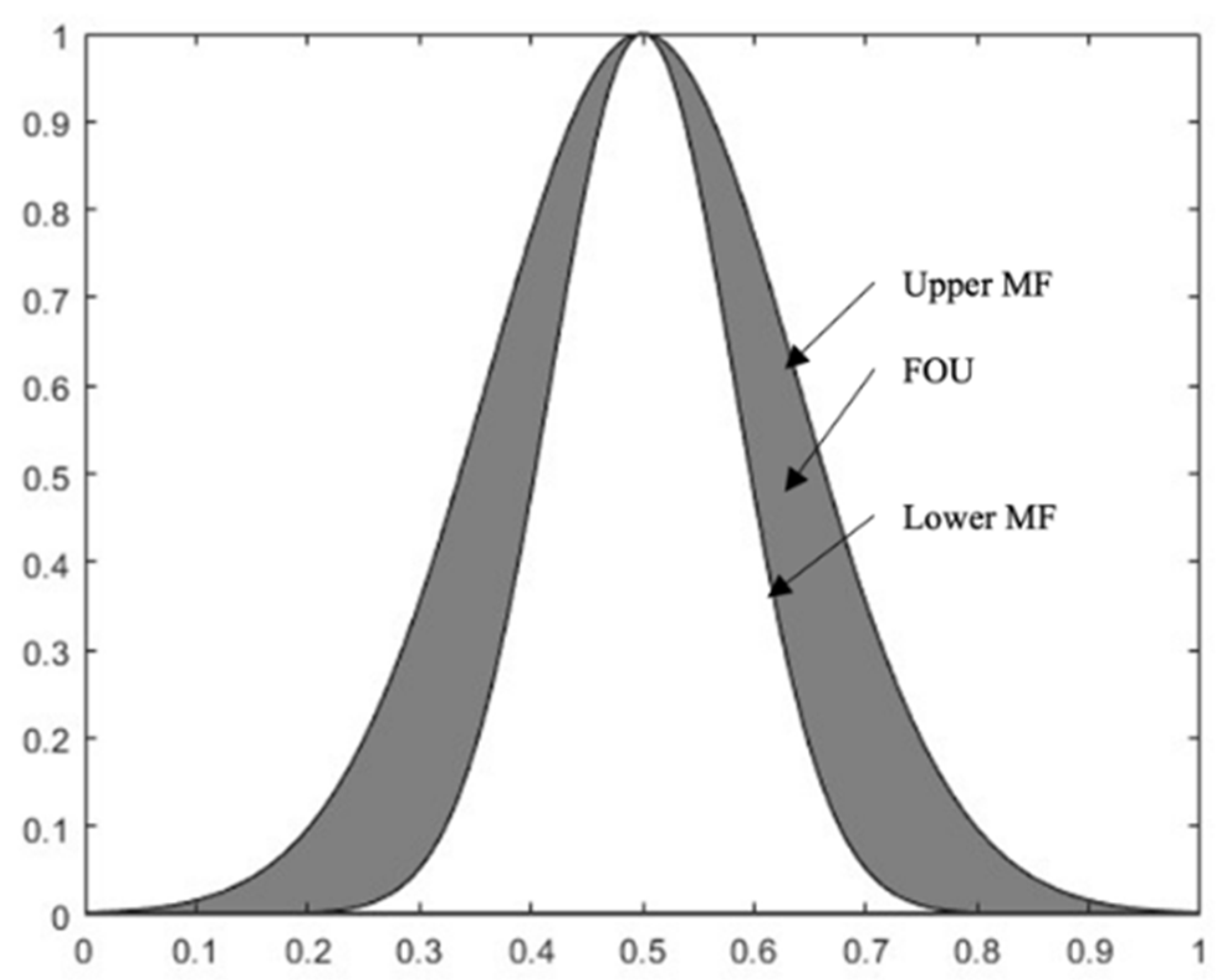
In the formula, the DCIT2FS model for $i=1,2,\dots ,L$ and $s=1,2,\dots ,n$ is a fuzzy system in the Interval Type-2 fuzzy system, where the fuzzy membership function is represented as follows:

$$\begin{array}{l}{A}_1(x(k))=1-{\displaystyle \frac{1}{1+e^{\frac{-(x(k)-{\alpha }_{1^{\prime }})}{{\beta }_1}}}}\\ A_3(x(k))={\displaystyle \frac{1}{1+e^{\frac{-(x(k)-{\alpha }_{3^{\prime }})}{{\beta }_3}}}}\\ A_2(x(k))=1-A_1(x(k))-A_3(x(k))\end{array}$$

(24)

In the equation, $\alpha$ and $\beta$ are two variables of the asymmetric sigmoid function, and ${\alpha }^{\prime }\in [\alpha -\delta ,\alpha +\delta ]$ ($\delta$ is a user-defined constant). Equation (1) illustrates the Interval Type-2 fuzzy rule. This structure forms the foundation for constructing the predictive model DCIT2FS.

$$\begin{array}{ll}{R}^{*}:& \mathrm{if} x_s^{l-1} \mathrm{is} A_1^{*} \mathrm{and} x_{s+1}^{l-1} \mathrm{is} A_2^{*} \mathrm{and} \dots \mathrm{and} x_{s+m-1}^{l-1} \mathrm{is} A_m^{*}\\ & \mathrm{then} {\tilde{y}}^{*}=p_0^{*}+p_1^{*}{x}_1+\dots +p_m^{*}{x}_m\end{array}$$

(25)

In the equation, the variable $A$ is a type-2 fuzzy set. The type-1 fuzzy set describes the polynomial coefficients that follow, denoted as $p$. The conclusion parameter intervals also include predefined upper and lower bounds. The output interval of each rule is calculated as follows ($i=1,2,\dots ,c$):

$${\tilde{y}}^i\in \left[y_i^l,y_i^h\right]=\left[p_{i0}^l,p_{i0}^h\right]+\left[p_{i1}^l,p_{i1}^h\right]x_1+\dots +\left[p_{im}^l,p_{im}^h\right]x_m$$

(26)

The reduction set of the model is an Interval Type-1 fuzzy model,

$$\tilde{y}\in \left[y_i^l,y_i^h\right]=\left[{\displaystyle \frac{{\displaystyle \sum _{i=1}^c{\mu }_i^l}{y}_i^l}{{\displaystyle \sum _{i=1}^c{\mu }_i^l}}}, {\displaystyle \frac{{\displaystyle \sum _{i=1}^c{\mu }_i^h}{y}_i^h}{{\displaystyle \sum _{i=1}^c{\mu }_i^h}}}\right]$$

(27)

The precise output of the model is obtained using the centroid method:

$$\hat{y}={\displaystyle \frac{y^l+y^h}{2}}$$

(28)

Each first-layer fuzzy system is regarded as a weak evaluator that outputs based on only a small subset of input variables. The fuzzy system adopts an IT2 fuzzy model based on an uncertain Gaussian function. The antecedent parameters of this model are optimized using the PSO algorithm.

As the number of features or fuzzy rules increases, scalability becomes an important consideration. To address this issue and maintain computational efficiency, we have implemented several techniques in the proposed DCIT2FS model. When the number of fuzzy rules increases, rule reduction methods, such as K-means or fuzzy C-means clustering, can be used to reduce the number of rules, thus decreasing the computational cost. Additionally, to handle the increase in feature dimensions, we employ feature selection techniques like Principal Component Analysis (PCA) and Mutual Information (MI), which help identify the most relevant features and reduce the dimensionality, thereby alleviating the computational burden. Furthermore, we leverage GPU acceleration during the fuzzy inference process to significantly enhance processing speed, making the model feasible for real-time applications. These strategies ensure that the DCIT2FS model remains scalable and efficient, even as the number of features or fuzzy rules increases, and maintain its applicability in real-time scenarios.

3.5. Proposed Fault Diagnosis Framework

The proposed bearing fault diagnosis framework for imbalanced datasets integrates Deep Convolutional fuzzy systems with Bidirectional Autoregressive VAEs, as illustrated in Figure 9. The key steps are as follows:

(1)

Data preprocessing: The raw data were subjected to outlier detection and denoising. For imbalanced datasets, DTWCT was employed to extract feature values. The extracted features were then concatenated to construct a multi-scale feature training dataset.

(2)

Data augmentation: A BAVAE network model was developed, and hyperparameters were selected accordingly. The network was trained using the multi-scale feature dataset. Noise was sampled from a standard Gaussian distribution to generate synthetic data, which was then combined with real data to train a classification model.

(3)

Model training and fault diagnosis: The augmented dataset was used to train a DCIT2FS. After training, the test dataset was preprocessed and fed into the diagnostic model to complete the fault diagnosis algorithm.

4. Experimental Validation

4.1. Experimental Setup

Experiments were performed using the CWRU bearing dataset to validate the proposed fault diagnosis method. To simulate imbalanced data scenarios, 30% and 50% of samples from each fault class were randomly selected for training, while all normal-condition samples were retained. And wavelet transform was applied to the imbalanced dataset for multi-scale feature extraction, generating an imbalanced feature set.

To better quantify the performance of the proposed algorithm, this paper employs the accuracy metric to provide a comprehensive assessment of its effectiveness. This evaluation metric can be calculated using Equation (29) based on the confusion matrix in

Table 2. Confusion matrix.

True Tag	Prediction Tag
	Positive Example	Negative Example
Positive example	TP (true positive example)	FN (false negative example)
Negative example	FP (false positive example)	TN (true negative example)

.

The accuracy index is calculated as follows:

$$\mathrm{Accuracy}={\displaystyle \frac{TP+TN}{TP+TN+FP+FN}}$$

(29)

4.2. Synthetic Data Quality Assessment

This section demonstrates the generative capability of the Autoregressive Variational Autoencoder (AR-VAE) by comparing the generated features with the true data features. When the data imbalance ratio is 50%, without loss of generality, the data samples of state 8 (fault in rolling element with damage diameters of 0.5334 mm) are selected for analysis. Figure 10a,b show the multi-scale features of the true samples and those generated by the proposed method, respectively. Although there are some differences in detail between the generated multi-scale features and the true sample features, the overall generation effect is satisfactory, which demonstrates that the proposed BAVAE can effectively generate true feature samples. The generated multi-scale features are summed to obtain the original vibration signals.

To more accurately quantify the authenticity of the generated data, this paper employs the inverse of the Fréchet distance as a similarity metric, in combination with CNN as the classifier. Several widely used methods were employed for comparison, including the resampling-based SMOTE [3] and ADASYN [4] algorithms, the Conditional Variational Autoencoder (CVAE), and GAN, as well as BAVAE without the enhanced loss function $L_{dis}$ and BAVAE with the enhanced loss function $L_{dis}$. Both CVAE and GAN were constructed using fully connected layers. And states 1, 2, 3 and 4 were selected for the comparative experiments. The similarity between the data generated by different methods and the true data is compared, as shown in

Table 3. Comparison of similarities between real and generated data.

Method	Similarity
	State 1	State 2	State 3	State 4
SMOTE	0.72	0.79	0.77	0.85
ADASYN	0.75	0.70	0.71	0.88
CVAE	0.88	0.85	0.89	0.92
GAN	0.78	0.82	0.65	0.87
$\mathrm{BAVAE} \mathrm{without} \mathrm{enhanced} L_{dis}$	0.91	0.99	0.93	1.12
$\mathrm{BAVAE} \mathrm{with} \mathrm{enhanced} L_{dis}$	0.94	1.10	0.99	1.19

. The results indicate that the proposed method achieves the highest similarity in generating data across various categories, further validating the effectiveness of the proposed approach in data generation.

The results indicate that the proposed algorithm achieved the best fault diagnosis performance across different imbalance ratios and classifiers, demonstrating its effectiveness. The SMOTE and ADASYN algorithms, based on resampling, can expand the dataset through direct sampling. However, these methods struggle to generate diverse samples within the original data distribution and are highly susceptible to noise interference, resulting in suboptimal data augmentation performance. The CVAE and GAN, built using fully connected layers, have a large number of parameters and overly simplistic structures, making it difficult to generate data that closely resemble real samples. Consequently, their data augmentation effects are limited. The comparative experiments between BAVAE without $L_{dis}$ and BAVAE with $L_{dis}$ further validate the effectiveness of the enhanced loss function $L_{dis}$.

4.3. Case 1: CWRU Dataset

To validate the superiority of the proposed algorithm in fault diagnosis for imbalanced datasets, five diagnostic models were selected to perform fault diagnosis on the augmented dataset. These models include SVM, RF, Convolutional Neural Network (CNN), Deep Convolutional Interval Type-1 Fuzzy System, and the proposed DCIT2FS. The fault diagnosis results for datasets with imbalance ratios of 30% and 50% are shown in

Table 4. Classification accuracy using a 30% imbalance ratio with the CWRU dataset.

Method	Classification Accuracy (%)
	SVM	RF	CNN	DCFS	DCIT2FS
SMOTE	52.34	45.79	91.05	92.10	93.20
ADASYN	54.12	46.52	92.15	93.25	94.50
CVAE	58.76	75.34	90.10	94.50	95.30
GAN	63.21	73.62	88.89	95.60	96.05
BAVAE	79.50	72.10	89.80	96.80	97.00

and

Table 5. Classification accuracy using a 50% imbalance ratio with the CWRU dataset.

Method	Classification Accuracy (%)
	SVM	RF	CNN	DCFS	DCIT2FS
SMOTE	72.13	75.28	92.17	93.52	95.08
ADASYN	72.85	74.14	92.39	93.79	95.37
CVAE	80.96	76.18	93.07	96.02	97.03
GAN	80.99	81.03	93.51	96.38	97.46
BAVAE	83.57	84.00	94.67	97.33	98.67

. For the SVM and RF models, default parameter settings were used. The CNN model was constructed using only conventional convolutional and pooling layers.

From the data in Table 4 and Table 5, it is evident that the BAVAE method outperforms other methods in classification accuracy under different imbalance ratios (30% and 50%), especially with the DCIT2FS and DCFS classifiers, where it shows particularly outstanding performance. At a 30% imbalance ratio, BAVAE achieves higher accuracy across all classifiers compared to other methods, with DCIT2FS reaching an accuracy of 97.00% and DCFS reaching 96.80%. When the imbalance ratio increases to 50%, BAVAE’s overall accuracy improves further, especially with DCIT2FS, which achieves 98.67%, demonstrating stronger generalization ability and stability compared to other methods. In contrast, GAN and CVAE perform well with certain classifiers, particularly GAN in RF and CNN, but still fall short of BAVAE. Traditional oversampling methods like SMOTE and ADASYN have lower overall accuracy; although there is some improvement in the CNN classifier, their performance in other classifiers remains significantly behind. Overall, the proposed BAVAE-DCIT2FS method achieves the best classification results in all experimental settings, proving its superiority in handling imbalanced datasets, especially when combined with the DCIT2FS classifier, which leads to the highest classification accuracy, showcasing strong data generation and adaptation capabilities. Figure 10 and Figure 11 present the confusion matrices for five algorithms combined with BAVAE on a 50% imbalanced dataset. The results indicate that SVM and RF perform relatively poorly, while DCFS and DCIT2FS show better performance. Notably, the introduction of the Interval Type-2 fuzzy system into DCFS, resulting in DCIT2FS, leads to superior diagnostic performance, further validating the effectiveness of the proposed DCIT2FS diagnostic model.

Figure 12 indicates that the proposed method provides accurate diagnostic results for most categories, with only a small number of diagnostic errors in a few categories. The above experiments validate the data generation capability of the proposed BAVAE, as well as the fault diagnosis capability of the proposed BAVAE-DCIT2FS method on imbalanced datasets.

4.4. Case 2: Wind Farm Dataset

Although testing with the CWRU dataset has already demonstrated the superiority of our proposed method, the dataset is quite simple and not affected by substantial noise. In this section, the vibration data from a real wind farm are collected to evaluate our proposed method. The data were provided by a company for us to study and design a customized wind turbine prognosis and health management system with the aim of lowering maintenance costs. The data were acquired from wind turbine (WT) gearboxes using a special CMS and data acquisition station, as shown in Figure 13. Based on long-term recordings of the company, there are three parts of the gearbox that are more vulnerable than other components: high-speed shaft bearings, middle-speed shaft bearings, and planetary gears. Since wind power generators are often built in remote districts and far from each other, inspections by personnel involve high financial and labor costs. Thus, an intelligence-based system is quite urgent to monitor health conditions and predict impending failures of gearboxes.

The data were collected from different WT gearboxes and then segmented and labeled by expert inspection workers with the following classes: Normal Condition (NC), High-speed Shaft Bearing Damage (HSBD), Middle-speed Shaft Bearing Damage (MSBD), and Planetary Gear Damage (PGD). Similarly, 540 samples of each class were selected, each with 1020 data points. Imbalance ratios of 30% and 50% per class were used in the training set. The initialization and parameters of the experiment are the same as Case 1. The experimental results are shown in

Table 6. Classification accuracy using a 30% imbalance ratio with a wind farm dataset.

Method	Classification Accuracy (%)
	SVM	RF	CNN	DCFS	DCIT2FS
SMOTE	50.12	43.85	89.34	90.45	91.80
ADASYN	52.67	45.41	90.12	91.25	92.40
CVAE	56.03	70.11	88.45	92.60	93.15
GAN	60.24	70.25	87.90	93.10	94.05
BAVAE	75.38	68.90	87.65	94.45	95.10

and

Table 7. Classification accuracy using a 50% imbalance ratio with a wind farm dataset.

Method	Classification Accuracy (%)
	SVM	RF	CNN	DCFS	DCIT2FS
SMOTE	70.12	72.45	90.34	91.90	93.60
ADASYN	71.05	71.30	90.85	92.20	94.10
CVAE	78.24	73.02	91.40	94.20	95.50
GAN	78.80	78.25	92.15	95.10	96.80
BAVAE	81.35	80.60	93.02	96.55	97.40

, respectively.

Since the wind is unpredictable, the data collected from gearboxes in wind turbines are highly nonstationary and feature irregular noise. However, compared with other methods, our method still achieves reasonable performance on complex data, which verifies the feasibility of our method in an actual wind farm.

5. Conclusions

This paper proposes a novel fault diagnosis framework based on a BAVAE and a DCIT2FS to address the challenges associated with imbalanced bearing fault datasets. In the first stage, multi-scaled features of each class are extracted and concatenated through DTCWT as input data. The BAVAE improves the diversity and quality of generated samples by iteratively learning complex latent distributions and introducing a feature discrimination loss, which effectively enhances inter-class feature distinctions. When combined with the original dataset, this augmentation strategy significantly boosts the robustness of the diagnostic model. Additionally, the DCIT2FS capitalizes on the powerful approximation capabilities of Interval Type-2 fuzzy systems and the hierarchical feature extraction provided by deep convolutional networks. This combination achieves a favorable trade-off between model complexity and feature representation, thereby improving diagnostic performance under uncertain and imbalanced conditions. Experimental results on the CWRU dataset demonstrate that the proposed framework outperforms several state-of-the-art methods in terms of diagnostic accuracy and stability. The generalization capability of the proposed algorithm was validated using a wind farm dataset.

However, there are still areas that warrant further investigation. Future research will focus on developing more advanced feature fusion mechanisms to fully integrate multi-scale and multi-modal data. Additionally, we aim to enhance the generative capacity of BAVAE in extremely imbalanced and noisy industrial environments. Furthermore, combining advanced deep learning models with traditional signal processing techniques to address the complexities of industrial big data will remain a key direction for both theoretical research and practical applications.