1. Introduction
The contact forces at the wheel–rail interface are the result of the vehicle’s weight, acceleration, braking, and steering forces [
1]. If stresses in the contact areas are greater than the plastic yield limit, the material experiences plastic deformation. Pearlitic steel is the common material used in manufacturing rails and wheels in Europe [
1]. The mechanical characteristics of pearlitic steel are highly dependent on its microstructural features. For pearlitic steel, the interlamellar spacing is a critical microstructural feature. There is a correlation between the interlamellar spacing and the steel’s strength, as demonstrated by Dollar et al. [
2]. Bouaziz et al. [
3] also developed a relationship to predict the effect of the interlamellar spacing on the flow stress. Grain size is one of the parameters that can influence the mechanical properties of pearlitic steel. The Hall–Petch relation is one of the most well-known relationships describing grain size’s effect on yield strength [
4]. Pearlitic steel shows mechanical properties resulting from the mixture of ferrite and cementite, making it strong and resistant to wear without being too brittle; therefore, it can withstand the heavy cyclic loads experienced by railway infrastructure [
1].
The contact zone between train wheels and rails is tiny, resulting in high contact pressures that can cause localized severe plastic deformations (SPDs) near the surface. Cracks originate mainly from the highly deformed regions below the surface [
5]. Improving the crack growth model’s reliability and accuracy in SPD regions can increase maintenance planning reliability and traffic safety [
6]. Scientists have developed techniques to produce severely deformed microstructures, such as high-pressure torsion (HPT) [
7]. The scheme for creating a severely plastically deformed microstructure through the HPT process involves applying substantial torque and hydrostatic pressure to a disk-shaped sample. The usual experimental approach to investigate the effect of severe plastic deformation on the mechanical properties of railway material is to find a relationship between the microstructure, mechanical properties, and the local strain for lab-produced severely deformed microstructure or worn rails [
8,
9,
10,
11,
12]. The effect of SPD microstructure on fatigue behavior has also been widely researched experimentally [
13,
14,
15,
16,
17,
18,
19].
Additionally, the effect of plastic deformation on fatigue life was investigated numerically using a parameter that accounts for microstructural characteristics [
20,
21]. The T-γ model [
22] was developed to predict crack initiation using damage function. The finite element method, FEM, combined with cohesive zone modeling, is often used for modeling fatigue crack growth in the literature [
23]. Vijay et al. [
24] developed a 3D FEM model to analyze the anisotropy in rolling contact fatigue as a result of anisotropic material properties (randomness) in crystals. Integrating cohesive zone modeling and extended finite element methods enabled Dekker et al. to model crack growth in arbitrary paths [
25]. Arata et al. [
26] used the cohesive zone modeling method to investigate the crack path within the lamellar structure of titanium aluminide grains. Another alternative approach to model fatigue crack growth is to use the crack growth resistance function in the domain of interest. With the help of such functions, Larijani et al. [
27] developed a model to calculate the fatigue crack growth rate anisotropy in near-surface layers of deformed wheel materials without explicitly considering microstructural features. Nezhad et al. [
28] developed a 3D finite element model to predict the rolling contact fatigue (RCF) crack growth direction and rate in railheads under combined stress and thermal loading.
Other than FEM, some methods are capable of modeling crack growth, such as the discrete element method (DEM) and Peridynamic model. The DEM is typically used for granular materials. However, it can be employed to model solid-state materials. The discrete element method was first introduced by Cundall and Strack in 1979 to analyze granular material [
29]. The DEM is a strong computational method for discontinuous material [
30,
31,
32,
33,
34]. Raje et al. [
35,
36,
37] used the soft contact discrete element model (which is in the family of the DEM) to investigate RCF in roller bearings. Januschewsky et al. [
38] developed a DEM model capable of predicting the rolling contact model (RCF) with a novel bond law considering crack closure behavior.
This research presents a method to predict the fatigue crack growth (FCG) rate via DEM in deformed and undeformed microstructures of pearlitic steels. The model is designed to account for the impact of plastic deformation during service life on the microstructure and behavior of cracks. The model employs a hierarchical mesh introduced by Davoodi Jooneghani et al. [
39]. In the hierarchical mesh, each layer represents a distinct microstructural feature. The model combines the DEM and damage criteria. This combination allows for the prediction of the crack growth rate. The influence of plastic deformation on the FCG rate is determined to be substantial, and this outcome is further analyzed by comparing it with crack growth rate data for a particular variant of pearlitic steel, identified as R260, as documented in existing research. The developed model can connect microstructural features and plastic deformation with the material’s fatigue behavior during cyclic loading.
4. FCG Modeling Using DEM
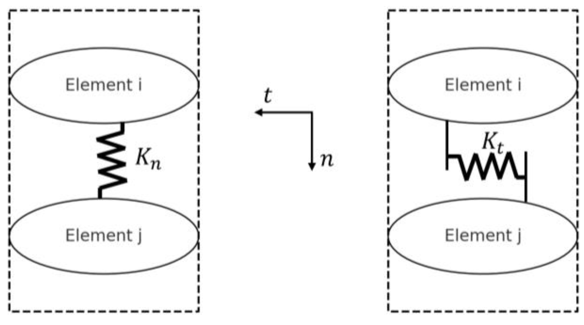
DEM is an appropriate approach to model fatigue crack growth in undeformed and shear-deformed microstructures because the microstructure can be explicitly considered. A DEM simulation is needed to calculate the stress field around the initial crack in the domain, which ultimately results in fatigue crack growth. The material is modeled in DEM as discrete, rigid entities interacting at their interfaces. Such interactions are modeled with springs, which link the elements together. The springs that join the elements are the only parts that deform; the elements do not deform. A two-element DEM setup is shown in
Figure 4. Two discrete elements,
and
, are in contact in this setup. The contact between these elements is modeled using springs in normal and tangential directions. The springs in the normal direction control the compressive and tensile interactions, while the tangential springs are responsible for the shear interactions between the elements. Here,
and
are the stiffness properties in these springs’ normal and tangential directions, respectively. The springs’ stiffnesses will degrade as a response to load cycles, following the applied damage law, and eventually, a crack will form.
The springs in a general DEM model can also exhibit damping properties. This damping usually takes the form of damping coefficients that scale with the springs’ stiffnesses. In the current work, damping is not included in the interface formulation. This simplification was used to isolate the measurement of the material’s static behavior because only the quasi-static results are of interest for the current study.
The stiffness values in the normal (
) and tangential (
) directions in the DEM are derived by integrating the distributed local stiffness along the contact surface length in
and
. By integrating these local stiffness values over the length of contact (
), the global stiffness parameters,
and
, for the interface are obtained. To derive the governing equilibrium equation in the DEM, two contacting elements,
and
, were considered. When an external load is applied, deformation occurs in the contacting springs between these two elements (see
Figure 5). In this figure,
represents the center of the contact interface between elements
and
.
is the point located on element
at the distance of
from
.
is the point located on element
, which was in contact with
prior to any deformation. Other parameters will be clarified in the following paragraphs.
The normal force
and the tangential force
can be described as follows in Equations (1)–(4), based on
Figure 5:
where
represents the distributed stiffness of the spring connecting elements
and
. Furthermore,
is the normal component of
, which describes the fiber stretch connecting two points
and
in
Figure 5. This normal displacement component is used to calculate the normal force generated in the spring, accounting for the stiffness and relative displacement between the elements.
Tangential force resists the sliding motion between the elements like the normal force resists compression or separation. The tangential force can be calculated by Equation (4).
where
and
represent the displacements of the springs at the midpoint of the contact face in the normal and tangential directions for element
, which is in contact with element
.
is the rotational stretch of spring at the distance of
.
and
are the rotational displacement at elements
and
. To proceed, it is necessary to relate
and
to the displacement of the center point of elements. The displacements of the center point of elements
and
are shown in Equation (5).
where
,
, and
are displacements in global coordinates in the
and
directions and rotational displacement of the element.
The displacements of the springs at the midpoint of the contact face are described in Equations (6) and (7).
where
is defined as a unit vector perpendicular to the vector connecting the center point of element
to the midpoint of the contact face between elements
and
(see
Figure 6).
is the component of
in the
direction and
is the component of
in the
direction.
To project the displacement vector
in normal and tangential directions, the step shown in Equation (8) was taken.
where
is the dot product,
is the component of a normal vector (
) in the
direction, and
is the component of a normal vector in the
direction. Similarly, the projection of the displacement vector
in tangential directions is achieved with Equation (9).
Therefore, the following expressions in Equations (10) and (11) for the normal and tangential components of the force were obtained.
Given the displacements of the two contacting elements
and
, the force acting on the surface between these two elements can be calculated. Additionally, momentum (or torque) acting on the surface must be considered. The momentum should be calculated around the center point of the element. The momentum around the element center point is calculated as in Equation (12).
where
in Equation (13) is the momentum resulting from concentrated forces acting on the contacting surface between elements
and
;
is the momentum resulting from distributed forces acting on the contacting surface between elements
and
; and
is the momentum around the center point of the element.
where
is the cross-product and
is the lever vector shown in
Figure 6. This equation translates the local momentum from the contact face to the element’s center by adding the moment caused by the distance between the two points. Therefore,
can be expressed as Equation (14).
In Equation (14),
,
, and
are the stretch of the spring due to displacement in the normal, tangential, and rotational directions. By expanding Equation (14), Equation (15) was obtained.
Until now, the forces and the momentum acting on element
due to contacting element
were calculated. However, in the meshes, element
has contact with several other elements. The other contacting elements are as
,
, ……, and
, assuming that element
has contact with
other elements. To achieve equilibrium for element
, the sum of all forces and moments due to contacts with each neighboring element must be balanced. Therefore, for the equilibrium of the element in the global
,
, and rotational directions, Equations (16)–(18) can be used.
In Equations (16)–(18), the contacting elements (
,
, ……, and
) should be known. To improve efficiency, a faster method [
36] for finding the contacting elements is employed by restricting the search region to the immediate vicinity of the element. The details of this method can be seen in
Figure 7.
To solve Equations (16)–(18) for a mesh containing elements, they can be rewritten in a more generalized matrix form, which will help to facilitate the solution process. As mentioned earlier, it has already been identified that the contacting elements (, , ……, and ) are for element . For a system with elements, Equations (19)–(21) can be expressed.
,
, and
(
) are calculated from the expansion of equations considering all the contacting elements. To solve Equations (19)–(21), they were organized like a stiffness matrix in equilibrium analysis. Just like in a traditional stiffness matrix formulation, where the relationship between forces and displacements is represented through a global matrix equation, it can be described as the equilibrium of forces and moments acting on elements as Equation (22).
where
is the stiffness matrix that incorporates the interaction between all contacting elements. This matrix would include contributions from the neighboring elements (
,
, ……, and
) in contact with element
. Vector
represents the unknown displacements, and
represents the forces acting on the elements due to the forces at the boundaries of the mesh domain. If
matrix is expanded and no boundary forces are assumed, Equation (22) can be expressed in its expanded form as Equation (23).
Normal and tangential stiffness calibration directly impacts stress and strain calculation. As a result, many studies have focused on calibrating these stiffnesses to enhance the prediction of stress and strain for different materials in DEM. Following the findings of Raje et al. [
36], the stiffness values as detailed below in Equations (24) and (25) were selected. In this context,
represents the distance between the centers of elements
i and
j, projected along the normal direction, and
is the thickness of the elements,
is the elastic modulus, and
is the Poisson’s ratio.
The stress near the initial crack is calculated in the model by applying a force to the domain’s boundary. The magnitude of the applied force is determined based on available data from the literature, which are in the form of stress intensity factors. Linear elastic fracture mechanics principles convert stress intensity factors into boundary forces. The corresponding boundary forces were calculated to match the stress intensity factor values reported in the literature. Then, based on the damage law proposed by Raje et al. [
36], the springs’ stiffnesses will degrade as a response to load cycles, leading to crack propagation from the initial crack (see Equations (26) and (27)). A damage parameter D is defined and assigned to each interface. Initially, D is set to zero, and it gradually increases to a maximum value of 1 as load cycles progress.
where
and
are the initial stiffnesses in the normal and tangential directions.
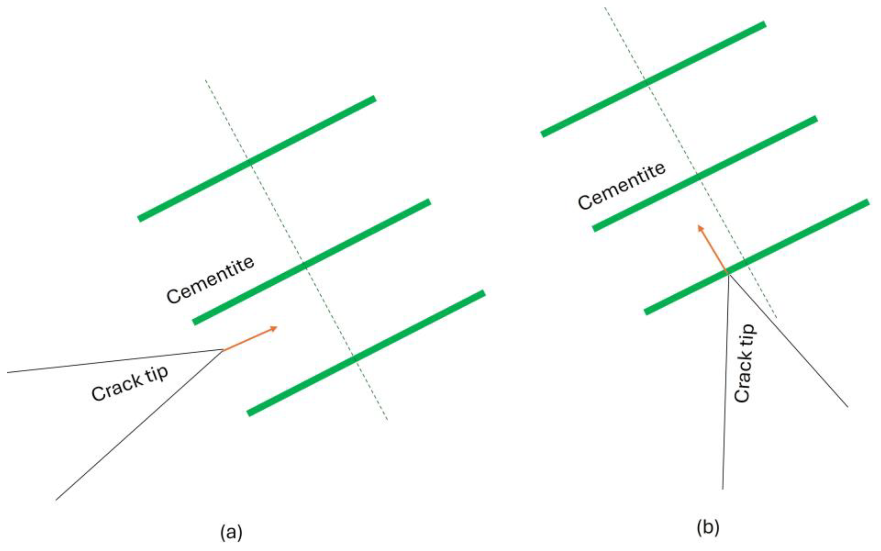
The damage parameter must increase with load cycles and the amplitude of applied stresses at the interface. For a damage law suitable for the proposed meshing methodology, it is essential to account for the multi-layered mesh structure. Since crack growth behavior differs based on whether it grows along or breaks through cementite lamellae, two distinct conditions are proposed: one for when the crack propagates along the cementite layers and another for when it penetrates through them (see
Figure 8).
When a crack grows alongside the cementite and ferrite interface, as shown in
Figure 8a, the following power–law relation is proposed for the rate of damage evolution in an interface. This relation combines the ideas and approaches of the Peridynamic fatigue cracking model of Silling and Askari [
43] and the fatigue threshold model of Lucas and Gerberich [
44].
In this context,
represents the damage evolution at the interface due to the normal stress
acting on it. Here,
is the material’s yield stress,
is a constant,
is the length of the contacting interface, while
is the threshold stress below which the crack does not propagate. The stress of the threshold may also depend on other material properties. Similarly, the damage evolution when the stress is tangential to the interface of ferrite and cementite (damage because of tangential stress (
)) can be defined.
Equations (28) and (29) apply when the crack propagates along the interface between cementite and ferrite. However, when the crack breaks through the cementite lamellae, it must overcome stress greater than
due to the higher strength of the cementite. In this scenario, the crack must surpass critical stress (characteristic strength of cementite (
)), representing the strength required to fracture the cementite, typically exceeding the yield stress. For this case, Equations (30) and (31) govern the damage evolution under normal and tangential loading conditions.
Thus, after calculating the separate damage evolutions for normal and tangential loads, the overall damage evolution can be determined as in Equation (32).
It is worth noting that, for other interfaces within the mesh, such as block, colony, and PAG boundaries, Equations (28) and (29) are used because a crack propagating through these interfaces does not require cementite breakage.
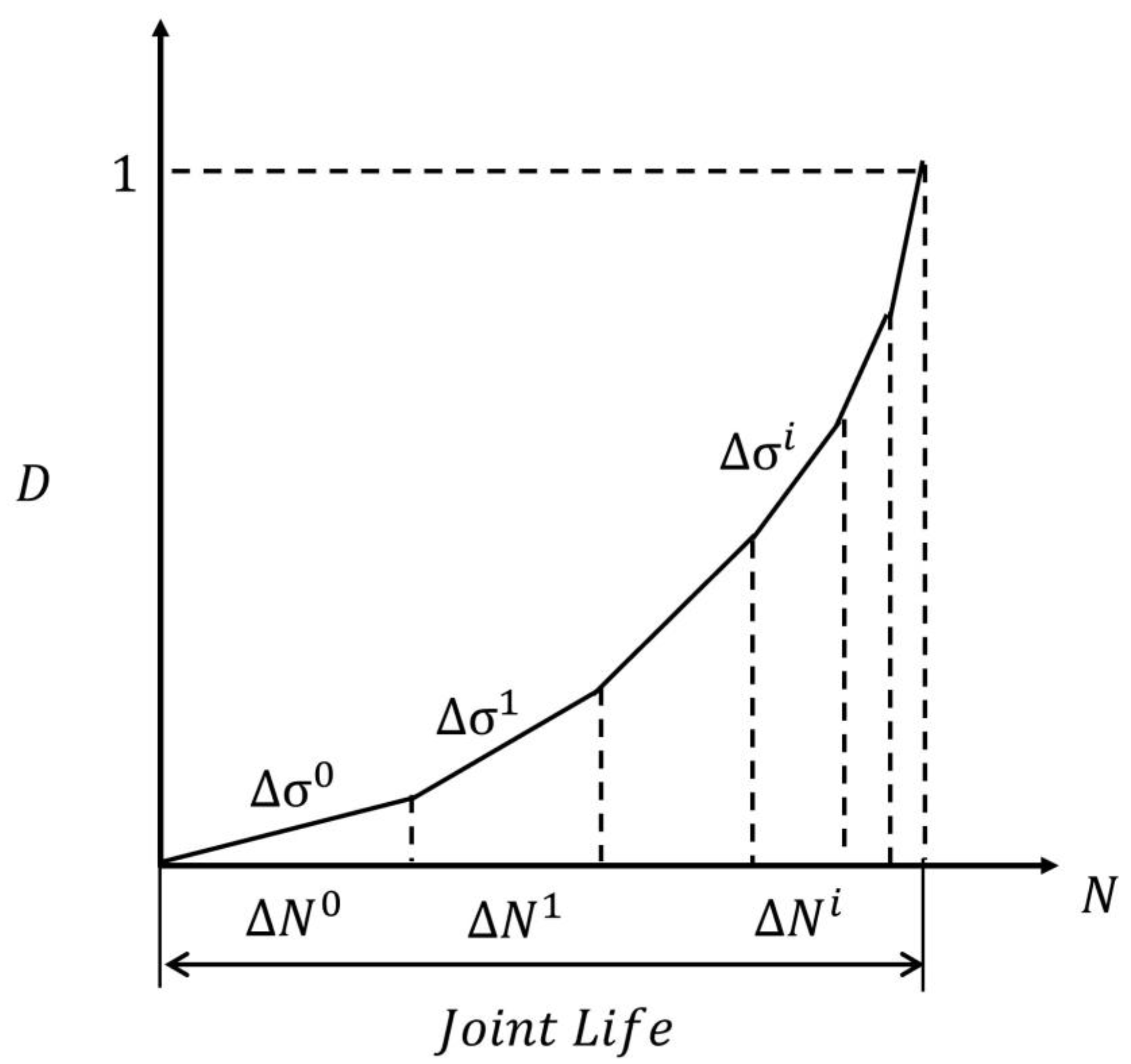
Once damage parameter
reaches a value of 1, a crack propagates along the interface, requiring multiple load cycles. Simulating each load cycle, however, is computationally time-consuming. Therefore, the jump-in-cycles method, described by [
36], is used to model fatigue damage. This method applies a small increment,
, to the damage variable for each cycle block,
, while keeping the stress level constant (
Figure 9).
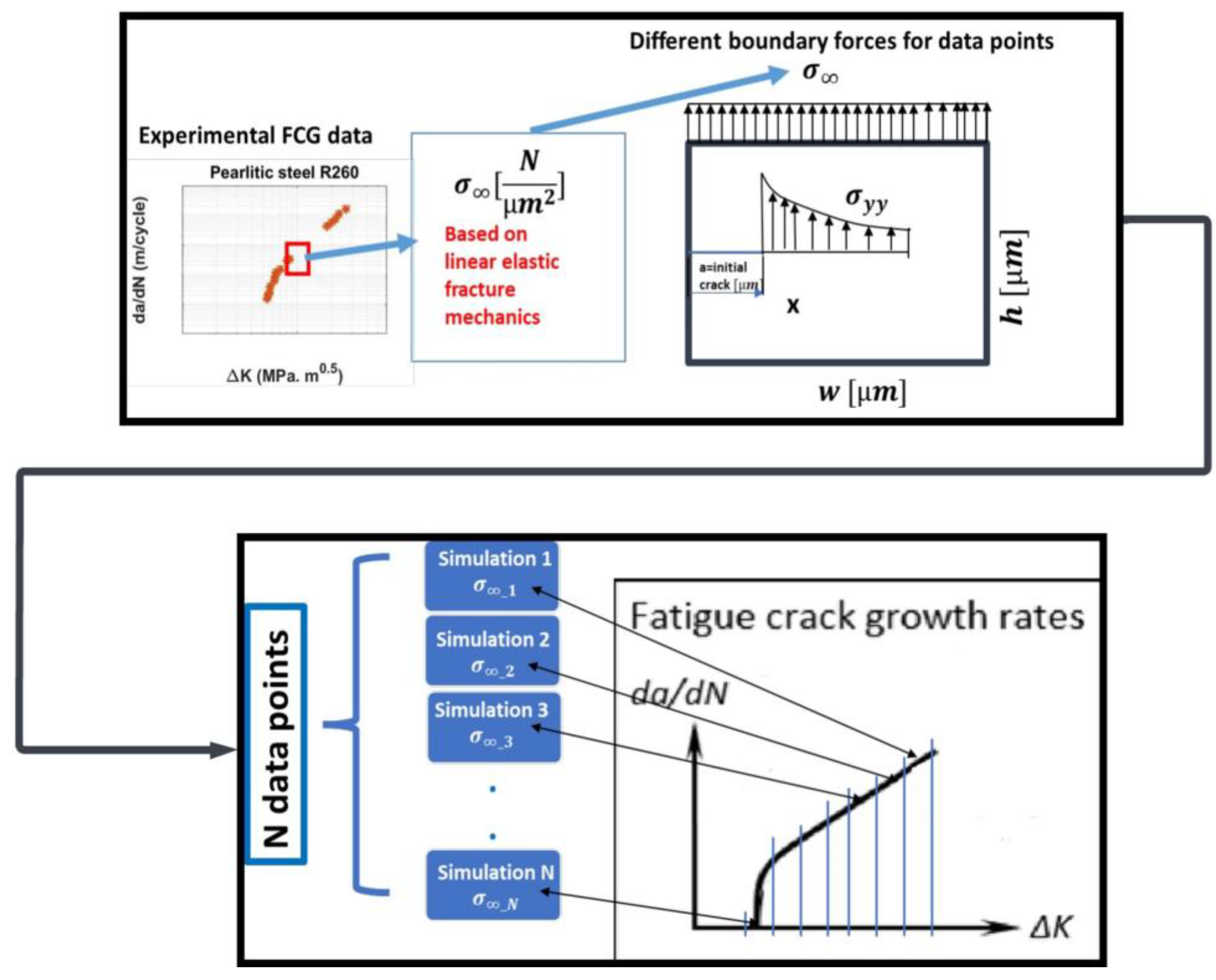
When the desired crack length is reached by degrading several interfaces, the average slope of crack length versus the load cycles graph is calculated. This slope represents the crack growth rate under the specific load value related to the applied stress or stress intensity factor. This procedure is repeated for multiple data points (different load values), and each crack growth rate is used in the fatigue crack growth (FCG) graph. The structure of the calculation is shown in detail in
Figure 10. As previously described and shown in this figure, the boundary stresses in the simulation (
) are chosen based on the target stress intensity factors using linear elastic fracture mechanics (LEFMs). A crack growth simulation is performed for each selected boundary stress (data point) until the desired crack length is reached. The crack growth rate for each data point is then recorded. By repeating the procedure for
data points, the final fatigue crack growth rate diagram can be plotted.
5. Results and Discussion
The meshes described in
Figure 2 and their repetitions were used in the DEM model. For the simulation process, damage model parameters must be chosen for each level of deformation. The damage model explained in Equations (28)–(32) was calibrated to match the undeformed state and tested and validated for both moderately deformed and severely deformed states. For determining the yield stress,
, in the damage model, the research by Tomlison et al. [
45] was used. In their study, they modeled the yield stress as a function of the shear strain (
) using Equation (33) for R260.
By using Equation (33), the yield stress for the undeformed state was calculated to be
, for moderately deformed (
),
, and for severely deformed (
),
. The threshold stress (
) can be derived proportional to the stress intensity factor threshold (
) with the help of previously mentioned linear elastic fracture mechanics (LEFMs). The values for
for different deformation states are
for undeformed,
for moderately deformed (
), and
for severely deformed (
) based on the experiments conducted by Leitner et al. [
18,
19,
40]. The characteristic strength of cementite (
) is approximately
based on the research conducted by Garvik et al. [
46].
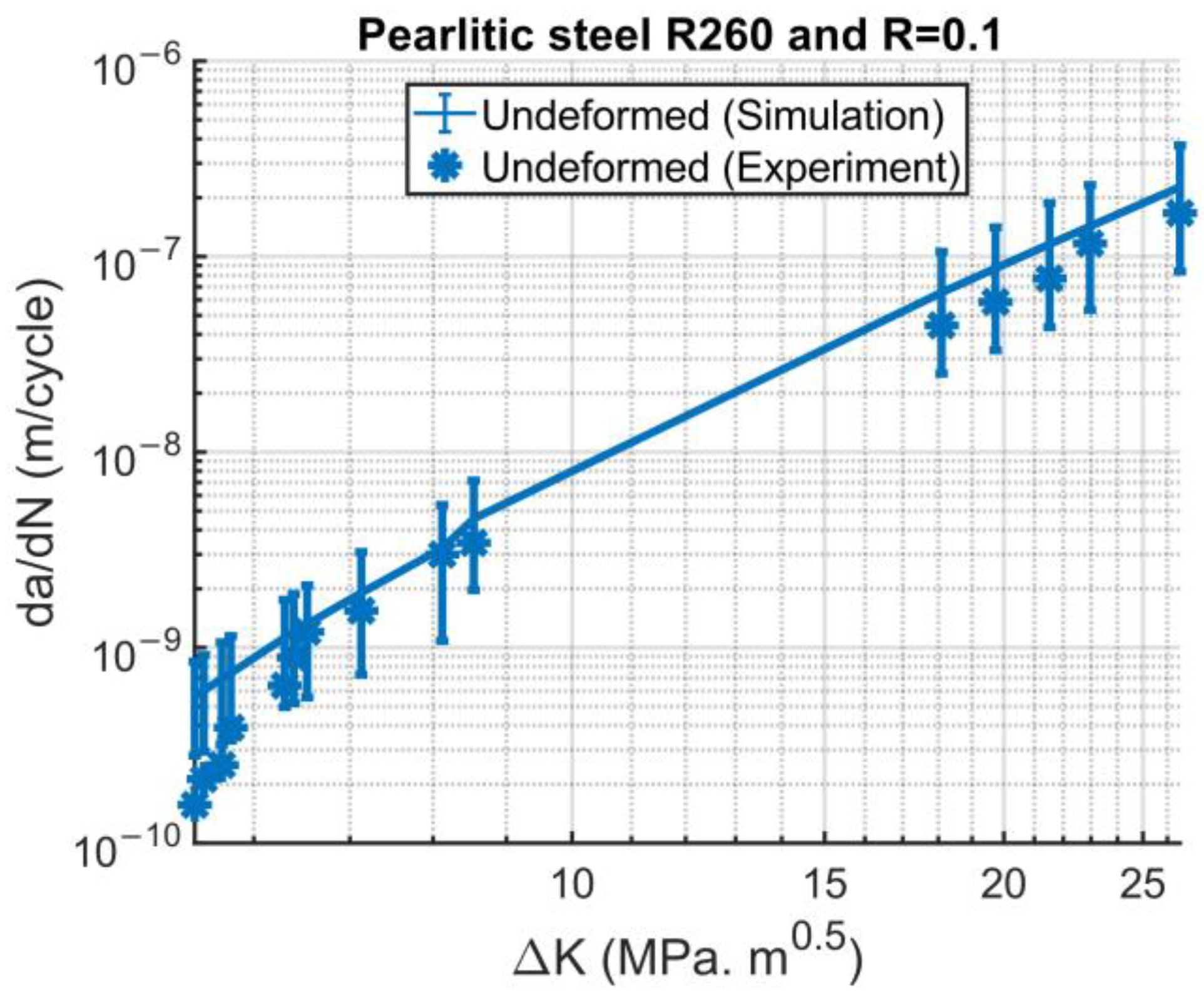
and
in Equations (28)–(32) were fitted for the undeformed state (see
Figure 11) to be
and
, and were used to validate other deformation degrees. The results exhibit scattering, according to the range shown by the error bars in
Figure 11. This scattering is likely due to inherent randomness in the model.
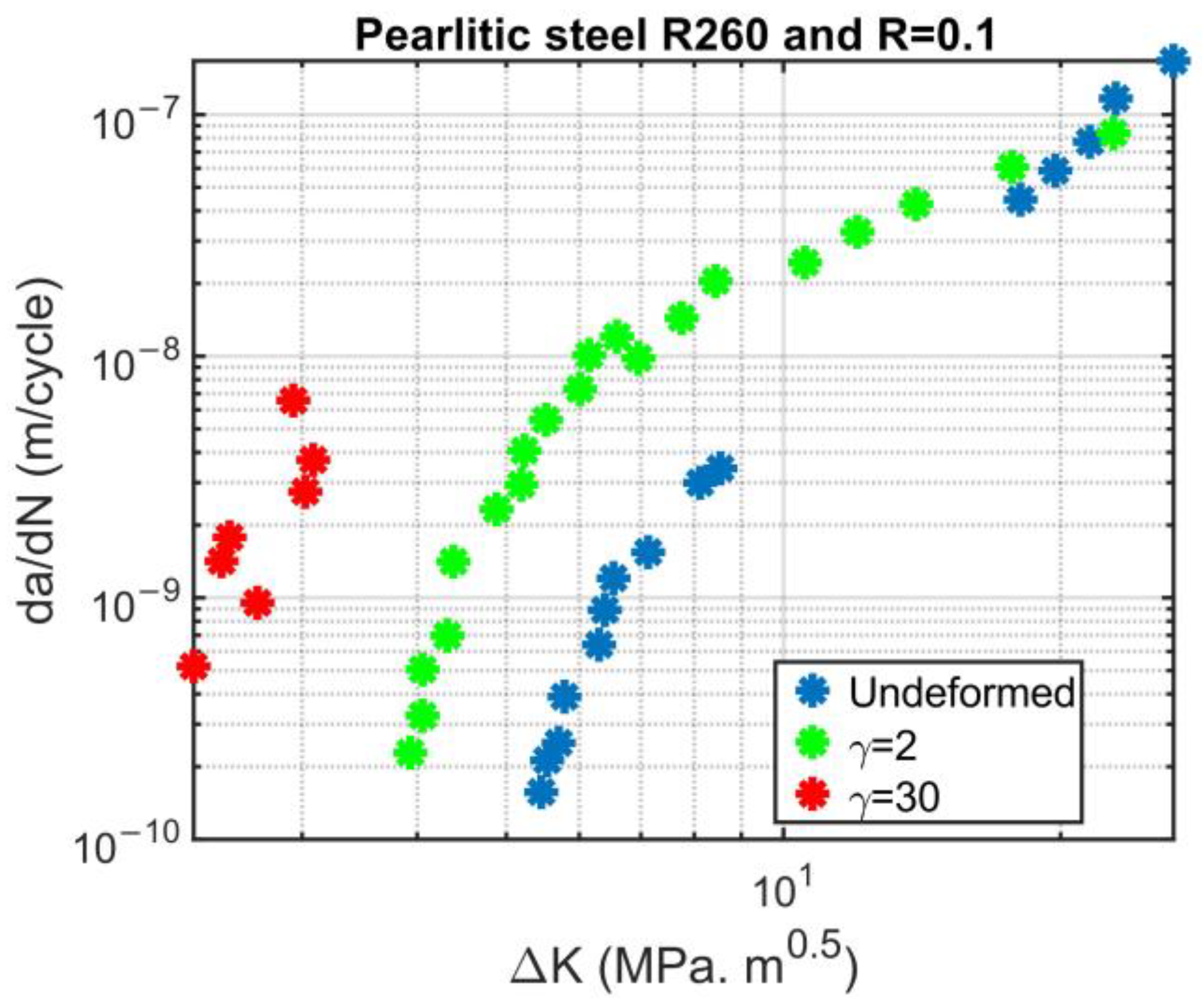
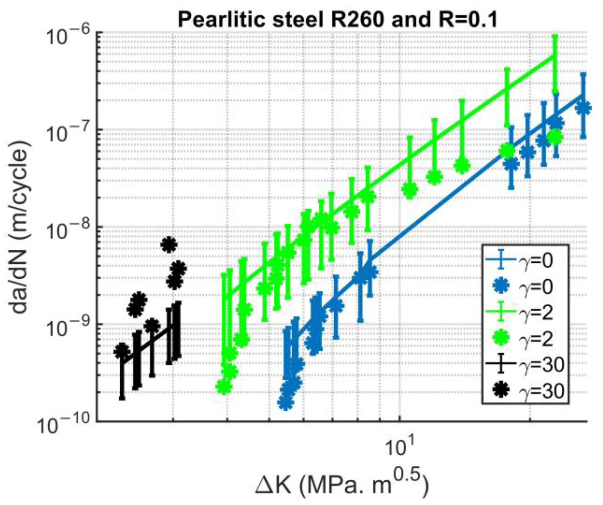
The result of fatigue crack simulation and the experimental results for different deformation states are shown in
Figure 12. To generate
Figure 12, all four repetitions of three deformation state meshes needed to be run, and the combined result with the error bar was calculated and is shown in this figure. It is worth emphasizing again that these results are parameterized for the undeformed state and validated for both deformed and severely deformed states. Measurement errors or unaccounted parameters may cause a difference in the FCG rate for the severely deformed state between simulation and experiments. However, the results are sufficiently acceptable because the same damage law and constant parameters were used throughout the analysis. The model parameters used in the simulations can be seen in
Appendix A.
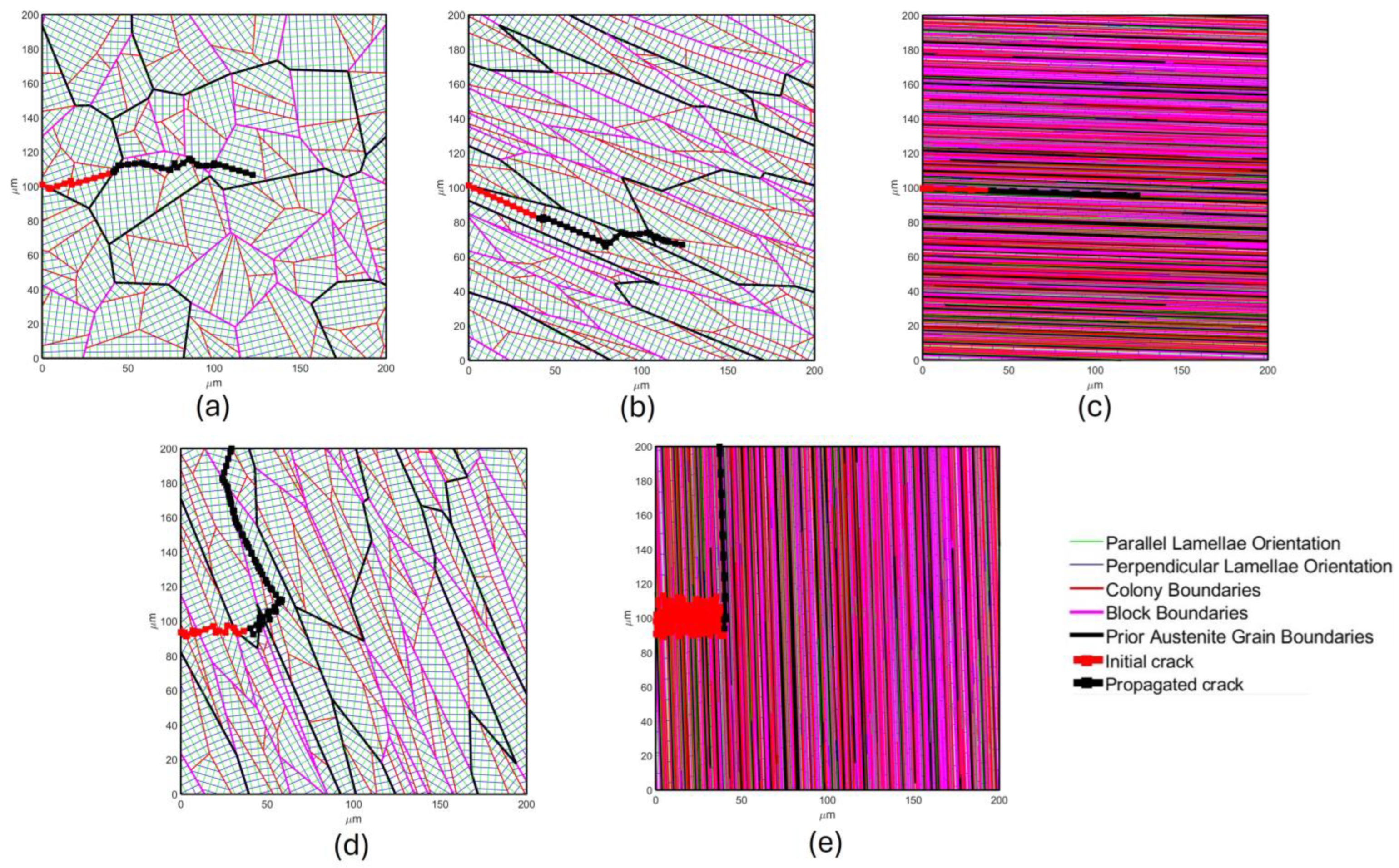
Another interesting set of results that can be concluded from the DEM simulation is the crack paths for each deformation state. The crack path for the meshes is shown in
Figure 13. The results show that, when the deformation goes higher, the crack path tends to be smoother, which is in agreement with the observation reported by Leitner et al. [
18,
19,
40].
As shown in
Figure 13, the degree of deformation and its orientation significantly influence the crack trajectory. The model predicts that cracks primarily grow along the interface between cementite and ferrite lamellae when there are no geometrical constraints. This prediction is consistent with the findings of Leitner et al. [
40], which state that, in pearlitic steels, cracks predominantly propagate along the interface between the ferritic and carbon-rich (previously cementite) phase. Crack tortuosity is a parameter that can describe how twisted or curved a crack path is compared with a straight-line crack path. The crack tortuosity parameter measures the deviation of a crack path from a perfectly straight path. It is defined as the ratio of the actual path to the straight-line distance between the crack’s beginning and end (in this case, the distance along the x-coordinate).
Figure 14 shows the crack tortuosity for different deformation states simulated by DEM. It is important to note that tortuosity was not calculated for the severely deformed state in the T–A orientation because of the extremely short crack length along the x-coordinate; this value would be much higher than others. The higher values of crack tortuosity may explain the crack growth rate anisotropy in pearlitic rail steel material. For a slower orientation, e.g., T–A orientation, the crack should encounter more deviation in its path when it needs to reach a specific length.
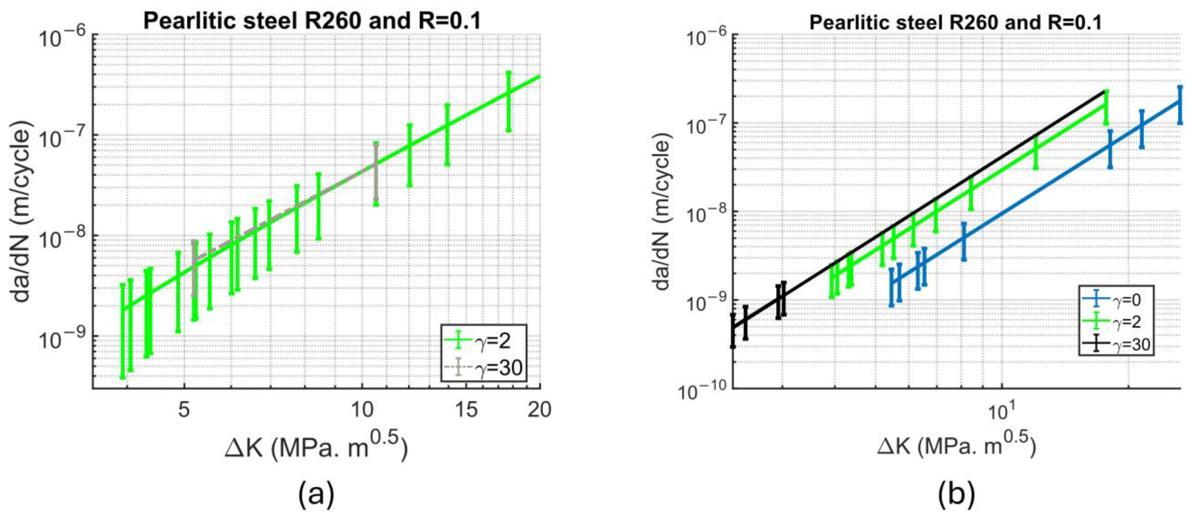
To investigate the influence of the different deformation states on fatigue resistance, the crack evolution of SPD and moderately deformed meshes under similar stress intensity factor ranges were simulated. The results shown in
Figure 15a were obtained with the previously adjusted values of
and
.
Figure 15a shows that the differences in the FCG rate between the SPD and moderately deformed conditions were minimal. This means that the increment in the FCG rate predicted by the model started already at a moderate deformation level of
(see comparison with undeformed state in
Figure 12). Furthermore, simulations were performed using the same values of
and
to isolate the effect of mesh deformation on FCG (see
Figure 15b). The results show that the FCG rate increased mainly due to the re-orientation of microstructural components occurring already at moderate deformation of
. Finally, it can be concluded that the strain hardening that modified the yield strength did not considerably affect the FCG rate.


 ,
, 
