Abstract
The looper-tension control is a crucial aspect of a hot strip finishing mill. It involves a highly nonlinear system with strong states coupling and uncertainty, and the performance directly impacts the thickness deviation, which is the most critical product index. From the system dynamics, it is known that tension is highly sensitive to the strip velocity variation, which is typically unmeasurable. Instead, it needs to be calculated through work roll speed and strip slip which contains uncertainties, negatively affecting tension control performance. First, a feedback linearization-based proportional–integral (PI) controller design approach is proposed for the hot rolling looper-tension system. Second, to reduce the impact of speed uncertainties and enhance thickness response, an adaptive PI controller is introduced. Validation was conducted by numerical simulations; the result indicates that an adaptive PI controller reduces the magnitude of thickness variation and shortens the duration of its impact, verifying the consistency between theoretical derivation. The proposed control method effectively addresses the impact of uncertainties encountered in real-world applications. Additionally, it simplifies control parameter adjustment in practical use, reduces testing time, and improves product quality.
1. Introduction
Thickness precision is one of the most important quality indexes in the hot strip mill finishing rolling process, and the automatic gauge control (AGC) is the most direct and effective method for adjusting thickness. The hot rolling process is highly complex, with multiple interacting factors. Several studies [1,2,3,4] have highlighted tension as a key factor influencing strip thickness. A looper installed at the inter-stand, which is the major equipment used to control the strip tension between the two stands.
In these decays, various looper-tension control schemes have been proposed, such as conventional PI control methods [5,6], multivariable control methods [7], and inverse linear quadratic (ILQ) control [8,9], which have been studied and wildly used in the industry. However, these conventional looper tension control systems may suddenly become unstable due to the change in the characteristics of rolled material and the slip between roll and strip while rolling. To overcome this problem, the robust control [10,11] method had been proposed. However, there exists a main problem of slow response of these conventional robust controllers.
Moreover, due to the nonlinear nature of the system and the presence of disturbances, the working situation of these control methods is limited. To overcome this, several nonlinear control schemes have been proposed. The recursive nonlinear techniques for the looper tension system is shown in [12]. Ref. [13] uses the sliding-mode control (SMC) approach to compensate for looper friction phenomena. However, the parameter uncertainties of these control schemes could affect the robustness and control performance dramatically, and the multivariable controller tunning is a hard task due to lacking transparent structure [14].
Adaptive control has been extensively utilized to mitigate parameter uncertainties and external disturbances, thereby enhancing system performance. Ref. [15] investigated an adaptive receding horizon control approach to address parameter variations in looper-tension control. Additionally, adaptive controllers have been employed to attenuate inevitable friction effects and external disturbances [2]. Ref. [16] identified time-variant slip as the primary cause of mass flow disturbances. Studies such as [12,17] also highlighted the significant impact of speed disturbances on system performance and demonstrated the effectiveness of adaptive feedback controllers in enhancing control outcomes.
Although adaptive control methods have shown promising results, existing studies often lack a comprehensive methodology for selecting robust control gains and fail to explicitly address the influence of uncertainties on thickness deviation. This motivates the present study to design a looper-tension nonlinear controller that accounts for uncertainties and optimizes robust control performance using the linear matrix inequalities (LMIs) technique.
To address the inherent nonlinearity of the system, state feedback linearization is employed, as in [18]. The core concept of this technique is to cancel the system’s nonlinearities, thereby enabling the achievement of desired linear dynamics for control. Nevertheless, because system parameters are often difficult to match precisely with their true values, it is crucial to design a robust controller that considers these uncertainties. The LMIs technique has been widely used for robust controller design and analysis [19]. In [20], the controller of an nonlinear heating device with uncertainties and disturbances is designed via LMIs. Meeting the required time domain specifications is also an important issue in control design [21]. Through LMIs technique, optimization design can be performed for the desired time domain specifications. In addition, to enhance control performance, an adaptive controller is proposed specifically for forward/backward slip uncertainty, which is the main source of tension variation.
The specific contributions are summarized as follows: (1) In system representation, we represent the looper-tension system using error dynamics, explicitly incorporating slip uncertainty as the primary uncertainty factor. (2) A robust looper-tension controller is developed using feedback linearization and an LMIs-based optimization approach to ensure stability and satisfy time-domain specifications. Building on this robust framework, an adaptive PI controller is introduced to further attenuate tension variations caused by forward/backward slip uncertainty, resulting in progressive improvements in tracking performance and robustness. (3) Numerical simulations demonstrate that the proposed control strategy effectively achieves the desired control objective. Compared to the PI controller, the adaptive PI controller reduces thickness variation from 0.0233 mm to 0.0168 mm and decreases convergence time from 7 s to 3.563 s (a 49% improvement). This confirms that the proposed control method can significantly enhance the quality of the steel strip.
2. Process Model
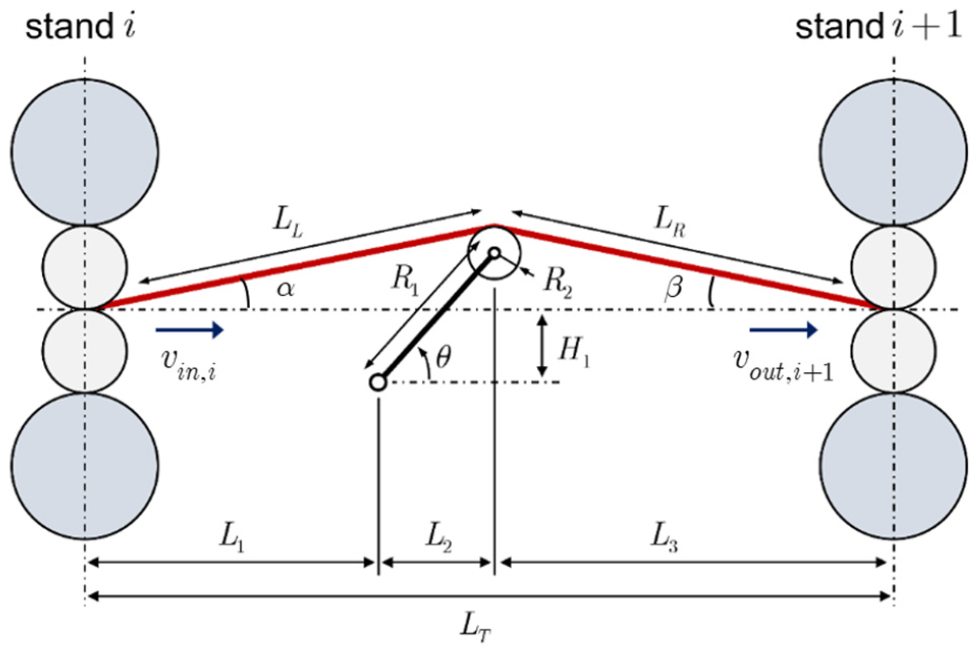
Hot rolling is a highly complex system, various factors, such as thickness, rolling force, and tension, exhibit mutual coupling effects. To simplify control challenges, most steel mills implement a control framework that separates thickness and tension control. This study focuses primarily on looper-tension control, an overview of the tension and looper model is provided in detail, which is used to synthesize the controllers. The looper and inter-stand geometry is given in Figure 1. Moreover, variables such as thickness and rolling force can be calculated utilizing rolling mechanism models, BISRA gauge-meter, and Sims formula [22], thereby deriving the influence of tension on thickness.
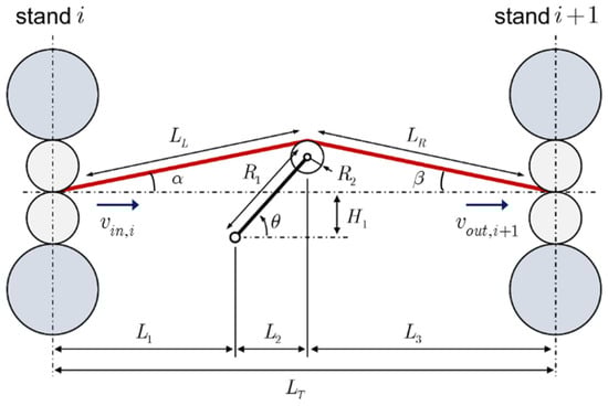
Figure 1.
Physical model of two stands and looper.
2.1. Looper-Tension Dynamics
The inter-stand strip tension described here is close to [1,18], which is defined by Young’s modulus of the strip and the Hooke’s law:
where is the looper angel; is the distance between two stands; is the geometric length between stands (the geometric variables are shown in Figure 1); and is the mass flow difference. is rather small compared to . As a result, (1) can be approximated by:
The geometric length between stands is shown as follows:
And the mass flow difference in the strip between stands can be evaluated as follows:
is the strip speed leaving stand i, which depends on the speed of the work rolls , its radius , and the forward slip
while is the strip entering stand i + 1. Similarly, it is related to the work roll speed and the backward slip
Forward and backward slip are influenced by tension, thickness, and rolling force, as described in [23]. In this model, the forward slip is mainly related to the following variables: work roll speed , entry thickness , exit thickness , forward tension , backward tension .
Based on (2), the derivative of inter-stand strip tension between the ith stand and the i + 1th stand can be obtained as follows:
only depends on the looper angle , according to the chain rules:
By substituting (7), (8), and (11) into (10), the dynamic model of strip tension can be expressed as follows:
For looper dynamics, the looper angle is determined as follows:
where is the looper angular velocity, based on Newton’s second law of motion, the equation of the looper torque can be derived as
where is the viscous damping coefficient, is the hydraulic torque applied to the looper, and is the load torque of the looper shown as
The load torque is combined with the inter-stand tension, strip weight, looper arm weight, and strip bending force [1,18], respectively. The load torque due to strip tension is
The torque of the strip weight with steel density is
The torque induced by the looper arm is
The torque of strip bending force is
where is the strip width, is the strip thickness, is density of the strip, is gravitational constant, is the looper weight, is the distance from the pivot to the center of mass of the looper, and the other variables are shown in Figure 1.
The dynamics of the entire system can be rewritten as state equations
2.2. Problem Statement and Controller Design
System uncertainty is one of the main reasons for the degradation in control performance. To improve system stability and performance, a feedback linearization-based PI control approach is first proposed, and the characteristics of the closed-loop system can be adjusted through pole placement to enhance system stability and meet desired time domain specifications. Then, an adaptive control term is introduced to estimate uncertainties, further improving control performance.
The control goal is to design control signals that both the looper angle and strip tension can track the given reference, respectively. The model is represented by the error from the reference inputs:
Differentiating (21) with respect to time, the error dynamics equations are as follows:
For the looper and tension system, several sources of disturbances and unmodeled dynamics should be considered. In the tension subsystem, both forward and backward slip are difficult to measure accurately and are highly sensitive to the tension dynamics [18]. Set-up mismatches and mass flow variations from the AGC system can also affect the tension. In the looper subsystem, the torque is calculated via an empirical formula, which introduces inherent uncertainty. Moreover, previous studies have identified speed perturbation as the primary source of disturbance [12,18]. Given that slip is directly related to speed and is inherently difficult to measure accurately, the uncertainty in slip calculation is regarded as the primary source of system uncertainty in this study. Accordingly, the forward/backward slips are further divided into known and unknown components and can be rewritten as
in which the known parameters are and , and the unknown uncertainty values are and . Substituting (23) into (22) yields the dynamic equation for the looper-tension tracking error with parameter uncertainty, the state-space representation is as follows:
where , the error dynamic can also represent in vector form as
The terms represent nonlinear matrices that can be eliminated through feedback linearization, allowing the system dynamics to be transformed into a more manageable linear form. The term represents a nonlinear matrix containing uncertainties, which cannot be completely canceled and must be addressed using robust or adaptive control techniques.
Note that the upstream speed is typically selected as the control input, while the downstream speed is treated as a constant to achieve the desired speed differential for control purposes.
According to the error dynamic (25), the feedback linearization-based PI control law is designed as
in which can be divided into the nominal term and the PI term as follows:
The principle behind feedback linearization is to cancel the known nonlinearities in the system dynamics by introducing a compensatory nominal control action. This process transforms the original nonlinear system into an equivalent linear one, allowing conventional linear control techniques, such as the PI controller, to be applied more effectively. In our design, the nominal term , shown as (28), is specifically constructed to eliminate the known part of the dynamic equation.
and the PI term is the typical control law
To analyze the stability, define an extended state as follows:
The extended close-loop system can be described by
where , and the system matrix is described as
Then, the PI control law can be described as vector form
where is the control gain matrix with the following specific form
By substituting (26) into (31), it gives
where is the close-loop matrix which is composed of two subsystems and , is the uncertainty matrix, is a nonlinear function, and is the uncertainty with a nonlinear terms matrix. Note that , , and originated from slip uncertainties, representing the variations and nonlinear effects. The detailed structures are as follows:
Examining the structure of , we observe that since the uncertainty matrices share the same dimension, it can be represented as a one-dimensional uncertainty matrix:
in which
To solve the robust control gain under the uncertainties, the uncertainty matrix can be expressed as
Assuming the uncertainty matrix is bounded by a norm bound, and a factorization can be employed to reduce the conservativeness of this assumption, shown as
and
where is the known positive constant and the value can be determined through system identification or experimental experience.
Since the looper can only vary within a fixed range, it is reasonable to assume
Additionally, the uncertainty in the backward slip ratio is assumed to remain within a defined range
Thus, the existence of (39) is constrained within a specific bound range
where
Consequently, the uncertainty matrix is constrained to a specific bounded region as follows:
in which .
Finally, the error dynamic can be represented as
Equation (48) describes how the PI controller affects error dynamics and how uncertainties influence system behavior. Consequently, an adaptive law is formulated to estimate and compensate for these uncertainties, thereby enhancing system performance. To this aim, the error dynamics equation is separated into known and unknown parts, shown as
where is the matrix combined with , and is the uncertainty matrix, shown as
Different from the PI control law (26), the adaptive PI control law is designed as
Similar to (27), can be divided into the nominal term , the PI term , and the adaptive law as follows:
where the structure of nominal term and the PI term are the same as (28) and (29). The adaptive law is specifically designed to estimate and compensate for parameter uncertainties. Assuming the parameters in are known and measurable, the adaptive law can be designed as
where is the estimated parameter matrix given by
The purpose of designing the adaptive PI controller is to enhance tracking performance in the presence of parameter uncertainties. If the estimated uncertainties are more accurate, the system will be less affected by those uncertainties. This is especially evident for tension, as it is highly sensitive to speed. To estimate these parameter uncertainties, the parameter estimation errors are defined as
Apply the control law by (51) and the error dynamics become
2.3. LMI-Based Robust Stability Analysis and Controller Gain Calculation
In [24,25], the robust pole placement within LMI technique not only ensures system stability but also achieves robust performance. For the hot strip rolling looper-tension system, the system under consideration consists of two subsystems, each with unique dynamic requirements. First, we propose LMIs for computing the optimal PI controller gains that ensure stability and meet the required performance specifications, as follows:
Theorem 1.
For the closed-loop nonlinear system (48), the robust control gain can be obtained by considering the following constrained problem, represented by the LMIs: given and
where , and are the decision variable. The control gain of the PI term control law can be obtained with the constraints. Moreover, the tracking error is ultimately bounded by
for .
Proof of Theorem 1.
Consider the system tracking error dynamics, select the Lyapunov candidate function
To ensure robust performance in the presence of model uncertainty, we require that the Lyapunov inequality is satisfied as follows:
where is a diagonal matrix, shown as (62), to ensure the desired convergence rate.
It also restricts the eigenvalues of the subsystems close-loop matrix and constrained within and , respectively. It is evident that (61) is achieved if the following inequality is guaranteed
Based on Cauchy–Schwarz inequality and the upper bond assumptions by (41) and (42), (63) is guaranteed if the inequality is represented as
where , , and the rest of the variables are defined as
Based on Schur’s Complement, Equation (64) can be further translated into the standard LMI form as follows:
Consequently, if the corresponding LMI is feasible, robust stability is guaranteed. Since it is assumed that the system is affected solely by slip uncertainties, it can be observed from (37) that and influence only the tension subsystem. As proven in Appendix A, the term eventually converges to zero when . Therefore, based on (66) and (47), (61) can be guaranteed and the derivative of the Lyapunov function along the error trajectory is given by:
which implies when , where
The result shows the system’s tracking error trajectory is confined in a disk of radius in the phase plane, then the result of (59) is proofed. □
Remark 1.
The stability of the error dynamics in the presence of uncertainties is ensured through ultimate boundedness, with the bound determined by (68). Additionally, the trajectory tracking accuracy is influenced by the magnitude of , which is directly affected by the uncertainty . Through the design of the parameter , the proximity of the closed-loop system eigenvalues to the imaginary axis is adjusted, which indirectly influences the magnitude of . Typically, as increase, becomes larger, enabling a reduction in .
Remark 2.
The selection of controller gains in addition to providing system stability and robustness, is also crucial for the performance of transient response. As is well known, the transient response of a system is closely related to the location of its poles. Taking the standard second-order system step response as an example, the poles can be represented in the complex plane by the undamped natural frequency , the damping ratio , and the damped natural frequency . In the control design, consider two important time domain specifications in general engineering practice: the settling time and the overshoot (related to damping ratio ).
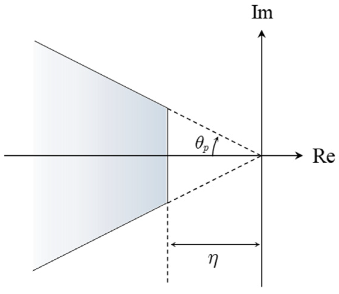
To satisfy these two specified specifications and achieve an acceptable transient response, the designed closed-loop poles will be placed within the sector region shown in Figure 2. However, systems typically involve certain uncertainties. When the model is subjected to uncertainties, it is important to ensure that the poles remain within the specified region. Such robustness issues can often be addressed through pole placement within the LMI region [25].
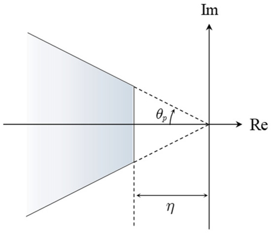
Figure 2.
Conic region in the phase plane where the closed loop poles are constrained.
Based on the region specified in Figure 2 constraints are imposed that involve vertical strips and a conic sector. The LMI (57) guarantees the real parts of the poles of each system are smaller than and , satisfying the region constraint of the left half of the vertical strip in Figure 2. This ensures that the closed-loop system with poles in this region has the maximum settling time and . On the other hand, the conic sector restricts the minimum damping ratio of the closed-loop system. Referring to [25], the formulation for the LMI of conic sector constrain is
It can also be written as
where
By taking the intersection of the constraints defined in (57) and (70), the closed-loop poles are placed within the region specified in Figure 2, enabling the system to satisfy specific transient performance requirements.
As mentioned earlier, the choice of directly affects the convergence of the entire system. Increasing implies placing the closed-loop poles further away from the imaginary axis. While this can enhance the convergence performance of the system, it can also lead to what is known as high-gain control. High-gain control is unfavorable for practical control implementation, as it can easily result in control saturation or increased costs.
Therefore, in order to avoid high gain control as much as possible under the specified , minimize the size of the control gain matrix as an objective, which can be performed by considering the following inequality:
where the variable stands for a norm bound of gain , which should be minimized. The problem of nonlinear matrix inequalities can also be expressed as LMI:
By definition
, to guarantee that the minimization of
is equivalent to the minimization of the control gain
, the condition
is further imposed into the LMIs framework.
Therefore, the LMI condition for minimizing the control gain can be written as
As a result, performance enhancement can be formulated as a synthetic minimization problem along with the LMIs feasibility problem of the control design. Then, the optimal control gain can be calculated.
Theorem 2.
For the error dynamics (56) with the assumption that the system parameter is time-invariant, and the main uncertainties come from the slip ratios. By applying the proposed adaptive PI controller (51) with the designed adaptive law (75), the stability and convergence rate can be ensured.
where is an adaptive gain. Given that the uncertainties are constrained within a small range, the estimated value of is expected to remain relatively small. Consequently, setting and can be considered a valid and reasonable assumption.
Proof of Theorem 2.
Consider the Lyapunov function candidate of the quadratic form:
where . Taking the time derivative on (76) yields
Based on the parameter time-invariant assumption:
substituting (78) and the adaptive law (75) into (77) gives
If the following inequality
holds, then (79) can be derived as
It can be seen that as long as . As a result, the stability of the system can be ensured. □
Remark 3.
For adaptive controller gain design, the Lyapunov inequality is desired to be
It is evident that (82) is achieved if the following inequality is guaranteed:
The optimal PI adaptive controller gain can be obtained by solving (83) and the LMI condition (74). By observing the LMI constraints, the PI controller imposes more stringent conditions. This also implies that the optimal gain values obtained for the PI controller from (57) will satisfy the LMI conditions for the adaptive controller in (85) as well.
Furthermore, to explicitly clarify the distinction between the nominal PI controller and the adaptive PI controller, we emphasize their different roles in the control strategy. The nominal PI controller is designed using feedback linearization to compensate for known system dynamics, ensuring robustness against modeled uncertainties. However, it does not account for unknown disturbances, limiting its ability to handle unmodeled uncertainties effectively. In contrast, the adaptive PI controller extends this framework by incorporating an additional term in (53) within the control law. This adaptive mechanism enables real-time adjustment of control parameters, effectively mitigating the impact of slip uncertainty. From (67) and (81), it can be seen that the adaptive controller enables the error to converge to zero, whereas the PI controller can only reduce the error to a bounded region. This distinction highlights the advantage of the adaptive approach in achieving greater control precision and robustness, particularly in the presence of parameter uncertainties.
Remark 4.
While using large adaptive gains can accelerate the estimation convergence, it often leads to noticeable oscillations in the estimation process and increases control effort. Conversely, small adaptive gains produce smoother but slower transient estimations. During the steel strip production process, severe oscillations can lead to various issues; therefore, high adaptive gains are typically avoided.
3. Numerical Simulations
The proposed PI and adaptive PI controllers were compared using MATLAB/Simulink (R2021b) software. The error dynamics of the system are the basis for the Simulink model developed with numerical solver Runge–Kutta 4 and a time resolution of 0.001 s. The simulation is based on the Looper 6 in a seven-stand hot strip finishing mill, where the looper reference angle is , the strip tension reference is MPa, and the upper bound uncertainty matrix was set as .
To ensure production stability, the rolling mill speed and looper involve significant inertia, resulting in a typically slower transient response in control relative to equipment specifications. Typically, the looper can be adjusted more quickly than the rolling mill speed. A fast response helps effectively prevent excessive stretching or slackening of the steel strip, ensuring continuity in the production process and maintaining product quality. Therefore, the system time domain specifications are assumed as follows: a looper settling time , a work roll speed settling time , and a damping ratio for both systems . Accordingly, the closed-loop poles are constrained to lie within a sector region, defined by , and, . In the design of the PI controller, it is essential to simultaneously satisfy both robustness and expected time specifications. The control gains are obtained through optimization based on LMIs. In this study, we utilize the MATLAB LMI Toolbox (R2021b) to perform offline computations for control gain determination. This approach ensures that the optimal gain solutions are precomputed and readily applicable to the control system, significantly enhancing the feasibility of practical implementation. The optimal gain solutions are as follows:
with the relationship of , the PI controller gain matrix is designed as
All eigenvalues of the close-loop matrix are verified to meet the designed constrain region, where and . Thus, the feedback linearization-based PI control law (26) can be applied to the looper-tension system. To compare the difference in control performance between the PI and adaptive PI controller, the control gains are set to be the same for both. The adaptive gain of (75) is given as , and the selection of is the same as (84). Finally, the adaptive PI control law (51) can be implemented. The control parameters are shown in Table 1 and the control targets and system parameters are shown in Table 2.

Table 1.
Control parameters.
Table 2.
Control target and system parameters.
To show the validity of the proposed algorithm, we illustrate the numerical example comparison. A tandem rolling process environment is established, in which the rolling force is calculated by a Sims model, the thickness response is based on the AGC with Smith predictor [26], and the slip ratio is obtained through (9) where the uncertainties are given as
The entry thickness is 3.6363 mm, with a target exit thickness of 3.0346 mm, and the uncertainties were applied at t = 3. After the thickness reached a steady state, to demonstrate the impact of uncertainty on thickness. The comparison of simulation results between PI and adaptive PI control is shown in Figure 3, and the control inputs are depicted in Figure 4. The tracking error of the looper-tension system and the strip thickness are shown in Figure 5 and Figure 6, respectively.
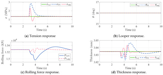
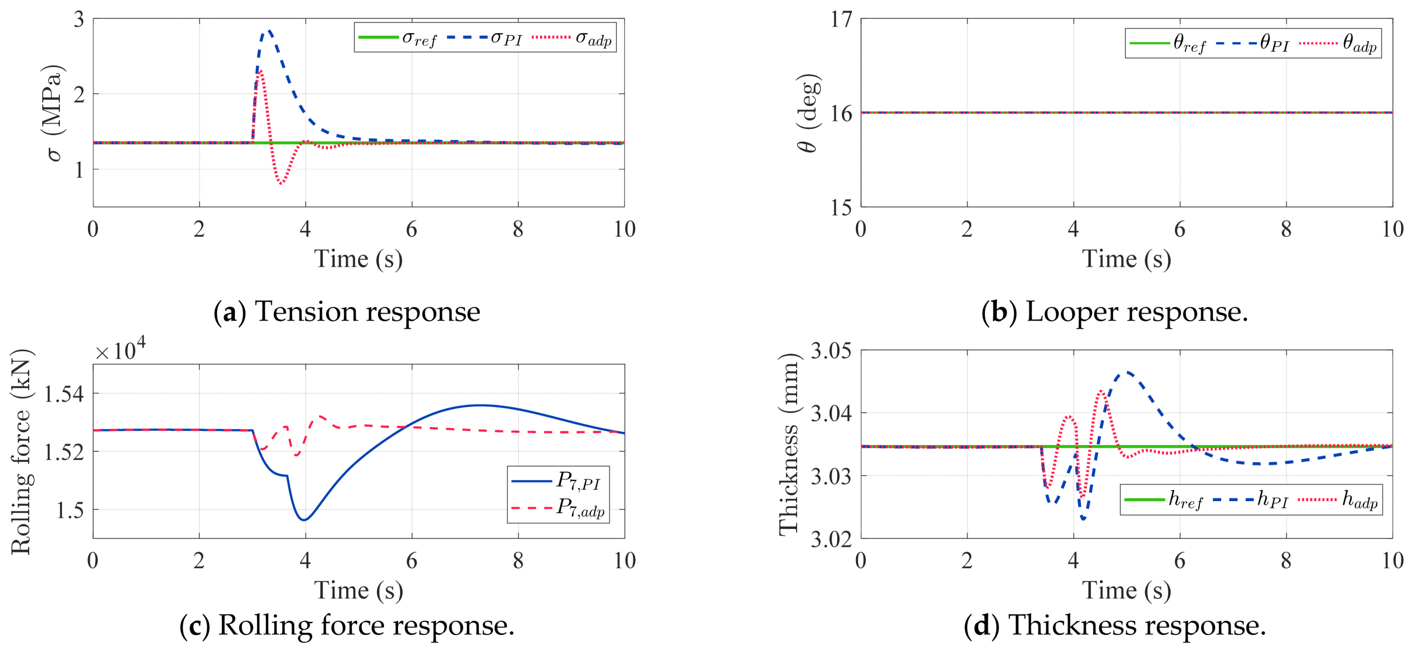
Figure 3.
Comparison of simulation results between PI and adaptive PI control.
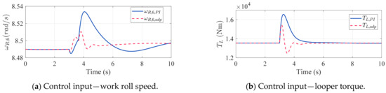
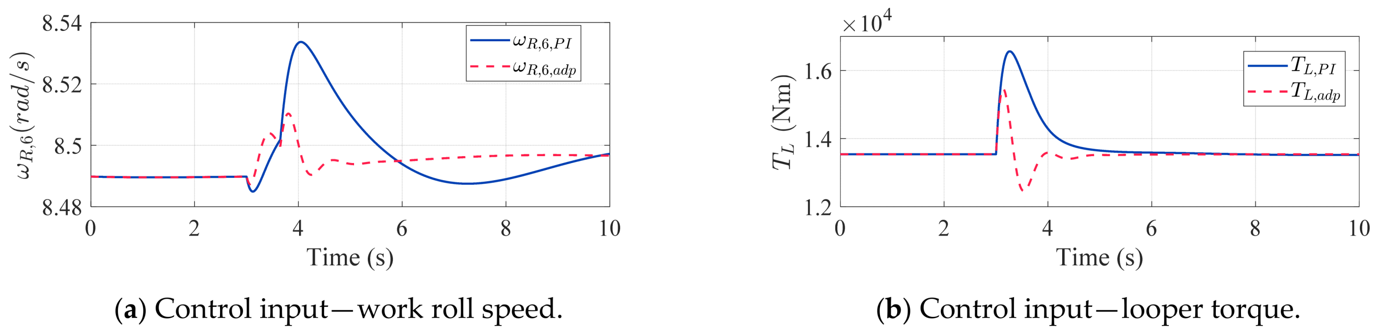
Figure 4.
Control input comparison.
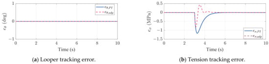
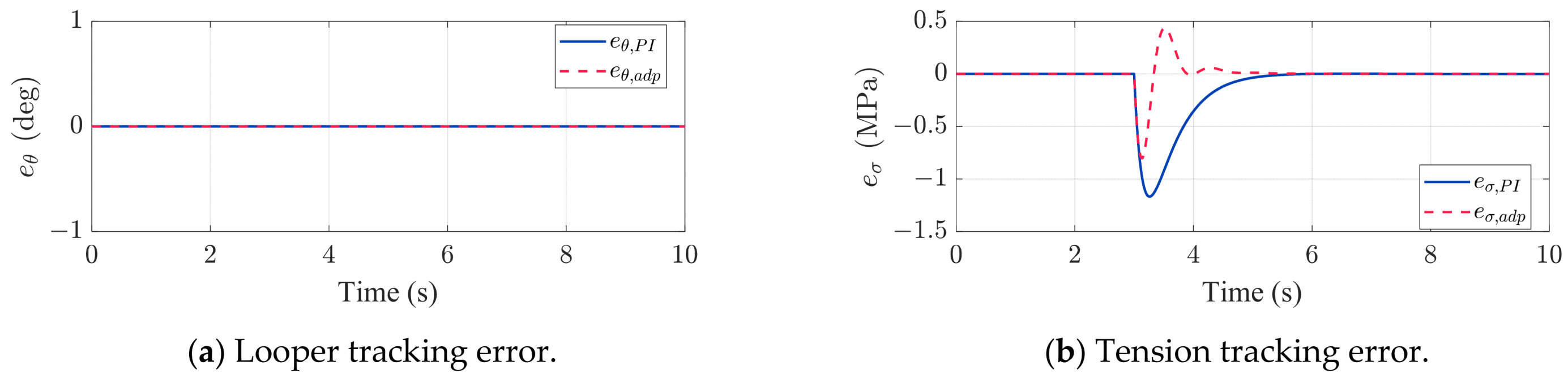
Figure 5.
Tracking error comparison of PI and adaptive PI control.
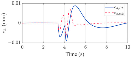
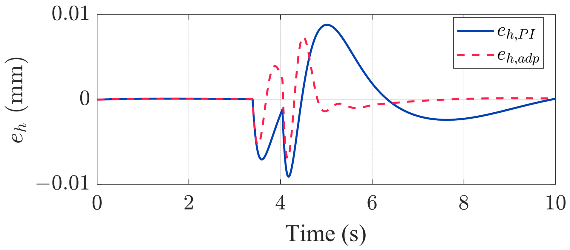
Figure 6.
Thickness error comparison.
Under PI control, the result shows the tension response is highly sensitive to slip uncertainties, resulting in substantial fluctuations, as shown in Figure 3a. Through adjusting the upstream rolling speed, Figure 4a, tension is controlled towards the target value, ultimately achieving stability. In the looper part, due to the use of feedback linearization and the assumption of minimal deviation between calculated and actual values, the output effectively maintains the angle at the desired position, as seen in Figure 3b. The thickness response is influenced by various factors and control mechanisms, such as rolling force and AGC, with simulation results shown in Figure 3d. The variation in thickness originates from changes in rolling force (see Figure 3c), which is influenced by the tension response. This illustrates the impact of slip uncertainties on strip thickness deviation. Tracking errors of the looper-tension system are shown in Figure 5, and the thickness error is depicted in Figure 6. It is evident that control error ultimately converges with PI controller, aligning with the theoretical derivation.
In the adaptive PI control framework, Figure 3a demonstrates that the tension converges more rapidly through the adaptive law, with a notably reduced magnitude of control input adjustments, as shown in Figure 4. This outcome significantly reduces the rolling force variation, as illustrated in Figure 3c, allowing the thickness to converge to the target more swiftly, as shown in Figure 3d. It implies that if uncertainties can be quickly estimated and mitigated by the adaptive PI controller, the thickness variation can be significantly reduced.
Figure 5 demonstrates that the tracking error will converge with an accelerated convergence rate, consistent with theoretical derivation. Figure 6 indicates that due to the reduction in both tension and rolling force variations, thickness variation not only decreases but also achieves a faster convergence rate. Table 3 presents a comparative analysis of tracking error performance. The Adaptive PI reduced the thickness variation from 0.0233 mm to 0.0168 mm, corresponding to an improvement of 27.82%, and decreased the convergence time from 7 s to 3.563 s (a 49.10% improvement). For tension control, the convergence time was reduced from 4.669 s to 1.886 s, representing a 59.61% improvement. These findings demonstrate that the Adaptive PI controller markedly improves both the dynamic response and accuracy of the control system. This improvement enhances the process stability and the quality of the final product.
Table 3.
Tracking error performance comparison.
4. Conclusions
To address the nonlinearities in hot rolling control and optimize control gains selection across different system, an innovative looper and tension control approach based on the LMI optimization was investigated. The feedback linearization technique is used to cope with nonlinearities on the system. Considering the forward/backward slip uncertainties, which are sensitive to tension, the optimal PI controller with robust stability and desired performance was formulated via LMIs. Furthermore, an adaptive PI control scheme was proposed and implemented to mitigate the impact of slip uncertainties and improve the transient response. The proposed method not only enables rapid determination of robust and optimal control gains but also improves the transient response with the impact of uncertainties.
To address the nonlinearities in hot rolling control and optimize control gain selection across different systems, an innovative looper and tension control approach based on LMI optimization was investigated. The feedback linearization technique was employed to manage the system nonlinearities. Considering the forward/backward slip uncertainties that are sensitive to tension, an optimal PI controller ensuring robust stability and desired performance was formulated via LMIs. Furthermore, an adaptive PI control scheme was proposed and implemented to mitigate the impact of slip uncertainties and improve transient response.
The proposed method enables rapid determination of robust, optimal control gains and improves transient response under uncertainties. Moreover, this method employs only PI control and adaptive control, which makes it easier to implement in industrial environments (e.g., PLC systems). Despite its promising performance in simulation, several limitations remain. Potential implementation challenges include additional model uncertainties or disturbances, as well as measurement signal noise encountered during practical applications. If we cannot ascertain the form of the uncertainties or disturbances, the performance of the adaptive control will be limited. Moreover, experimental validation is a valuable future direction to confirm the real-world applicability of the proposed approach.
Author Contributions
Conceptualization, C.-C.P.; methodology, Y.-C.H.; software, Y.-C.H.; validation, Y.-C.H.; formal analysis, Y.-C.H. and C.-C.P.; investigation, Y.-C.H.; resources, C.-C.P.; data curation, Y.-C.H.; writing—original draft preparation, Y.-C.H.; writing—review and editing, C.-C.P.; visualization, Y.-C.H.; supervision, C.-C.P.; project administration, C.-C.P.; funding acquisition, C.-C.P. All authors have read and agreed to the published version of the manuscript.
Funding
This research was funded by the China Steel Corporation, R.O.C, under RE112007.
Data Availability Statement
Data are available upon reasonable request.
Conflicts of Interest
Author Yu-Chan Huang was employed by the company China Steel Corporation. The remaining authors declare that the research was conducted in the absence of any commercial or financial relationships that could be construed as a potential conflict of interest.
Appendix A
Tracking Error Derivation
The system tracking error dynamics can be expressed as two subsystems
where
The Lyapunov candidate Function (60) can be described with the subsystems:
where and .
For subsystem , the time derivative of is
To ensure the robust performance in the presence of model uncertainty shown in (63), the Lyapunov inequality is desired to be
If the LMI (68) is feasible, (A6) can be guaranteed. Thus, the subsystem is asymptotically stable, which implies when .
For subsystem , the time derivative of is
With the same concept of (A5), the Lyapunov inequality is desired to be
If the LMI (68) is feasible, (A9) can be guaranteed.
The derivative of the Lyapunov function along error is bounded using the Cauchy–Schwarz inequality shown as follows
which implies when , where
Since when , the bounded tracking error of becomes
The above proves that the influence of the nonlinear matrix on the tracking error approaches zero as .
References
- Yin, F. Discrete model predictive control scheme for an integrated gauge-looper control system in a tandem hot strip mill. IEEE Access 2020, 8, 73972–73985. [Google Scholar] [CrossRef]
- Xiao-hong, J.; Shao, L.-p.; Peng, Y. Adaptive coordinated control for hot strip finishing mills. J. Iron Steel Res. Int. 2011, 18, 36–43. [Google Scholar] [CrossRef]
- Müller, M.; Prinz, K.; Steinboeck, A.; Schausberger, F.; Kugi, A. Adaptive feedforward thickness control in hot strip rolling with oil lubrication. Control Eng. Pract. 2020, 103, 104584. [Google Scholar] [CrossRef]
- Prinz, K.; Steinboeck, A.; Kugi, A. Optimization-based feedforward control of the strip thickness profile in hot strip rolling. J. Process Control 2018, 64, 100–111. [Google Scholar] [CrossRef]
- Choi, I.; Rossiter, J.; Fleming, P. Looper and tension control in hot rolling mills: A survey. J. Process Control 2007, 17, 509–521. [Google Scholar] [CrossRef]
- Gaber, A.; Elnaggar, M.; Fattah, H.A. Looper and tension control in hot strip finishing mills based on different control approaches. J. Eng. Appl. Sci. 2022, 69, 100. [Google Scholar] [CrossRef]
- Kotera, Y.; Watanabe, F. Multivariable control of hot strip mill looper. IFAC Proc. Vol. 1981, 14, 2471–2476. [Google Scholar] [CrossRef]
- Ji, Y.; Yuan, H.; Song, L.; Li, H.; Peng, W.; Sun, J. Coordinate control of strip thickness-crown-tension based on inverse linear quadratic in tandem hot rolling mill. Int. J. Adv. Manuf. Technol. 2022, 118, 1213–1226. [Google Scholar] [CrossRef]
- Yuan, H.; Li, X.; Wang, X.; Ji, Y. A looper-thickness coordinated control strategy based on ILQ theory and GA-BP neural network. Int. J. Adv. Manuf. Technol. 2023, 127, 4845–4860. [Google Scholar] [CrossRef]
- Hearns, G.; Grimble, M.J. Robust multivariable control for hot strip mills. ISIJ Int. 2000, 40, 995–1002. [Google Scholar] [CrossRef]
- Imanari, H.; Morimatsu, Y.; Sekiguchi, K.; Ezure, H.; Matuoka, R.; Tokuda, A.; Otobe, H. Looper H-infinity control for hot-strip mills. IEEE Trans. Ind. Appl. 1997, 33, 790–796. [Google Scholar] [CrossRef]
- Hesketh, T.; Jiang, Y.A.; Clements, D.J.; Butler, D.; Van der Laan, R. Controller design for hot strip finishing mills. IEEE Trans. Control Syst. Technol. 1998, 6, 208–219. [Google Scholar] [CrossRef]
- Furlan, R.; Cuzzola, F.A.; Parisini, T. Friction compensation in the interstand looper of hot strip mills: A sliding-mode control approach. Control Eng. Pract. 2008, 16, 214–224. [Google Scholar] [CrossRef]
- Cuzzola, F.A. A multivariable and multi-objective approach for the control of hot-strip mills. IFAC Proc. Vol. 2003, 36, 535–540. [Google Scholar] [CrossRef]
- Park, C.J.; Hwang, I.C. Tension control in hot strip process using adaptive receding horizon control. J. Mater. Process. Technol. 2009, 209, 426–434. [Google Scholar] [CrossRef]
- Knechtelsdorfer, U.; Steinboeck, A.; Schausberger, F.; Kugi, A. A novel mass flow controller for tandem hot rolling mills. J. Process Control 2021, 104, 168–177. [Google Scholar] [CrossRef]
- Zhong, Z.; Wang, J.; Lu, L. Looper and tension control in hot strip finishing mills based on sliding mode and adaptive control. In Proceedings of the 2010 8th World Congress on Intelligent Control and Automation, Jinan, China, 7–9 July 2010; pp. 1156–1161. [Google Scholar]
- Zhong, Z.; Wang, J. Looper-tension almost disturbance decoupling control for hot strip finishing mill based on feedback linearization. IEEE Trans. Ind. Electron. 2010, 58, 3668–3679. [Google Scholar] [CrossRef]
- Chen, L.-H.; Peng, C.-C. Extended backstepping sliding controller design for chattering attenuation and its application for servo motor control. Appl. Sci. 2017, 7, 220. [Google Scholar] [CrossRef]
- Peng, C.-C.; Tsai, M.-C. Analysis of an Electronic Heating Device: System Modeling, Identification and Control. IEEE Trans. Ind. Electron. 2024, 71, 16463–16472. [Google Scholar]
- Lee, C.-L.; Peng, C.-C. Analytic time domain specifications PID controller design for a class of 2nd order linear systems: A genetic algorithm method. IEEE Access 2021, 9, 99266–99275. [Google Scholar] [CrossRef]
- Sims, R. The calculation of roll force and torque in hot rolling mills. Proc. Inst. Mech. Eng. 1954, 168, 191–200. [Google Scholar] [CrossRef]
- Pittner, J.; Simaan, M.A. A useful control model for tandem hot metal strip rolling. IEEE Trans. Ind. Appl. 2010, 46, 2251–2258. [Google Scholar] [CrossRef]
- Chilali, M.; Gahinet, P. H/sub /spl infin// design with pole placement constraints: An LMI approach. IEEE Trans. Autom. Control 1996, 41, 358–367. [Google Scholar] [CrossRef]
- Chilali, M.; Gahinet, P.; Apkarian, P. Robust pole placement in LMI regions. IEEE Trans. Autom. Control 1999, 44, 2257–2270. [Google Scholar] [CrossRef]
- Huang, Y.-C.; Wu, T.-C.; Chien, W.-Y.; Tsai, M.-C.; Peng, C.-C. Integrated AGC Approach for Balancing the Thickness Dynamic Response and Shape Condition of a Hot Strip Rolling Control System. Actuators 2024, 13, 415. [Google Scholar] [CrossRef]
Disclaimer/Publisher’s Note: The statements, opinions and data contained in all publications are solely those of the individual author(s) and contributor(s) and not of MDPI and/or the editor(s). MDPI and/or the editor(s) disclaim responsibility for any injury to people or property resulting from any ideas, methods, instructions or products referred to in the content. |
© 2025 by the authors. Licensee MDPI, Basel, Switzerland. This article is an open access article distributed under the terms and conditions of the Creative Commons Attribution (CC BY) license (https://creativecommons.org/licenses/by/4.0/).