Abstract
The thrust system, an important subsystem of a tunnel boring machine (TBM), primarily provides thrust force and adjusts TBM’s attitude in real time. In the tunneling process, only controlling the thrust speed causes pressure oscillations, increases soil deformation, and leads to surface subsidence or upheaval. Conversely, solely relying on pressure control causes fluctuations in speed, making it difficult to ensure that the deviation between the designed tunneling axis (DTA) and the actual tunneling axis (ATA) remains within the permissible range. Due to the increase in geological complexity and higher construction quality standards, primarily relying on single-mode speed or pressure control has become inadequate to meet operational demands. Therefore, to realize higher safety and precise trajectory tracking, it is necessary to ensure speed and pressure compound control for thrust systems. This paper proposes a novel adaptive sliding mode control (ASMC) strategy for thrust systems, which is composed of a proportional pressure relief valve (PPRV) and a proportional flow control valve (PFCV). Firstly, PPRV and PFCV are modeled as a second-order system and an ASMC is employed to control the pressure and speed. Next, to assess the performance of the ASMC controller, simulation experiments were conducted under various conditions, including speed regulation, sudden changed load, and disturbed load. The simulation results indicate that compared to the Proportion–Integral–Differential (PID) controller, the ASMC controller shows almost no overshoot in speed and pressure control during the initial stages, with the response time reduced by approximately 70%. During speed regulation process and sudden changed load process, the response time for both speed and pressure control is shortened by about 80%. In the disturbed load process, the ASMC controller maintains pressure stability. In conclusion, the ASMC controller significantly improves the response speed and stability of the thrust system, exhibiting better control performance under various operating conditions.
1. Introduction
Tunnel boring machines (TBMs) are widely used in the construction of long-distance, large-diameter tunnels due to their high efficiency and minimal environmental impact [1,2]. The control and prediction of surface settlement, as well as the accuracy of trajectory tracking, are currently active research areas [3,4]. Due to the complexity and unpredictability of the geological conditions, traditional surface settlement prediction methods often struggle to cope with the varying geological factors and construction conditions. As a result, artificial intelligence models based on experimental data have gradually become an important tool for predicting surface settlement [5,6,7]. Moeinossadat S. investigated the maximum surface settlement (MSS) of urban tunnels using seven intelligent methods, with a focus on tunnel and soil parameters, and identified deep neural networks (DNNs) as the best prediction method based on cross-validation results from 300 datasets of eight urban tunnels in Iran [8]. Moghaddasi R. proposed a new hybrid model combining Artificial Neural Network (ANN) and Imperialist Competitive Algorithm (ICA), called ICA-ANN, for predicting the maximum surface settlement (MSS) induced by subway tunnel excavation. By using 143 datasets from Line 2 of the Karaj subway in Iran, the results show that the ICA-ANN model demonstrates higher reliability in predicting MSS compared to the traditional ANN and multiple regression (MR) models [9]. Koopialipoor M. presented a hybrid FA-ANN model for predicting tunnel boring machine penetration rate, showing superior accuracy over traditional ANN models with higher determination coefficients [10]. Libin T. compared four machine learning models for predicting maximum surface settlement (MSS) induced by tunneling, showing that the Random Forest model outperforms others, with data quality and quantity significantly influencing performance [11]. Hussaine S. developed machine learning models using AutoML frameworks to predict maximum ground subsidence (Smax) in soil pressure balanced shield tunneling, with the extra tree regressor model demonstrating the best performance and identifying key factors affecting Smax, including soil type and tunneling deviation [12]. Mehdi Y. developed prediction models using ANN-CFB and ANN-BP techniques to estimate ground surface settlement in EPB tunneling, validated with Qom metro Line A data, and identified key parameters impacting settlement, with high accuracy in predictions [13].
As an important subsystem of TBM, the thrust system primarily provides propulsive force, controls TBM’s attitude, and adjusts the tunneling direction. It adjusts the pressure and speed in a stepless manner, considering the varying geological conditions as well as changes in soil pressure and water pressure in the tunneling process. This ensures that the surface settlement caused by TBM remains within the specified limits. Additionally, it minimizes the deviations between the actual tunneling axis (ATA) and the designed tunneling axis (DTA). The thrust system includes two modes: speed control and pressure control. In speed control mode, the thrust system maintains the speed at a set value. This mode is advantageous due to its simplicity and ease of controlling the construction progress. However, speed control results in pressure oscillations in complex geological conditions, which leads to increased surface deformation. Therefore, speed control is suitable for situations with stable geological conditions and minimal requirements for surface deformation. In the pressure control mode, the thrust system adjusts the pressure to ensure stability in the tunneling process. This mode has the advantage of reducing pressure fluctuations and minimizing surface deformation. However, the single pressure control leads to significant fluctuations in system flow, which causes ATA to inevitably deviate from DTA. Therefore, pressure control is suitable for situations with complex geological conditions and high requirements for surface deformation. As tunnel diameters expand, depths increase, and geological conditions grow more complex, relying solely on single-mode speed or pressure control has become inadequate to meet operational demands. Therefore, to realize higher safety and precise trajectory tracking, the thrust system needs to ensure pressure and speed compound control of hydraulic cylinders.
The Proportion–Integral–Differential (PID) controller is widely used in thrust hydraulic system control research due to the advantage of its simple structure and not requiring a system model. Ren [14] combined fuzzy PID control with a trajectory auto-tracking control to implement trajectory tracking for TBM. Experimental results indicate that the displacement deviation remains within 5 mm. To realize self-regulation of the thrust hydraulic system, Li [15] combined a tracking differentiator with an adaptive nonlinear PID (TD-NPID). Simulation results indicate that this control strategy enhances the synchronization accuracy of multi-cylinder control. Traditional PID controller performs well under uniform geological conditions. However, in complex and variable geological environments, it is necessary to adjust PID controller parameters in real time to maintain control performance. Niu [16] analyzed the response characteristics of the thrust hydraulic system under various operating conditions and optimized PID parameters using the BP neural network. Simulation results indicate that this control strategy exhibits a short response time and strong adaptability. Liu [17] used an improved Particle Swarm Optimization (PSO) algorithm to optimize the nonlinear PID parameters. The experimental results indicate that the control strategy offers a quicker reaction and decreased overshoot compared to the traditional PID controller. Using neural network algorithms to optimize PID parameters addresses issues such as parameter self-adjustment and the nonlinearity of hydraulic systems, resulting in improved control performance. However, neural network algorithms encounter challenges such as slow convergence, difficulties in parameter tuning, and complexities in verifying controller stability, making them difficult to implement in practical engineering applications. To address issues such as nonlinearity and model uncertainty in hydraulic systems, many researchers have applied sliding mode control (SMC) to the study of hydraulic systems.
SMC presents several advantages, such as rapid response, insensitivity to parameter variations, elimination of the need for online parameter identification, and a relatively easy implementation process [18]. Bakh [19] combined SMC with a high gain proportional integral observer, which reduced the response time and improved the position tracking performance of the hydraulic differential cylinder. To solve the problems of position disturbance and phase lag of the hydraulic load simulator, Zhao [20] proposed a terminal sliding mode control strategy (TSMC) based on an improved fast double power law convergence, which ensures the robustness and the accuracy of the force tracking problem. Lao [21] combined the Kalman extended state observer and the adaptive sliding mode control (ASMC) in the presence of unknown disturbances and noise, the position control of the electro-hydraulic servo actuator was realized by state estimation and disturbance observation. Lu [22] proposed a compound control strategy that combines adaptive high-order SMC with proportional feedback, significantly enhancing the response speed and reducing the tracking error of hydraulic cylinder displacement. To address the issues of high energy consumption, nonlinear friction, and motion interference in valve-controlled electro-hydraulic load simulation systems, Zhang [23] proposed an equivalent sliding mode controller based on a fuzzy approach rate. Simulation results indicate that the designed controller realizes high loading accuracy and significantly reduces the system’s energy consumption. In conclusion, the aforementioned research demonstrates the broad range of potential applications and the superior performance of SMC in hydraulic systems.
In the tunneling process, ensuring the stability of the entire thrust system requires first and foremost the accurate control of the thrust speed and pressure in each individual section. In addition, research on multi-cylinder coordinated control of the thrust system has become relatively mature. As a result, the primary focus of thrust system research is now on the compound control of the thrust speed and pressure in individual sections. This paper proposes a novel ASMC strategy for a thrust hydraulic system to realize compound control of speed and pressure. Firstly, it introduces the principles of the thrust system, which is composed of a PPRV and a PFCV, and establishes its mathematical model. Next, PPRV and PFCV are modeled as a second-order system with unknown dynamic characteristics. By combining this with an ASMC strategy, pressure and speed control are realized based on system parameter identification. Finally, a model of the thrust system is built in AMESim. Considering that the PID control strategy is widely used in practical engineering applications, this paper compares the simulation results of ASMC and PID to evaluate the performance of the ASMC algorithm. Using the MATLAB (2018)-AMESim (2021) co-simulation platform, a comparative simulation analysis of the compound control of speed and pressure is conducted under speed regulation, sudden changed load, and disturbed load conditions.
2. Introduction to the Principle of the Thrust System and Modeling
2.1. Principle of the Thrust System
In the tunneling process, the thrust system must exert force to overcome many forms of resistance, including soil and water pressure, as well as shield friction. Consequently, it is necessary to utilize many hydraulic cylinders in order to generate the corresponding thrust force.
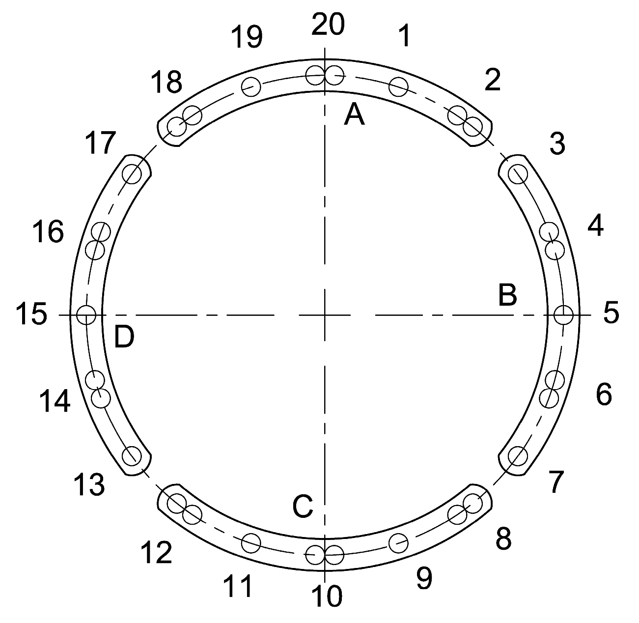
To simplify the control and decrease expenses, thrust cylinders scattered around the perimeter are typically separated into multiple zones. Typical zoning configurations include four-zone, five-zone, six-zone, and so on. Every zone can be considered as a cylinder system that is controlled by valves, and each zone is regulated independently [24]. The attitude of TBM is regulated by manipulating the speed and pressure of each section in order to accomplish tasks such as rectifying misalignment and guiding the machine. Figure 1 displays a typical four-zone structure.

Figure 1.
Distribution diagram of the thrust hydraulic cylinders.
Figure 2 depicts the single-zone principle of the thrust system, which is governed by a PFCV and a PPRV. When the thrust system is operational, the pump’s output flow is directed by PFCV and the directional control valve to the rodless chamber of the hydraulic cylinder, generating the necessary thrust force. TBM’s maximum thrust speed can be regulated by adjusting the flow of PFCV. The magnitude of the thrust force can be modified by modifying the predetermined pressure of PPRV [25]. When PFCV produces an overly high output flow, the surplus oil is directed back to the tank by PPRV. This process ensures that the system’s pressure remains stable. If the system’s pressure is set excessively high, PFCV directs the output flow into the thrust hydraulic cylinder, causing pressure to be solely dictated by the load.
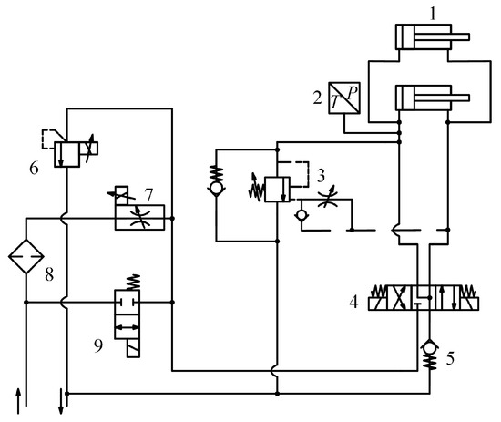
Figure 2.
Grouped working principles diagram of thrust hydraulic system. 1. Thrust hydraulic cylinder; 2. pressure sensor; 3. counterbalance valve; 4. three/four-way directional valve. 5. check valve; 6. PPRV; 7. PFCV; 8. filter; 9. two-way valve.
2.2. Thrust System Modeling
To optimize the simulation process, we omit certain components that have a minor impact on the performance of the investigated thrust system. These components consist of check valves and directional valves in each oil circuit. The thrust system can be simplified to a valve-controlled cylinder system with a PFCV and a PPRV. These valves regulate the thrust speed and pressure, respectively.
The PFCV consists of a constant differential pressure relief valve and a proportional throttle valve connected in a series arrangement. The constant differential pressure relief valve is designed to counteract pressure fluctuations at both ends of the proportional throttle valve [26]. This configuration ensures a consistent difference in pressure at the opening of the throttle valve, enabling the input signal to regulate the flow. The flow via PFCV is solely affected by alterations in the opening of the throttle valve, rather than variations in pressure. In engineering applications, PFCV is often regarded as a typical second-order system. The transfer function expression is as follows [27]:
where represents the flow gain coefficient of PFCV, represents the oscillation frequency of PFCV, and represents the damping ratio of PFCV.
The flow continuity equation for the rodless chamber of the hydraulic cylinder is as follows:
where represents the area of the rodless chamber of the hydraulic cylinder, represents the shield tunneling speed, represents the leakage coefficient of the hydraulic cylinder, represents the pressure in the rodless chamber, represents the volume of the rodless chamber, represents the effective bulk modulus of the hydraulic oil, and is the flow of thrust hydraulic cylinder, which can be obtained from the following equation:
where is output flow of PFCV, is output flow of PPRV.
The force balance equation of the hydraulic cylinder is as follows:
where is the mass of the hydraulic cylinder, and represents the total unknown load, which can be obtained from the following equation:
where is the friction force of the hydraulic cylinder, is the external load force, and is the external disturbance.
The thrust system employs a direct-acting PPRV [28], which regulates the thrust of the spool spring via a proportional solenoid. If the system’s pressure falls below the spring force, the spool will close and direct all oil into the actuator. When the system’s pressure exceeds the solenoid thrust, the spool moves and opens PPRV flow path, causing a portion of the oil to overflow. In engineering applications, PPRV is often regarded as a typical second-order system. The transfer function expression is as follows:
where represents the flow gain coefficient of PPRV, represents the oscillation frequency of PPRV, and represents the damping ratio of PPRV.
3. Design of the Controller
3.1. Design of the Speed Controller
Based on the mathematical models of PFCV and hydraulic cylinder, the state-space equation is established as follows:
where , , are the unknown parameters and is unknown disturbance.
Step 1: The expression for the system’s speed error and its derivative is as follows:
The definition of the Lyapunov function of the system is as follows:
Taking the derivative of it gives the following expression:
To make , the following expression can be obtained as follows:
where .
The solution gives the expression for the virtual control law of , which is .
Since is unknown, its estimated value is denoted by , so can be rewritten as follows:
Redefining the system’s Lyapunov equation is expressed as follows:
where , is the estimation error.
Step 2: The error and its derivative expression are defined as follows:
Differentiating Equation (15) and substituting Equations (14) and (16) yields the following expression:
To make , the adaptive law can be taken as follows:
where .
Redefining the system’s Lyapunov equation is expressed as follows:
Taking the derivative of it and substituting Equation (18) yields the following expression:
To make , the following expression can be obtained:
where .
The solution gives the expression for the virtual control law of , which is :
Step 3: The error and its derivative expression are defined as follows:
Substituting Equations (23) and (24) into gives the following expression:
Redefining the system’s Lyapunov equation is expressed as follows:
Taking the derivative of it gives the following expression:
To make , the following expression can be obtained:
where .
The solution gives the expression for the virtual control law of , which is :
Step 4: The error and its derivative expression are defined as follows:
Substituting Equations (30) and (31) into gives the following expression:
The switching function of the sliding mode system and the exponential approach rate [29] are as follows:
where are the parameters of the controller.
Differentiating Equation (34) and combining it with Equation (35), the control input for PFCV can be obtained as follows:
In Equation (36), represents the equivalent control law, and represents the reaching control law.
The treatment of the unknown parameters gives the following equation as follows:
Since the parameters are unknown, using to denote their estimated values and to denote their estimation errors, respectively, the actual control input expression can be obtained as follows:
Step 5: Redefining the system’s Lyapunov equation is expressed as follows:
where are design parameters.
Taking the derivative of it gives the following expression:
Substituting Equation (38) into gives the following expression:
To make , the adaptive rate of the unknown parameter is chosen as follows:
Step 6: Bringing the adaptive rate of each parameter and the actual input into Equation (41), the following equation can be obtained:
where , .
If is a positive definite matrix, the following expression can be obtained:
Since , and the following expression exists:
By choosing appropriate values, can be guaranteed, which in turn ensures that is a positive definite matrix, thus proving that the system is asymptotically stable.
3.2. Design of the Pressure Controller
Based on the mathematical models of PPRV, the state-space equation is established as follows:
where , are the unknown parameters and is unknown disturbance.
Step 1: The expression for the system’s pressure error and its derivative is as follows:
The switching function of the sliding mode system and the exponential approach rate are as follows:
where are the parameters of the controller.
Differentiating Equation (49) and combining it with Equation (50), the control input for PPRV can be obtained as follows:
In Equation (51), represents the equivalent control law, and represents the reaching control law.
The treatment of the unknown parameters gives the following equation as follows:
Since the parameters are unknown, using to denote their estimated values and to denote their estimation errors, respectively, the actual control input expression can be obtained as follows:
Step 2: Defining the system’s Lyapunov equation is expressed as follows:
where are design parameters.
Taking the derivative of it gives the following expression:
To make , the adaptive rate of the unknown parameter is chosen as follows:
Step 3: Bringing the adaptive rate of each parameter and the actual input into Equation (55), the following equation can be obtained:
Thus, the controller is asymptotically stable and the pressure tracking error tends to zero when system is stabilized.
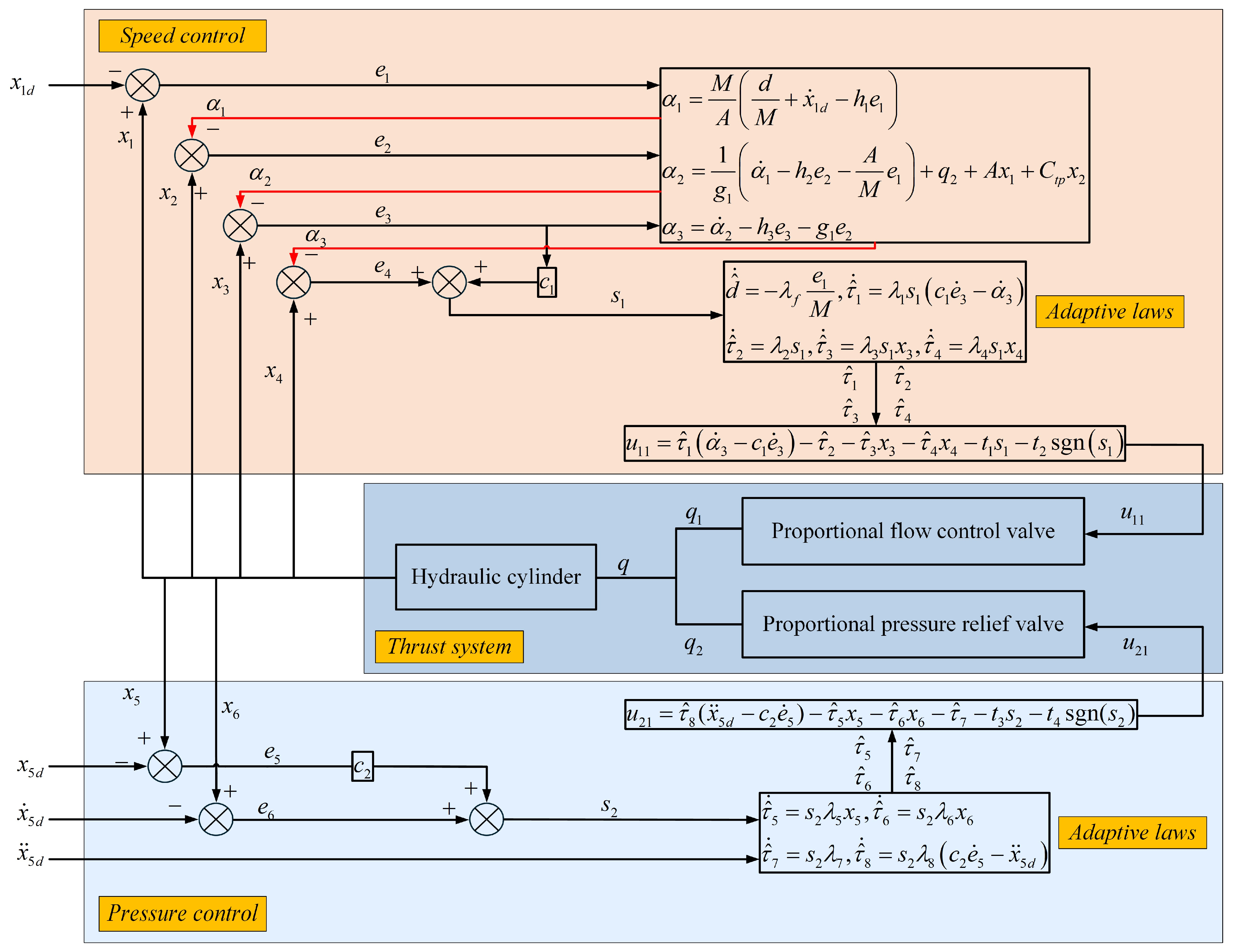
The control module is developed in MATLAB, integrating the speed controller and pressure controller, resulting in the thrust system control block diagram shown in Figure 3.

Figure 3.
Control block diagram of thrust system.
4. Simulation Analysis
The deformation and mechanical relationships caused by TBM in the soil are complex [30]. The main components contributing to the axial resistance of TBM during tunneling are the resistance caused by the cutter head, the friction generated by the shield shell, the friction caused by the sealing brush at the shield tail, and the resistance from the rear support device.
These axial resistances can be classified into two categories: forces that vary with thrust speed, such as the frontal resistance of the cutter head, and forces that remain constant, such as the friction of the shield shell. Therefore, the dynamic relationship between the TBM’s axial resistance and thrust speed can be described using a linear relationship [31]. Consequently, the total axial load on TBM can be expressed as follows:
where is the stratigraphic coefficient, and the corresponding parameter can be selected according to different stratigraphic, and is the load force that does not vary with thrust speed.
PFCV and PPRV are modeled using the HCD library in AMESim. A simplified AMESim model of the thrust system that can be obtained by combining the load model, a PFCV model, and a PPRV model, as shown in Figure 4. To validate the effectiveness of the ASMC algorithm, simulation analysis is conducted in the MATLAB-AMESim environment. The widely used PID control algorithm in practical engineering was chosen for comparison. A comparative analysis of speed and pressure compound control was carried out under conditions such as speed regulation, sudden load changes, and disturbed loads. The main parameters of the joint simulation are shown in Table 1.
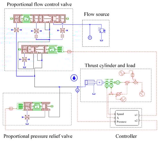
Figure 4.
Simplified AMESim model of the thrust system.

Table 1.
Main parameters of MATLAB-AMESim joint simulation model.
4.1. Simulation and Analysis of Speed Regulation Condition
When the ATA deviates from the DTA during the tunneling process, it is necessary to adjust the thrust speed of each section to minimize the deviation between the axes. During the speed adjustment process, the pressure needs to be controlled to achieve earth pressure balance and reduce the amount of deformation on the surface. The main parameters of the speed regulation process are shown in Table 2 and the simulation results are shown in Figure 5.
Table 2.
Main parameters of speed regulation condition.
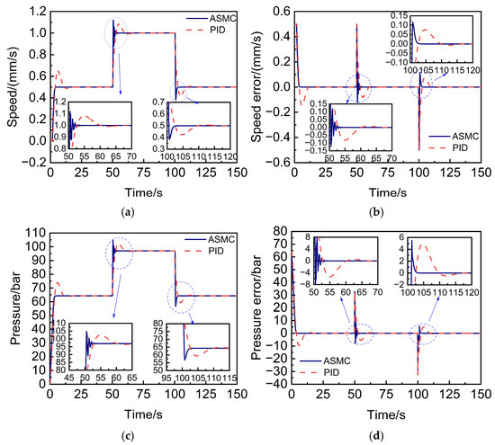
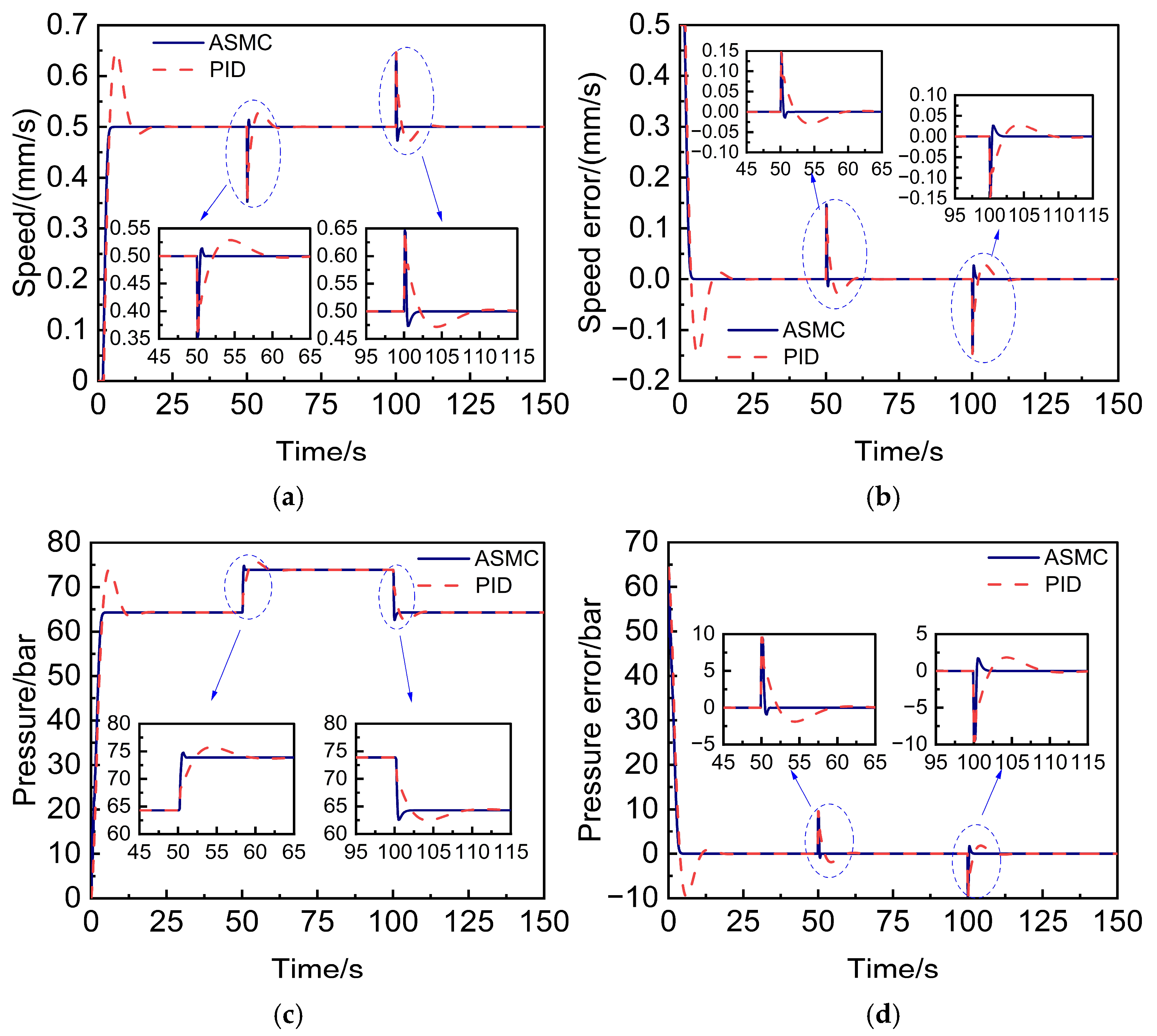
Figure 5.
Simulation results of the speed regulation condition: (a) actual speed; (b) speed tracking error; (c) actual pressure; (d) pressure tracking error.
As shown in Figure 5, when employing the PID control strategy, the initial speed overshoot is approximately 0.13 mm/s, while the pressure overshoot is around 10 bar. The time required for the system’s speed and pressure to reach steady state values is about 15 s. During the speed regulation phase, the speed overshoot is approximately 0.08 mm/s and the pressure overshoot is about 5 bar, with the time to achieve the steady-state values remaining around 15 s. When employing the ASMC, there is virtually no overshoot in speed and pressure during the initial stage, and the time to reach the steady-state values for both speed and pressure is approximately 5 s. In the acceleration phase, there are minor fluctuations in the system’s pressure and speed, with a response time of about 3 s. Notably, there are no fluctuations during the deceleration phase, and the time to reach the steady-state values remains around 3 s. The simulation results demonstrate that the ASMC effectively controls the system to track the desired speed and pressure values during the regulation phase. Compared to the PID controller, the ASMC exhibits nearly no overshoot in the initial phase of speed and pressure, with a response time reduced by approximately 70%. During the speed regulation phase, while the overshoot in speed and pressure remains comparable to that of the PID controller, the response time is shortened by about 80%.
4.2. Simulation and Analysis of a Sudden Changed Load Condition
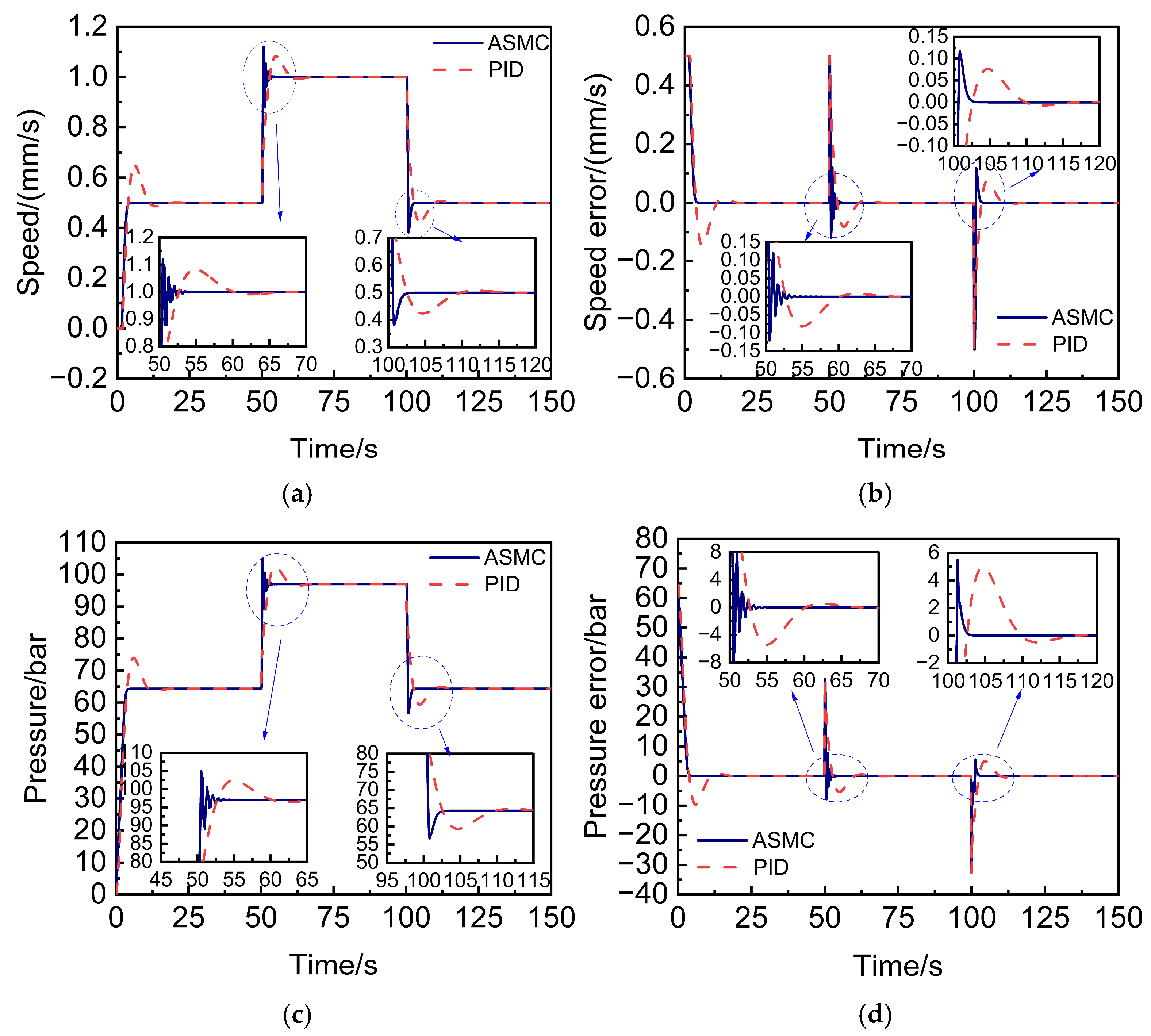
As TBM passes through different strata, the load it experiences changes greatly. At this time, the pressure needs to be adjusted to maintain the earth pressure balance. In this process, the thrust speed needs to be maintained to avoid the ATA deviating from the DTA. The main parameters of the sudden changed load process are shown in Table 3 and the simulation results are shown in Figure 6.
Table 3.
Main parameters of a sudden changed load condition.
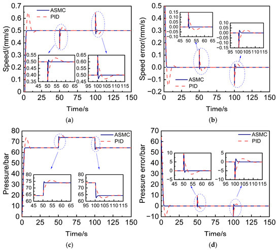
Figure 6.
Simulation results of the sudden changed load condition: (a) actual speed; (b) speed tracking error; (c) actual pressure; (d) pressure tracking error.
As shown in Figure 6, it is evident that under the PID control strategy, when the load is suddenly increased, the response time for the system’s speed and pressure to reach the desired values is approximately 12 s, with a speed overshoot of about 0.04 mm/s and a pressure overshoot of about 2.5 bar. Conversely, when the load is suddenly decreased, the response time is about 10 s, with a speed overshoot of approximately 0.03 mm/s and a pressure overshoot of 2.5 bar. In contrast, under the ASMC, when the load suddenly increases, the system’s response time is about 1.5 s, with a speed overshoot of around 0.01 mm/s and a pressure overshoot of about 1 bar. When the load suddenly decreases, the response time is approximately 2 s. Compared to the PID controller, the ASMC exhibits almost no overshoot in speed and pressure during the initial phase, with the response time being reduced by about 70%. During the process of sudden load changes, the maximum overshoot for both speed and pressure is lower than that of the PID controller, decreasing by approximately 5%, while the response time is reduced by about 80%, allowing the system to achieve a stable state more rapidly.
4.3. Simulation and Analysis of the Disturbed Load Condition
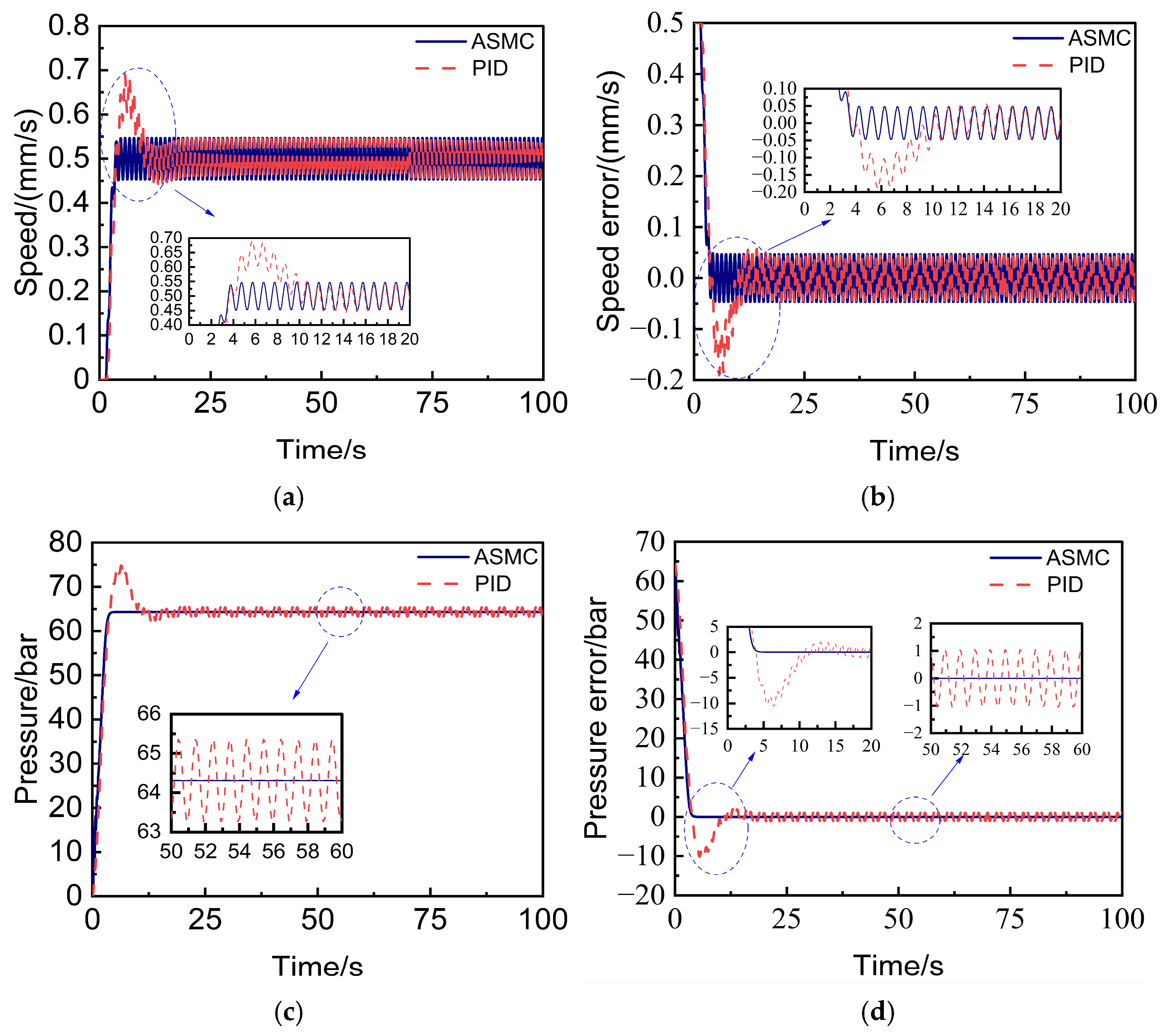
During the actual tunneling process, the ground stratum is often uneven and continuously changing, and the load is in a fluctuating state. Therefore, it is necessary to control the thrust speed and pressure to a stable value to reduce the amount of deformation on the ground surface and ensure the accuracy of trajectory tracking. The main parameters of the disturbed load condition are shown in Table 4 and the simulation results are shown in Figure 7.
Table 4.
Main parameters of disturbed load condition.
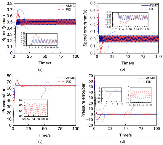
Figure 7.
Simulation results of the disturbed load condition: (a) Actual speed. (b) Speed tracking error. (c) Actual pressure. (d) Pressure tracking error.
As shown in Figure 7, it is evident that under load disturbance conditions, both speed and pressure fluctuate with load changes when using the PID controller. Although the error range of the thrust speed under the ASMC controller is similar to that of the PID controller, the ASMC controller demonstrates a faster response in the initial stage, with pressure remaining almost stable. This capability allows the ASMC controller to effectively maintain the thrust system’s pressure at the desired value. Compared to the PID controller, the ASMC controller exhibits superior adaptability and control performance in the disturbed load condition.
5. Conclusions
In order to ensure the safety of the construction and the accuracy of the trajectory tracking in complex and changing geological conditions, a novel ASMC is proposed to meet the speed–pressure compound control requirements of the thrust system. First, it introduces the principles of a thrust system composed of a PPRV and a PFCV, and establishes its mathematical model. Next, PPRV and PFCV are modeled as a second-order system with unknown dynamic characteristics. By combining this with an ASMC strategy, the pressure and speed control are realized based on system parameter identification. Finally, to validate the performance of the ASMC, a model of the thrust system was built in AMESim. Using the MATLAB-AMESim co-simulation platform, comparative simulation analysis of the compound control of speed and pressure is conducted under speed regulation, sudden changed load, and disturbed load conditions. The simulation results show that the proposed ASMC controller realizes the effect of speed and pressure compound control. Compared with the PID controller, the ASMC controller has almost no overshoot in speed and pressure and the response time is shortened by about 70% in the initial stage. In the speed regulation process and the sudden changed load process, the response time is shortened by about 80%. In the disturbed load process, the ASMC controller can maintain the pressure stability of the thrust system. In conclusion, the ASMC controller significantly improves the response speed and stability of the thrust system, exhibiting better control performance under various operating conditions.
The ASMC algorithm proposed in this paper has shown promising performance in simulation experiments, providing a valuable reference for future research on control theory for TBMs. However, its performance in real-world engineering applications remains uncertain. Therefore, the next step is to further validate the algorithm’s effectiveness and superiority through practical experiments.
Author Contributions
Conceptualization, G.G. and H.Y.; methodology, H.L. and T.X.; formal analysis, L.J. (Lianhui Jia) and L.J. (Lijie Jiang); resources, D.H.; software, H.L. and T.X.; funding acquisition, T.X.; writing—original draft, H.L. and Z.Z.; writing—review and editing, H.L. and Z.Z.; project administration, G.G. and H.Y. All authors have read and agreed to the published version of the manuscript.
Funding
This work received support from the National Key R&D Program of China (Grant No. 2022YFC3802302) and the National Natural Science Foundation of China (No. 52475075).
Data Availability Statement
The data presented in this study are available on request from the corresponding author, within reasonable limits.
Acknowledgments
The authors would like to thank the anonymous reviewers for their valuable suggestions.
Conflicts of Interest
Authors Lianhui Jia and Lijie Jiang were employed by the company China Railway Engineering Equipment Group Co., Ltd. The remaining authors declare that the research was conducted in the absence of any commercial or financial relationships that could be construed as a potential conflict of interest.
References
- Yi, L.G.; Chen, K.; Lu, G.M. Progress in shield tunneling technology for urban underground space in China. Tunn. Constr. 2024, 44, 1. [Google Scholar]
- Bai, Y.; Gao, P.; Ren, R. Research on simulation control of shield machine propulsion hydraulic system. Mod. Manuf. Eng. 2020, 480, 128. [Google Scholar]
- Li, J.K.; Yan, B. The monitoring and analysis of surface subsidence of soft soil rock large section of subway tunnel shield construction. Adv. Mater. Res. 2014, 848, 78–82. [Google Scholar] [CrossRef]
- Meng, F.; Chen, P.; Kang, X. Effects of tunneling induced soil disturbance on the post- construction settlement in structured soft soil. Tunn. Undergr. Space Technol. 2018, 80, 53–63. [Google Scholar] [CrossRef]
- Pourtaghi, A.; Lotfollahi-Yaghin, M. Wavenet ability assessment in comparison to ANN for predicting the maximum surface settlement caused by tunneling. Tunn. Undergr. Space Technol. 2012, 28, 257–271. [Google Scholar] [CrossRef]
- Zhang, L.; Wu, X.; Ji, W.; Simaan, M. Intelligent approach to estimation of tunnel-induced ground settlement using wavelet packet and support vector machines. J. Comput. Civ. Eng. 2017, 31, 04016053. [Google Scholar] [CrossRef]
- Bouayad, D.; Emeriault, F. Modeling the relationship between ground surface settlements induced by shield tunneling and the operational and geological parameters based on the hybrid PCA/ANFIS method. Tunn. Undergr. Space Technol. 2017, 68, 142–152. [Google Scholar] [CrossRef]
- Moeinossadat, S.; Ahangari, K. Estimating maximum surface settlement due to EPBM tunneling by Numerical Intelligent approach: A case study Tehran subway line 7, Tehran, Iran. Transp. Geotech. 2018, 18, 92–102. [Google Scholar] [CrossRef]
- Moghaddasi, R.; Noorian, M. ICA-ANN, ANN and multiple regression models for prediction of surface settlement caused by tunneling. Tunn. Undergr. Space Technol. 2018, 79, 197–209. [Google Scholar] [CrossRef]
- Koopialipoor, M.; Fahimifar, A.; Ghaleini, E. Development of a new hybrid ANN for solving a geotechnical problem related to tunnel boring machine performance. Eng. Comput. 2020, 36, 345–357. [Google Scholar] [CrossRef]
- Libin, T.; SeonHong, N. Comparison of machine learning methods for ground settlement prediction with different tunneling datasets. J. Rock Mech. Geotech. Eng. 2021, 13, 1274–1289. [Google Scholar]
- Hussaine, S.; Linlong, M. Intelligent prediction of maximum ground settlement induced by EPB shield tunneling using automated machine learning techniques. Mathematics 2022, 10, 4637. [Google Scholar] [CrossRef]
- Yazdanparast, M.; Koushkgozar, H.; Hassanpour, J. Predicting maximum settlement induced by EPB shield tunneling through image processing and an intelligent approach. KSCE J. Civ. Eng. 2024, 28, 4076–4087. [Google Scholar] [CrossRef]
- Ren, Y.; Sun, Z.; Chu, C. An Attitude Control Strategy for Shield Thrusting. Tunn. Constr. 2019, 39, 1038–1044. [Google Scholar]
- Li, S.; Cao, X. Synchronous Control Characteristics Analysis of Shield Propulsion Hydraulic System Based on Tracking Differentiator and Self-Adaptive Nonlinear PID. Int. J. Pattern Recognit. Artif. Intell. 2021, 35, 2159053. [Google Scholar] [CrossRef]
- Li, G.; Niu, Y.; Chen, K. Research on hydraulic thrusting control system of shield machine based on BP-PID controller. Tunn. Constr. 2017, 37, 885. [Google Scholar]
- Liu, X.; Ma, L. Study on deviation correction control of shield machine based on PSO-PID. Comput. Meas. Control 2020, 28, 122–126. [Google Scholar]
- Gambhire, S.J.; Kishore, D.R.; Londhe, P.S. Review of sliding mode based control techniques for control system applications. Int. J. Dyn. Control 2021, 9, 363–378. [Google Scholar] [CrossRef]
- Bakhshande, F.; Bach, R.; Söffker, D. Robust control of a hydraulic cylinder using an observer-based sliding mode control: Theoretical development and experimental validation. Control Eng. Pract. 2020, 95, 104272. [Google Scholar] [CrossRef]
- Zhao, Y.; Qiu, C.; Huang, J. Terminal Sliding Mode Force Control Based on Modified Fast Double-Power Reaching Law for Aerospace Electro-Hydraulic Load Simulator of Large Loads. Actuators 2024, 13, 145. [Google Scholar] [CrossRef]
- Lao, L.; Chen, P. Adaptive Sliding Mode Control of an Electro-Hydraulic Actuator with a Kalman Extended State Observer. IEEE Access 2024, 12, 8970–8982. [Google Scholar] [CrossRef]
- Lu, S.; E, D.C.; Dong, X. Hydraulic cylinder displacement tracking control based on improved adaptive high-order sliding mode. Mach. Tool Hydraul. 2023, 51, 144–149. [Google Scholar]
- Zhang, J.; Wang, C.; Zhao, E. Compound sliding mode control of double-pump sub-chamber electro-hydraulic load-simulation system. Mach. Tool Hydraul. 2024, 52, 124–132. [Google Scholar]
- Shi, H.; Gong, G.; Yang, H. Electro-hydraulic proportional control of thrust system for shield tunneling machine. Autom. Constr. 2009, 18, 950–956. [Google Scholar]
- Gong, G.; Hu, G.; Yang, H. Control analysis of thrust hydraulic system for shield tunnelling machine. Zhongguo Jixie Gongcheng/China Mech. Eng. 2007, 18, 1391–1395. [Google Scholar]
- Zhang, W.; Yuan, Q.; Xu, Y. Research on control strategy of electro-hydraulic lifting system based on AMESim and MATLAB. Symmetry 2023, 15, 435. [Google Scholar] [CrossRef]
- Li, Y.; Wang, Q. Adaptive robust tracking control of a proportional pressure-reducing valve with dead zone and hysteresis. Trans. Inst. Meas. Control 2018, 40, 2151–2166. [Google Scholar] [CrossRef]
- Chen, J.; Li, J.; Liu, Y. Simulated loading experiment of proportional relief valve in the hydraulic system. Mach. Tool Hydraul. 2020, 48, 58–61. [Google Scholar]
- Guo, X.; Wang, C.; Liu, H. Extended-state-observer based sliding mode control for pump-controlled electro-hydraulic servo system. J. Beijing Univ. Aeronaut. Astronaut. 2020, 46, 1159–1168. [Google Scholar]
- Wang, X.; Yuan, D.; Jin, D. Determination of thrusts for different cylinder groups during shield tunneling. Tunn. Undergr. Space Technol. 2022, 127, 104579. [Google Scholar] [CrossRef]
- Sugimoto, M.; Sramoon, A. Theoretical model of shield behavior during excavation. I: Theory. J. Geotech. Geoenvironmental Eng. 2002, 128, 138–155. [Google Scholar] [CrossRef]


Disclaimer/Publisher’s Note: The statements, opinions and data contained in all publications are solely those of the individual author(s) and contributor(s) and not of MDPI and/or the editor(s). MDPI and/or the editor(s) disclaim responsibility for any injury to people or property resulting from any ideas, methods, instructions or products referred to in the content. |
© 2025 by the authors. Licensee MDPI, Basel, Switzerland. This article is an open access article distributed under the terms and conditions of the Creative Commons Attribution (CC BY) license (https://creativecommons.org/licenses/by/4.0/).