Event-Driven Prescribed-Time Tracking Control for Multiple UAVs with Flight State Constraints

Abstract

Consensus tracking control for multiple UAVs demonstrates critical theoretical value and application potential, improving system robustness and addressing challenges in complex operational environments. This paper addresses the challenge of event-triggered prescribed-time synchronization tracking control for 6-DOF fixed-wing UAVs with state constraints. We propose a novel prescribed-time command filtered backstepping approach to effectively tackle the issues of complexity explosion and singularities. By utilizing a state-transition function, we manage asymmetric time-varying state constraints, including limitations on speed, roll, yaw, and pitch angles in UAVs. The theoretical analysis demonstrates that all signals in the 6-DOF UAV system remain bounded, with tracking errors converging to the origin within the prescribed time. Finally, simulation results validate the effectiveness of the proposed control strategy.

1. Introduction

With the widespread adoption of unmanned aerial vehicles (UAVs) in both military and civilian sectors, the cooperative control of multiple UAVs has garnered significant attention [1,2,3,4]. UAVs are characterized by their intelligence, lightweight design, and cost effectiveness [5]. Over the past few decades, distributed optimization has been extensively employed in multi-agent systems [6,7]. Researchers design optimal trajectories for multi-agent systems based on distributed optimization methods [8], and demonstrated effectiveness in addressing nonlinear dynamics and non-convex constraints [9].

However, recent practical applications require faster convergence rates and enhanced robustness. To address these demands, finite-time control designs have been proposed [10,11,12,13,14], enabling systems to achieve rapid convergence within a finite time. However, the settling time for finite-time stability is dependent on the system’s initial state, meaning convergence may take longer if the initial state is large. To resolve this, fixed-time control methods have been developed [15,16,17,18], ensuring that the convergence time is independent of the initial state. Despite this improvement, the settling time in fixed-time stabilization remains a complex function influenced by system parameters and cannot be predefined. In many UAV applications, it is critical to prescribe the convergence time in advance. Thus, prescribed-time and predefined-time stability methods were introduced, allowing the settling time to be determined by specific parameters [19,20]. Several predefined-time sliding-mode controllers have been developed to ensure fast response and robust steady-state performance [21,22,23]. To further enhance dynamic performance in the presence of actuator saturation and system uncertainties, a vision-based prescribed performance controller was introduced [24], along with a modified predefined-time control scheme for specialized missions, such as UAV in-air refueling [25]. However, most studies model UAVs with only three degrees of freedom, which does not accurately capture UAV motion compared to the more comprehensive six-degrees-of-freedom model. This makes the design of prescribed-time controllers for 6-DOF UAVs significantly more challenging.

In practical flight, external disturbances [26] and model uncertainties [27] pose challenges to the stability of UAVs. By employing disturbance observers to estimate and counteract these effects while dynamically adjusting controller parameters via online learning mechanisms such as neural networks, adaptive control ensures robust performance compensation for both environmental perturbations and system modeling errors [28,29]. Meanwhile, the effects of aerodynamics and the flight environment must be taken into account, making it essential to impose state constraints on the speed and attitude control of UAVs to ensure safe system operation. Several approaches have been proposed to address this challenge, including reference governors [30], extremum-seeking methods [31], and barrier Lyapunov functions (BLF) [32]. Additionally, a higher-order tan-type BLF was introduced in [33] for UAV systems, resulting in improved tracking performance, while a time-varying BLF was employed in [34] to handle state constraints. In [18], an IBLF-based controller was developed to impose both upper and lower positive constraints on non-negative states. Moreover, a nonlinear function was proposed in [35] to transform constrained systems into unconstrained ones. Despite these advances, few studies have simultaneously addressed state constraints in both the speed and attitude subsystems, particularly in 6-DOF UAV systems.

In recent years, event-triggered control (ETC) has been developed to conserve communication and computational resources [36,37]. For instance, an event-triggered super-twisting algorithm for UAVs facing external disturbances was proposed in [38], effectively reducing computational costs while maintaining system performance. Similarly, Ref. [39] designed an adaptive event-triggered mechanism for quadrotor UAVs, achieving practical finite-time stability. In [40], a novel event-based dynamic sliding-mode surface was introduced to ensure robust stabilization of multi-quadrotor systems under unknown perturbations. However, most existing ETC methods primarily focus on attitude systems and finite-time stability [40,41,42]. Thus, further research is needed to develop a novel prescribed-time-based event-triggered control scheme for UAV systems.

Motivated by the discussions above, the main contributions of this paper are outlined as follows:

• Unlike existing works [24,25,43], this paper designs an event-triggered prescribed-time backstepping control for 6-DOF UAV systems. The stability proof of the closed-loop system under the proposed method is proved by Lyapunov-based technology.
• By proposing a novel prescribed-time command-filtered backstepping, the “explosion of complexity” problem is effectively addressing while ensuring prescribed-time stability and a fast response.
• In contrast to the works [18,33,34,35] that utilize barrier Lyapunov functions to tackle state-constrained problems, this paper addresses the issue of asymmetric time-varying state constraints by employing a state-transition function. This approach effectively eliminates the need for feasibility conditions on the virtual controller.

The rest of this paper is organized as follows:

In Section 2, we present the preliminaries and problem formulation. The prescribed-time event-triggered control design and stability analysis are developed in Section 3. Section 4 provides the simulation results, while Section 5 concludes the paper.

2. Preliminaries and Problem Formulation

2.1. Notations

${\mathfrak{R}}^{n\times n}$ denotes real $m\times n$ matrices, $|·|$ denotes the absolute value, and $\parallel ·\parallel$ represents the Euclidean 2-norm of a vector or matrix. ${\lambda }_{min}\left(A\right)$ is the minimum eigenvalues of the matrix A, $S(·)$ is skew-symmetric matrix, and $(·)$ is the signum function; for $\mathit{b}={[b_1,b_2,b_3]}^{\mathrm{T}}$, define ${\mathrm{sig}}^a\left(\mathit{b}\right)=[\mathrm{sign}\left(b_1\right)|b_1{|}^a,\mathrm{sign}\left(b_2\right){\left|b_2\right|}^a,$ $\mathrm{sign}\left(b_3\right)|b_3{{|}^a]}^{\mathrm{T}}$, where a is a constant.

2.2. UAV Dynamics Model

A fixed-wing UAV system is assumed to have N UAVs. The connections among UAVs are described as an undirected graph $\mathcal{G}=(\mathcal{V},\mathcal{E},\mathcal{A})$ with $\mathcal{V}=\{v_1,\dots v_n\}$ being the set of nodes, and $\mathcal{E}=\left\{\right(i,j),i,j\in \mathcal{V},$ and $i\ne j\}$ being the edges. $\mathcal{A}=\left[a_{ij}\right]\in {\mathfrak{R}}^{n\times n}$ denotes the weighted adjacency matrix of $\mathcal{G}$, where $a_{ij}>0$ if the node j is node i’s neighbor, and zero otherwise. Meanwhile, we suppose $a_{ii}=0$. The Laplacian matrix is defined by $\mathcal{L}=\mathcal{D}-\mathcal{A}$, where $\mathcal{D}=\mathrm{diag}\{d_1,\dots d_n\}$ with $d_i={\sum }_{j=1}^n{a}_{ij}$. When there exists a path from every node to every other node, $\mathcal{G}$ is connected.

Consider a group of N fixed-wing UAVs. The dynamics model of ith UAV is described as [43,44].

$$\begin{array}{c}\hfill \left\{\begin{array}{c}{\dot{\mathit{p}}}_i={\mathit{R}}_1\left({\mathit{\phi }}_i\right){\mathit{v}}_i\hfill \\ {\dot{\mathit{v}}}_i=-\mathit{S}\left({\mathit{\omega }}_i\right){\mathit{v}}_i+{\mathit{R}}_1^{\mathrm{T}}\left({\mathit{\phi }}_i\right)\mathit{g}+{\displaystyle \frac{{\mathit{T}}_i+{\mathit{F}}_i}{m_i}}+{\mathit{d}}_{vi}\hfill \\ {\dot{\mathit{\phi }}}_i={\mathit{R}}_2^{-1}\left({\mathit{\phi }}_i\right){\omega }_i\hfill \\ {\mathit{J}}_i{\dot{\mathit{\omega }}}_i=-{\mathit{\omega }}_i\times {\mathit{J}}_i{\mathit{\omega }}_i+{\mathit{N}}_i+{\mathit{C}}_i{\delta }_i+{\mathit{J}}_i{\mathit{d}}_{\mathit{\omega }i},\hfill \end{array}\right.\end{array}$$

(1)

where ${\mathit{p}}_i={[x_i,y_i,z_i]}^{\mathrm{T}}$ and ${\mathit{\phi }}_i={[{\varphi }_i,{\theta }_i,{\psi }_i]}^{\mathrm{T}}$ represent the inertial position and attitude angle, ${\mathit{v}}_i={[{\alpha }_i,{\varrho }_i,o_i]}^{\mathrm{T}}$ and ${\mathit{\omega }}_i={[l_i,q_i,j_i]}^{\mathrm{T}}$ denote the linear speed and angular velocity, ${\mathit{T}}_i={[T_{Xi},0,0]}^{\mathrm{T}}$ represents thrust vector, and ${\delta }_i={[{\delta }_{ei},{\delta }_{ai},{\delta }_{ri}]}^{\mathrm{T}}$ represents control surfaces; $\mathit{g}={[0,0,g]}^{\mathrm{T}}$ is the gravity acceleration. ${\mathit{d}}_{vi}$ and ${\mathit{d}}_{\omega i}$ are external disturbances. ${\mathit{R}}_1\left({\mathit{\phi }}_i\right)$ is the rotation matrix transforming the body frame coordinates to inertial axis coordinates, and ${\mathit{R}}_2\left({\mathit{\phi }}_i\right)$ is the time derivative of attitude angles.

$$\begin{array}{cc}\hfill {\mathit{R}}_{\mathit{1}}\left({\mathit{\phi }}_{\mathit{i}}\right)& =\left[\begin{array}{ccc}{c}_{\psi i}{c}_{\theta i}& -s_{\psi i}{s}_{\varphi i}+c_{\psi i}{s}_{\theta i}{s}_{\varphi i}& s_{\psi i}{s}_{\varphi i}+c_{\psi i}{s}_{\theta i}{c}_{\varphi i}\\ s_{\psi i}{c}_{\theta i}& c_{\psi i}{c}_{\varphi i}+s_{\psi i}{s}_{\theta i}{s}_{\varphi i}& -c_{\psi i}{s}_{\varphi i}+s_{\psi i}{s}_{\theta i}{c}_{\varphi i}\\ -s_{\theta i}& c_{\theta i}{s}_{\varphi i}& c_{\theta i}{c}_{\varphi i}\end{array}\right]\hfill \end{array}$$

(2)

$$\begin{array}{cc}\hfill {\mathit{R}}_{\mathit{2}}\left({\mathit{\phi }}_{\mathit{i}}\right)& =\left[\begin{array}{ccc}1& 0& -s_{\psi i}\\ 0& c_{\psi i}& s_{\psi i}{c}_{\theta i}\\ 0& -s_{\theta i}& c_{\psi i}{c}_{\theta i}\end{array}\right],\hfill \end{array}$$

(3)

where c and s are the abbreviation of sin and cos, respectively. J is the inertia tensor and $C_i$ is the control matrix, which are given as

$$\begin{array}{cc}\hfill J& =\left[\begin{array}{ccc}{J}_{xi}& 0& -J_{xzi}\\ 0& J_{yi}& 0\\ -J_{zxi}& 0& J_{zi}\end{array}\right]\hfill \end{array}$$

(4)

$$\begin{array}{cc}\hfill C_i& ={\displaystyle \frac{1}{2}}\rho V_i^2{S}_i\left[\begin{array}{ccc}{b}_i{c}_{l\delta ai}& 0& b_i{c}_{l\delta ri}\\ 0& {\overline{c}}_i{c}_{m\delta ei}& 0\\ b_i{c}_{n\delta ai}& 0& b_i{c}_{n\delta ri}\end{array}\right],\hfill \end{array}$$

(5)

where $\rho$ is the air density, $S_i$ is the wing surface area, $b_i$ is the wingspan, ${\overline{c}}_i$ is the mean aerodynamic chord, and $c_{l\delta ai}$, $c_{l\delta ri}$, $c_{m\delta ei}$, $c_{n\delta ai}$ and $c_{n\delta ri}$ are the coefficients.

The aerodynamic force vector $F_i$ is calculated as

$$F_i={\displaystyle \frac{1}{2}}\rho V_i^2{S}_i{R}_3^{-1}\left({\alpha }_i,{\beta }_i\right)\left[\begin{array}{c}-C_{Di}\\ C_{Yi}\\ -C_{Li}\end{array}\right],$$

(6)

where ${\alpha }_i=arctan(o_1/{\alpha }_i)$ and ${\beta }_i=arctan({\alpha }_i/{\varrho }_i)$, $C_{Di}$, $C_{Yi}$, and $C_{Li}$ are the coefficients. The matrix $R_3\left({\alpha }_i,{\beta }_i\right)$ is

$$R_3\left({\alpha }_i,{\beta }_i\right)=\left[\begin{array}{ccc}{c}_{\alpha i}{c}_{\beta i}& s_{\beta i}& s_{\alpha i}{c}_{\beta i}\\ -c_{\alpha i}{s}_{\beta i}& c_{\beta i}& -s_{\alpha i}{s}_{\beta i}\\ -s_{\alpha i}& 0& c_{\alpha i}\end{array}\right].$$

(7)

Additionally, the aerodynamic moment vector $N_i$ is calculated as

$$N_i={\displaystyle \frac{1}{2}}\rho V_i^2{S}_i\left[\begin{array}{c}{b}_i{C}_{li}^{\prime }\\ {\overline{c}}_i{C}_{Mi}^{\prime }\\ b_i{C}_{ni}^{\prime }\end{array}\right],$$

(8)

where $C_{li}^{\prime }$, $C_{Mi}^{\prime }$ and $C_{ni}^{\prime }$ are coefficients, of which the details are introduced in [43].

2.2.1. Velocity Subsystem

Based on (1), the velocity can be differentiated as

$${\dot{V}}_i={\displaystyle \frac{{\alpha }_i{T}_{xi}}{m_i{V}_i}}+{\displaystyle \frac{{\mathit{v}}_i^{\mathrm{T}}}{V_i}}({\mathit{R}}_1^{\mathrm{T}}\mathit{g}+{\displaystyle \frac{{\mathit{F}}_{i0}}{m_i}})+{\displaystyle \frac{{\mathit{v}}_i^{\mathrm{T}}}{V_i}}({\Delta }_{vi}+{\mathit{d}}_{vi}),$$

(9)

where ${\Delta }_{vi}={\displaystyle \frac{\Delta {\mathit{F}}_i}{m_i}}$ represents the modeling uncertainties in the velocity subsystem.

2.2.2. Attitude Subsystem

$$\begin{array}{c}\hfill \left\{\begin{array}{c}{\dot{\mathit{\phi }}}_i={\mathit{R}}_2^{-1}\left({\mathit{\phi }}_i\right){\mathit{\omega }}_i\hfill \\ {\dot{\mathit{\omega }}}_i={\mathit{J}}_{i0}^{-1}\mathit{S}\left({\mathit{J}}_{i0}{\mathit{\omega }}_i\right)+{\mathit{J}}_{i0}^{-1}{\mathit{N}}_{i0}+{\mathit{J}}_{i0}^{-1}{\mathit{C}}_{i0}{\mathit{\delta }}_i+{\Delta }_{\omega i}+{\mathit{d}}_{\omega i},\hfill \end{array}\right.\end{array}$$

(10)

where ${\Delta }_{\omega i}=\Delta {\mathit{J}}_i^{-1}\mathit{S}\left({\mathit{J}}_i{\mathit{\omega }}_i\right)+\Delta {\mathit{J}}_i^{-1}{\mathit{N}}_i+\Delta {\mathit{J}}_i^{-1}{\mathit{C}}_i{\delta }_i$ represents the lumped uncertainties induced by modeling uncertainties in the attitude subsystem.

Assumption 1.

The speed reference signal is restricted to $V_{li}\left(t\right)<V_{xi}<V_{ui}\left(t\right)$. The attitude reference signal is restricted to ${\mathit{\phi }}_{li}\left(t\right)<{\mathit{\phi }}_i<{\mathit{\phi }}_{ui}\left(t\right)$. $V_{li}\left(t\right)$, $V_{ui}\left(t\right)$, ${\mathit{\phi }}_{li}\left(t\right)$, and ${\mathit{\phi }}_{ui}\left(t\right)$ are time-varying smooth and positive functions.

Assumption 2.

The external disturbance ${\mathit{d}}_{vi}$ and ${\mathit{d}}_{\omega i}$ are bounded.

Assumption 3.

There exists a positive constant $q_0$ such that ${\lambda }_{min}\left(J_{i0}^{-1}{C}_{i0}\right.$ $\left.D_{\phi }{\left(J_{i0}^{-1}{C}_{i0}\right)}^{\mathrm{T}}\right)$ $\ge q_0$.

2.3. State Transition

In order to transform the constrained system into the nonconstrained system, a nonlinear function is introduced that maps the system state from space ${\Omega }_x$ to space ${\Omega }_{\mathrm{\Phi }}$.

$$\mathrm{\Phi }\left(x\left(t\right)\right)={\displaystyle \frac{x\left(t\right)}{(m_1\left(t\right)+x\left(t\right))(m_2\left(t\right)-x\left(t\right))}}.$$

(11)

Taking the derivative of (11), it has

$$\dot{\mathrm{\Phi }}\left(x\left(t\right)\right)=p\dot{x}\left(t\right)+q,$$

(12)

where $x\left(t\right)$ is a constrained system, $\mathrm{\Phi }\left(x\right(t\left)\right)$ is a nonconstrained system, $m_1\left(t\right)$ and $m_2\left(t\right)$ are positive time-varying functions, $p={\displaystyle \frac{m_1{m}_2+x^2}{{(m_1+x)}^2{(m_2-x)}^2}}$, $q={\displaystyle \frac{-[{\dot{m}}_1{m}_2+m_1{\dot{m}}_2+({\dot{m}}_2-{\dot{m}}_1)x]x}{{(m_1+x)}^2{(m_2-x)}^2}}$.

According to (12), if $-m_1\left(t\right)<x\left(t\right)<m_2\left(t\right)$, $\mathrm{\Phi }\left(x\right(t\left)\right)$ is monotonically increasing. For any initial condition $x\left(0\right)$, if $-m_1\left(0\right)<x\left(0\right)<m_2\left(0\right)$, then $-m_1\left(t\right)<x\left(t\right)<m_2\left(t\right)$ always holds. By using (11), the constrained system can be transformed into nonconstrained system.

2.4. Control Objective

This study aims to design an event-triggered tracking controller that ensures the consistent tracking of both velocity and attitude within a prescribed time, all while adhering to specified velocity and attitude constraints.

To design the prescribed-time event-triggered controller, several lemmas are introduced.

Lemma 1

([45]). Consider a nonlinear system

$$\dot{x}\left(t\right)=f\left(x\left(t\right)\right),x_0=x\left(0\right),$$

(13)

suppose that there exists a radially unbounded Lyapunov function $V\left(x\right)$ such that

$$\dot{V}\left(x\right)\le -{\displaystyle \frac{\pi }{\mu T_c\sqrt{{\kappa }_1{\kappa }_2}}}({\kappa }_1{V}^{1-{\displaystyle \frac{\mu }{2}}}\left(x\right)+{\kappa }_2{V}^{1+{\displaystyle \frac{\mu }{2}}}\left(x\right))+\varpi ,$$

(14)

where ${\kappa }_1>0$, ${\kappa }_2>0$, $T_c>0$, $0<\mu <1$, $0<\varpi <+\infty$; then, the nonlinear system is practically predefined-time stable, and the residual set of the solutions of system (13) can be given by

$$V\left(x\right)\le min\left\{{\left({\displaystyle \frac{\varpi \mu T_c\sqrt{{\kappa }_1{\kappa }_2}}{\pi {\kappa }_1(1-\theta )}}\right)}^{{\displaystyle \frac{2}{2-\mu }}},{\left({\displaystyle \frac{\varpi \mu T_c\sqrt{{\kappa }_1{\kappa }_2}}{\pi {\kappa }_2(1-\theta )}}\right)}^{{\displaystyle \frac{2}{2+\mu }}}\right\},$$

(15)

where $\theta \in (0,1)$, the settling time is given by $T_{pc}={\displaystyle \frac{T_c}{\sqrt{\theta }}}$.

Lemma 2

([46]). For $x_i\in \mathbb{R},i\in \mathcal{N}$, then

$${\left(\sum _{i=1}^n\left|x_i\right|\right)}^b\le \sum _{i=1}^n{\left|x_i\right|}^b\le n^{1-b}{\left(\sum _{i=1}^n\left|x_i\right|\right)}^b,$$

(16)

if $b\ge 1$, then

$$\sum _{i=1}^n{\left|x_i\right|}^b\ge n^{1-b}{\left(\sum _{i=1}^n\left|x_i\right|\right)}^b.$$

(17)

Lemma 3

([47]). For $x\in \mathbb{R},y\in \mathbb{R},c_1,c_2,c_3$ are positive constants; then,

$${\left|x\right|}^{c_1}{\left|y\right|}^{c_2}\le {\displaystyle \frac{c_1}{c_1+c_2}}{c}_3{\left|x\right|}^{c_1+c_2}+{\displaystyle \frac{c_2}{c_1+c_2}}{c}_3^{-{\displaystyle \frac{c_1}{c_2}}}{\left|y\right|}^{c_1+c_2}.$$

(18)

Lemma 4

([48]). For $y\in \mathbb{R},\varsigma \in \mathbb{R},$ and $\varsigma >0$, then

$$0\le \left|y\right|-ytanh\left({\displaystyle \frac{y}{\varsigma }}\right)\le 0.2785\varsigma .$$

(19)

Lemma 5

([49]). For $x\in \mathbb{R},\iota \in \mathbb{R},$ and $\iota >0$, then

$$0\le \left|x\right|-{\displaystyle \frac{x^2}{\sqrt{x^2+\iota }}}\le \sqrt{\iota }.$$

(20)

Lemma 6

([50]). For $x,y\in \mathbb{R},y\ge x,$ and positive $b>0$, then

$$y{\left(x-y\right)}^b\le {\displaystyle \frac{b}{1+b}}\left(x^{1+b}-y^{1+b}\right).$$

(21)

Lemma 7

([51]). For the nonlinear function $\Delta \left(\Theta \right):{\Re }^N\to \Re$ within a given compact set $\Omega \left(\Theta \right)\subset {\Re }^N$, there exist the radial-basis-function neural networks such that

$$\Delta \left(\Theta \right)={{\mathit{W}}^{*}}^{\mathrm{T}}\mathrm{h}\left(\Theta \right)+g\left(\Theta \right).$$

(22)

where ${\mathit{W}}^{*}={\left[{\overline{\mathit{W}}}_1,{\overline{\mathit{W}}}_2,\dots ,{\overline{\mathit{W}}}_n\right]}^{\mathrm{T}}$ denotes the idealized weight matrix, $g\left(\Theta \right)$ is the bounded approximation error, and $\mathit{h}\left(\Theta \right)={\left[{\overline{\mathit{h}}}_1\left(\Theta \right),{\overline{\mathit{h}}}_2\left(\Theta \right),\dots ,{\overline{\mathit{h}}}_n\left(\Theta \right)\right]}^{\mathrm{T}}$ is the basis function vector.

3. Prescribed-Time Control Design

3.1. Error Transformations Based on State Transition

3.1.1. Velocity Subsystem

Define the velocity-tracking error

$$e_{vi}={\beta }_{1i}\left(V_i-V_d\right)+{\beta }_{2i}\sum _{j\in N_i}{a}_{ij}\left(V_i-V_j\right),$$

(23)

where ${\beta }_{1i},{\beta }_{2i}$ are positive design parameters.

According to (11), the tracking error $e_{vi}$ is transformed into

$${\mathrm{\Phi }}_{vi}={\displaystyle \frac{e_{vi}}{\left(V_{li}+e_{vi}\right)\left(V_{ui}-e_{vi}\right)}}.$$

(24)

Taking the derivative of (24), it has

$$\begin{array}{cc}\hfill {\dot{\mathrm{\Phi }}}_{vi}& =p_{vi}{\dot{e}}_{vi}+q_{vi}\hfill \end{array}$$

(25)

$$\begin{array}{cc}\hfill p_{vi}& ={\displaystyle \frac{V_{li}{V}_{ui}+e_{vi}^2}{{(V_{li}+e_{vi})}^2{(V_{ui}-e_{vi})}^2}}\hfill \end{array}$$

(26)

$$\begin{array}{cc}\hfill q_{vi}& ={\displaystyle \frac{-\left[{\dot{V}}_{li}{V}_{ui}+V_{li}{\dot{V}}_{ui}+\left({\dot{V}}_{ui}-{\dot{V}}_{li}\right)e_{vi}\right]e_{vi}}{{(V_{li}+e_{vi})}^2{(V_{ui}-e_{vi})}^2}}.\hfill \end{array}$$

(27)

3.1.2. Attitude Subsystem

Define the attitude-tracking error

$${\mathit{e}}_{\phi i}={\beta }_{3i}\left({\mathit{\phi }}_i-{\mathit{\phi }}_d\right)+{\beta }_{4i}\sum _{j\in N_i}{a}_{ij}\left({\mathit{\phi }}_i-{\mathit{\phi }}_j\right),$$

(28)

where ${\beta }_{3i},{\beta }_{4i}$ are positive design parameters.

Similarly, we have

$${\dot{\mathbf{\Phi }}}_{\phi i}={\mathit{p}}_{\phi i}{\dot{\mathit{e}}}_{\phi i}+{\mathit{q}}_{\phi i},$$

(29)

where ${\mathit{p}}_{\phi i}=\mathrm{diag}(p_{\phi i\varphi },p_{\phi i\theta },p_{\phi i\psi })$, ${\mathit{q}}_{\phi i}=[q_{\phi i\varphi },q_{\phi i\theta },$ $q_{\phi i\psi }{]}^{\mathrm{T}}$.

Remark 1.

Noting that $p_{vi},q_{vi},{\mathit{p}}_{\phi i},{\mathit{q}}_{\phi i}$ are time-varying parameters, which are affected by tracking errors and state constraints. When designing the controller, we only need to guarantee the boundedness of ${\mathrm{\Phi }}_{vi}$ and ${\mathbf{\Phi }}_{\phi i}$.

3.2. Control Design

3.2.1. Velocity Subsystem

To reduce the communication burden, the event-triggering mechanism is introduced as follows:

$$T_{\mathrm{x}i}\left(t\right)=T_{xi}^{\prime }\left(t_h\right),\forall t\in [t_h,t_{h+1}).$$

(30)

$$t_{h+1}=inf\left\{t>t_h\left|\left|e_{Ti}\right|\right.-a_1\left|T_{xi}\left(t\right)\right|-a_2\ge 0\right\},$$

(31)

where $e_{Ti}=T_{xi}^{\prime }\left(t\right)-T_{xi}\left(t\right)$ is the measurement error, and $T_{xi}^{\prime }\left(t\right)$ is the control law, which will be defined later. $0<a_1<1,a_2>0$ are known positive parameters.

For $t\in [t_h,t_{h+1}),|e_{Ti}|-a_1\left|T_{xi}\left(t\right)\right|-a_2<0$ always holds, then

$$T_{\mathrm{x}i}\left(t\right)={\displaystyle \frac{T_{\mathrm{x}i}^{\prime }\left(t\right)}{1+a_1{\lambda }_1}}-{\displaystyle \frac{a_2{\lambda }_1}{1+a_1{\lambda }_1}},$$

(32)

where ${\lambda }_1$ is time-varying parameter, and $|{\lambda }_1|<1$.

Remark 2.

Compared with the existing event-triggering conditions established based on relative errors and system states [36,37], event-triggering mechanism (31) adds the parameter $a_2$. By setting $a_2$ to an appropriate positive number, the frequency of event triggering can be reduced and Zeno behavior can be better avoided.

Then, based on (24) and (32), a nonsingular prescribed-time ETC law is developed as:

$$\begin{array}{cc}\hfill T_{\mathrm{x}i}^{\prime }\left(t\right)& =-{\displaystyle \frac{m_i{V}_i{u}_{1i}(1+a_1)}{p_{vi}{\beta }_{vi}{\alpha }_i}}\hfill \end{array}$$

(33)

$$\begin{array}{cc}\hfill u_{1i}& ={\displaystyle \frac{\pi }{\mu T_c}}\left(k_{11i}{\mathrm{sig}}^{1-\mu }\left({\mathrm{\Phi }}_{vi}\right)+k_{12i}{\mathrm{sig}}^{1+\mu }\left({\mathrm{\Phi }}_{vi}\right)\right)\hfill \\ \hfill & +{\displaystyle \frac{{\mathrm{\Phi }}_{vi}{p}_{vi}^2{\beta }_{vi}^2{\mathit{v}}_i^{\mathrm{T}}{\mathit{v}}_i{\widehat{\lambda }}_{vi}{\mathit{h}}_{vi}^{\mathrm{T}}{\mathit{h}}_{vi}}{2V_i^2}}tanh\left({\displaystyle \frac{{\mathrm{\Phi }}_{vi}^2{p}_{vi}^2{\beta }_{vi}^2{\mathit{v}}_i^{\mathrm{T}}{\mathit{v}}_i{\widehat{\lambda }}_{vi}{\mathit{h}}_{vi}^{\mathrm{T}}{\mathit{h}}_{vi}}{2V_i^2\varsigma }}\right)\hfill \\ \hfill & +{\displaystyle \frac{1}{2V_i^2}}{\mathrm{\Phi }}_{vi}{p}_{vi}^2{\beta }_{vi}^2{\mathit{v}}_i^{\mathrm{T}}{\mathit{v}}_i+{\displaystyle \frac{p_{vi}{\beta }_{vi}{\alpha }_i{a}_2}{m_i{V}_i\left(1-a_1\right)}}+f_v,\hfill \end{array}$$

(34)

where $k_{11i}>0,k_{12i}>0,T_c>0,0<\mu <1$, ${\mathit{h}}_{vi}$ is a basis function vector in radial-basis-function neural networks [51], and $f_v={\displaystyle \frac{p_{vi}{\beta }_{vi}{{\mathit{v}}_i}^{\mathrm{T}}}{V}}\left({\mathit{R}}_1^{\mathrm{T}}g+{\displaystyle \frac{{\mathit{F}}_{i0}}{m_i}}\right)-p_{vi}{\beta }_{vi}{\dot{V}}_d-p_{vi}{\beta }_{2i}{\displaystyle \sum _{j\in N_i}}{a}_{ij}{\dot{e}}_{vj}+q_{vi}$.

The adaptive update law is designed as:

$${\dot{\widehat{\lambda }}}_{vi}={\displaystyle \frac{1}{2V_i^2}}{\gamma }_{vi}{\mathrm{\Phi }}_{vi}^2{p}_{vi}^2{\beta }_{vi}^2{\mathit{v}}_i^{\mathrm{T}}{\mathit{v}}_i{\mathit{h}}_{vi}^{\mathrm{T}}{\mathit{h}}_{vi}-{\chi }_{vi}{\widehat{\lambda }}_{vi},$$

(35)

where ${\gamma }_{vi},{\chi }_{vi}$ are positive design parameters.

Theorem 1.

Consider the velocity subsystem (9), the dynamic controller (33), the intermediate control law (34), the parameter adaptation law (35), and the event-triggered mechanism (31). By selecting appropriate parameters, we obtain:

(1) All signals remain bounded, and the tracking error converges to the origin within the prescribed time, even in the presence of state constraints and external disturbances.

(2) The prescribed-time is given by $T_{pc}={\displaystyle \frac{T_c}{\sqrt{\theta }}}$, where $\theta \in (0,1)$.

(3) The communication and computational burden for the speed subsystem is alleviated, and the Zeno phenomenon does not occur.

Proof. 

From (23), its time derivative is

$$\begin{array}{cc}\hfill {\dot{e}}_{vi}& ={\beta }_{1i}\left({\dot{V}}_i-{\dot{V}}_d\right)+{\beta }_{2i}\sum _{j\in N_i}{a}_{ij}\left({\dot{V}}_i-{\dot{V}}_j\right)\hfill \\ \hfill & =\left({\beta }_{1i}+{\beta }_{2i}\sum _{j\in N_i}{a}_{ij}\right)\left({\dot{V}}_i-{\dot{V}}_d\right)-{\beta }_{2i}\sum _{j\in N_i}{a}_{ij}\left({\dot{V}}_j-{\dot{V}}_d\right)\hfill \\ \hfill & ={\beta }_{vi}({\dot{V}}_i-{\dot{V}}_d)-{\beta }_{2i}\sum _{j\in N_i}{a}_{ij}{\dot{e}}_{vj},\hfill \end{array}$$

(36)

where ${\beta }_{vi}={\beta }_{1i}+{\beta }_{2i}\sum _{j\in N_i}{a}_{ij}$, $e_{vj}=V_j-V_d$.□

Substituting (9) and (36) into (25) gives

$$\begin{array}{cc}\hfill {\dot{\mathrm{\Phi }}}_{vi}& =p_{vi}{\beta }_{vi}\left[{\displaystyle \frac{{\alpha }_i{T}_{xi}}{m_i{V}_i}}+{\displaystyle \frac{{{\mathit{v}}_i}^{\mathrm{T}}}{V_i}}\left({{\mathit{R}}_1}^{\mathrm{T}}g+{\displaystyle \frac{{\mathit{F}}_{i0}}{m_i}}\right)+{\displaystyle \frac{{\mathit{v}}_i^{\mathrm{T}}}{V_i}}({\Delta }_{vi}+{\mathit{d}}_{vi})\right]\hfill \\ \hfill & -p_{vi}{\beta }_{vi}{\dot{V}}_d-p_{vi}{\beta }_{2i}\sum _{j\in N_i}{a}_{ij}{\dot{e}}_{vj}+q_{vi}.\hfill \end{array}$$

(37)

Noting (32), the (37) can be further rewritten as

$${\dot{\mathrm{\Phi }}}_{vi}={\displaystyle \frac{p_{vi}{\beta }_{vi}{\alpha }_i{T}_{xi}^{\prime }}{m_i{V}_i\left(1+a_1{\lambda }_1\right)}}+p_{vi}{\beta }_{vi}{\displaystyle \frac{{\mathit{v}}_i^{\mathrm{T}}}{V_i}}({\Delta }_{vi}+{\mathit{d}}_{vi})+{\displaystyle \frac{p_{vi}{\beta }_{vi}{\alpha }_i{\sigma }_v}{m_i{V}_i}}+f_v,$$

(38)

where $f_v={\displaystyle \frac{p_{vi}{\beta }_{vi}{\mathit{v}}_i^{\mathrm{T}}}{V_i}}\left({\mathit{R}}_1^{\mathrm{T}}g+{\displaystyle \frac{{\mathit{F}}_{i0}}{m_i}}\right)-p_{vi}{\beta }_{vi}{\dot{V}}_d+q_{vi}-p_{vi}{\beta }_{2i}$ $·\sum _{j\in N_i}{a}_{ij}{\dot{e}}_{vj}$, ${\sigma }_v={\displaystyle \frac{-a_2{\lambda }_1}{1+a_1{\lambda }_1}}$.

According to Lemma 7, using the radial-basis-function neural network to approximate ${\Delta }_{vi}$, ${\Delta }_{vi}={[{\Delta }_{vi1},{\Delta }_{vi2},{\Delta }_{vi3}]}^{\mathrm{T}}$.

$${\Delta }_{vij}={{\mathit{W}}_{vij}^{*}}^{\mathrm{T}}{\mathit{h}}_{vij}+g_{vij},$$

(39)

where ${{\mathit{W}}_{vij}^{*}}^{\mathrm{T}}\in {\Re }^{M\times 1}$ is an ideal weight matrix, ${\mathit{h}}_{vij}\in {\Re }^M$ is a basis function vector, $g_{vij}$ is a bounded approximation error. Define ${\lambda }_{vi}=max\{{{\mathit{W}}_{vi1}^{*}}^{\mathrm{T}}{\mathit{W}}_{vi1}^{*},\mathit{W}{{\mathit{W}}_{vi2}^{*}}^{\mathrm{T}}{\mathit{W}}_{vi2}^{*},{{\mathit{W}}_{vi3}^{*}}^{\mathrm{T}}{\mathit{W}}_{vi3}^{*}\}.$

We choose the Lyapunov function as

$$L_1={\displaystyle \frac{1}{2}}{\mathrm{\Phi }}_{vi}^2+{\displaystyle \frac{1}{2{\gamma }_{vi}}}{\tilde{\lambda }}_{vi}^2,$$

(40)

where ${\gamma }_{vi}$ is a positive design parameter, and ${\tilde{\lambda }}_{vi}={\lambda }_{vi}-{\widehat{\lambda }}_{vi}$ denotes the estimation error with ${\widehat{\lambda }}_{vi}$.

Taking the time derivative of $L_1$ and integrating (39), we obtain

$$\begin{array}{cc}\hfill {\dot{L}}_1=& {\mathrm{\Phi }}_{vi}\left({\displaystyle \frac{p_{vi}{\beta }_{vi}{\alpha }_i{T}_{xi}^{\prime }}{m_i{V}_i\left(1+a_1{\lambda }_1\right)}}+{\displaystyle \frac{p_{vi}{\beta }_{vi}}{V_i}}\left(\sum _{j=1}^3{v}_{ij}{{\mathit{W}}_{vij}^{*}}^{\mathrm{T}}{\mathit{h}}_{vij}+\sum _{j=1}^3{v}_{ij}\left(g_{vij}+d_{vij}\right)\right)\right.\hfill \\ \hfill & \left.+{\displaystyle \frac{p_{vi}{\beta }_{vi}{\alpha }_i{\sigma }_v}{m_i{V}_i}}+f_v\right)+{\displaystyle \frac{1}{{\gamma }_{vi}}}{\tilde{\lambda }}_{vi}{\dot{\tilde{\lambda }}}_{vi}\hfill \end{array}$$

(41)

Since $\left|{\lambda }_1\left(t\right)\right|\le 1$, one has ${\displaystyle \frac{-a_2}{1+a_1}}\le {\sigma }_v\le {\displaystyle \frac{a_2}{1-a_1}}$. It holds that ${\displaystyle \frac{p_{vi}{\beta }_{vi}{\alpha }_i{\sigma }_v}{m_i{V}_i}}\le {\displaystyle \frac{p_{vi}{\beta }_{vi}{\alpha }_i{a}_2}{m_i{V}_i\left(1-a_1\right)}}$. According to Assumption 2, there exists $\left|g_{vij}+d_{vij}\right|\le l_{vij}$. Using Yang’s inequality, we arrive at

$$\begin{array}{cc}\hfill & {\displaystyle \frac{{\mathrm{\Phi }}_{vi}{p}_{vi}{\beta }_{vi}{v}_{ij}{{\mathit{W}}_{vij}^{*}}^{\mathrm{T}}{\mathit{h}}_{vij}}{V_i}}\le {\displaystyle \frac{{\mathrm{\Phi }}_{vi}^2{p}_{vi}^2{\beta }_{vi}^2{\mathit{v}}_i^{\mathrm{T}}{\mathit{v}}_i{\lambda }_{vi}{\mathit{h}}_i^{\mathrm{T}}{\mathit{h}}_i}{2V_i^2}}+{\displaystyle \frac{1}{2}},\hfill \end{array}$$

(42)

$$\begin{array}{cc}\hfill & {\displaystyle \frac{{\mathrm{\Phi }}_{vi}{p}_{vi}{\beta }_{vi}{v}_{ij}}{V_i}}\left(g_{vij}+d_{vij}\right)\le {\displaystyle \frac{{\mathrm{\Phi }}_{vi}^2{p}_{vi}^2{\beta }_{vi}^2{\mathit{v}}_i^{\mathrm{T}}{\mathit{v}}_i}{2V_i^2}}+{\displaystyle \frac{l_{vij}^2}{2}}.\hfill \end{array}$$

(43)

To achieve a prescribed-time convergence of $L_1$, we introduce an intermediate control law $u_{1i}$ as (34). Noting (42) and (43), it follows from (41) that

$$\begin{array}{cc}\hfill {\dot{L}}_1\le & -{\displaystyle \frac{\pi }{\mu T_c}}\left(k_{11i}{\left({\mathrm{\Phi }}_{vi}\right)}^{2-\mu }+k_{12i}{\left({\mathrm{\Phi }}_{vi}\right)}^{2+\mu }\right)+{\displaystyle \frac{{\mathrm{\Phi }}_{vi}{p}_{vi}{\beta }_{vi}{\alpha }_i{T}_{xi}^{\prime }}{m_i{V}_i\left(1+a_1{\lambda }_1\right)}}\hfill \\ \hfill & +{\displaystyle \frac{{\mathrm{\Phi }}_{vi}^2{p}_{vi}^2{\beta }_{vi}^2{\mathit{v}}_i^{\mathrm{T}}{\mathit{v}}_i{\lambda }_{vi}{\mathit{h}}_i^{\mathrm{T}}{\mathit{h}}_i}{2V_i^2}}+{\displaystyle \frac{3}{2}}+\sum _{j=1}^3{\displaystyle \frac{l_{vij}^2}{2}}+{\mathrm{\Phi }}_{vi}{u}_{1i}\hfill \\ \hfill & -{\displaystyle \frac{{\mathrm{\Phi }}_{vi}^2{p}_{vi}^2{\beta }_{vi}^2{\mathit{v}}_i^{\mathrm{T}}{\mathit{v}}_i{\widehat{\lambda }}_{vi}{\mathit{h}}_{vi}^{\mathrm{T}}{\mathit{h}}_{vi}}{2V_i^2}}tanh\left({\displaystyle \frac{{\mathrm{\Phi }}_{vi}^2{p}_{vi}^2{\beta }_{vi}^2{\mathit{v}}_i^{\mathrm{T}}{\mathit{v}}_i{\widehat{\lambda }}_{vi}{\mathit{h}}_{vi}^{\mathrm{T}}{\mathit{h}}_{vi}}{2V_i^2\varsigma }}\right)-{\displaystyle \frac{1}{{\gamma }_{vi}}}{\tilde{\lambda }}_{vi}{\dot{\widehat{\lambda }}}_{vi}.\hfill \end{array}$$

(44)

According to Lemma 4, it holds that

$$\begin{array}{cc}\hfill & {\displaystyle \frac{{\mathrm{\Phi }}_{vi}^2{p}_{vi}^2{\beta }_{vi}^2{\mathit{v}}_i^{\mathrm{T}}{\mathit{v}}_i{\lambda }_{vi}{\mathit{h}}_i^{\mathrm{T}}{\mathit{h}}_i}{2V_i^2}}-{\displaystyle \frac{{\mathrm{\Phi }}_{vi}^2{p}_{vi}^2{\beta }_{vi}^2{\mathit{v}}_i^{\mathrm{T}}{\mathit{v}}_i{\widehat{\lambda }}_{vi}{\mathit{h}}_{vi}^{\mathrm{T}}{\mathit{h}}_{vi}}{2V_i^2}}tanh\left({\displaystyle \frac{{\mathrm{\Phi }}_{vi}^2{p}_{vi}^2{\beta }_{vi}^2{\mathit{v}}_i^{\mathrm{T}}{\mathit{v}}_i{\widehat{\lambda }}_{vi}{\mathit{h}}_{vi}^{\mathrm{T}}{\mathit{h}}_{vi}}{2V_i^2\varsigma }}\right)\hfill \\ \hfill & \le {\displaystyle \frac{{\mathrm{\Phi }}_{vi}^2{p}_{vi}^2{\beta }_{vi}^2{\mathit{v}}_i^{\mathrm{T}}{\mathit{v}}_i{\tilde{\lambda }}_{vi}{\mathit{h}}_i^{\mathrm{T}}{\mathit{h}}_i}{2V_i^2}}+0.2785\varsigma .\hfill \end{array}$$

(45)

It follows from (44) that

$$\begin{array}{cc}\hfill {\dot{L}}_1& \le -{\displaystyle \frac{\pi }{\mu T_c}}\left(k_{11i}{\left({\mathrm{\Phi }}_{vi}\right)}^{2-\mu }+k_{12i}{\left({\mathrm{\Phi }}_{vi}\right)}^{2+\mu }\right)+{\displaystyle \frac{{\mathrm{\Phi }}_{vi}{p}_{vi}{\beta }_{vi}{\alpha }_i{T}_{xi}^{\prime }}{m_i{V}_i\left(1+a_1{\lambda }_1\right)}}\hfill \\ \hfill & -{\displaystyle \frac{1}{{\gamma }_{vi}}}{\tilde{\lambda }}_{vi}\left({\dot{\widehat{\lambda }}}_{vi}-{\displaystyle \frac{1}{2V_i^2}}{\gamma }_{vi}{\mathrm{\Phi }}_{vi}^2{p}_{vi}^2{\beta }_{vi}^2{\mathit{v}}_i^{\mathrm{T}}{\mathit{v}}_i{\mathit{h}}_{vi}^{\mathrm{T}}{\mathit{h}}_{vi}\right)+0.2785\varsigma +{\displaystyle \frac{3}{2}}+\sum _{j=1}^3{\displaystyle \frac{l_{vij}^2}{2}}+{\mathrm{\Phi }}_{vi}{u}_{1i}.\hfill \end{array}$$

(46)

It follows from (33) that

$$\begin{array}{c}\hfill {\displaystyle \frac{{\mathrm{\Phi }}_{vi}{p}_{vi}{\beta }_{vi}{\alpha }_i{T}_{xi}^{\prime }}{m_i{V}_i\left(1+a_1{\lambda }_1\right)}}=-{\mathrm{\Phi }}_{vi}{u}_{1i}\left({\displaystyle \frac{1+a_1}{1+a_1{\lambda }_1}}\right).\end{array}$$

(47)

Since $\left|{\lambda }_1\left(t\right)\right|\le 1$, following $1-a_1\le 1+a_1{\lambda }_1\le 1+a_1$, one has $-{\mathrm{\Phi }}_{vi}{u}_{1i}\left({\displaystyle \frac{1+a_1}{1+a_1{\lambda }_1}}\right)\le -{\mathrm{\Phi }}_{vi}{u}_{1i}$.

Substituting (35) and (47) into (46) gives

$$\begin{array}{cc}\hfill {\dot{L}}_1& \le -{\displaystyle \frac{\pi }{\mu T_c}}\left(k_{11i}{\left({\mathrm{\Phi }}_{vi}\right)}^{2-\mu }+k_{12i}{\left({\mathrm{\Phi }}_{vi}\right)}^{2+\mu }\right)+{\displaystyle \frac{{\chi }_{vi}}{{\gamma }_{vi}}}{\tilde{\lambda }}_{vi}{\widehat{\lambda }}_{vi}+0.2785\varsigma +{\displaystyle \frac{3}{2}}+{\displaystyle \frac{3}{2}}{l}_{vi}^2.\hfill \end{array}$$

(48)

Using Young’s inequality, one arrives at

$${\displaystyle \frac{{\chi }_{vi}}{{\gamma }_{vi}}}{\tilde{\lambda }}_{vi}{\widehat{\lambda }}_{vi}\le {\displaystyle \frac{{\chi }_{vi}}{2{\gamma }_{vi}}}\left({\lambda }_{vi}^2-{\tilde{\lambda }}_{vi}^2\right).$$

(49)

Invoking Lemma 3, it follows that

$${\left({\displaystyle \frac{1}{2{\gamma }_{vi}}}{\tilde{\lambda }}_{vi}^2\right)}^{1-{\displaystyle \frac{\mu }{2}}}\le \left({\displaystyle \frac{1}{2{\gamma }_{vi}}}{\tilde{\lambda }}_{vi}^2\right)+\left({\displaystyle \frac{\mu }{2}}\right){\left(1-{\displaystyle \frac{\mu }{2}}\right)}^{{\displaystyle \frac{2}{\mu }}-1}.$$

(50)

By substituting (49) and (50) into (48), meanwhile adding and subtracting the term of ${\chi }_{vi}{\left({\displaystyle \frac{1}{2{\gamma }_{vi}}}{\tilde{\lambda }}_{vi}^2\right)}^{1+{\displaystyle \frac{\mu }{2}}}$, it follows that

$$\begin{array}{cc}\hfill {\dot{L}}_1& \le -{\displaystyle \frac{\pi }{\mu T_c}}\left(k_{11i}{\left({\mathrm{\Phi }}_{vi}\right)}^{2-\mu }+k_{12i}{\left({\mathrm{\Phi }}_{vi}\right)}^{2+\mu }\right)+{\displaystyle \frac{{\chi }_{vi}}{2{\gamma }_{vi}}}\left({\lambda }_{vi}^2-{\tilde{\lambda }}_{vi}^2\right)+0.2785\varsigma +{\displaystyle \frac{3}{2}}+\sum _{j=1}^3{\displaystyle \frac{l_{vij}^2}{2}}\hfill \\ \hfill & \le -{\displaystyle \frac{\pi }{\mu T_c}}\left(k_{11i}{\left({\mathrm{\Phi }}_{vi}\right)}^{2-\mu }+k_{12i}{\left({\mathrm{\Phi }}_{vi}\right)}^{2+\mu }\right)+{\displaystyle \frac{{\chi }_{vi}}{2{\gamma }_{vi}}}{\lambda }_{vi}^2-{\chi }_{vi}{\left({\displaystyle \frac{1}{2{\gamma }_{vi}}}{\tilde{\lambda }}_{vi}^2\right)}^{1-{\displaystyle \frac{\mu }{2}}}\hfill \\ \hfill & +{\chi }_{vi}\left({\displaystyle \frac{\mu }{2}}\right){\left(1-{\displaystyle \frac{\mu }{2}}\right)}^{{\displaystyle \frac{2}{\mu }}-1}+{\chi }_{vi}{\left({\displaystyle \frac{1}{2{\gamma }_{vi}}}{\tilde{\lambda }}_{vi}^2\right)}^{1+{\displaystyle \frac{\mu }{2}}}-{\chi }_{vi}{\left({\displaystyle \frac{1}{2{\gamma }_{vi}}}{\tilde{\lambda }}_{vi}^2\right)}^{1+{\displaystyle \frac{\mu }{2}}}\hfill \\ \hfill & +0.2785\varsigma +{\displaystyle \frac{3}{2}}+\sum _{j=1}^3{\displaystyle \frac{l_{vij}^2}{2}}.\hfill \end{array}$$

(51)

According to Assumption 2, ${\lambda }_{vi}$ is bounded. Considering the properties of the system in practical flight, we have ${\tilde{\lambda }}_{vi}={\lambda }_{vi}-{\widehat{\lambda }}_{vi}$. It derives that ${\chi }_{vi}{\left({\displaystyle \frac{1}{2{\gamma }_{vi}}}{\tilde{\lambda }}_{vi}^2\right)}^{1+{\displaystyle \frac{\mu }{2}}}$ is bounded. Then, we have

$$\begin{array}{cc}\hfill {\dot{L}}_1& \le -{\displaystyle \frac{\pi }{\mu T_c}}\left(k_{11i}·2^{1-{\displaystyle \frac{\mu }{2}}}·{\left({\displaystyle \frac{1}{2}}{\mathrm{\Phi }}_{vi}^2\right)}^{1-{\displaystyle \frac{\mu }{2}}}+{\displaystyle \frac{\mu T_c{\chi }_{vi}}{\pi }}{\left({\displaystyle \frac{1}{2{\gamma }_{vi}}}{\tilde{\lambda }}_{vi}^2\right)}^{1-{\displaystyle \frac{\mu }{2}}}\right)\hfill \\ \hfill & -{\displaystyle \frac{\pi }{\mu T_c}}\left(k_{12i}·2^{1+{\displaystyle \frac{\mu }{2}}}·{\left({\displaystyle \frac{1}{2}}{\mathrm{\Phi }}_{vi}^2\right)}^{1+{\displaystyle \frac{\mu }{2}}}+{\displaystyle \frac{\mu T_c{\chi }_{vi}}{\pi }}{\left({\displaystyle \frac{1}{2{\gamma }_{vi}}}{\tilde{\lambda }}_{vi}^2\right)}^{1+{\displaystyle \frac{\mu }{2}}}\right)+{\varpi }_1,\hfill \end{array}$$

(52)

where ${\varpi }_1={\chi }_{vi}{\left({\displaystyle \frac{1}{2{\gamma }_{vi}}}{\tilde{\lambda }}_{vi}^2\right)}^{1+{\displaystyle \frac{\mu }{2}}}+{\displaystyle \frac{{\chi }_{vi}}{2{\gamma }_{vi}}}{\lambda }_{vi}^2+0.2785\varsigma +{\displaystyle \frac{3}{2}}+{\displaystyle \sum _{j=1}^3}{\displaystyle \frac{l_{vij}^2}{2}}+{\chi }_{vi}$ $·\left({\displaystyle \frac{\mu }{2}}\right){\left(1-{\displaystyle \frac{\mu }{2}}\right)}^{{\displaystyle \frac{2}{\mu }}-1}$. Define ${\kappa }_1$=min$\{k_{11i}·2^{1-{\displaystyle \frac{\mu }{2}}},{\displaystyle \frac{\mu T_c{\chi }_{vi}}{\pi }}\}$, ${\kappa }_2=$ $min\{k_{12i}·2^{1+{\displaystyle \frac{\mu }{2}}},{\displaystyle \frac{\mu T_c{\chi }_{vi}}{\pi }}\}$. Using Lemma 2, one has

$$\begin{array}{cc}\hfill {\dot{L}}_1& \le -{\displaystyle \frac{\pi }{\mu T_c}}\left({\kappa }_1{\left({\displaystyle \frac{1}{2}}{\mathrm{\Phi }}_{vi}^2\right)}^{1-{\displaystyle \frac{\mu }{2}}}+{\kappa }_1{\left({\displaystyle \frac{1}{2{\gamma }_{vi}}}{\tilde{\lambda }}_{vi}^2\right)}^{1-{\displaystyle \frac{\mu }{2}}}\right)\hfill \\ \hfill & -{\displaystyle \frac{\pi }{\mu T_c}}\left({\kappa }_2{\left({\displaystyle \frac{1}{2}}{\mathrm{\Phi }}_{vi}^2\right)}^{1+{\displaystyle \frac{\mu }{2}}}+{\kappa }_2{\left({\displaystyle \frac{1}{2{\gamma }_{vi}}}{\tilde{\lambda }}_{vi}^2\right)}^{1+{\displaystyle \frac{\mu }{2}}}\right)+{\varpi }_1\hfill \\ \hfill & \le -{\displaystyle \frac{\pi }{\mu T_c}}\left({\kappa }_1{L_1}^{1-{\displaystyle \frac{\mu }{2}}}+{\kappa }_2{2}^{-{\displaystyle \frac{\mu }{2}}}{L_1}^{1+{\displaystyle \frac{\mu }{2}}}\right)+{\varpi }_1\hfill \\ \hfill & \le -{\displaystyle \frac{\pi }{\mu T_c}}\left({L_1}^{1-{\displaystyle \frac{\mu }{2}}}+{L_1}^{1+{\displaystyle \frac{\mu }{2}}}\right)+{\varpi }_1.\hfill \end{array}$$

(53)

According to Lemma 1, it can be concluded that all signals of the velocity subsystem are prescribed-time stable, and it can be derived that

$$L_1\le min\left\{{\left({\displaystyle \frac{\varpi \mu T_c}{\pi (1-\theta )}}\right)}^{{\displaystyle \frac{2}{2-\mu }}},{\left({\displaystyle \frac{\varpi \mu T_c}{\pi (1-\theta )}}\right)}^{{\displaystyle \frac{2}{2+\mu }}}\right\}.$$

(54)

The prescribed-time denotes

$$T_{pc}={\displaystyle \frac{T_c}{\sqrt{\theta }}}.$$

(55)

Next, we prove the prescribed-time ETC scheme does not exhibit Zeno behavior. We define $t^{\prime }=t_{h+1}-t_h$. Since $e_{Ti}\left(t\right)=T_{xi}^{\prime }\left(t\right)-T_{xi}\left(t\right)$. Then, we have

$${\displaystyle \frac{d}{dt}}\left|e_{Ti}\right|={\displaystyle \frac{d}{dt}}{\left(e_{Ti}\times e_{Ti}\right)}^{{\displaystyle \frac{1}{2}}}=\mathrm{sign}\left(e_{Ti}\right){\dot{e}}_{Ti}\le \left|{\dot{T}}_{xi}^{\prime }\right|.$$

(56)

Noting (33), $T_{xi}^{\prime }$ is a function of the bounded variables. Obviously, $|{\dot{T}}_{xi}^{\prime }|$ is bounded, and satisfying $|{\dot{T}}_{xi}^{\prime }|\le {\vartheta }_v$, where $h_v$ is a constant.

Since $e_{Ti}\left(t_h\right)=0$, define ${lim}_{t\to t_{h+1}}{e}_{Ti}\left(t\right)=l$; then, we have ${\displaystyle \frac{l}{t_{h+1}-t_h}}\le {\vartheta }_v$, the lower bound of $t^{\prime }$ satisfies $t^{\prime }\le {\displaystyle \frac{l}{{\vartheta }_v}}$. It is proved that the Zero behavior is successfully exempted. This concludes Theorem 1’s proof.

Remark 3.

It should be noted that ${\mathrm{\Phi }}_{vi}$ can be made arbitrarily small by increasing control gains $k_{11i}$, $k_{12i}$, ${\gamma }_{vi}$, meanwhile decreasing ${\chi }_{vi}$, $a_1$, $a_2$, μ, ς. Moreover, it is important to choose suitable $a_1$ and $a_2$ to balance control performance and triggering times. The prescribed time $T_c$ is set based on the task requirement.

3.2.2. Attitude Subsystem

The event-triggering signal is introduced as

$${\delta }_i\left(t\right)={\delta }_i^{\prime }\left(t_h\right),\forall t\in [t_h,t_{h+1}).$$

(57)

$$t_{h+1}=inf\left\{t>t_h\left|\left|{\mathit{e}}_{{\delta }_i}\right|\right.-a_3\left|{\delta }_i\left(t\right)\right|-a_4\ge 0\right\},$$

(58)

where ${\delta }_i\left(t\right)={[{\delta }_{ai}\left(t\right),{\delta }_{ei}\left(t\right),{\delta }_{ri}\left(t\right)]}^{\mathrm{T}}$, ${\delta }_i^{\prime }\left(t\right)=[{\delta }_{ai}^{\prime }\left(t\right),{\delta }_{ei}^{\prime }\left(t\right),$ ${\delta }_{ri}^{\prime }{\left(t\right)]}^{\mathrm{T}}$, ${\mathit{e}}_{{\delta }_i}={\delta }_i^{\prime }\left(t\right)-{\delta }_i\left(t\right)$ is the measurement error, and ${\delta }_i^{\prime }\left(t\right)$ is the control law, which will be defined later. $0<a_3<1,a_4>0$ are known positive parameters.

Similarly, we have

$${\delta }_i={\mathit{D}}_{\phi }{\delta }_i^{\prime }+{\sigma }_{\phi },$$

(59)

where ${\mathit{D}}_{\phi }=\mathrm{diag}\{{\left(1+a_3{\lambda }_2\mathrm{sign}\left({\delta }_{ai}\right)\right)}^{-1},{\left(1+a_3{\lambda }_3\mathrm{sign}\left({\delta }_{ei}\right)\right)}^{-1},$ ${\left(1+a_3{\lambda }_4\mathrm{sign}\left({\delta }_{ri}\right)\right)}^{-1}\}$, ${\sigma }_{\phi }=[-a_4{\lambda }_2/\left(1+a_3{\lambda }_2\mathrm{sign}\left({\delta }_{ai}\right)\right),$ $-a_4{\lambda }_3/(1+a_3{\lambda }_3\mathrm{sign}\left({\delta }_{ei}\right)),-a_4{\lambda }_4$ $/(1+a_3{\lambda }_4\mathrm{sign}\left({\delta }_{ri}\right)){]}^{\mathrm{T}}$. ${\lambda }_2$, ${\lambda }_3$, ${\lambda }_4$ are time-varying parameters, and $|{\lambda }_2|<1$, $|{\lambda }_3|$$<1$, $|{\lambda }_4|<1$.

A nonsingular prescribed-time ETC law is developed as:

$${\delta }_i^{\prime }=-{\displaystyle \frac{{\left({\mathit{J}}_{i0}^{-1}{\mathit{C}}_{i0}\right)}^{\mathrm{T}}{\mathit{u}}_{2i}{\widehat{g}}_{\omega i}^2\left({\mathit{e}}_{\omega i}^{\mathrm{T}}{\mathit{u}}_{2i}\right)}{\sqrt{{\widehat{g}}_{\omega i}^2\left({\mathit{e}}_{\omega i}^{\mathrm{T}}{\mathit{u}}_{2i}\right)\left({\mathit{e}}_{\omega i}^{\mathrm{T}}{\mathit{u}}_{2i}\right)+\iota }}},$$

(60)

where ${\mathit{u}}_{2i}$ is defined as

$$\begin{array}{cc}\hfill {\mathit{u}}_{2i}=& {\displaystyle \frac{\pi }{\mu T_c}}\left({\mathit{k}}_{31i}{\mathrm{sig}}^{1-\mu }\left({\mathit{e}}_{\omega i}\right)+{\mathit{k}}_{32i}{3}^{{\displaystyle \frac{\mu }{2}}}{\mathrm{sig}}^{1+\mu }\left({\mathit{e}}_{\omega i}\right)\right)+{\displaystyle \frac{1}{2}}{\mathit{K}}_{\omega i}{\widehat{\lambda }}_{\omega i}tanh\left({\displaystyle \frac{{\mathit{e}}_{\omega i}^{\mathrm{T}}{\mathit{K}}_{\omega i}{\widehat{\lambda }}_{\omega i}}{2\varsigma }}\right)\hfill \\ \hfill & +{\mathit{J}}_{i0}^{-1}\mathit{S}\left({\mathit{J}}_{i0}{\omega }_i\right)+{\mathit{J}}_{i0}^{-1}{\mathit{N}}_{i0}+{\displaystyle \frac{1}{2}}{\mathit{e}}_{\omega i}+{\mathit{J}}_{i0}^{-1}{\mathit{C}}_{i0}{\sigma }_{\phi max}+{\mathit{p}}_{\phi i}{\beta }_{\phi i}{\mathit{R}}_2^{-1}{\mathrm{\Phi }}_{\phi i}-{\dot{\omega }}_{di},\hfill \end{array}$$

(61)

where ${\mathit{k}}_{31i}=\mathrm{diag}\{k_{1i},k_{2i},k_{3i}\},{\mathit{k}}_{32i}=\mathrm{diag}\{k_{4i},k_{5i},k_{6i}\},k_{ji}\ge 0,T_c>0,0<\mu <1$, ${\mathit{K}}_{\omega i}={\left[e_{\omega i1}{\mathit{h}}_{\omega i1}^T{\mathit{h}}_{\omega i1},e_{\omega i2}{\mathit{h}}_{\omega i2}^T{\mathit{h}}_{\omega i2},e_{\omega i3}{\mathit{h}}_{\omega i3}^T{\mathit{h}}_{\omega i3}\right]}^{\mathrm{T}}$, ${\mathit{h}}_{\omega ij}$ is basis function in radial-basis-function neural networks, ${\sigma }_{\mathit{\phi }max}={\left[{\displaystyle \frac{a_4}{1-a_3}},{\displaystyle \frac{a_4}{1-a_3}},{\displaystyle \frac{a_4}{1-a_3}}\right]}^{\mathrm{T}}$.

The adaptive update law is designed as:

$$\begin{array}{cc}\hfill {\dot{\widehat{\lambda }}}_{\omega i}& ={\gamma }_{\omega i}{\mathit{e}}_{\omega i}^{\mathrm{T}}{\mathit{K}}_{\omega i}-{\chi }_{\omega 1i}{\widehat{\lambda }}_{\omega i},\hfill \end{array}$$

(62)

$$\begin{array}{cc}\hfill {\dot{\widehat{g}}}_{\omega i}& ={\eta }_{\omega i}{\mathit{e}}_{\omega i}^{\mathrm{T}}{\mathit{u}}_{2i}-{\chi }_{\omega 2i}{\widehat{g}}_{\omega i}-{\chi }_{\omega 3i}{\widehat{g}}_{\omega i}^{1+\mu },\hfill \end{array}$$

(63)

where ${\gamma }_{\omega i},{\chi }_{\omega 1i},{\eta }_{\omega i},{\chi }_{\omega 2i},{\chi }_{\omega 3i}$ are positive design parameters.

Theorem 2.

Consider the attitude subsystem (10), the dynamic controller (60), the intermediate control law (61), the parameter adaptation laws (62) and (63), and the event-triggered mechanism (58). By selecting appropriate parameters, we obtain:

(1) The attitude tracking error ${\mathbf{\Phi }}_{\phi i}$ converges to a residual set around the origin in prescribed time, even in the presence of state constraints and external disturbances. And the prescribed-time is given by $T_{pc}={\displaystyle \frac{T_c}{\sqrt{\theta }}}$, where $\theta \in (0,1)$.

(2) The communication and computational burden for the attitude subsystem is reduced, and the Zeno phenomenon does not occur.

Proof. 

step 1: Noting (10), (28), and (29), we have

$$\begin{array}{cc}\hfill {\dot{\mathbf{\Phi }}}_{\phi i}& ={\mathit{p}}_{\phi i}\left({\beta }_{3i}\left({\dot{\phi }}_i-{\dot{\phi }}_d\right)+{\beta }_{4i}\sum _{j\in N_i}{a}_{ij}\left({\dot{\phi }}_i-{\dot{\phi }}_j\right)\right)+{\mathit{q}}_{\phi i}\hfill \\ \hfill & ={\mathit{p}}_{\phi i}\left({\beta }_{\phi i}\left({\dot{\phi }}_i-{\dot{\phi }}_d\right)-{\beta }_{4i}\sum _{j\in N_i}{a}_{ij}{\dot{\mathit{e}}}_{\phi j}\right)+{\mathit{q}}_{\phi i}\hfill \\ \hfill & \hfill ={\mathit{p}}_{\phi i}{\beta }_{\phi i}{\mathit{R}}_2^{-1}{\omega }_i-{\mathit{p}}_{\phi i}{\beta }_{4i}\sum _{j\in N_i}{a}_{ij}{\dot{\mathit{e}}}_{\phi j}-{\mathit{p}}_{\phi i}{\beta }_{\phi i}{\dot{\phi }}_d+{\mathit{q}}_{\phi i},\end{array}$$

(64)

where ${\beta }_{\phi i}={\beta }_{3i}+{\beta }_{4i}\sum _{j\in N_i}{a}_{ij}$, ${\mathit{e}}_{\phi j}={\mathit{\phi }}_j-{\mathit{\phi }}_d$.□

We design a virtual controller as

$$\begin{array}{cc}\hfill {\xi }_i& ={\left({\mathit{p}}_{\phi i}{\beta }_{\phi i}{\mathit{R}}_2^{-1}\right)}^{-1}\left(-{\displaystyle \frac{\pi }{\mu T_c}}({\mathit{k}}_{21i}{\mathrm{sig}}^{1-\mu }\left({\mathbf{\Phi }}_{\phi \mathrm{i}}\right)\right.\hfill \\ \hfill & \hfill \left.+{\mathit{k}}_{22i}{3}^{{\displaystyle \frac{\mu }{2}}}{\mathrm{sig}}^{1+\mu }\left({\mathbf{\Phi }}_{\phi \mathrm{i}}\right))+{\mathit{p}}_{\phi i}{\beta }_{\phi i}{\dot{\mathit{\phi }}}_d+{\mathit{p}}_{\phi i}{\beta }_{\phi i}\sum _{j\in N_i}{a}_{ij}{\dot{\mathit{e}}}_{\phi j}-{\mathit{q}}_{\phi i}\right),\end{array}$$

(65)

where ${\xi }_i={[{\xi }_{i1},{\xi }_{i2},{\xi }_{i3}]}^{\mathrm{T}}$, ${\mathit{k}}_{21i}=\mathrm{diag}\{k_{7i},k_{8i},k_{9i}\},{\mathit{k}}_{22i}=\mathrm{diag}\{k_{10i},k_{11i},k_{12i}\},$ $k_{ji}\ge 0,T_c>0,0<\mu <1$. Considering the limitation of actuators, there exists a unknown constant D such that $\left|{\dot{\xi }}_{ij}\right|\le$D.

To avoid the explosion of complex ${\xi }_i$, a nonlinear filter ${\mathit{\omega }}_{di}=[{\omega }_{di1},{\omega }_{di2},$ ${\omega }_{di3}{]}^{\mathrm{T}}$ is introduced to guarantee the overall prescribed-time convergence as

$${\dot{\omega }}_{dij}={\displaystyle \frac{\pi }{\mu T_f}}\left({\mathrm{sig}}^{1-\mu }\left({\xi }_{ij}-{\omega }_{dij}\right)+{\mathrm{sig}}^{1+\mu }\left({\xi }_{ij}-{\omega }_{dij}\right)\right),$$

(66)

where $0<\mu <1,T_f>0$ is a prescribed-time constant of prescribed-time filter.

Remark 4.

It can be observed that the term ${\mathrm{sig}}^{1-\mu }\left({\mathbf{\Phi }}_{\phi \mathrm{i}}\right)$ in (65) may cause a singularity issue when the virtual controller ${\xi }_i$ is further derived. The novel prescribed-time command filter can resolve this problem, allowing the convergence time $T_f$ to be set. Additionally, the prescribed-time command filter helps avoid the issue of complexity explosion.

Choose the following Lyapunov function as

$$L_2={\displaystyle \frac{1}{2}}{\mathbf{\Phi }}_{\phi i}^T{\mathbf{\Phi }}_{\phi i}+{\displaystyle \frac{1}{2}}{\mathit{e}}_{fi}^{\mathrm{T}}{\mathit{e}}_{fi}.$$

(67)

Define $e_{fi}={\omega }_{di}-{\xi }_i$, ${\mathit{e}}_{\omega i}={\omega }_i-{\omega }_{di}$. Taking the time derivative of $L_2$ along (64), we obtain

$$\begin{array}{cc}\hfill {\dot{L}}_2=& {\mathbf{\Phi }}_{\phi i}^{\mathrm{T}}\left({\mathit{p}}_{\phi i}{\beta }_{\phi i}{\mathit{R}}_2^{-1}{\omega }_i-{\mathit{p}}_{\phi i}{\beta }_{\phi i}{\dot{\mathit{\phi }}}_d-{\mathit{p}}_{\phi i}{\beta }_{\phi i}cdot\sum _{j\in N_i}{a}_{ij}{\dot{\mathit{e}}}_{\phi j}+{\mathit{q}}_{\phi i}\right)+{\mathit{e}}_{fi}^{\mathrm{T}}\left({\dot{\omega }}_{di}-{\dot{\xi }}_i\right).\hfill \end{array}$$

(68)

Substituting (65) and (66) into (68) leads to

$$\begin{array}{cc}\hfill {\dot{L}}_2\le & -{\displaystyle \frac{\pi }{\mu T_c}}\left(k_{21i}{\parallel {\mathbf{\Phi }}_{\phi i}\parallel }^{2-\mu }+k_{22i}{∥{\mathbf{\Phi }}_{\phi i}∥}^{2+\mu }\right)-{\displaystyle \frac{\pi }{\mu T_f}}\left({∥{\mathit{e}}_{fi}∥}^{2-\mu }+3^{-{\displaystyle \frac{\mu }{2}}}{∥{\mathit{e}}_{fi}∥}^{2+\mu }\right)\hfill \\ \hfill & \hfill +{\mathbf{\Phi }}_{\phi i}^{\mathrm{T}}{\mathit{p}}_{\phi i}{\beta }_{\phi i}{\mathit{R}}_2^{-1}{\mathit{e}}_{\omega i}+{\displaystyle \frac{{∥{\mathit{p}}_{\phi i}{\beta }_{\phi i}{\mathit{R}}_2^{-1}∥}^2}{2}}{∥{\mathit{e}}_{fi}∥}^2+{\displaystyle \frac{1}{2}}{∥{\mathit{e}}_{fi}∥}^2+{\displaystyle \frac{1}{2}}{∥{\mathbf{\Phi }}_{\phi i}∥}^2+{\displaystyle \frac{3}{2}}{D}^2.\end{array}$$

(69)

Consider that $2{∥{\mathit{e}}_{fi}∥}^2\le {∥{\mathit{e}}_{fi}∥}^{2-\mu }+{∥{\mathit{e}}_{fi}∥}^{2+\mu }$, $2{∥{\mathbf{\Phi }}_{fi}∥}^2\le {∥{\mathbf{\Phi }}_{\phi i}∥}^{2-\mu }+{∥{\mathbf{\Phi }}_{\phi i}∥}^{2+\mu }$. We have

$$\begin{array}{cc}\hfill {\dot{L}}_2& \le -{\displaystyle \frac{\pi }{\mu T_c}}\left(\left(k_{21i}-{\displaystyle \frac{\mu T_c}{4\pi }}\right){\parallel {\mathbf{\Phi }}_{\phi i}\parallel }^{2-\mu }+\left(k_{22i}-{\displaystyle \frac{\mu T_c}{4\pi }}\right)·{∥{\mathbf{\Phi }}_{\phi i}∥}^{2+\mu }\right)+{\mathbf{\Phi }}_{\phi i}^{\mathrm{T}}{\mathit{p}}_{\phi i}{\beta }_{\phi i}{\mathit{R}}_2^{-1}{\mathit{e}}_{\omega i}\hfill \\ \hfill & +{\displaystyle \frac{3}{2}}{D}^2-{\displaystyle \frac{\pi }{\mu T_f}}\left(\left(1-{\displaystyle \frac{\mu T_f\left(1+{∥{\mathit{p}}_{\phi i}{\beta }_{\phi i}{\mathit{R}}_2^{-1}∥}^2\right)}{4\pi }}\right)·{∥{\mathit{e}}_{fi}∥}^{2-\mu }\right.\hfill \\ \hfill & \left.+\left(3^{-{\displaystyle \frac{\mu }{2}}}-{\displaystyle \frac{\mu T_f\left(1+{∥{\mathit{p}}_{\phi i}{\beta }_{\phi i}{\mathit{R}}_2^{-1}∥}^2\right)}{4\pi }}\right)·{∥{\mathit{e}}_{fi}∥}^{2+\mu }\right).\hfill \end{array}$$

(70)

step 2: Similarly, we use radial-basis-function neural networks to approximate ${\Delta }_{\omega i}$. Then, we have

$${\mathit{e}}_{\omega i}^{\mathrm{T}}({\Delta }_{\omega i}+{\mathit{d}}_{\omega i})=\sum _{j=1}^3{e}_{\omega ij}{{\mathit{W}}_{\omega ij}^{*}}^{\mathrm{T}}{\mathit{h}}_{\omega ij}+\sum _{j=1}^3{e}_{\omega ij}(g_{\omega ij}+d_{\omega ij}).$$

(71)

According to Assumption 2, there exists $\left|g_{\omega ij}+d_{\omega ij}\right|\le l_{\omega ij}$. Using Young’s inequality, we obtain from (71) that

$${\mathit{e}}_{\omega i}^{\mathrm{T}}({\Delta }_{\omega i}+{\mathit{d}}_{\omega i})\le {\mathit{e}}_{\omega i}^{\mathrm{T}}\left({\displaystyle \frac{{\lambda }_{\omega i}{\mathit{K}}_{\omega i}}{2}}+{\displaystyle \frac{{\mathit{e}}_{\omega i}}{2}}\right)+{\displaystyle \frac{3}{2}}+\sum _{j=1}^3{\displaystyle \frac{l_{\omega ij}^2}{2}},$$

(72)

where ${\lambda }_{\omega i}=max\{{{\mathit{W}}_{\omega i1}^{*}}^{\mathrm{T}}{\mathit{W}}_{\omega i1}^{*},{{\mathit{W}}_{\omega i2}^{*}}^{\mathrm{T}}{\mathit{W}}_{\omega i2}^{*},{{\mathit{W}}_{\omega i3}^{*}}^{\mathrm{T}}{\mathit{W}}_{\omega i3}^{*}\}$. Based on the Assumption 3, we define $g_{\omega i}={\displaystyle \frac{1}{q_0}}$. Further, we consider the Lyapunov function as

$$L_3={\displaystyle \frac{1}{2}}{\mathit{e}}_{\omega i}^{\mathrm{T}}{\mathit{e}}_{\omega i}+{\displaystyle \frac{1}{2{\gamma }_{\omega i}}}{\tilde{\lambda }}_{\omega i}^2+{\displaystyle \frac{q_0}{2{\eta }_{\omega i}}}{\tilde{g}}_{\omega i}^2,$$

(73)

where ${\tilde{\lambda }}_{\omega i}={\lambda }_{\omega i}-{\widehat{\lambda }}_{\omega i}$, ${\tilde{g}}_{\omega i}=g_{\omega i}-{\widehat{g}}_{\omega i}$, and ${\gamma }_{\omega i},{\eta }_{\omega i}$ are positive design parameters. Based on (10), (59), and (61), and using Lemma 2, we obtain

$$\begin{array}{cc}\hfill {\dot{L}}_3& \le -{\displaystyle \frac{\pi }{\mu T_c}}\left(k_{31i}{\parallel {\mathit{e}}_{\omega i}\parallel }^{2-\mu }+k_{32i}{∥{\mathit{e}}_{\omega i}∥}^{2+\mu }\right)-{\displaystyle \frac{1}{2}}{\mathit{e}}_{\omega i}^{\mathrm{T}}{\mathit{K}}_{\omega i}{\widehat{\lambda }}_{\omega i}tanh\left({\displaystyle \frac{{\mathit{e}}_{\omega i}^{\mathrm{T}}{\mathit{K}}_{\omega i}{\widehat{\lambda }}_{\omega i}}{2\varsigma }}\right)\hfill \\ \hfill & -{\mathit{e}}_{\omega i}^{\mathrm{T}}{\mathit{J}}_{i0}^{-1}{\mathit{C}}_{i0}{\sigma }_{\phi max}-{\mathit{e}}_{\omega i}^{\mathrm{T}}{\mathit{p}}_{\phi i}{\beta }_{\phi i}{\mathit{R}}_2^{-1}{\mathbf{\Phi }}_{\phi i}+{\mathit{e}}_{\omega i}^{\mathrm{T}}{\mathit{J}}_{i0}^{-1}{\mathit{C}}_{i0}{\mathit{D}}_{\phi }{\delta }_i^{\prime }+{\mathit{e}}_{\omega i}^{\mathrm{T}}{\mathit{J}}_{i0}^{-1}{\mathit{C}}_{i0}{\sigma }_{\phi }\hfill \\ \hfill & +{\displaystyle \frac{1}{2}}{\mathit{e}}_{\omega i}^T{\lambda }_{\omega i}{\mathit{K}}_{\omega i}+{\displaystyle \frac{3}{2}}+\sum _{j=1}^3{\displaystyle \frac{l_{\omega ij}^2}{2}}+{\mathit{e}}_{\omega i}^{\mathrm{T}}{\mathit{u}}_{2i}-{\displaystyle \frac{1}{{\gamma }_{\omega i}}}{\tilde{\lambda }}_{\omega i}{\dot{\widehat{\lambda }}}_{\omega i}-{\displaystyle \frac{q_0}{{\eta }_{\omega i}}}{\tilde{g}}_{\omega i}{\dot{\widehat{g}}}_{\omega i}.\hfill \end{array}$$

(74)

Since $0<a_3<1,a_4>0$, $|{\lambda }_2|<1,|{\lambda }_3|<1,|{\lambda }_4|<1$, one has ${\displaystyle \frac{-a_4}{1-a_3}}\le {\displaystyle \frac{-a_4{\lambda }_i}{1+a_3{\lambda }_i\mathrm{sign}\left({\delta }_{ij}\right)}}\le {\displaystyle \frac{a_4}{1-a_3}}$. It holds that ${\mathit{e}}_{\omega i}^{\mathrm{T}}{\mathit{J}}_{i0}^{-1}{\mathit{C}}_{i0}{\sigma }_{\phi }\le {\mathit{e}}_{\omega i}^{\mathrm{T}}{\mathit{J}}_{i0}^{-1}{\mathit{C}}_{i0}{\sigma }_{\phi max}$, using Lemma 4, we have

$$\begin{array}{cc}\hfill {\dot{L}}_3& \le -{\displaystyle \frac{\pi }{\mu T_c}}\left(k_{31i}{\parallel {\mathit{e}}_{\omega i}\parallel }^{2-\mu }+k_{32i}{∥{\mathit{e}}_{\omega i}∥}^{2+\mu }\right)+{\displaystyle \frac{1}{2}}{\mathit{e}}_{\omega i}^T{\mathit{K}}_{\omega i}{\tilde{\lambda }}_{\omega i}+0.2785\varsigma -{\mathit{e}}_{\omega i}^{\mathrm{T}}{\mathit{p}}_{\phi i}{\beta }_{\phi i}{\mathit{R}}_2^{-1}{\mathbf{\Phi }}_{\phi i}\hfill \\ \hfill & +{\mathit{e}}_{\omega i}^{\mathrm{T}}{\mathit{J}}_{i0}^{-1}{\mathit{C}}_{i0}{\mathit{D}}_{\phi }{\delta }_i^{\prime }+{\displaystyle \frac{3}{2}}+\sum _{j=1}^3{\displaystyle \frac{l_{\omega ij}^2}{2}}+{\mathit{e}}_{\omega i}^{\mathrm{T}}{\mathit{u}}_{2i}-{\displaystyle \frac{1}{{\gamma }_{\omega i}}}{\tilde{\lambda }}_{\omega i}{\dot{\widehat{\lambda }}}_{\omega i}-{\displaystyle \frac{q_0}{{\eta }_{\omega i}}}{\tilde{g}}_{\omega i}{\dot{\widehat{g}}}_{\omega i}.\hfill \end{array}$$

(75)

Noting (60) and invoking Lemma 5, we arrive

$$\begin{array}{cc}\hfill {\mathit{e}}_{\omega i}^{\mathrm{T}}{\mathit{J}}_{i0}^{-1}{\mathit{C}}_{i0}{\mathit{D}}_{\phi }{\delta }_i^{\prime }& =-{\displaystyle \frac{{\mathit{e}}_{\omega i}^{\mathrm{T}}{\mathit{J}}_{i0}^{-1}{\mathit{C}}_{i0}{\mathit{D}}_{\phi }{\left({\mathit{J}}_{i0}^{-1}{\mathit{C}}_{i0}\right)}^{\mathrm{T}}{\mathit{u}}_{2i}{\widehat{g}}_{\omega i}^2\left({\mathit{e}}_{\omega i}^{\mathrm{T}}{\mathit{u}}_{2i}\right)}{\sqrt{{\widehat{g}}_{\omega i}^2\left({\mathit{e}}_{\omega i}^{\mathrm{T}}{\mathit{u}}_{2i}\right)\left({\mathit{e}}_{\omega i}^{\mathrm{T}}{\mathit{u}}_{2i}\right)+\iota }}}\hfill \\ \hfill & \le {\displaystyle \frac{q_0{\mathit{e}}_{\omega i}^{\mathrm{T}}{\mathit{u}}_{2i}{\widehat{g}}_{\omega i}^2\left({\mathit{e}}_{\omega i}^{\mathrm{T}}{\mathit{u}}_{2i}\right)}{\sqrt{{\widehat{g}}_{\omega i}^2\left({\mathit{e}}_{\omega i}^{\mathrm{T}}{\mathit{u}}_{2i}\right)\left({\mathit{e}}_{\omega i}^{\mathrm{T}}{\mathit{u}}_{2i}\right)+\iota }}}\hfill \\ \hfill & \le q_0\sqrt{\iota }-q_0{\widehat{g}}_{\omega i}{\mathit{e}}_{\omega i}^{\mathrm{T}}{\mathit{u}}_{2i}.\hfill \end{array}$$

(76)

Substituting (62), (63), and (76) into (75) leads to

$$\begin{array}{cc}\hfill {\dot{L}}_3& \le -{\displaystyle \frac{\pi }{\mu T_c}}\left(k_{31}{\parallel {\mathit{e}}_{\omega i}\parallel }^{2-\mu }+k_{32}{∥{\mathit{e}}_{\omega i}∥}^{2+\mu }\right)+{\displaystyle \frac{{\chi }_{\omega 1i}}{{\gamma }_{\omega i}}}{\tilde{\lambda }}_{\omega i}{\widehat{\lambda }}_{\omega i}+{\displaystyle \frac{q_0{\chi }_{\omega 2i}}{{\eta }_{\omega i}}}{\tilde{g}}_{\omega i}{\widehat{g}}_{\omega i}\hfill \\ \hfill & +{\displaystyle \frac{q_0{\chi }_{\omega 3i}}{{\eta }_{\omega i}}}{\tilde{g}}_{\omega i}{\widehat{g}}_{\omega i}^{1+\mu }-{\mathit{e}}_{\omega i}^{\mathrm{T}}{\mathit{p}}_{\phi i}{\beta }_{\phi i}{\mathit{R}}_2^{-1}{\mathbf{\Phi }}_{\phi i}+0.2785\varsigma +q_0\sqrt{\iota }+{\displaystyle \frac{3}{2}}+\sum _{j=1}^3{\displaystyle \frac{l_{\omega ij}^2}{2}}.\hfill \end{array}$$

(77)

Using Lemma 6, we have

$$\begin{array}{c}\hfill {\displaystyle \frac{q_0{\chi }_{\omega 3i}}{{\eta }_{\omega i}}}{\tilde{g}}_{\omega i}{\widehat{g}}_{\omega i}^{1+\mu }\le {\displaystyle \frac{q_0{\chi }_{\omega 3i}\left(1+\mu \right)}{{\eta }_{\omega i}\left(2+\mu \right)}}\left(g_{\omega i}^{2+\mu }-{\tilde{g}}_{\omega i}^{2+\mu }\right).\end{array}$$

(78)

Adopting Young’s inequality, one obtains

$$\begin{array}{cc}\hfill {\displaystyle \frac{{\chi }_{\omega 1i}}{{\gamma }_{\omega i}}}{\tilde{\lambda }}_{\omega i}{\widehat{\lambda }}_{\omega i}& \le {\displaystyle \frac{{\chi }_{\omega 1i}}{2{\gamma }_{\omega i}}}\left({\lambda }_{\omega i}^2-{\tilde{\lambda }}_{\omega i}^2\right),\hfill \end{array}$$

(79)

$$\begin{array}{cc}\hfill {\displaystyle \frac{q_0{\chi }_{\omega 2i}}{{\eta }_{\omega i}}}{\tilde{g}}_{\omega i}{\widehat{g}}_{\omega i}& \le {\displaystyle \frac{q_0{\chi }_{\omega 2i}}{2{\eta }_{\omega i}}}\left(g_{\omega i}^2-{\tilde{g}}_{\omega i}^2\right).\hfill \end{array}$$

(80)

Substituting (78), (79), and (80) into (77), it holds that

$$\begin{array}{cc}\hfill {\dot{L}}_3& \le -{\displaystyle \frac{\pi }{\mu T_c}}\left(k_{31i}{\parallel {\mathit{e}}_{\omega i}\parallel }^{2-\mu }+k_{32i}{∥{\mathit{e}}_{\omega i}∥}^{2+\mu }\right)-{\displaystyle \frac{{\chi }_{\omega 1i}}{2{\gamma }_{\omega i}}}{\tilde{\lambda }}_{\omega i}^2-{\displaystyle \frac{q_0{\chi }_{\omega 2i}}{2{\eta }_{\omega i}}}{\tilde{g}}_{\omega i}^2\hfill \\ \hfill & -{\displaystyle \frac{q_0{\chi }_{\omega 3i}\left(1+\mu \right)}{{\eta }_{\omega i}\left(2+\mu \right)}}{\tilde{g}}_{\omega i}^{2+\mu }+{\displaystyle \frac{{\chi }_{\omega 1i}}{2{\gamma }_{\omega i}}}{\lambda }_{\omega i}^2-{\mathit{e}}_{\omega i}^{\mathrm{T}}{\mathit{p}}_{\phi i}{\beta }_{\phi i}{\mathit{R}}_2^{-1}{\mathbf{\Phi }}_{\phi i}+{\displaystyle \frac{q_0{\chi }_{\omega 3i}\left(1+\mu \right)}{{\eta }_{\omega i}\left(2+\mu \right)}}{g}_{\omega i}^{2+\mu }\hfill \\ \hfill & +{\displaystyle \frac{q_0{\chi }_{\omega 2i}}{2{\eta }_{\omega i}}}{g}_{\omega i}^2+0.2785\varsigma +q_0\sqrt{\iota }+{\displaystyle \frac{3}{2}}+\sum _{j=1}^3{\displaystyle \frac{l_{\omega ij}^2}{2}}.\hfill \end{array}$$

(81)

Further, Let us choose the following Lyapunov function candidate

$$\begin{array}{cc}\hfill L_4& =L_2+L_3\hfill \\ \hfill & ={\displaystyle \frac{1}{2}}{\mathbf{\Phi }}_{\phi i}^T{\mathbf{\Phi }}_{\phi i}+{\displaystyle \frac{1}{2}}{\mathit{e}}_{fi}^{\mathrm{T}}{\mathit{e}}_{fi}+{\displaystyle \frac{1}{2}}{\mathit{e}}_{\omega i}^{\mathrm{T}}{\mathit{e}}_{\omega i}+{\displaystyle \frac{1}{2{\gamma }_{\omega i}}}{\tilde{\lambda }}_{\omega i}^2+{\displaystyle \frac{q_0}{2{\eta }_{\omega i}}}{\tilde{g}}_{\omega i}^2.\hfill \end{array}$$

(82)

Based on (70) and (81), and taking the time derivative of (82), we obtain

$$\begin{array}{cc}\hfill {\dot{L}}_4& \le -{\displaystyle \frac{\pi }{\mu T_c}}\left(\left(k_{21i}-{\displaystyle \frac{\mu T_c}{4\pi }}\right){\parallel {\mathbf{\Phi }}_{\phi i}\parallel }^{2-\mu }+\left(k_{22i}-{\displaystyle \frac{\mu T_c}{4\pi }}\right)·{∥{\mathbf{\Phi }}_{\phi i}∥}^{2+\mu }\right)\hfill \\ \hfill & -{\displaystyle \frac{\pi }{\mu T_c}}\left(k_{31i}{\parallel {\mathit{e}}_{\omega i}\parallel }^{2-\mu }+k_{32i}{∥{\mathit{e}}_{\omega i}∥}^{2+\mu }\right)\hfill \\ \hfill & -{\displaystyle \frac{\pi }{\mu T_f}}\left(\left(1-{\displaystyle \frac{\mu T_f\left(1+{∥{\mathit{p}}_{\phi i}{\beta }_{\phi i}{\mathit{R}}_2^{-1}∥}^2\right)}{4\pi }}\right){∥{\mathit{e}}_{fi}∥}^{2-\mu }\right.\hfill \\ \hfill & \left.+\left(3^{-{\displaystyle \frac{\mu }{2}}}-{\displaystyle \frac{\mu T_f\left(1+{∥{\mathit{p}}_{\phi i}{\beta }_{\phi i}{\mathit{R}}_2^{-1}∥}^2\right)}{4\pi }}\right){∥{\mathit{e}}_{fi}∥}^{2+\mu }\right)\hfill \\ \hfill & -{\displaystyle \frac{{\chi }_{\omega 1i}}{2{\gamma }_{\omega i}}}{\tilde{\lambda }}_{\omega i}^2-{\displaystyle \frac{q_0{\chi }_{\omega 2i}}{2{\eta }_{\omega i}}}{\tilde{g}}_{\omega i}^2-{\displaystyle \frac{q_0{\chi }_{\omega 3i}\left(1+\mu \right)}{{\eta }_{\omega i}\left(2+\mu \right)}}{\tilde{g}}_{\omega i}^{2+\mu }+{\varpi }_2,\hfill \end{array}$$

(83)

where ${\varpi }_2={\displaystyle \frac{{\chi }_{\omega 1i}}{2{\gamma }_{\omega i}}}{\lambda }_{\omega i}^2+{\displaystyle \frac{q_0{\chi }_{\omega 2i}}{2{\eta }_{\omega i}}}{g}_{\omega i}^2+{\displaystyle \frac{q_0{\chi }_{\omega 3i}\left(1+\mu \right)}{{\eta }_{\omega i}\left(2+\mu \right)}}{g}_{\omega i}^{2+\mu }+q_0\sqrt{\iota }+0.2785\varsigma +{\displaystyle \frac{3}{2}}+{\displaystyle \sum _{j=1}^3}{\displaystyle \frac{l_{\omega ij}^2}{2}}+{\displaystyle \frac{3}{2}}{D}^2$.

Using Lemma 3, it holds that

$$\begin{array}{cc}\hfill {\left({\displaystyle \frac{1}{2{\gamma }_{\omega i}}}{\tilde{\lambda }}_{\omega i}^2\right)}^{1-{\displaystyle \frac{\mu }{2}}}& \le \left({\displaystyle \frac{1}{2{\gamma }_{\omega i}}}{\tilde{\lambda }}_{\omega i}^2\right)+{\displaystyle \frac{\mu }{2}}{\left(1-{\displaystyle \frac{\mu }{2}}\right)}^{{\displaystyle \frac{2}{\mu }}-1},\hfill \end{array}$$

(84)

$$\begin{array}{cc}\hfill {\left({\displaystyle \frac{q_0}{2{\eta }_{\omega i}}}{\tilde{g}}_{\omega i}^2\right)}^{1-{\displaystyle \frac{\mu }{2}}}& \le \left({\displaystyle \frac{q_0}{2{\eta }_{\omega i}}}{\tilde{g}}_{\omega i}^2\right)+{\displaystyle \frac{\mu }{2}}{\left(1-{\displaystyle \frac{\mu }{2}}\right)}^{{\displaystyle \frac{2}{\mu }}-1}.\hfill \end{array}$$

(85)

According to (84) and (85), and adding and subtracting the term of ${\chi }_{\omega 1i}\left({\displaystyle \frac{1}{2{\gamma }_{\omega i}}}\right.$ ${\left.{\tilde{\lambda }}_{\omega i}^2\right)}^{1+{\displaystyle \frac{\mu }{2}}}$, (83) can be rewritten as

$$\begin{array}{cc}\hfill {\dot{L}}_4& \le -{\displaystyle \frac{\pi }{\mu T_c}}\left(\left(k_{21i}-{\displaystyle \frac{\mu T_c}{4\pi }}\right)·2^{1-{\displaystyle \frac{\mu }{2}}}·{\left({\displaystyle \frac{1}{2}}{∥{\mathrm{\Phi }}_{\phi i}∥}^2\right)}^{1-{\displaystyle \frac{\mu }{2}}}+k_{31i}·2^{1-{\displaystyle \frac{\mu }{2}}}·{\left({\displaystyle \frac{1}{2}}{∥{\mathit{e}}_{\omega i}∥}^2\right)}^{1-{\displaystyle \frac{\mu }{2}}}\right.\hfill \\ \hfill & +{\displaystyle \frac{T_c}{T_f}}\left(1-{\displaystyle \frac{\mu T_f}{4\pi }}\times \left(1+{∥{\mathit{p}}_{\phi i}{\beta }_{\phi i}{\mathit{R}}_2^{-1}∥}^2\right)\right)·2^{1-{\displaystyle \frac{\mu }{2}}}·{\left({\displaystyle \frac{1}{2}}{∥{\mathit{e}}_{fi}∥}^2\right)}^{1-{\displaystyle \frac{\mu }{2}}}\hfill \\ \hfill & \left.+{\displaystyle \frac{{\chi }_{\omega 1i}\mu T_c}{\pi }}{\left({\displaystyle \frac{1}{2{\gamma }_{\omega i}}}{\tilde{\lambda }}_{\omega i}^2\right)}^{1-{\displaystyle \frac{\mu }{2}}}+{\displaystyle \frac{{\chi }_{\omega 2i}\mu T_c}{\pi }}{\left({\displaystyle \frac{q_0}{2{\eta }_{\omega i}}}{\tilde{g}}_{\omega i}^2\right)}^{1-{\displaystyle \frac{\mu }{2}}}\right)\hfill \\ \hfill & -{\displaystyle \frac{\pi }{\mu T_c}}\left(\left(k_{22i}-{\displaystyle \frac{\mu T_c}{4\pi }}\right)·2^{1+{\displaystyle \frac{\mu }{2}}}·{\left({\displaystyle \frac{1}{2}}{∥{\mathrm{\Phi }}_{\phi i}∥}^2\right)}^{1+{\displaystyle \frac{\mu }{2}}}+k_{32i}·2^{1+{\displaystyle \frac{\mu }{2}}}·{\left({\displaystyle \frac{1}{2}}{∥{\mathit{e}}_{\omega i}∥}^2\right)}^{1+{\displaystyle \frac{\mu }{2}}}\right.\hfill \\ \hfill & +{\displaystyle \frac{T_c}{T_f}}\left(3^{-{\displaystyle \frac{\mu }{2}}}-{\displaystyle \frac{\mu T_f}{4\pi }}\times \left(1+{∥{\mathit{p}}_{\phi i}{\beta }_{\phi i}{\mathit{R}}_2^{-1}∥}^2\right)\right)·2^{1+{\displaystyle \frac{\mu }{2}}}·{\left({\displaystyle \frac{1}{2}}{∥{\mathit{e}}_{fi}∥}^2\right)}^{1+{\displaystyle \frac{\mu }{2}}}\hfill \\ \hfill & +{\displaystyle \frac{{\chi }_{\omega 1i}\mu T_c}{\pi }}{\left({\displaystyle \frac{1}{2{\gamma }_{\omega i}}}{\tilde{\lambda }}_{\omega i}^2\right)}^{1+{\displaystyle \frac{\mu }{2}}}+{\displaystyle \frac{\mu T_c}{\pi }}·2^{1+{\displaystyle \frac{\mu }{2}}}·{\chi }_{\omega 3i}·{\left({\displaystyle \frac{{\eta }_{\omega i}}{q_0}}\right)}^{{\displaystyle \frac{\mu }{2}}}·\left({\displaystyle \frac{1+\mu }{2+\mu }}\right)\hfill \\ \hfill & \left.·{\left({\displaystyle \frac{q_0}{2{\eta }_{\omega i}}}{\tilde{g}}_{\omega i}^2\right)}^{1+{\displaystyle \frac{\mu }{2}}}\right)+{\varpi }_3,\hfill \end{array}$$

(86)

where ${\varpi }_3={\varpi }_2+{\chi }_{\omega 1i}{\left({\displaystyle \frac{1}{2{\gamma }_{\omega i}}}{\tilde{\lambda }}_{\omega i}^2\right)}^{1+{\displaystyle \frac{\mu }{2}}}+{\displaystyle \frac{\mu }{2}}{\left(1-{\displaystyle \frac{\mu }{2}}\right)}^{{\displaystyle \frac{2}{\mu }}-1}{\chi }_{\omega 1i}+{\chi }_{\omega 2i}{\displaystyle \frac{\mu }{2}}{\left(1-{\displaystyle \frac{\mu }{2}}\right)}^{{\displaystyle \frac{2}{\mu }}-1}.$

According to the Assumption 2, ${\lambda }_{\omega i}$ is bounded. It derives that ${\chi }_{\omega 1i}\left({\displaystyle \frac{1}{2{\gamma }_{\omega i}}}\right.$ ${\left.{\tilde{\lambda }}_{\omega i}^2\right)}^{1+{\displaystyle \frac{\mu }{2}}}$ is bounded. Define ${\kappa }_3=min\{2^{1-{\displaystyle \frac{\mu }{2}}}\left(k_{21i}-{\displaystyle \frac{\mu T_c}{4\pi }}\right),2^{1-{\displaystyle \frac{\mu }{2}}}{k}_{31i},2^{1-{\displaystyle \frac{\mu }{2}}}{\displaystyle \frac{T_c}{T_f}}(1-{\displaystyle \frac{\mu T_f}{4\pi }}$ $(1+\parallel {\mathit{p}}_{\phi i}{\beta }_{\phi i}$ ${\mathit{R}}_2^{-1}{\parallel }^2\left)\right),$ ${\displaystyle \frac{{\chi }_{\omega 1i}\mu T_c}{\pi }},{\displaystyle \frac{{\chi }_{\omega 2i}\mu T_c}{\pi }}\}$, ${\kappa }_4=min\{2^{1+{\displaystyle \frac{\mu }{2}}}\left(k_{22i}-{\displaystyle \frac{\mu T_c}{4\pi }}\right),2^{1+{\displaystyle \frac{\mu }{2}}}{k}_{32i},2^{1+{\displaystyle \frac{\mu }{2}}}{\displaystyle \frac{T_c}{T_f}}(3^{-{\displaystyle \frac{\mu }{2}}}$ $-{\displaystyle \frac{\mu T_f}{4\pi }}(1$ $+{\parallel {\mathit{p}}_{\phi i}{\beta }_{\phi i}{\mathit{R}}_2^{-1}\parallel }^2\left)\right),$ ${\displaystyle \frac{{\chi }_{\omega 1i}\mu T_c}{\pi }},2^{1+{\displaystyle \frac{\mu }{2}}}\left({\displaystyle \frac{1+\mu }{2+\mu }}\right){\displaystyle \frac{\mu T_c}{\pi }}{\chi }_{\omega 3i}{\left({\displaystyle \frac{{\eta }_{\omega i}}{q_0}}\right)}^{{\displaystyle \frac{\mu }{2}}}\}$.

It follows from (86) that

$$\begin{array}{cc}\hfill {\dot{L}}_4& \le -{\displaystyle \frac{\pi }{\mu T_c}}\left({\kappa }_3{\left({\displaystyle \frac{1}{2}}{∥{\mathrm{\Phi }}_{\phi i}∥}^2\right)}^{1-{\displaystyle \frac{\mu }{2}}}+{\kappa }_3{\left({\displaystyle \frac{1}{2}}{∥{\mathit{e}}_{\omega i}∥}^2\right)}^{1-{\displaystyle \frac{\mu }{2}}}\right.\hfill \\ \hfill & \left.+{\kappa }_3{\left({\displaystyle \frac{1}{2}}{∥{\mathit{e}}_{fi}∥}^2\right)}^{1-{\displaystyle \frac{\mu }{2}}}+{\kappa }_3{\left({\displaystyle \frac{1}{2{\gamma }_{\omega i}}}{\tilde{\lambda }}_{\omega i}^2\right)}^{1-{\displaystyle \frac{\mu }{2}}}+{\kappa }_3{\left({\displaystyle \frac{q_0}{2{\eta }_{\omega i}}}{\tilde{g}}_{\omega i}^2\right)}^{1-{\displaystyle \frac{\mu }{2}}}\right)\hfill \\ \hfill & -{\displaystyle \frac{\pi }{\mu T_c}}\left({\kappa }_4{\left({\displaystyle \frac{1}{2}}{∥{\mathrm{\Phi }}_{\phi i}∥}^2\right)}^{1+{\displaystyle \frac{\mu }{2}}}+{\kappa }_4{\left({\displaystyle \frac{1}{2}}{∥{\mathit{e}}_{\omega i}∥}^2\right)}^{1+{\displaystyle \frac{\mu }{2}}}\right.\hfill \\ \hfill & \left.+{\kappa }_4{\left({\displaystyle \frac{1}{2}}{∥{\mathit{e}}_{fi}∥}^2\right)}^{1+{\displaystyle \frac{\mu }{2}}}+{\kappa }_4{\left({\displaystyle \frac{1}{2{\gamma }_{\omega i}}}{\tilde{\lambda }}_{\omega i}^2\right)}^{1+{\displaystyle \frac{\mu }{2}}}+{\kappa }_4{\left({\displaystyle \frac{q_0}{2{\eta }_{\omega i}}}{\tilde{g}}_{\omega i}^2\right)}^{1+{\displaystyle \frac{\mu }{2}}}\right)+{\varpi }_3.\hfill \end{array}$$

(87)

According to Lemma 2, we have

$$\begin{array}{cc}\hfill {\dot{L}}_4& \le -{\displaystyle \frac{\pi }{\mu T_c}}\left({\kappa }_3{L_4}^{1-{\displaystyle \frac{\mu }{2}}}+{\kappa }_4{5}^{-{\displaystyle \frac{\mu }{2}}}{L_4}^{1+{\displaystyle \frac{\mu }{2}}}\right)+{\varpi }_2\hfill \\ \hfill & \le -{\displaystyle \frac{\pi }{\mu T_c}}\left({L_4}^{1-{\displaystyle \frac{\mu }{2}}}+{L_4}^{1+{\displaystyle \frac{\mu }{2}}}\right)+{\varpi }_2.\hfill \end{array}$$

(88)

According to Lemma 1, it can be concluded that all signals of the attitude subsystem are prescribed-time stable, and it can be derived that

$${Ł}_4\le min\left\{{\left({\displaystyle \frac{\varpi \mu T_c}{\pi (1-\theta )}}\right)}^{{\displaystyle \frac{2}{2-\mu }}},{\left({\displaystyle \frac{\varpi \mu T_c}{\pi (1-\theta )}}\right)}^{{\displaystyle \frac{2}{2+\mu }}}\right\}.$$

(89)

The prescribed-time denotes

$$T_{pc}={\displaystyle \frac{T_c}{\sqrt{\theta }}}.$$

(90)

Further, we prove that the prescribed-time ETC scheme for attitude subsystem does not exhibit Zeno behavior. We define $t_{\phi }^{\prime }=t_{h+1}-t_h$. Since ${\mathit{e}}_{\delta i}\left(t\right)={\delta }_i^{\prime }\left(t\right)-{\delta }_i\left(t\right)$. Then, we have ${\displaystyle \frac{d}{dt}}\left|{\mathit{e}}_{\delta i}\right|\le \left|{\dot{\delta }}_i^{\prime }\right|$. From (59), ${\delta }_i^{\prime }$ is a function of the bounded variables. It is clear that $|{\dot{\delta }}_i^{\prime }|$ is bounded, and satisfying $|{\dot{\delta }}_i^{\prime }|\le {\vartheta }_{\delta i}$, where ${\vartheta }_{\delta i}={[{\vartheta }_{a\delta i},{\vartheta }_{e\delta i},{\vartheta }_{r\delta i}]}^{\mathrm{T}}$, in which ${\vartheta }_{j\delta i}$ is a positive constant, $j=1,2,3$. Since ${\mathit{e}}_{\delta i}\left(t_h\right)=0$, and defining ${lim}_{t\to t_{h+1}}{\mathit{e}}_{\delta i}\left(t\right)=\mathit{l}$, the lower bound of interexecution time $t_{\phi }^{\prime }\ge {\displaystyle \frac{\mathit{l}}{{\vartheta }_{\delta i}}}$. It is proved that the Zero behavior is successfully exempted. This concludes Theorem 2’s proof.

Remark 5.

The prescribed times $T_c$ and $T_f$ are set based on task requirement. To improve the convergence rate, we can increase the control gains ${\mathit{k}}_{21i}$, ${\mathit{k}}_{22i}$, ${\mathit{k}}_{31i}$, ${\mathit{k}}_{32i}$, and meanwhile decrease ${\chi }_{\omega 1i}$, ${\gamma }_{\omega i}$, ${\eta }_{\omega i}$, ${\chi }_{\omega 2i}$, ${\chi }_{\omega 3i}$, $a_3$, $a_4$, μ, ς, and ι. Morever, the choice of $a_3$ and $a_4$ should balance control performance and triggering times.

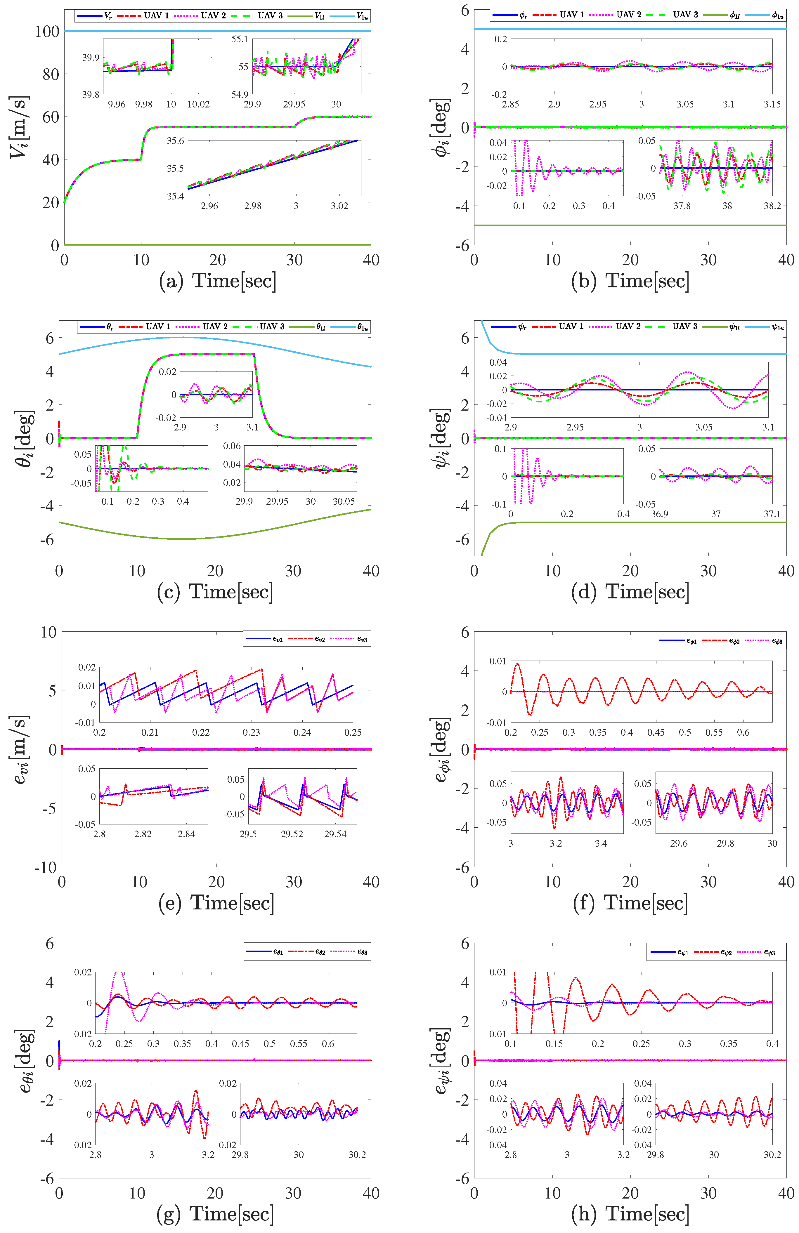
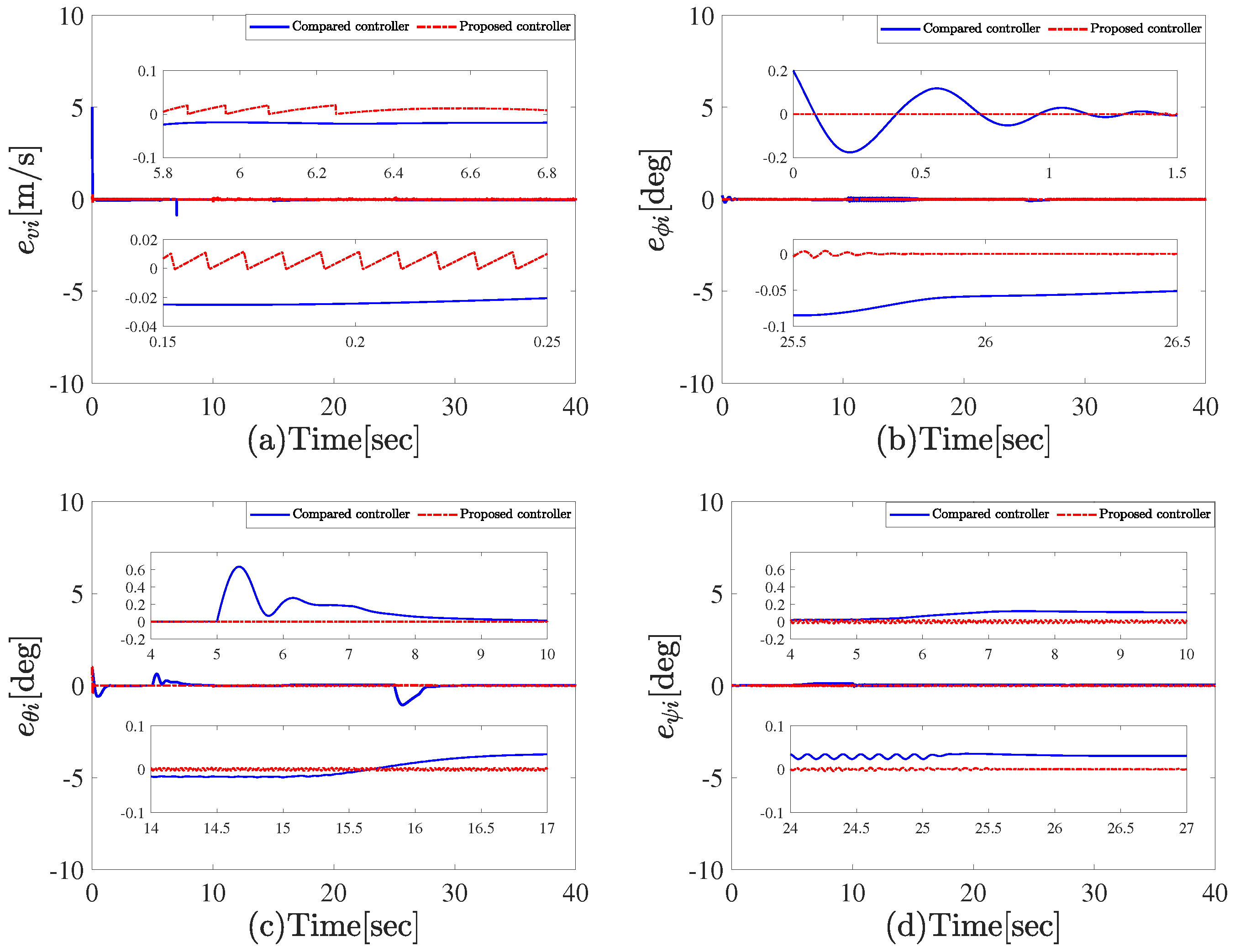
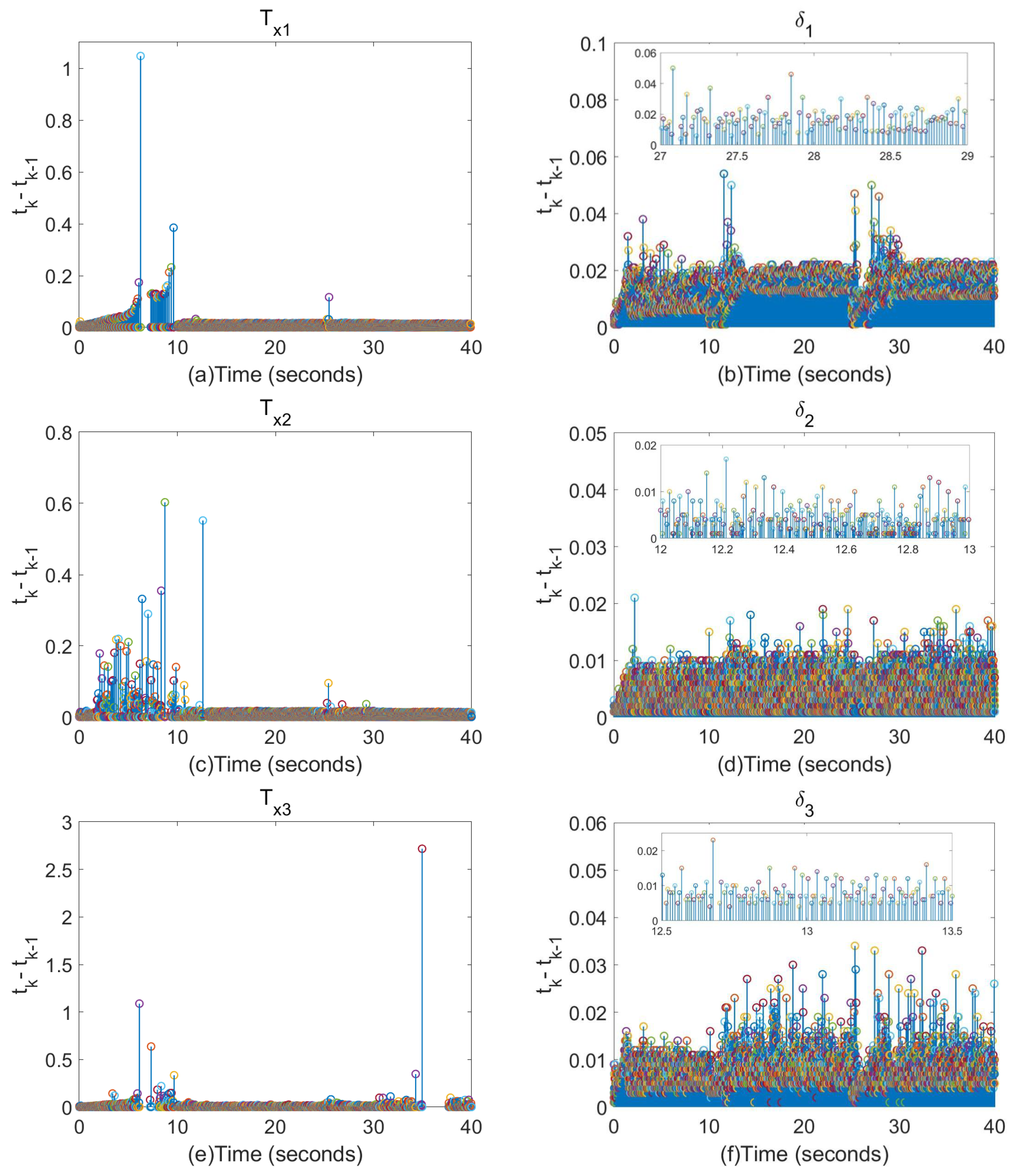
4. Simulation Results and Analysis

To validate the effectiveness of the proposed prescribed-time ETC scheme, this section conducts experimental verification. The parameters for each UAV are sourced from [43] and detailed in

Table 1. The parameter values of UAV.

Coefficient	Value	Unit	Coefficient	Value	Unit
$m_i$	20.64	kg	$c_{lpi}$	−0.213	${\mathrm{rad}}^{-1}·\mathrm{s}$
$b_i$	1.96	m	$c_{mqi}$	−3.449	${\mathrm{rad}}^{-1}·\mathrm{s}$
${\overline{c}}_i$	0.76	$\mathrm{m}$	$c_{npi}$	−0.151	${\mathrm{rad}}^{-1}·\mathrm{s}$
$S_i$	1.37	${\mathrm{m}}^2$	$c_{lri}$	0.114	${\mathrm{rad}}^{-1}·\mathrm{s}$
g	9.8	$\mathrm{m}·{\mathrm{s}}^{-2}$	$c_{nri}$	−0.195	${\mathrm{rad}}^{-1}·\mathrm{s}$
$\rho$	1.29	$\mathrm{kg}·{\mathrm{m}}^{-3}$	$c_{l{\delta }_{ai}}$	−0.056	${\mathrm{rad}}^{-1}$
$J_{xi}$	1.607	$\mathrm{kg}·{\mathrm{m}}^2$	$c_{n{\delta }_{ai}}$	−0.036	${\mathrm{rad}}^{-1}$
$J_{yi}$	7.51	$\mathrm{kg}·{\mathrm{m}}^2$	$c_{L{\alpha }_i}$	0.25	${\mathrm{rad}}^{-1}$
$J_{zi}$	7.18	$\mathrm{kg}·{\mathrm{m}}^2$	$c_{Y{\beta }_i}$	−0.1	${\mathrm{rad}}^{-1}$
$J_{xzi}$	0.59	$\mathrm{kg}·{\mathrm{m}}^2$	$c_{l{\beta }_i}$	−0.038	${\mathrm{rad}}^{-1}$
$c_{L0i}$	0.1	/	$c_{l{\delta }_{ri}}$	0.014	${\mathrm{rad}}^{-1}$
$c_{D0i}$	0.5	/	$c_{m{\alpha }_i}$	−0.473	${\mathrm{rad}}^{-1}$
$c_{l0i}$	−0.001	/	$c_{m{\delta }_{ei}}$	−0.364	${\mathrm{rad}}^{-1}$
$c_{m0i}$	0.022	/	$c_{n{\beta }_i}$	0.036	${\mathrm{rad}}^{-1}$
$c_{n0i}$	0.022	/	$c_{n{\delta }_{ri}}$	−0.055	${\mathrm{rad}}^{-1}$

. The communication topology is illustrated in Figure 1, while the initial states are presented in

Table 2. Initial states of UAVs.

	UAV1	UAV2	UAV3
x (m)	−20	10	30
y (m)	−10	10	−10
z (m)	100	100	100
V (m/s)	20	19.5	20
$\varphi$ ($°$)	0	−0.5	0
$\theta$ ($°$)	1	0.5	0
$\psi$ ($°$)	0	0.5	0
l (rad/s)	0	0	0
q (rad/s)	0	0	0
j (rad/s)	0	0	0

. Throughout the flight, the UAVs experience external disturbances represented as $d_{v1}=d_{v2}=d_{v3}={[0.25sin\left(t\right),0.4cos\left(2t\right),0.3cos\left(t\right)]}^{\mathrm{T}}$, $d_{\omega 2}=d_{\omega 3}={[0.3cos\left(2t\right),0.5sin\left(2t\right),0.25sin\left(t\right)]}^{\mathrm{T}}$.

The reference command for velocity and attitude subsystems are given as

$$\begin{array}{c}\hfill V_d=\left\{\begin{array}{c}20+{\displaystyle \frac{20}{s+1}},0s<t\le 10s,\hfill \\ 20+{\displaystyle \frac{35}{0.4s+1}},10s<t\le 30s,\hfill \\ 20+{\displaystyle \frac{40}{2s+1}},30s<t\le 40s,\hfill \end{array}\right.\end{array}$$

$$\begin{array}{c}\hfill {\mathit{\phi }}_d=\left\{\begin{array}{c}{[0,0,0]}^{\mathrm{T}},0s<t\le 10s,\hfill \\ {[0,0,0]}^{\mathrm{T}},10s<t\le 25s,\hfill \\ {[0,0,0]}^{\mathrm{T}},25s<t\le 40s,\hfill \end{array}\right.\end{array}$$

The time-varying state-constrained functions are set as: $0<V_i\le 100$, $-5<{\varphi }_{1i}\le 5$, $-12.5<{\varphi }_{2i},{\varphi }_{3i}\le 12.5$, $-5-sin\left(0.1t\right)<{\theta }_{1i}\le 5+sin\left(0.1t\right)$, $-10-sin\left(0.1t\right)<{\theta }_{2i},{\theta }_{3i}\le 10+sin\left(0.1t\right)$, $-5e^{-t}-5<{\psi }_{1i}\le 5e^{-t}+5$, $-15e^{-t}-5<{\psi }_{2i},{\psi }_{3i}\le 15e^{-t}+5$.

The designed parameters specified in (33)–(35), (60)–(63), (65) and (66) are set as follows: $a_1=0.6$, $a_2=1$, $\mu =0.13$, $T_c=3$, $k_{111}=k_{121}=20$, $k_{121}=k_{122}=20(t\in (0,10])$, $k_{121}=k_{122}=15(t\in (10,40])$, $k_{113}=k_{123}=20$, $\varsigma =0.1$, ${\gamma }_{vi}=10$, ${\chi }_{vi}=0.15$, ${\mathit{k}}_{211}={\mathit{k}}_{221}=\mathrm{diag}\{5,5,5\}$, ${\mathit{k}}_{212}=\mathrm{diag}\{10,10,10\}$, ${\mathit{k}}_{222}=\mathrm{diag}\{15,15,15\}$, ${\mathit{k}}_{213}={\mathit{k}}_{223}=\mathrm{diag}\{5,5,5\}$, $T_f=1$, $a_3=0.5$, $a_4=1$, ${\mathit{k}}_{311}={\mathit{k}}_{321}=\mathrm{diag}\{20,25,25\}$, ${\mathit{k}}_{312}={\mathit{k}}_{322}=\mathrm{diag}\{5,5,5\}$, ${\mathit{k}}_{313}={\mathit{k}}_{323}=\mathrm{diag}\{55,55,55\}$, ${\gamma }_{\omega 1}={\gamma }_{\omega 2}={\gamma }_{\omega 3}=\mathrm{diag}\{0.25,0.25,0.25\}$, ${\chi }_{\omega 11}=\mathrm{diag}\{1,0.01,0.01\}$, ${\chi }_{\omega 12}=\mathrm{diag}\{0.01,0.01,0.01\}$, ${\chi }_{\omega 12}=\mathrm{diag}\{1,1,0.01\}$, ${\eta }_{\omega 1}={\eta }_{\omega 2}={\eta }_{\omega 3}=0.001$, ${\chi }_{\omega 21}={\chi }_{\omega 22}={\chi }_{\omega 23}=0.5$, ${\chi }_{\omega 31}={\chi }_{\omega 32}={\chi }_{\omega 33}=0.5$.

The simulation results are presented in Figure 2, Figure 3, Figure 4 and Figure 5. Figure 2a–d demonstrate successful speed and attitude synchronization tracking, confirming the effectiveness of the proposed control methods. Additionally, the trajectories of speed and attitude adhere to the state constraints. Furthermore, the prescribed-time leader–follower consensus is achieved within 0.6 s, as illustrated in Figure 2e–h, indicating that $T\le T_c$, even in the presence of external disturbances. Figure 3 shows that the proposed mechanism effectively tracks the reference trajectories while adhering to state constraints, demonstrating superior control performance compared to the controller in [52]. From Figure 4a–f, we observe the time intervals of $T_{xi}$ and ${\delta }_i$ for each UAV. Finally, Figure 5 and

Table 3. The number of data transmission under different controllers.

Control Schemes	${\mathit{T}}_{\mathit{x}1}$	${\mathit{\delta }}_1$
Compared controller 1	40,000	40,000
Compared controller 2	21,059	6222
Proposed controller	5698	3231

reveal that, compared to the periodically sampled control (Controller 1) and static event-triggering control as described in [53] (Controller 2), the proposed controller significantly reduces the number of triggered events while exhibiting no Zeno behavior.

5. Conclusions

This paper has developed event-triggered prescribed-time synchronization strategies for velocity and attitude-tracking control of 6-DOF UAVs with state constraints. To avoid the need for infinite derivatives, a novel prescribed-time filter has been designed. The issue of asymmetric time-varying state constraints is addressed using a nonlinear state-transition function. Additionally, event-triggered mechanisms are separately designed for the velocity and attitude subsystems, effectively reducing communication and computational burdens. The simulation results demonstrate the effectiveness of the proposed control methods. However, real-world variations such as wind disturbances [54], sensor noise [55] can have an impact on tracking control for multiple UAVs, and these factors need to be considered as well. Future work will involve incorporating wind disturbances and sensor noise into the prescribed-time ETC framework, as well as considering switching topologies for further enhancements.

References

1. Doukhi, O.; Lee, D.J. Neural network-based robust adaptive certainty equivalent controller for quadrotor UAV with unknown disturbances. Int. J. Control Autom. Syst. 2019, 17, 2365–2374. [Google Scholar] [CrossRef]
2. Guerrero-Sánchez, M.E.; Hernández-González, O. Dynamics and control of UAVs. Machines 2024, 12, 749. [Google Scholar] [CrossRef]
3. Liu, H.; Meng, Q.; Peng, F.; Lewis, F.L. Heterogeneous formation control of multiple UAVs with limited-input leader via reinforcement learning. Neurocomputing 2020, 412, 63–71. [Google Scholar] [CrossRef]
4. Xiao, J.; Yuan, G.; Xue, Y.; He, J.; Wang, Y.; Zou, Y.; Wang, Z. A deep reinforcement learning based distributed multi-UAV dynamic area coverage algorithm for complex environment. Neurocomputing 2024, 595, 127904. [Google Scholar] [CrossRef]
5. Ahmed, Z.; Xiong, X. Adaptive impedance control of multirotor UAV for accurate and robust path following. Machines 2024, 12, 868. [Google Scholar] [CrossRef]
6. Lv, M.; Wang, N. Distributed control for uncertain multi-agent systems with the powers of positive-odd mumbers: A low-complexity design approach. IEEE Trans. Autom. Control 2023, 69, 434–441. [Google Scholar] [CrossRef]
7. Shi, Y.; Li, J.; Lv, M.; Wang, N.; Zhang, B. Distributed consensus control for 6-DOF fixed-wing multi-UAVs in asynchronously switching topologies. IEEE Trans. Veh. Technol. 2024, 1–15. [Google Scholar] [CrossRef]
8. Jackson, B.; Howell, T.; Shaha, K.; Schwager, M.; Manchester, Z. Scalable cooperative transport of cable-suspended loads with UAVs using distributed trajectory optimization. IEEE Robot. Autom. Lett. 2020, 5, 3368–3374. [Google Scholar] [CrossRef]
9. He, H.; Yuan, W.; Chen, S.; Jiang, X.; Yang, F.; Yang, J. Deep reinforcement learning-based distributed 3D UAV trajectory design. IEEE Trans. Commun. 2024, 72, 3736–3751. [Google Scholar] [CrossRef]
10. Fu, C.; Tian, Y.; Huang, H.; Zhang, L.; Peng, C. Finite-time trajectory tracking control for a 12-rotor unmanned aerial vehicle with input saturation. Isa Trans. 2018, 81, 52–62. [Google Scholar] [CrossRef]
11. Wang, D.; Zong, Q.; Tian, B.; Lu, H.; Wang, J. Adaptive finite-time reconfiguration control of unmanned aerial vehicles with a moving leader. Nonlinear Dyn. 2018, 95, 1099–1116. [Google Scholar] [CrossRef]
12. Sun, P.; Zhu, B.; Zou, Z.; Basin, M. Vision-based finite-time uncooperative target tracking for UAV subject to actuator saturation. Automatica 2021, 130, 109708. [Google Scholar] [CrossRef]
13. Huang, D.; Huang, T.; Qin, N.; Li, Y.; Yang, Y. Finite-time control for a UAV system based on finite-time disturbance observer. Aerosp. Sci. Technol. 2022, 129, 107825. [Google Scholar] [CrossRef]
14. Lin, G.; Li, H.; Ahn, C.; Yao, D. Event-Based finite-time neural control for human-in-the-loop UAV attitude systems. IEEE Trans. Neural Networks Learn. Syst. 2023, 34, 10387–10397. [Google Scholar] [CrossRef]
15. Zhou, S.; Guo, K.; Yu, X.; Guo, L.; Xie, L. Fixed-Time observer based safety control for a quadrotor UAV. IEEE Trans. Aerosp. Electron. Syst. 2021, 57, 2815–2825. [Google Scholar] [CrossRef]
16. Tao, M.; Chen, Q.; He, X.; Xie, S. Fixed-time filtered adaptive parameter estimation and attitude control for quadrotor UAVs. IEEE Trans. Aerosp. Electron. Syst. 2022, 58, 4135–4146. [Google Scholar] [CrossRef]
17. Lv, M.; Ahn, C.; Zhang, B.; Fu, A. Fixed-Time antisaturation cooperative control for networked fixed-wing unmanned aerial vehicles considering actuator failures. IEEE Trans. Aerosp. Electron. Syst. 2023, 59, 8812–8825. [Google Scholar] [CrossRef]
18. Zhou, Y.; Dong, W.; Liu, Z.; Lv, M.; Zhang, W.; Chen, Y. IBLF-based fixed-time fault-tolerant control for fixed-wing UAV with guar-anteed time-varying state constraints. IEEE Trans. Veh. Technol. 2023, 72, 4252–4266. [Google Scholar] [CrossRef]
19. Zhao, S.; Zheng, J.; Yi, F.; Wang, X.; Zuo, Z. Exponential predefined time trajectory tracking control for fixed-wing UAV with input saturation. IEEE Trans. Aerosp. Electron. Syst. 2024, 60, 6406–6419. [Google Scholar] [CrossRef]
20. Sun, F.; Zhang, J. Event-triggered prescribed-time tracking control for nonlinear systems with asynchronous switching. IEEE Trans. Circuits Syst. 2023, 70, 4159–4168. [Google Scholar]
21. Dong, T.; Chai, R.; Yao, F.; Tsourdos, A.; Chai, S.; Garcia, M. Terminal sliding mode attitude tracking control for unmanned vehicle with predefined-time stability. Aerosp. Sci. Technol. 2023, 142, 108669. [Google Scholar] [CrossRef]
22. Benaddy, A.; Labbadi, M.; Boubaker, S.; Alsubaei, F.; Bouzi, M. Predefined-time fractional-order tracking control for UAVs with pertur-bation. Mathematics 2023, 11, 4886. [Google Scholar] [CrossRef]
23. Li, Q.; Chen, Y.; Liang, K. Predefined-time formation control of the quadrotor-UAV cluster’ position system. Appl. Math. Model. 2023, 116, 45–64. [Google Scholar] [CrossRef]
24. Sun, P.; Zhu, B.; Li, S. Vision-based prescribed performance control for UAV target tracking subject to actuator saturation. IEEE Trans. Intell. Veh. 2024, 9, 2382–2389. [Google Scholar] [CrossRef]
25. Yang, S.; Pan, Y.; Cao, L.; Chen, L. Predefined-time fault-tolerant consensus tracking control for multi-UAV systems with prescribed per-formance and attitude constraints. IEEE Trans. Aerosp. Electron. Syst. 2024, 60, 4058–4072. [Google Scholar] [CrossRef]
26. Wang, F.; Gao, H.; Wang, K.; Zhou, C.; Zong, Q.; Hua, C. Disturbance observer-based finite-time control design for a quadrotor UAV with external disturbance. IEEE Trans. Aerosp. Electron. Syst. 2021, 57, 834–847. [Google Scholar] [CrossRef]
27. Mofid, O.; Mobayen, S. Adaptive finite-time backstepping global sliding mode tracker of quad-rotor UAVs under model uncertainty, wind Perturbation, and input Saturation. IEEE Trans. Aerosp. Electron. Syst. 2022, 58, 140–151. [Google Scholar] [CrossRef]
28. Han, Q.; Liu, Z.; Su, H.; Liu, X. Filter-based disturbance observer and adaptive control for euler–lagrange systems with application to a quadrotor UAV. IEEE Trans. Ind. Electron. 2023, 70, 8437–8445. [Google Scholar] [CrossRef]
29. Wang, H.; Li, M.; Zhang, H.; Liu, S. Predefined-Time Composite Adaptive Fuzzy Nonsingular Attitude Control for Multi-UAVs. IEEE Trans. Fuzzy Syst. 2024, 32, 6891–6903. [Google Scholar] [CrossRef]
30. Bemporad, A. Reference governor for constrained nonlinear systems. IEEE Trans. Autom. Control 1998, 43, 415–419. [Google Scholar] [CrossRef]
31. Dehaan, D.; Guay, M. Extremum-seeking control of statecon-strained nonlinear systems. IFAC Proc. Vol. 2004, 37, 663–668. [Google Scholar] [CrossRef]
32. He, W.; Yin, Z.; Sun, C. Adaptive neural network control of a marine vessel with constraints using the asymmetric barrier Lyapunov function. Math. Probl. Eng. 2016, 47, 1641–1651. [Google Scholar] [CrossRef] [PubMed]
33. Chang, X.; Wang, K.; Chen, K.; Fu, W. Full-state-constrained adaptive control for a class of UAVs suffering from coupled uncertainties using the HOBLF. Automatica 2021, 2021, 9963426. [Google Scholar] [CrossRef]
34. Ma, R.; Fu, L.; Fu, J. Prescribed-time tracking control for nonlinear systems with guaranteed performance. Automatica 2022, 146, 110573. [Google Scholar] [CrossRef]
35. Cao, Y.; Song, Y.; Wen, C. Practical tracking control of perturbed uncertain nonaffine systems with full state constraints. Automatica 2019, 110, 108608. [Google Scholar] [CrossRef]
36. Kazemy, A.; Lam, J.; Zhang, X. Event-triggered output feedback synchronization of master–slave neural networks under deception attacks. IEEE Trans. Neural Networks Learn. Syst. 2022, 33, 952–961. [Google Scholar] [CrossRef] [PubMed]
37. Zhang, X.; Han, Q.; Zhang, B.; Ge, X.; Zhang, D. Accumulated-state-error-based event-triggered sampling scheme and its application to H∞ control of sampled-data systems. Sci. China 2024, 67, 162206. [Google Scholar] [CrossRef]
38. Tian, B.; Cui, J.; Lu, H.; Liu, L.; Zong, Q. Attitude control of UAVs based on event-triggered supertwisting algorithm. IEEE Trans. Ind. Inf. 2021, 17, 1029–1038. [Google Scholar] [CrossRef]
39. Wang, J.; Bi, C.; Wang, D.; Kuang, Q.; Wang, C. Finite-time distributed event-triggered formation control for quadrotor UAVs with experimentation. ISA Trans. 2022, 126, 585–596. [Google Scholar] [CrossRef]
40. Wang, H.; Shan, J. Fully distributed event-triggered formation control for multiple quadrotors. IEEE Trans. Ind. Electron. 2023, 70, 12566–12575. [Google Scholar] [CrossRef]
41. Ma, C.; Zheng, S.; Xu, T.; Ji, Y. Finite-time asynchronous event-triggered formation of UAVs with semi-markov-type topologies. Sensors 2022, 22, 4529. [Google Scholar] [CrossRef] [PubMed]
42. Wang, F.; He, S.; Zhou, C.; Gao, Y.; Zong, Q. Distributed practical finite-time formation control of quadrotor UAVs based on finite-time event-triggered disturbance observer. IEEE Syst. J. 2023, 18, 355–366. [Google Scholar] [CrossRef]
43. Zhang, B.; Sun, X.; Liu, S.; Lv, M.; Deng, X. Event-triggered adaptive fault-tolerant synchronization tracking control for multiple 6-DOF fixed-Wing UAVs. IEEE Trans. Veh. Technol. 2022, 71, 148–161. [Google Scholar] [CrossRef]
44. Castaneda, H.; Salas-Pena, O.S.; Leon-Morales, J. Extended observer based on adaptive second order sliding mode control for a fixed wing UAV. ISA. Trans. 2017, 66, 226–232. [Google Scholar] [CrossRef]
45. Wu, C.; Yan, J.; Shen, J.; Wu, X.; Xiao, B. Predefined-time attitude stabilization of receiver aircraft in aerial refueling. IEEE Trans. Circ. Syst.-II Express Briefs 2021, 68, 3321–3325. [Google Scholar] [CrossRef]
46. Zhou, Z.; Tie, L. A new class of finite-time nonlinear consensus protocols for multi-agent systems. Int. J. Control 2014, 87, 363–370. [Google Scholar]
47. Wang, H.; Zhu, Q. Adaptive output feedback control of stochastic nonholonomic systems with nonlinear parameterization. Automatica 2018, 98, 247–255. [Google Scholar] [CrossRef]
48. Sun, J.; Yi, J.; Pu, Z. Fixed-time adaptive fuzzy control for uncertain nonstrict-feedback systems with time-varying onstraints and input saturations. IEEE Trans. Fuzzy Syst. 2011, 30, 1114–1128. [Google Scholar] [CrossRef]
49. Wang, C.; Lin, Y. Decentralized adaptive tracking control for a class of interconnected nonlinear time-varying systems. Automatica 2015, 54, 16–24. [Google Scholar] [CrossRef]
50. Yang, H.; Ye, D. Adaptive fixed-time bipartite tracking consensus control for unknown nonlinear multi-agent systems: An information classification mechanism. Inf. Sci. 2018, 459, 238–254. [Google Scholar] [CrossRef]
51. Zhou, N.; Kawano, Y.; Cao, M. Neural network-based adaptive control for spacecraft under actuator failures and input saturations. IEEE Trans. Neural Netw. Learn. Syst. 2020, 31, 3696–3710. [Google Scholar] [CrossRef] [PubMed]
52. Zhang, B.; Sun, X.; Lv, M.; Liu, S.; Li, L. Distributed adaptive fixed-time fault-tolerant control for multiple 6-dof uavs with full-state constraints guarantee. IEEE Syst. J. 2022, 16, 4792–4803. [Google Scholar] [CrossRef]
53. Sun, W.; Su, S.; Wu, Y.; Xia, J. Adaptive fuzzy event-triggered control for high-order nonlinear systems with prescribed performance. IEEE Trans. Cybern. 2022, 52, 2885–2895. [Google Scholar] [CrossRef]
54. Guo, K.; Jia, J.; Yu, X.; Guo, L.; Xie, L. Multiple observers based anti-disturbance control for a quadrotor UAV against payload and wind disturbances. Control Eng. Pract. 2020, 102, 104560. [Google Scholar] [CrossRef]
55. Chen, S.; Hu, F.; Chen, Z.; Wu, H. Correction method for UAV pose estimation with dynamic compensation and noise reduction using multi-sensor fusion. IEEE Trans. Consum. Electron. 2024, 70, 980–989. [Google Scholar] [CrossRef]
Figure 1. Communication topology.
Machines 13 00192 g001
Figure 2. The trajectory of speed and attitude and their tracking errors in proposed controller. (a) Speed response. (b) Roll−angle response. (c) Pitch−angle response. (d) Yaw−angle response. (e) Tracking error of speed. (f) Tracking error of roll angle. (g) Tracking error of pitch angle. (h) Tracking error of yaw angle.
Machines 13 00192 g002
Figure 3. Speed and attitude tracking response under comparative controller and proposed controller. (a) Speed response. (b) Roll−angle response. (c) Pitch−angle response. (d) Yaw−angle response.
Machines 13 00192 g003
Figure 4. Triggering time interval. (a) Data T x 1 . (b) Data δ 1 . (c) Data T x 2 . (d) Data δ 2 . (e) Data T x 3 . (f) Data δ 3 .
Machines 13 00192 g004
Figure 5. The number of times an event was triggered.
Machines 13 00192 g005