Abstract
Simultaneous Localization and Mapping (SLAM) has become a critical tool for fully autonomous driving. However, current methods suffer from inefficient data utilization and degraded navigation performance in complex and unknown environments. In this paper, an accurate and tightly coupled method of LiDAR-inertial odometry is proposed. First, a self-adaptive voxel grid filter is developed to dynamically downsample the original point clouds based on environmental feature richness, aiming to balance navigation accuracy and real-time performance. Second, keyframe factors are selected based on thresholds of translation distance, rotation angle, and time interval and then introduced into the factor graph to improve global consistency. Additionally, high-quality Global Navigation Satellite System (GNSS) factors are selected and incorporated into the factor graph through linear interpolation, thereby improving the navigation accuracy in complex and unknown environments. The proposed method is evaluated using KITTI dataset over various scales and environments. Results show that the proposed method has demonstrated very promising better results when compared with the other methods, such as ALOAM, LIO-SAM, and SC-LeGO-LOAM. Especially in urban scenes, the trajectory accuracy of the proposed method has been improved by 33.13%, 57.56%, and 58.4%, respectively, illustrating excellent navigation and positioning capabilities.
1. Introduction
Nowadays, vision-based and LiDAR-based methods are widely used in the field of Simultaneous Localization and Mapping (SLAM). Although cameras are cost-effective and provide rich visual information, their performance is highly susceptible to lighting variations, such as overexposure, underexposure, and rapid illumination changes, which are common in real-world driving scenarios [1,2,3]. In contrast, LiDAR sensors are invariant to lighting conditions and directly capture geometric structure through dense point clouds, enabling more reliable and accurate environmental perception under diverse illumination [4,5,6,7]. This fundamental difference in sensing modalities makes LiDAR a more robust choice for SLAM in unstructured or dynamically lit environments.
In autonomous driving, SLAM serves as the foundation for accurate path generation and localization: localization provides the vehicle with precise and continuous pose information within the global map, while path generation leverages this spatial information to plan feasible trajectories for path-tracking controllers [8]. Therefore, an accurate and stable SLAM system directly determines the reliability and accuracy of autonomous driving. In fully autonomous driving, LiDAR data is often fused with sensor data from IMU and GNSS to enhance localization accuracy. To support this, various methods have been proposed to optimize point cloud processing and multi-sensor fusion architectures [9,10]. Zhang et al. [11] proposed the LiDAR Odometry and Mapping (LOAM) method that associates the global map with the edge and planar features of the point clouds, and it established a fundamental framework for large-scale scenario SLAM. Based on LOAM, Shan et al. [12] proposed the Lightweight and Ground-Optimized LiDAR Odometry and Mapping (LeGO-LOAM) algorithm, which is designed for embedded systems with real-time capability. It also incorporates ground separation, point cloud segmentation, and improved Levenberg–Marquardt (L-M) optimization to enhance ground-awareness. In order to improve the speed and accuracy of loop closure detection, Kim et al. [13] proposed the Scan Context global descriptor that generates non-histogram features based on 3D LiDAR. By combining with LeGO-LOAM, it significantly boosts the efficiency of loop closure detection and enhances the global consistency of the map. Although it does not directly improve short-distance relative positioning accuracy, the global feature description framework it constructs lays the foundation for multi-sensor information fusion. Afterward, Shan et al. [14] proposed the LiDAR Inertial Odometry via Smoothing and Mapping (LIO-SAM) algorithm. This approach employs factor graphs as its back-end optimization scheme, enhancing the system’s robustness during rapid movements and demonstrating strong performance even under intense motion conditions.
In SLAM systems, original point clouds are typically downsampled to improve computational efficiency while preserving critical feature information. Zhang et al. [15] proposed the LILO system, which utilizes a uniform voxel grid filtering strategy and validated its performance in urban environments. Labbé et al. [16] developed the RTAB-Map library, which also uses voxel grids for downsampling and has achieved excellent performance in many outdoor long-term and large-scale datasets. The voxel grid filtering strategy employed in the above methods divides the original point clouds into fixed-size grids and represents each region using the centroid of its points. To address the limitations of using a single filter in complex scenes, Chen et al. [17] proposed the DLO method, which combines a Box filter with a voxel filter. The method was evaluated on the DAPA dataset and tested on an actual unmanned aerial vehicle system, demonstrating satisfactory performance. However, it remains challenging to achieve optimal results in scenes with varying levels of environmental feature richness. In response to this issue, Rakotosaona et al. [18] proposed a point cloud denoising network, PointCleanNet, which removes noise from original point clouds through end-to-end learning. Although this method can effectively downsample the original point clouds, the processing flow depends on GPUs, has high complexity and is struggles to satisfy the real-time needs of embedded systems. Therefore, studying an adaptive downsampling method that balances efficiency and real-time performance is of great importance.
In different motion scenes, autonomous vehicles exhibit varying motion characteristics, with their position and attitude continuously changing. Therefore, developing effective keyframe selection strategies is essential for extracting high-quality keyframes from diverse motion patterns across different scenes. When in underground environments, Kim et al. [19] designed a keyframe selection strategy that can dynamically adjust the keyframe selection interval. This strategy is primarily used to select sparse or dense keyframes based on the number of downsampled points in spacious or confined underground environments. Schöps et al. [20] proposed the BAD SLAM algorithm that adopts a keyframe selection strategy based on the interval of original point cloud frames. But in fast-moving scenes, it may face the problems of insufficient keyframes due to the single screening condition. To address this issue, Nguyen et al. [21] put forward the MILIOM algorithm which uses the position translation and rotation angle as the thresholds to screen keyframes. However, in scenes where objects are moving slowly or stationary, this strategy may result in inaccurate keyframe selection. Hu et al. [22] proposed a keyframe selection method based on the Wasserstein distance, which assesses frame importance by comparing the Gaussian mixture model (GMM) distributions of point clouds. However, this keyframe selection method inevitably introduces additional computation time. Shen et al. [23] proposed an adaptive method based on the semantic difference between frames, and it has a better positioning accuracy than the algorithms that mainly use geometric features as the criterion. However, the misclassification of semantic segmentation labels may lead to calculation deviations of the KL divergence, resulting in the wrong selection of keyframes.
At present, LiDAR is typically used in conjunction with other sensors, such as Inertial Measurement Unit (IMU) and Global Navigation Satellite System (GNSS), for state estimation and mapping [24,25,26,27,28]. In complex unknown environments, multi-sensor fusion technology has been demonstrated to significantly enhance navigation accuracy. Li et al. [29] proposed the GIL framework, which tightly integrates GNSS Precise Point Positioning (PPP), Inertial Navigation System (INS), and LiDAR, achieving over 50% reduction in positioning errors in partially occluded scenes. Chiang et al. [30] demonstrated that integrating Normal Distribution Transform (NDT) scan matching with Fault Detection and Exclusion (FDE) mechanisms can effectively constrain pose drift in GNSS-denied environments. With INS/GNSS initialization, the system achieved lane-level accuracy (0.5 m), further supporting the necessity of multi-sensor fusion. Building on this idea, Chen et al. [31] proposed GIL-CKF, a GNSS/IMU/LiDAR fusion method that combines filtering with graph optimization. It incorporates a scenario optimizer based on GNSS quality metrics, allowing GNSS and motion state observations to alternate with IMU data in an EKF framework, thereby improving navigation accuracy. In parallel, Hua et al. [32] incorporated motion manifold constraints, further enhancing the system’s robustness in degraded motion scenes. As the measurement from GNSS is unreliable from time to time, the inaccurate GNSS factor can even have a negative influence on the accuracy of trajectory estimation. For outliers in the aided velocity information provided by GNSS, Lyu et al. [33,34] proposed a class of robust moving base alignment method, and the residual is used to reconstruct the observation vector to detect and isolate these outliers. The above work studied multi-sensor fusion and GNSS outlier suppression and achieved good results. However, more research is needed on how to select high-quality GNSS factors and on aligning them with LiDAR keyframe timestamps.
To overcome the above limitations, this paper puts forward a tightly coupled LiDAR–inertial odometry method for autonomous driving, based on a self-adaptive filter and factor graph optimization. The main contributions of this paper are as follows:
- Aiming at the limitations of traditional voxel grid filters, a self-adaptive voxel grid filter is proposed that dynamically downsamples point clouds based on environmental feature richness. This filter adaptively adjusts the voxel grid size based on the density and geometric features of the original point clouds, thus effectively balancing navigation accuracy and real-time performance of the autonomous vehicles.
- To make full use of point cloud frames, a multi-parameter joint keyframe selection strategy is proposed. This strategy uses the cumulative translational displacement, cumulative rotation angle, and time interval between adjacent frames as screening thresholds. Through joint screening with multiple thresholds, this strategy can capture the motion data of the autonomous vehicles in different scenes more accurately.
- To improve the global optimization based on factor graph, an effective GNSS factor selection strategy is proposed. High-quality GNSS observations are selected, and they are aligned with the corresponding keyframes through linear interpolation. This mechanism makes full use of the absolute position signals of GNSS, thereby improving the navigation and positioning accuracy in complex environments.
2. Sensor Methods and Error Modeling
2.1. TOF LiDAR Ranging Method
The Time of Flight (TOF) principle, with its simple and accurate distance measurement capabilities, has become an important technical foundation for achieving position estimation and map construction. The point cloud data of the LiDAR used in this paper is collected based on this principle. The schematic diagram of TOF distance measurement is shown in Figure 1.
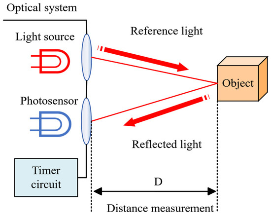
Figure 1.
TOF ranging schematic.
The TOF is to emit single-pulse or continuous-pulse laser through a laser emitter, and then the sensor receives the laser reflected by the target. Then, the distance between the LiDAR and the object can be calculated as follows:
where is the distance to the target; is the speed of light; is the number of clock pulses; and is the clock pulse frequency.
2.2. IMU Error Modeling
In an inertial navigation system, both the commanded angular rate and the gyroscope drift influence the resulting attitude angle errors. In addition, the drift of the gyroscope produces an extra angular deviation in the reverse direction. The attitude error model of the IMU can therefore be expressed within the navigation frame n as follows:
where is the platform attitude error calculated in the navigation frame; is the three-axis gyroscope random constant offset in the navigation frame; is the angular rates from the inertial frame to the navigation frame; and is the derivative of . In addition, can be represented as:
The attitude error model expressed in the ENU coordinate frame is given as follows:
where denotes the latitude; represents the radius of curvature in meridian; and denotes the radius of curvature in prime vertical.
The inertial navigation system utilizes the measurements provided by the inertial measurement unit to compute navigation information. The correlation between the accelerometer output and the carrier velocity can be characterized through the velocity error model, expressed in the navigation frame n as follows:
where is the rate error in the navigation frame; denotes the derivative of ; denotes the specific force vector in the navigation frame; represents the three-axis accelerometer bias in the navigation frame; is the earth’s rotation angular rate; is the derivative of ; represents the angular rate from the earth frame to the navigation frame; the corresponding relationships are given in Equations (8) and (9), respectively:
The velocity error equation can be represented as follows:
The position error equation can be represented as follows:
2.3. GNSS Error Modeling
Currently, there are four main global navigation satellite systems: the United States GPS, Russia’s GLONASS, China’s Beidou, and the European Union’s Galileo. In practical applications, users use satellite receivers to receive radio signals for real-time positioning and navigation.
The main error sources that affect GNSS measurement accuracy can be divided into three categories: (1) GNSS satellite errors, which mainly include satellite orbit errors, satellite clock errors, and ephemeris errors; (2) Signal propagation errors, which mainly include ionospheric errors and atmospheric delays caused by tropospheric errors, as well as multipath effects during signal propagation; (3) Receiver errors, mainly including receiver clock errors and receiver noise. The position error and velocity error of the GNSS receiver can be regarded as white noise or a first-order Markov process with a short correlation time and a small mean square error [28]. Therefore, it can be modeled as a first-order Markov process.
The GNSS position error model can be represented as follows:
where , , denote the latitude, longitude, and altitude errors of the GNSS receiver, respectively; , , are the Markov process correlation time, generally taken as ; , , are Gaussian white noise.
The GNSS velocity error model can be expressed as follows:
where , , denote the east, north, and up velocity errors of the GNSS receiver, respectively; , , are the Markov process correlation time, generally taken as ; , , are Gaussian white noise.
3. Tightly Coupled LiDAR–Inertial Odometry Framework
The proposed method, illustrated in Figure 2, comprises four major modules: the GNSS module, the Inertial Measurement Unit (IMU) module, the loop-closure detection module, and the LiDAR odometry module. Firstly, the IMU compensates for the motion distortion of the point clouds and provides the initial pose estimation for the LiDAR odometry. Thereafter, the LiDAR odometry matches the feature point clouds of the current frame with the submap. Then, by utilizing scan-context [13], the feature point clouds are encoded into point cloud descriptors to achieve efficient closed-loop detection [35]. The IMU pre-integration factor, the LiDAR odometer factor, the GNSS factor, and the loop closure factor are inserted into the global factor graph, and finally, global graph optimization is updated by the Bayes tree [36]. Benefiting from the multi-sensor fusion feature of factor graph optimization, this framework exhibits a certain level of robustness against transient sensor faults. When one sensor provides abnormal data, it can also help identify the faulty sensor source, and the continuous and consistent observations from other sensors can dominate the optimization process, thereby effectively suppressing the accumulation of errors and ensuring the system’s stability during the fault period. Compared with other traditional methods, the proposed approach aims to improve the accuracy of simultaneous localization and mapping for ground vehicles.
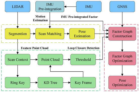
Figure 2.
Overall framework of the proposed approach.
3.1. Self-Adaptive Voxel Grid Filtering
Since there is a large amount of redundant data in the 3D LiDAR point clouds, an adaptive voxel grid downsampling strategy can be adopted. While retaining the characteristics of the point clouds, this strategy can significantly reduce the number of original point clouds, enabling the improvement of the computing speed of the subsequent point cloud registration program without sacrificing too much accuracy. The traditional voxel grid downsampling strategy divides the input original point clouds into three-dimensional voxel grids, taking the centroid of the points within each voxel to represent all the points it contains. The procedure is as follows:
The side length of the point cloud bounding box is calculated as:
where and are the side lengths of the point cloud bounding box in the directions of the x, y, and z axes, respectively; , , and , , are denoted as the maximum values and the minimum values on the three coordinate axes of each point cloud, respectively.
Then the point clouds are divided into voxel grids, the total number of which is . The calculation strategy is as follows:
where r is the side length of each grid voxel; are the number of grids on the x, y and z axes, respectively.
Finally, the index of each point in the voxel grid can be calculated as follows:
where and are the indices of a point in the voxel grid along the x, y and z axes, respectively; and is the overall index of the point in the voxel grid.
The elements are sorted according to their index values, and then the gravity of each voxel centroid is calculated. Finally, the points within each voxel grid are replaced with the centroid of that corresponding voxel grid.
It should be noted that the sizes and quantities of 3D point clouds collected by different scenes and LiDAR devices often vary. Therefore, the traditional voxel downsampling strategy proposed in [37] has to rely on adjusting the grid size manually [38]. However, this traditional voxel grid filter has certain deficiencies. In view of this, this paper proposes a new type of adaptive voxel grid filter to better address these problems. In scenes with abundant feature information, this filter reduces the side length of the voxel grid to retain as many feature point clouds as possible, thereby effectively improving the accuracy of subsequent registration approaches. In scenes with scarce feature information, it increases the side length of the voxel grid to filter out as many invalid point clouds as possible, thus accelerating the speed of subsequent point cloud registration. Based on the size and density of the original point clouds, the strategy can adaptively calculate the length of the voxel grid, making the number of point clouds basically remain between and after downsampling.
In the self-adaptive voxel grid filter proposed by this paper, the following conditions must be met one, of which for the end of one downsampling:
where is the edge length of the voxel grid that grows in each iteration; is the number of iterations; is the maximum number of iterations; is the self-adaptive voxel grid filtering function; is the maximum and minimum number of point clouds after downsampling.
The voxel side length can be calculated through the following steps. To calculate its initial value more accurately, the point cloud density is defined as:
where is point cloud density; is the number of point clouds before downsampling; and is the maximum range of the point cloud.
The length of the voxel grids calculated according to and are defined as:
where and are the length of the voxel grids calculated according to and ; is the initial length of the finally obtained voxel grid; a, b and c are adjustment coefficients.
In order to keep the number of points in the filtered point clouds stable within an appropriate range, construct an automatic feedback mechanism for adjusting the voxel grid. Denote the feedback error and the update formula for the side length of the voxel grid as follows:
where is the feedback gain; is current filtered point count; and is adjustment coefficient.
It should be noted that if the value of parameter is too small, numerous characteristics of the original point clouds will be lost. Conversely, if the value of parameter is too large, the number of point clouds after filtering will be excessively substantial, potentially resulting in insufficient computing resources. So suitable should be set by comprehensively considering the computing resources and the number of features.
The flow chart of downsampling is shown in Figure 3, and should be firstly calculated. After that, are calculated according to Equations (23)–(26). Then, these aforementioned parameters are substituted into the self-adaptive voxel grid filter. After downsampling, can be obtained, if is not within the interval and is less than , the length of voxel grid will be adapted according to Equations (27) and (28) and be substituted into the self-adaptive voxel filter again. Repeat the previous step until is within the interval or is greater than . Finally, the whole target point clouds will be output. Actually, iteratively calculating the voxel grid length is rather time-consuming. Given that the LiDAR usually operates at the same resolution, the adaptive voxel filter proposed in this paper calculates a suitable voxel grid length in the first frame and then directly applies it to subsequent downsampling processes. As long as the number of points in the downsampled point cloud remains within the range of during subsequent processing, the voxel grid size can remain unchanged, thereby saving computational resources.
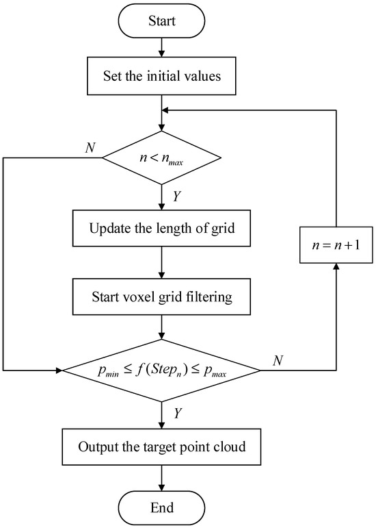
Figure 3.
Flow chart of self-adaptive voxel grid filter.
3.2. Multi-Criteria Keyframe Selection Strategy
In the proposed SLAM system, the data used to estimate the pose in the system includes IMU pre-integration, LiDAR odometry, GNSS measurements, and results of loop closure. The error of trajectory estimated by LiDAR odometry and the integral value of IMU will accumulate as the size of the map increases. Therefore, the backend global optimization module needs to be introduced to fuse and optimize the pose estimation of IMU and LiDAR. In this paper, the factor graph strategy is designed to realize global optimization. Flexibility is one characteristic of the factor graph strategy, which can fuse the state estimation of multiple sensors to obtain the final optimization result. Therefore, both pose estimation accuracy and overall map consistency can be improved. Even in scenes with poor GNSS signals, the high-quality keyframes selected by our strategy can maintain stable pose estimation by LiDAR feature matching data and IMU pre-integration information.
The proposed factor graph model is shown in Figure 4. Firstly, the pose transformation from the previous to the current frame is computed, and the LiDAR odometry factor is then constructed based on this result. Then, the IMU data is integrated to derive the pose of the unmanned vehicle [39], so that the IMU pre-integration factor can be constructed based on this pose and subsequently incorporated into the factor graph. At the same time, the loop-closure factor and GNSS factor are also incorporated into the factor graph to mitigate cumulative errors arising from prolonged operation.
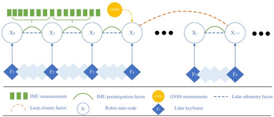
Figure 4.
The factor graph model of the proposed method.
In the Simultaneous Localization and Mapping (SLAM) system, the input frequency of the odometer is usually high. If all downsampled point cloud frames are directly added to the factor graph as keyframes without screening, a large number of variables to be optimized will impose a huge computational burden on the system, making it difficult for the system to run in real time. In addition, considering that when the unmanned vehicle makes a sharp turn, the odometer is prone to introducing nonlinear errors. Or when the vehicle is stationary but the surrounding environment changes dynamically, it will lead to a decrease in the repeatability of point cloud observations, both of which may increase the position error. Therefore, based on the traditional keyframe selection strategy that only uses the translation distance as the screening threshold, this paper proposes a new strategy: selecting keyframes through three indicators, namely the Euclidean distance, the change in the rotation angle, and the time interval. The pose transformation between two adjacent frames can be represented as
The magnitude of angle change is represented by the sum of rotational components as
The translational transformation of two adjacent point clouds is represented by Euclidean distance, which can be expressed as follows:
Therefore, the cumulative translational transformation and the cumulative rotation angle change can be calculated separately as follows:
where is the sequence number of the previous keyframe in the entire odometry output data; is the sequence number of the current odometry output data; is the new keyframe data; is the current odometry output data; is the cumulative translational transformation; is the cumulative rotation angle change; is the threshold of translational transformation; is the time interval; is the threshold of time interval; and is the threshold of rotation angle change.
When one of the preset thresholds of the keyframe selection strategy is met, the current frame is selected as a keyframe. According to the pose transformation of the keyframe, the odometry factor will be calculated and registered in the factor graph. At the same time, the current frame is registered to the global map to construct the global point cloud. After all the keyframes are selected, the odometry is calculated based on each frame of point cloud, but only the keyframes can participate in the global optimization. This strategy considerably reduces the amount of global calculation while ensuring that the accuracy of position estimation does not decline significantly. In addition, this strategy also takes into account the situation where the Euclidean distance changes little, but the rotation angle is large or the stationary time in a dynamic environment is too long. In this case, most feature points will vary, making it essential to designate this frame as a keyframe to fully leverage the environmental information.
3.3. GNSS Integration in Factor Graph Optimization
As shown in Figure 4, after adding high-quality GNSS factors to the factor graph, the accuracy of state estimation and mapping can be greatly improved, especially in long-duration and long-distance navigation tasks. On the other hand, inaccurate GNSS factors will have a negative impact on the optimization results of the entire factor graph. Therefore, after receiving GNSS signals, it is necessary to first screen out signals with higher credibility according to their accuracy flag bits. This high-quality GNSS factor selection mechanism is essentially an effective sensor fault detection method. By comparing the system-estimated position information with the received GNSS position information, it can proactively identify and exclude unreliable GNSS signals. Secondly, to improve the reliability of GNSS factors, this study draws on the latest achievements in the field of multi-sensor fusion [40] and proposes the improved GNSS factor strategy. By linearly interpolating to align the timestamps of GNSS and adjacent keyframes, the positioning error in dynamic environments is significantly reduced. When the GNSS signal is interrupted in GNSS-challenged environments such as urban canyons, tunnels, or dense forests, the combined constraints of IMU and LiDAR ensure system stability; the two sensors complement each other to compensate for the lack of GNSS absolute position constraints, preventing severe pose drift even during extended GNSS outages.
This paper proposes a method for selecting high-quality GNSS factors and linearly interpolating to align the timestamps. First, a GNSS observation is only incorporated as a factor if the received GNSS position falls within the estimated position range from the system’s LiDAR and IMU. Next, the LiDAR frame timestamp is compared against the GNSS signal timestamp. Only when the difference value between them is smaller than the preset threshold will linear interpolation be performed on GNSS measurements based on the timestamp. The interpolation process is as follows:
where are the weight factors of linear interpolations; are the timestamp of the keyframe and the timestamps of the two adjacent GNSS factors before and after it, respectively; , , represent the interpolated longitude, latitude, and altitude of GNSS factor, respectively; , , , and , , are the former and current longitude, latitude, and altitude of GNSS factor, respectively. In this way, the GNSS factor can be inserted into the factor graph, as illustrated in Figure 4.
4. Results and Analysis
4.1. Experimental Settings
Accurate ground truth is provided by a Velodyne LiDAR scanner (Velodyne LiDAR Inc., San Jose, CA, USA) and a GPS localization system (Oxford Technical Solutions Ltd., Oxford, UK). The Velodyne LiDAR scanner, with its high-precision scanning capabilities, can capture detailed three-dimensional information of the surrounding environment. The GPS localization system, on the other hand, offers precise positioning data, ensuring accurate determination of the vehicle’s location in real time. KITTI datasets are captured by driving around the mid-size city of Karlsruhe, in rural areas, and on highways. These diverse driving scenes allow for the collection of rich and comprehensive data. In the mid-size city of Karlsruhe, various urban features such as buildings, roads, and intersections are included. Rural areas provide natural landscapes and different terrains, while highways contribute to data under high-speed and long-distance driving conditions.
Based on KITTI dataset, a series of experiments were conducted to verify the validity of the proposed method. The experiments were carefully designed to test different aspects of the method, including its accuracy and efficiency. Multiple trials were carried out to ensure reliable and reproducible results. All the experiments were performed on a laptop equipped with an AMD Ryzen 4800U processor and 16 GB of RAM, running Ubuntu 18.04. The AMD Ryzen 4800U processor provides sufficient computing power to handle the complex algorithms and data processing required in the experiments. The 16 GB of RAM ensures smooth operation and the ability to manage large datasets without significant performance bottlenecks.
4.2. Test Results with Self-Adaptive Voxel Grid Filter
To verify the effectiveness of the strategy, the self-adaptive voxel grid filter is applied to point cloud dataset KITTI. is set to be , is set to be 0.01. Those point clouds shown in Figure 5 are collected in highway, town, and urban scenes.
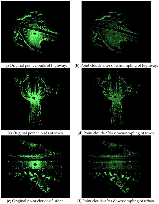
Figure 5.
Results of downsampling in highway, town and urban scenes.
The results of the adaptive voxel filter are shown in Figure 5, with the left figures (a), (c), (e) showing the original point clouds and the right figures (b), (d), (f) showing the point clouds after downsampling. Table 1 shows the quantity changes of the point clouds after downsampling.

Table 1.
Results after downsampling.
As is shown in Figure 5, using a self-adaptive voxel grid filter, without losing too many feature points, the data in the point clouds has been greatly decreased. The amount of point clouds in highway scene, town scene, and urban scene is down by 91.5%, 91.2%, and 90.8%, respectively. The substantial reduction of point cloud data boosts processing efficiency and eases computational burdens. Meanwhile, minimal loss of feature points retains key information for subsequent analysis. This balance between data reduction and feature preservation verifies the feasibility of the method, ensuring the efficiency and reliability of the adaptive filtering strategy proposed in this paper.
4.3. Results in Highway Scene
The proposed method was then verified for the accuracy of trajectory in a highway scene. Some snapshots of this scene and the real trajectory on the satellite image can be found in Figure 6. In order to reflect the superiority of the proposed method, it was compared with the prevalent SLAM methods such as Advanced Implementation of LOAM (ALOAM), LIO-SAM, and Scan Context-LeGO-LOAM (SC-LeGO-LOAM).
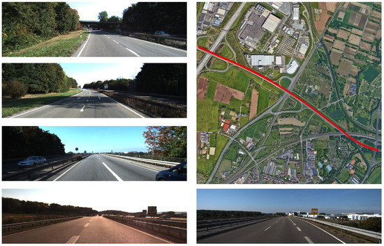
Figure 6.
Satellite image and some snapshots of the highway scene. The red line on the satellite image indicates the experimental trajectory.
Figure 7 shows the difference in trajectories between the proposed method, the methods for comparison, and the value of ground truth. It is observed that in the highway scene, the long-distance and long-duration movement increases the error accumulation of inertial sensors, thereby reducing the overall positioning accuracy of the SC-LeGO-LOAM and LIO-SAM methods. Moreover, since there is no actual loop closure in this scene and there are a large number of repetitive structures, loop closure detection strategies such as the scan context of these two algorithms are prone to being misled by similar structures and producing false matches. This also leads to a decrease in positioning accuracy and system stability. Instead, the ALOAM method, lacking a loop closure detection module, performs better than the previous two algorithms.
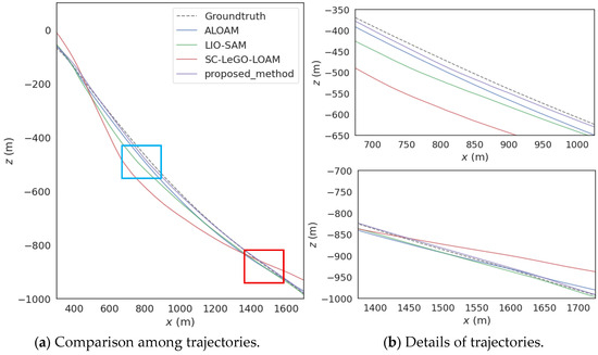
Figure 7.
Comparison among trajectories of highway scene.
In contrast, the adaptive voxel filtering strategy proposed here ensures that the number of downsampled point clouds obtained per frame remains within a stable range. This range is carefully designed to balance efficiency and accuracy while retaining necessary feature points. This reduces the probability of false matches of the loop closure detection strategy. Additionally, the key-frame selection strategy is improved to ensure that there are enough keyframes for pose estimation during high-speed movement. In addition, since there is no occlusion in this scene, the proposed algorithm significantly reduces the position error after incorporating GNSS factors.
To be more specific, as shown in Table 2, compared with ALOAM, LIO-SAM, and SC-LeGO-LOAM, the proposed method achieves an improvement of 18.43%, 62.84%, and 61.32% in trajectory accuracy, respectively. Compared with the town and urban scenes, the number of static feature points on highways is the smallest. Moreover, most of them are repetitive structures that can easily lead to misjudgments in the loop closure detection strategy, and there are also many dynamic feature points. Therefore, the position error of each algorithm in this scene is the largest.
Table 2.
Relative translation error for all methods in highway scene.
4.4. Results in Town Scene
Next, the proposed method was tested in a town scene. Some snapshots and the real trajectory of this experiment can be found in Figure 8.
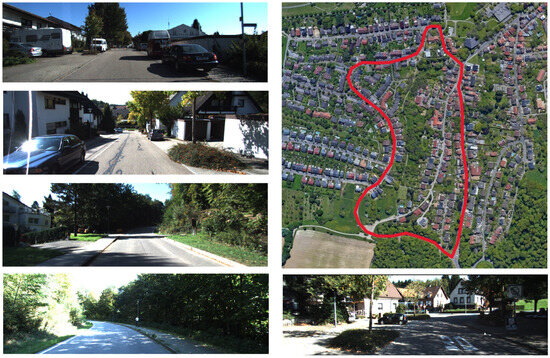
Figure 8.
Satellite image and some snapshots of the town scene. The red line on the satellite image indicates the experimental trajectory.
In Figure 9, Figure (b) corresponds to the blue frame and red frame in Figure (a). In the town scene, there are a large number of static features. The other three algorithms use a fixed grid side length for the voxel filtering strategy of the original point clouds. However, for the rich feature information in this scene, the default grid side length results in too many feature points being lost in the downsampled point clouds after voxel filtering, leading to a decrease in the position accuracy. The adaptive voxel filtering method proposed in this paper can dynamically decrease the size of the voxel grid side length according to the size and density of the original point clouds. Thus, the number of feature point clouds input to the next stage is maintained within a reasonable range, taking into account both the accuracy of position estimation and real-time performance.
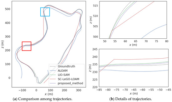
Figure 9.
Comparison among trajectories of the town scene.
In addition, this scene is also characterized by low speed, frequent turning, and the existence of loop closures. Therefore, based on the fact that ALOAM and SC-LEGO-LOAM only use the translation distance, and LIO-SAM adds the rotation angle as the key-frame selection strategy. The method proposed in this paper adopts a key-frame selection strategy that additionally incorporates a time threshold as the screening criterion. This strategy overcomes the problem of increased position estimation errors that may occur when stationary for a long time or turning slowly at intersections. Moreover, when passing through open intersections, the strategy proposed in this paper, which introduces high-quality GNSS factors into the factor graph optimization, can effectively reduce the positioning error.
Table 3 shows that compared with ALOAM, LIO-SAM and SC-LeGO-LOAM, the proposed method improves the positioning accuracy by 27.18%, 25.37%, and 31.19%, respectively. Since this scene has more static feature points compared to highway and urban scenes, and there are no large numbers of structures that may lead to misjudgments in loop closure detection, the position accuracy of each algorithm in this scene is the best.
Table 3.
Relative translation error for all methods in the town scene.
4.5. Results in Urban Scene
Finally, the proposed method was tested in an urban scene. Some snapshots and the real trajectory of this experiment are presented in Figure 10. In Figure 11, Figure (b) corresponds to the blue frame and red frame in Figure (a). In the urban scene, the static feature information is rich but unevenly distributed. For example, there are significant differences in the point cloud quantity between building clusters and open intersections. When downsampling the original point clouds, the fixed-side-length voxel filtering strategy adopted by ALOAM, LIO-SAM, and SC-LeGO-LOAM is difficult to achieve good results. When the feature information is abundant, some key feature point clouds will be lost, which in turn leads to relatively large errors in subsequent key-frame processing and position calculation. While when the feature information is scarce, too many feature points are collected. This not only fails to improve the accuracy but also slows down the speed at which the program processes the point clouds. However, the adaptive voxel filtering can effectively overcome the challenge of uneven distribution of static features. It dynamically adjusts the voxel grid size according to the size and density of the point clouds to ensure that the collected feature points are maintained within a reasonable range, so that the subsequent process can achieve accurate position estimation while also taking into account the processing speed.
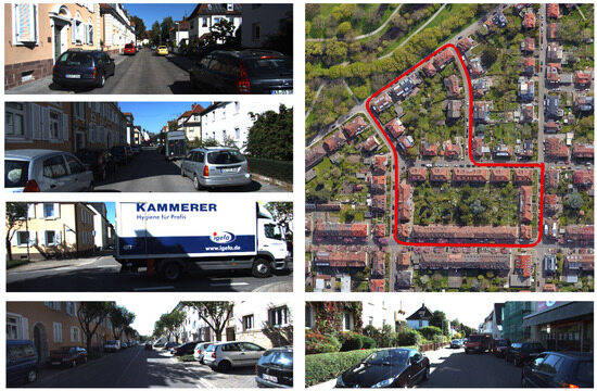
Figure 10.
Satellite image and some snapshots of the urban scene. The red line on the satellite image indicates the experimental trajectory.
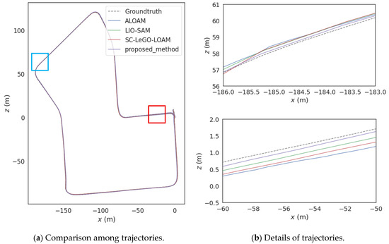
Figure 11.
Comparison among trajectories of the urban scene.
In addition, due to the characteristics of many sharp turns and occlusions in this scene, the improved key-frame selection strategy can collect a sufficient number of keyframes at turning points to achieve more accurate positioning. Even in environments where valid GNSS signals are lacking in most areas, the dense keyframes selected by this strategy still provide sufficient interframe motion constraints. These constraints are used to construct continuous factor graph edges, thereby suppressing cumulative pose errors. Moreover, high-quality GNSS factors can be screened out in the relatively small number of unobstructed areas and incorporated into the factor graph; these GNSS factors help optimize the global pose and reduce position errors caused by issues such as IMU drift or LiDAR mismatches.
Table 4 shows that compared with ALOAM, LIO-SAM and SC-LeGO-LOAM, the proposed method enhances the accuracy of the position by 33.13%, 57.56%, and 58.4%, respectively. Compared with the other two scenes, there are not many repetitive structures in the urban scene, but there are a considerable number of dynamic feature point clouds. Therefore, the performance of each algorithm in this scene is at an intermediate level among the three scenes.
Table 4.
Relative translation error for all methods in the urban.
In practical applications, real-time performance is another crucial indicator for evaluating SLAM systems. The runtime of ALOAM, LIO-SAM, SC-LeGO-LOAM, and the proposed method is tested on all three datasets, and the results are shown in Table 5.
Table 5.
Runtime of algorithms for processing one scan.
It can be seen that the runtime of the proposed method decreases by about 5.47% and 18.79%, respectively, when compared with ALOAM and LIO-SAM. In addition, it should be noted that SC-LeGO-LOAM adds the Scan Context algorithm to the lightweight LeGO-LOAM method to detect loop closures. In structured scenes without loop closures, such as highways, false detections are likely to occur. The proposed method has a slightly longer running time, but it can reduce the probability that the estimation accuracy is reduced due to false loop-closure detections.
5. Conclusions
SLAM systems suffer from the challenges of instability and inaccuracy. In this paper, a new method is designed to perform real-time and accurate state estimation for fully autonomous driving. The proposed method adopts an adaptive voxel grid filter, which dynamically adjusts the voxel grid size in scenes with different feature information richness levels to ensure both accuracy and real-time performance. The strategy to select keyframes can help the system to be more accurate in various scenes. At the same time, the GNSS factor can correct the trajectory and effectively reduce the position error over time. Experimental results indicate that the proposed approach operates efficiently across various scenes while yielding smaller position errors. The proposed method has demonstrated very promising results when compared with the other methods, such as ALOAM, LIO-SAM, and SC-LeGO-LOAM. Especially in urban scenes, the trajectory accuracy of the proposed method achieves improvements of 33.13%, 57.56%, and 58.4%, respectively.
In the future, the deep-learning method can be applied to the proposed method to remove the dynamic objects. In addition, the visibility-based range image method and the LiDAR method can be fused to get better accuracy.
Author Contributions
Conceptualization, W.L.; formal analysis, X.T. and Z.D.; funding acquisition, X.T.; methodology, W.L. and H.L.; project administration, S.J. and Y.Z.; software, H.L.; supervision, H.H., Y.Z. and Z.D.; validation, W.L. and H.L.; writing—original draft, W.L. and H.L.; writing—review and editing, S.J. and J.W. All authors have read and agreed to the published version of the manuscript.
Funding
This work was partially supported by the Jiangsu Province Higher Education Basic (Natural Science) Research Project under Grant 22KJB510018, the China Postdoctoral Science Foundation under Grant 2025M770240, the Tianjin Key Research and Development Program under Grant 24YFYSHZ00110, and the Jiangsu Province Industry University-Research Cooperation Project under Grant FZ20231270.
Data Availability Statement
Datasets relevant to our paper are available online.
Conflicts of Interest
Author Yunlong Zhang was employed by the company Academy of Geomatics and Geographic Information, China Railway Design Corporation, Tianjin, China. The remaining authors declare that the research was conducted in the absence of any commercial or financial relationships that could be construed as a potential conflict of interest.
References
- Cadena, C.; Carlone, L.; Carrillo, H.; Latif, Y.; Scaramuzza, D.; Neira, J.; Reid, I.; Leonard, J.J. Past, Present, and Future of Simultaneous Localization and Mapping: Toward the Robust-Perception Age. IEEE Trans. Robot. 2016, 32, 1309–1332. [Google Scholar] [CrossRef]
- Wu, Z.; Li, X.; Shen, Z.; Xu, Z.; Li, S.; Zhou, Y.; Li, X. A Failure-Resistant, Lightweight, and Tightly Coupled GNSS/INS/Vision Vehicle Integration for Complex Urban Environments. IEEE Trans. Instrum. Meas. 2024, 73, 9510613. [Google Scholar] [CrossRef]
- Zhou, Y.; Li, X.; Li, S.; Wang, X.; Feng, S.; Tan, Y. DBA-Fusion: Tightly Integrating Deep Dense Visual Bundle Adjustment with Multiple Sensors for Large-Scale Localization and Mapping. IEEE Robot. Autom. Lett. 2024, 9, 6138–6145. [Google Scholar] [CrossRef]
- Yue, X.; Zhang, Y.; Chen, J.; Chen, J.; Zhou, X.; He, M. LiDAR-based SLAM for robotic mapping: State of the art and new frontiers. Ind. Robot. 2024, 51, 196–205. [Google Scholar] [CrossRef]
- Wang, H.; Wang, C.; Chen, C.L.; Xie, L. F-LOAM: Fast LiDAR Odometry and Mapping. In Proceedings of the 2021 IEEE/RSJ International Conference on Intelligent Robots and Systems (IROS), Prague, Czech Republic, 27 September–1 October 2021; pp. 4390–4396. [Google Scholar]
- Li, N.; Yao, Y.; Xu, X.; Peng, Y.; Wang, Z.; Wei, H. An Efficient LiDAR SLAM With Angle-Based Feature Extraction and Voxel-Based Fixed-Lag Smoothing. IEEE Trans. Instrum. Meas. 2024, 73, 8506513. [Google Scholar] [CrossRef]
- Wei, K.; Ni, P.; Li, X.; Hu, Y.; Hu, W. LiDAR-Based Semantic Place Recognition in Dynamic Urban Environments. IEEE Sens. J. 2024, 24, 28397–28408. [Google Scholar] [CrossRef]
- Meléndez-Useros, M.; Viadero-Monasterio, F.; Jiménez-Salas, M.; López-Boada, M.J. Static Output-Feedback Path-Tracking Controller Tolerant to Steering Actuator Faults for Distributed Driven Electric Vehicles. World Electr. Veh. J. 2025, 16, 40. [Google Scholar] [CrossRef]
- Zhang, X.; Wang, J.; Wang, S.; Wang, M.; Wang, T.; Feng, Z.; Zhu, S.; Zheng, E. FAEM: Fast Autonomous Exploration for UAV in Large-Scale Unknown Environments Using LiDAR-Based Mapping. Drones 2025, 9, 423. [Google Scholar] [CrossRef]
- Wu, J.; Huang, S.; Yang, Y.; Zhang, B. Evaluation of 3D LiDAR SLAM algorithms based on the KITTI dataset. J. Supercomput. 2023, 79, 15760–15772. [Google Scholar] [CrossRef]
- Zhang, J.; Singh, S. LOAM: Lidar Odometry and Mapping in Real-time. Robot. Sci. Syst. 2014, 2, 1–9. [Google Scholar]
- Shan, T.; Englot, B. LeGO-LOAM: Lightweight and Ground-Optimized Lidar Odometry and Mapping on Variable Terrain. In Proceedings of the 2018 IEEE/RSJ International Conference on Intelligent Robots and Systems (IROS), Madrid, Spain, 1–5 October 2018; pp. 4758–4765. [Google Scholar]
- Kim, G.; Kim, A. Scan Context: Egocentric Spatial Descriptor for Place Recognition Within 3D Point Cloud Map. In Proceedings of the 2018 IEEE/RSJ International Conference on Intelligent Robots and Systems (IROS), Madrid, Spain, 1–5 October 2018; pp. 4802–4809. [Google Scholar]
- Shan, T.; Englot, B.; Meyers, D.; Wang, W.; Ratti, C.; Rus, D. LIO-SAM: Tightly-coupled Lidar Inertial Odometry via Smoothing and Mapping. In Proceedings of the 2020 IEEE/RSJ International Conference on Intelligent Robots and Systems (IROS), Las Vegas, NV, USA, 24–28 May 2021; pp. 5135–5142. [Google Scholar]
- Zhang, Y. LILO: A Novel Lidar–IMU SLAM System with Loop Optimization. IEEE Trans. Aerosp. Electron. Syst. 2022, 58, 2649–2659. [Google Scholar] [CrossRef]
- Labbé, M.; Michaud, F. RTAB-Map as an open-source lidar and visual simultaneous localization and mapping library for large-scale and long-term online operation. J. Field Robot. 2018, 36, 416–446. [Google Scholar] [CrossRef]
- Chen, K.; Lopez, B.T.; Agha-mohammadi, A.A.; Mehta, A. Direct LiDAR Odometry: Fast Localization with Dense Point Clouds. IEEE Robot. Autom. Lett. 2022, 7, 2000–2007. [Google Scholar] [CrossRef]
- Rakotosaona, M.J.; La Barbera, V.; Guerrero, P.; Mitra, N.J.; Ovsjanikov, M. POINTCLEANNET: Learning to Denoise and Remove Outliers from Dense Point Clouds. Comput. Graph. Forum 2020, 39, 185–203. [Google Scholar] [CrossRef]
- Kim, B.; Jung, C.; Shim, D.H.; Agha–Mohammadi, A. Adaptive Keyframe Generation based LiDAR Inertial Odometry for Complex Underground Environments. In Proceedings of the 2023 IEEE International Conference on Robotics and Automation (ICRA), London, UK, 29 May–2 June 2023; pp. 3332–3338. [Google Scholar]
- Schöps, T.; Sattler, T.; Pollefeys, M. BAD SLAM: Bundle Adjusted Direct RGB-D SLAM. In Proceedings of the 2019 IEEE/CVF Conference on Computer Vision and Pattern Recognition (CVPR), Long Beach, CA, USA, 15–20 June 2019; pp. 134–144. [Google Scholar]
- Nguyen, T.M.; Yuan, S.; Cao, M.; Yang, L.; Nguyen, T.H.; Xie, L. MILIOM: Tightly Coupled Multi-Input Lidar-Inertia Odometry and Mapping. IEEE Robot. Autom. Lett. 2021, 6, 5573–5580. [Google Scholar] [CrossRef]
- Hu, X.; Wu, J.; Jiao, J.; Zhang, W.; Tan, P. MS-Mapping: Multi-session LiDAR Mapping with Wasserstein-based Keyframe Selection. arXiv 2024, arXiv:2406.02096. [Google Scholar]
- Shen, B.; Xie, W.; Peng, X.; Qiao, X.; Guo, Z. LIO-SAM++: A Lidar-Inertial Semantic SLAM with Association Optimization and Keyframe Selection. Sensors 2024, 24, 7546. [Google Scholar] [CrossRef]
- Bu, S.; Zhang, J.; Li, X.; Li, K.; Hu, B. IVU-AutoNav: Integrated Visual and UWB Framework for Autonomous Navigation. Drones 2025, 9, 162. [Google Scholar] [CrossRef]
- Xu, W.; Cai, Y.; He, D.; Lin, J.; Zhang, F. FAST-LIO2: Fast Direct LiDAR-Inertial Odometry. IEEE Trans. Robot. 2022, 38, 2053–2073. [Google Scholar] [CrossRef]
- Zhang, J.; Huang, Z.; Zhu, X.; Guo, F.; Sun, C.; Zhan, Q.; Shen, R. LOFF: LiDAR and Optical Flow Fusion Odometry. Drones 2024, 8, 411. [Google Scholar] [CrossRef]
- Chen, S.; Li, X.; Li, S.; Zhou, Y.; Yang, X. iKalibr: Unified Targetless Spatiotemporal Calibration for Resilient Integrated Inertial Systems. IEEE Trans. Robot. 2025, 41, 1618–1638. [Google Scholar] [CrossRef]
- Jin, S.; Camps, A.; Jia, Y.; Wang, F.; Martin-Neira, M.; Huang, F.; Yan, Q.; Zhang, S.; Li, Z.; Edokossi, K.; et al. Remote sensing and its applications using GNSS reflected signals: Advances and prospects. Satell. Navig. 2024, 5, 19. [Google Scholar] [CrossRef]
- Li, X.; Wang, H.; Li, S.; Feng, S.; Wang, X.; Liao, J. GIL: A tightly coupled GNSS PPP/INS/LiDAR method for precise vehicle navigation. Satell. Navig. 2021, 2, 26. [Google Scholar] [CrossRef]
- Chiang, K.; Chiu, Y.; Srinara, S.; Tsai, M. Performance of LiDAR-SLAM-based PNT with initial poses based on NDT scan matching algorithm. Satell. Navig. 2023, 4, 3. [Google Scholar] [CrossRef]
- Chen, H.; Wu, W.; Zhang, S.; Wu, C.; Zhong, R. A GNSS/LiDAR/IMU Pose Estimation System Based on Collaborative Fusion of Factor Map and Filtering. Remote Sens. 2023, 15, 790. [Google Scholar] [CrossRef]
- Hua, T.; Pei, L.; Li, T.; Yin, J.; Liu, G.; Yu, W. M2C-GVIO: Motion manifold constraint aided GNSS-visual-inertial odometry for ground vehicles. Satell. Navig. 2023, 4, 13. [Google Scholar] [CrossRef]
- Lyu, W.; Meng, F.; Jin, S.; Zeng, Q.; Wang, Y.; Wang, J. Robust In-Motion Alignment of Low-Cost SINS/GNSS for Autonomous Vehicles Using IT2 Fuzzy Logic. IEEE Internet Things J. 2025, 12, 9996–10011. [Google Scholar] [CrossRef]
- Lyu, W.; Wang, Y.; Jin, S.; Huang, H.; Tian, X.; Wang, J. Robust Adaptive Multiple Backtracking VBKF for In-Motion Alignment of Low-Cost SINS/GNSS. Remote Sens. 2025, 17, 2680. [Google Scholar] [CrossRef]
- Zhu, Y.; Ma, Y.; Chen, L.; Liu, C.; Ye, M.; Li, L. GOSMatch: Graph-of-Semantics Matching for Detecting Loop Closures in 3D LiDAR data. In Proceedings of the 2020 IEEE/RSJ International Conference on Intelligent Robots and Systems (IROS), Las Vegas, NV, USA, 24 October 2020–24 January 2021; pp. 5151–5157. [Google Scholar]
- Rui, Z.; Xu, W.; Feng, Z. FAST-LiDAR-SLAM: A Robust and Real-Time Factor Graph for Urban Scenarios with Unstable GPS Signals. IEEE Trans. Intell. Transp. Syst. 2024, 25, 20043–20058. [Google Scholar] [CrossRef]
- Han, X.-F.; Jin, J.S.; Wang, M.-J.; Jiang, W.; Gao, L.; Xiao, L. A review of algorithms for filtering the 3D point cloud. Signal Process. Image Commun. 2017, 57, 103–112. [Google Scholar] [CrossRef]
- Ruchay, A.N.; Dorofeev, K.A.; Kalschikov, V.V. Accuracy analysis of 3D object reconstruction using point cloud filtering algorithms. In Proceedings of the 5th Information Technology and Nanotechnology, ITNT-2019, Samara, Russia, 21–24 May 2019. [Google Scholar]
- Fan, Z.; Zhang, L.; Wang, X.; Shen, Y.; Deng, F. LiDAR, IMU, and camera fusion for simultaneous localization and mapping: A systematic review. Artif. Intell. Rev. 2025, 58, 174. [Google Scholar] [CrossRef]
- Luo, H.; Zou, D.; Li, J.; Wang, A.; Wang, L.; Yang, Z.; Li, G. Visual-inertial navigation assisted by a single UWB anchor with an unknown position. Satell. Navig. 2025, 6, 1. [Google Scholar] [CrossRef]


Disclaimer/Publisher’s Note: The statements, opinions and data contained in all publications are solely those of the individual author(s) and contributor(s) and not of MDPI and/or the editor(s). MDPI and/or the editor(s) disclaim responsibility for any injury to people or property resulting from any ideas, methods, instructions or products referred to in the content. |
© 2025 by the authors. Licensee MDPI, Basel, Switzerland. This article is an open access article distributed under the terms and conditions of the Creative Commons Attribution (CC BY) license (https://creativecommons.org/licenses/by/4.0/).