Abstract
Efficient coordination of multiple mobile robots is essential in automated systems, especially when robots must follow predefined paths while avoiding collisions. This paper proposes a centralized optimization framework using Genetic Algorithms to optimize the velocity profiles of a system of robots without altering their paths. The goal is to minimize task completion time and energy consumption while ensuring collision avoidance. Three Genetic Algorithm-based methods are introduced: Maximum Velocity Optimization, Slow-Down Segment Single-Objective Optimization and Slow-Down Segment Multi-Objective Optimization. The first method adjusts each robot’s maximum velocity along its entire path, whereas the second introduces a slow-down segment only at the start of its path. While these two approaches only optimize task completion time, the third method contains a multi-objective formulation, producing solutions that balance time and energy. Methods such as Brute-Force and Prioritized Planning were used as baseline methods for comparison. Simulation results indicate that the proposed strategies significantly outperform the baseline methods. Furthermore, the second method achieves better results than the first by introducing more targeted velocity adjustments, while the third further enhances flexibility by offering a range of trade-offs between task completion time and energy consumption. Scalability and computational cost remain critical challenges, especially as the number of robots increases.
1. Introduction
Efficient multi-robot coordination is essential for autonomous transport systems operating in confined environments. Most existing collision avoidance strategies rely on modifying predefined paths to resolve collisions through waypoint reconfiguration or real-time deviations. Although in many modern systems robots can replan their paths online, there still exist structured environments where trajectories are predefined and cannot be easily modified due to strict safety or process constraints. Typical examples include automated warehouses where navigation follows predefined graphs or designated lanes [1], and transport systems operating in confined spaces such as tunnels or narrow corridors [2,3]. In these contexts, path geometry is fixed before execution, and adjusting the velocity profile along the predefined route becomes the most effective strategy to ensure safe coordination. This motivates the need for velocity profile optimization as an effective strategy for ensuring collision-free coordination without altering the trajectories. These methods can be implemented using either centralized or decentralized approaches, with centralized methods leveraging global coordination for trajectory planning and decentralized methods relying on local decision-making:
- Centralized collision avoidance methods involve a central controller that has complete knowledge of the system’s state and plans the trajectories of all robots accordingly. This approach ensures globally optimal solutions by formulating the problem as an optimization task. Centralized methods also require constant communication between each robot and a central controller, which acts as the coordinator of the system. This dependency introduces potential limitations in terms of scalability, robustness to communication failures, and real-time applicability in dynamic environments.
- Decentralized methods, in contrast, distribute the decision-making process among individual robots. Each robot makes trajectory adjustments based on local information. These methods enable real-time collision avoidance and scale more efficiently as the number of robots increases. They are especially advantageous in scenarios with limited or unreliable communication, such as search and rescue missions, distributed surveillance, or large-scale agricultural settings. In such contexts, a centralized controller may be unavailable, and decentralized strategies become not just preferable but necessary. However, they often result in suboptimal solutions compared to centralized approaches, as each robot operates without full knowledge of the global system state [4,5,6].
Most of the existing literature focuses on modifying predefined paths to resolve collisions, while approaches that optimize only the velocity profiles remain less explored. In particular, for centralized approaches, to the best of the authors’ knowledge, no significant works exist that achieve collision avoidance only by adjusting velocity profiles while keeping paths unchanged [7,8,9,10]. On the other hand, for decentralized methods, the majority of research also employs path modifications [11,12,13,14], with the exception of the Reciprocal Velocity Obstacles approach, which enables real-time local velocity adjustments to avoid collisions [15,16].
Centralized collision avoidance, however, can be effectively formulated as an optimization problem through techniques such as Mixed-Integer Linear Programming [17] and Mixed-Integer Nonlinear Programming [18,19]. The flexibility of this framework makes it well-suited for handling both discrete decision variables, such as robot priorities or scheduling constraints, and continuous variables such as velocity profiles. Genetic Algorithms [20,21] can also be used as an optimization method in centralized trajectory planning due to their ability to explore complex, high-dimensional search spaces without requiring gradient information. Compared to traditional mathematical optimization methods, they provide great flexibility in handling nonlinear constraints and multi-objective optimization problems. This study employs a centralized optimization framework using a Genetic Algorithm to compute optimal velocity profiles for multiple robots while ensuring collision avoidance. By integrating constraints on travel time, energy consumption, and kinematic feasibility, the proposed approach balances efficiency and safety.
2. Problem Formulation and Proposed Methods
In this section, we define the multi-robot collision avoidance problem addressed in this work. The objective is to optimize the velocity profiles of robots moving along predefined paths to minimize travel time and energy consumption while avoiding collisions. The problem is formulated as a constrained optimization task within a centralized framework, where a global controller has full knowledge of the environment and robot trajectories.
2.1. Problem Definition
Consider a fleet of n autonomous, omnidirectional mobile robots operating in a two-dimensional environment. Each robot follows a predefined path, defined as a set of waypoints connecting an initial point to a final point. The motion of each robot is subject to kinematic constraints, including maximum velocity and acceleration limits. Each robot i follows a predefined path , parameterized by arc length , where is the total length of the path for robot i. Here, and represent the Cartesian coordinates of the path at the arc-length position s, which increases from 0 at the start of the trajectory to at the goal point. The actual position of robot i at time is given by , where represents the distance covered along the path up to time , based on the robot’s velocity profile, parameterized by samples .
The objective is to compute optimized velocity profiles that ensure the following:
- No two robots of the system come closer than a defined safety margin at any time.
- The total travel time of the robots is minimized.
- The total energy consumption of the robots is minimized.
This optimization problem involves adjusting velocity profiles to satisfy constraints while minimizing a cost function. The orientation of the robots is not considered in this study, as the optimization focuses only on the translational motion along predefined paths. Moreover, each robot follows predefined velocity and acceleration limits:
The following constraint ensures that the distance between any two robots at time is greater than a safety margin :
where denotes the Euclidean norm, corresponding to the distance between the Cartesian positions of robots i and j at time , while N is the minimum of the samples of the trajectory of robot i and the samples of the trajectory of robot j.
The proposed approach formulates the collision avoidance problem as an optimization task aimed at adjusting the velocity profiles of multiple robots while maintaining their predefined paths. The methodology employs a centralized optimization framework based on a Genetic Algorithm to determine the optimal velocity adjustments that minimize the objective function.
In the following sections, Section 2.2 describes the Genetic Algorithm framework, while Section 2.3, Section 2.4 and Section 2.5 describe the different optimization frameworks proposed for various levels of the problem.
2.2. Genetic Algorithm Framework
Genetic Algorithms are bio-inspired optimization techniques that emulate the process of natural selection. These algorithms iteratively refine a population of candidate solutions through selection, crossover, and mutation, driving the population towards optimal solutions. In the context of multi-robot coordination, Genetic Algorithms are particularly advantageous because they efficiently explore large search spaces without requiring gradient information [5]. The optimization process, shown in Figure 1, begins with an initial population of velocity profiles, where each individual represents a candidate solution. At each iteration, individuals are evaluated based on an objective function that considers travel time, energy consumption, and collision constraints. After the evaluation phase, the best-performing individuals are selected to generate the next population. Parent selection is performed using a stochastic uniform selection method, which ensures that individuals with higher fitness have a greater chance of being selected, while maintaining diversity across the population. Other selection strategies can also be employed, each providing a different balance between selection pressure and population diversity. After the selection phase, the next generation of individuals is produced through a combination of elitism, crossover, and mutation operations. Elitism is first applied to ensure that the best-performing individuals of each generation are directly copied to the next one without modification. This mechanism prevents the loss of high-quality solutions during the evolutionary process and accelerates convergence by preserving the most promising candidates. After elitism, the remaining individuals in the new population are generated through crossover and mutation. Crossover operators combine parent solutions to produce offspring by exchanging their genetic material. The Crossover Fraction (CF) determines the portion of the population that undergoes crossover at each generation, controlling how much information is shared between parent solutions. A higher CF emphasizes exploitation, focusing the search around high-fitness regions, whereas a lower CF maintains diversity by allowing more direct inheritance from parent individuals. Mutation, applied to each gene with a probability defined by the Mutation Rate (MR), introduces small random variations to promote exploration and avoid premature convergence. Together, crossover and mutation balance the dual objectives of exploration and exploitation in the search space [20,22].

Figure 1.
Flow chart of the Genetic Algorithm.
The following sections present different strategies for solving the problem defined in Section 2.1 using a Genetic Algorithm, where the optimization problem is formally defined at different levels.
2.3. Maximum Velocity Optimization
In this method, the goal is to minimize the total travel time for all robots while ensuring collision avoidance. This is achieved by setting up the optimization problem in Equation (3) with the robots’ maximum velocities as decision variables. Rather than minimizing the individual travel times, the objective is to minimize the maximum travel time among all robots, that is, the time required for the last robot to reach its goal. In this formulation, we select the robot with the highest finish time through the inner maximum function. Then, we minimize the finish time of the selected robot through the outer minimization. At the same time, collision avoidance is guaranteed by setting constraints that prevent any two robots from getting closer than the safety margin . These collision constraints take into account the trajectories of all robots and ensure that the solution complies with the physical limitations of each robot defined in Equation (1). By solving this optimization problem, the algorithm produces the optimal combination of maximum velocities for all robots that achieves both collision avoidance and minimum task completion time. We define as the time taken for robot i to reach the goal under a given maximum velocity :
2.4. Slow-Down Segment Optimization
The previous approach directly optimizes the velocity profiles of the robots along their entire trajectories. However, a more localized strategy can be adopted to minimize unnecessary velocity reductions while still efficiently preventing collisions. The Slow-Down Segment Optimization method introduces a targeted deceleration phase at the beginning of each robot’s trajectory, ensuring collision avoidance while allowing the robots to operate at their maximum velocity for the remainder of their paths.
This method formulates the problem as a MINLP optimization, where the decision variables include the length of the initial slow-down segment, the scaling factor applied to the maximum velocity of the robot during the segment, and a binary variable determining whether the slow-down segment is applied: if is zero, the velocity profile of robot i is not modified.
The objective function aims to minimize the total travel time while satisfying constraints related to collision avoidance and robot kinematics. By strategically slowing robots at the start of their trajectories, this approach avoids the inefficiencies associated with reducing velocities over the entire path. It ensures that robots reach their maximum allowable speed as soon as possible, thereby maintaining efficient task execution while preventing collisions at critical points. The overall optimization problem is modeled as follows:
where and are the bounds for the scaling factor, while and are the bounds for the length of the slow-down segment. The lower bound for the segment length is set to , as the length of the segment cannot be negative, while the upper bound for the scaling factor is fixed at , since a robot’s velocity cannot exceed its maximum value. This approach offers some key advantages:
- By focusing the deceleration on a small part of the trajectory, robots can maximize their velocity for the majority of their path, improving overall task efficiency.
- The slow-down segment allows for strategic velocity adjustments that prevent collisions without requiring extensive modifications of the robots’ entire trajectories, which could lead to extreme delays.
By integrating this slow-down segment approach into the optimization framework, the robots can collaborate efficiently while avoiding collisions, resulting in a solution that is both time-optimal and collision-free.
2.5. Multi-Objective Optimization: Minimizing Finish Time and Energy Consumption
In multi-robot systems, besides finish time, energy consumption is also a critical factor. Balancing these two conflicting objectives is crucial, particularly in scenarios where power efficiency is essential for extended operations or when energy availability is a limiting factor. A multi-objective optimization framework is implemented to address this trade-off, simultaneously optimizing total task completion time and energy consumption. On the one hand, minimizing task completion time generally leads to higher velocities, which accelerate operations but result in greater energy consumption, particularly during acceleration and deceleration phases. On the other hand, reducing energy consumption requires lower velocities, which increase task duration but ensure more efficient energy utilization [23]. To address this trade-off, a Pareto-based multi-objective optimization is employed. The Pareto front represents a set of optimal solutions where no single solution is superior in both objectives simultaneously [24]. Each point on the Pareto front represents a different trade-off: some solutions can be chosen to prioritize faster task completion at the cost of higher energy consumption, while others prefer lower energy usage at the expense of longer travel times. The optimization problem is formulated as follows:
where is the mechanical power of robot i, while and are the acceleration and velocity of robot i at time step k, is the mass of robot i and is the time interval between two consecutive time steps of robots’ trajectories. The Pareto front visualization allows decision-makers to select the most suitable trade-off, depending on operational constraints. If task completion time is prioritized, a solution with shorter duration but higher energy consumption can be selected. Conversely, if energy efficiency is critical, a solution with lower energy use but longer task duration is preferred. By integrating multi-objective optimization into the slow-down segment approach, the method not only ensures collision-free and efficient task execution but also provides a flexible framework for balancing speed and energy consumption based on application-specific needs.
2.6. Baseline Methods
In this section, we introduce the baseline methods used as references for evaluating the performance of the proposed optimization strategies. These methods do not rely on formal optimization techniques but provide valid, collision-free solutions that are used as benchmarks to assess the proposed GA-based approaches.
The Brute-Force approach explores all possible velocity combinations for the n robots to determine collision-free solutions. Initially, the algorithm generates all potential combinations of maximum velocities within the predefined range , using a discrete step d. Then, it selects the maximum velocities that allow planning collision-free trajectories, generating feasible solutions. Finally, among all the feasible solutions, the one with the highest value and the lowest covariance is selected. To mitigate the high computational cost, a hierarchical evaluation strategy is employed to prevent the algorithm from searching through the combinations in the whole search space . With this strategy, the algorithm first searches for the combinations in the smallest possible interval, which is . If no feasible combination is found, the algorithm expands the interval by multiples of the discrete step d, starts a new iteration and continues the process until a feasible combination is found. Despite this optimization, the approach remains limited by its exponential growth in complexity, making it impractical for large-scale systems.
To improve computational efficiency over the Brute-Force method, a Prioritized Planning approach is employed [25]. This method sequentially assigns motion plans to robots based on predefined priority levels, effectively transforming the multi-robot trajectory planning problem into a series of single-robot planning tasks in a known dynamic environment. In this approach, each robot is assigned a priority based on a predefined heuristic. Since all robots collaborate toward the same objective, priority assignment is based on path length, that is, robots with longer trajectories are given higher priority since they could run into the highest number of collisions. The highest-priority robot plans its trajectory first, following its maximum velocity constraints. Subsequent robots plan their trajectories sequentially, treating the previously planned robots as dynamic obstacles. Collision avoidance is achieved by iteratively reducing the maximum velocity of each newly planned robot starting from until no collisions occur. This velocity reduction follows a discrete decrement step d, ensuring computational efficiency while maintaining feasibility. The process continues until all robots have a collision-free velocity profile, resulting in a vector of maximum velocities for each robot i, ensuring collision-free trajectories for all the robots. While this method significantly reduces computational cost compared to brute-force search, its sequential nature may lead to suboptimal solutions, as lower-priority robots may experience excessive slow-downs in order to accommodate higher-priority ones.
3. Results
In this section, three different simulation scenarios are considered to evaluate the proposed optimization framework. All the scenarios involve the same group of seven robots moving along predefined paths toward a common goal, with identical kinematic limits in terms of maximum velocity and acceleration. The first scenario is used to benchmark and compare all the proposed approaches under standard conditions, providing a reference for performance evaluation. The second and third scenarios feature a larger and more complex map with irregularly shaped obstacles and narrower passages, designed to assess the generalization capability of the framework and to analyze how the increase in map size and environmental complexity affects computational performance.
3.1. First Scenario
The simulations are carried out in a MATLAB-based environment, version 2024a, using the map shown in Figure 2. The setup consists of seven robots, each starting from a unique initial position and converging towards the same goal point. The paths of the robots are illustrated in Figure 2 using solid lines, each in a distinct color to represent a specific robot. Trajectory generation for the starting scenario is performed with a maximum velocity of 1.5 m/s and a maximum acceleration of 1 m/. Collision points between robots, based on the generated trajectories, are marked with empty circles at their respective coordinates. The simulated map measures 100 × 75 m, with a robot radius of 1 m and a safety margin of 2 m.
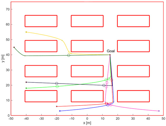
Figure 2.
Starting map for the simulations of the first scenario, including the predefined paths of seven robots. In this scenario, according to their initial trajectories, two robots collide at the coordinates marked by the empty circles. The trajectories for robot 1 to robot 7 are plotted in blue, red, green, black, magenta, yellow and dark green, respectively.
3.1.1. Evaluation Criteria
The primary performance metrics evaluated in this study are the total finish time, the total energy spent and the minimum distance between robots. The total finish time represents the duration required for the last robot to reach the goal, reflecting the efficiency of the system in completing the task. The total energy spent represents the energy consumed by the system of all robots during their trajectories. The minimum distance between robots ensures that the trajectories maintain a safe distance to avoid collisions, validating the effectiveness of the collision avoidance strategy when compared to the safety margin. It is computed as the minimum distance between any pair of robots of the system at each time step of the simulation:
3.1.2. Baseline Methods
The Brute-Force approach provides a baseline for evaluating the effectiveness of the proposed methods. While this method guarantees a collision-free solution, it lacks an optimization process, leading to suboptimal results in both task completion time and computational efficiency. The Prioritized Planning approach significantly improves execution time compared to the Brute-Force method by assigning priorities to robots and sequentially adjusting their velocities to avoid collisions. Since lower-priority robots must adjust their velocities to accommodate higher-priority ones, the method tends to unevenly distribute slow-downs, which can negatively affect overall efficiency.
3.1.3. Maximum Velocity Optimization
To evaluate the Maximum Velocity Optimization approach, multiple simulations were performed. The Genetic Algorithm settings adopted in these simulations are identical across all the optimization approaches proposed in this work, ensuring a fair comparison of results. Elitism was enabled to preserve the best-performing 5% of solutions between generations, while parent selection was carried out using the stochastic uniform selection method to maintain diversity and proportional selection pressure within the population. Key parameters such as CF and MR, defined in Section 2.2, were varied across 9 parameter combinations using Scattered crossover and Uniform mutation [22]. Each combination was executed with a Population Size of 100 individuals for 500 Generations, with 50 independent simulations per configuration.
The results shown in Figure 3 reveal that, for all parameter combinations, the median travel time improves as the MR increases. For the lowest value of CF, it improves from 135 s to 111 s, achieving the best result among all the combinations. For the middle value of CF, it goes from 138 s to 125 s. For the highest value of CF, it drops from 151 s to 132 s.
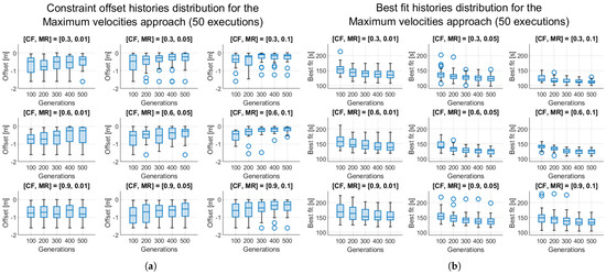
Figure 3.
Box charts of 50 simulations executed with 9 different combinations of Mutation Rate and Crossover Fraction, where every simulation is performed with a population size of 100 individuals: (a) The plots show the distributions of the values of the constraint function every 100 generations, for every simulation. (b) The plots show the distributions of the best fit every 100 generations, for every simulation.
Plots in Figure 3 also show the values of the distributions of the minimum constraint violations, computed as the minimum distance between any two robots in the system, computed as defined in Equation (6), throughout the entire simulation, with the negative sign. These results highlight that higher values of MR generally lead to better optimization outcomes, as they increase the exploration capability of the algorithm, reducing the risk of stagnation in local minima. On the other hand, lower mutation rates restrict the search space, resulting in less optimal solutions. Interestingly, a similar improvement can be observed with lower CF values: when the MR value is fixed, better results are obtained for lower CF values. Indeed, the combination of the lowest CF and the highest MR appears to achieve the best balance between exploration and exploitation, enabling the algorithm to widely explore the solution space.
3.1.4. Slow-Down Segment Approach
This section presents the results of applying the Slow-Down Segment Optimization for the same combinations of MR and CF used in the Maximum Velocity Optimization discussed in the previous section. These simulations also aim to explore the effectiveness of the proposed method under different configurations and provide insights into the optimal parameter settings. First, the effects of the Slow-Down Segment Optimization on the trajectories of the robots are presented. The map shown in Figure 4 illustrates the optimized slow-down segments on the trajectories of the robots. These segments represent the portions of the trajectory where velocity reduction is applied to avoid collisions while optimizing the travel time.
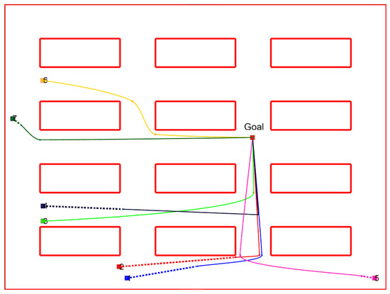
Figure 4.
Map and trajectories modified with the slow-down segment computed through the Slow-Down Segment optimization algorithm. The slow-down segments are plotted as dashed lines. The trajectories for robot 1 to robot 7 are plotted in blue, red, green, black, magenta, yellow and dark green, respectively.
To evaluate the performance of this approach, 50 simulations were conducted across the same 9 combinations of MR and CF as in the previous analysis. Each simulation was executed with a Population Size of 100 and ran for 500 Generations, ensuring consistency in the experimental setup. The results, shown in Figure 5, indicate that the best median travel time of 90 s is achieved with a combination of the highest CF and MR. For the lowest value of CF, the median travel time decreases progressively from 97 s to 93 s, from the lowest to the highest value of MR, respectively. Similarly, for the middle value of CF, the median improves from 94 s to 90 s. For the highest value of CF, the results show remarkable consistency, with median values of 90 s to 90 s. Plots in Figure 5 also show the values of the distributions of the minimum constraint violations.
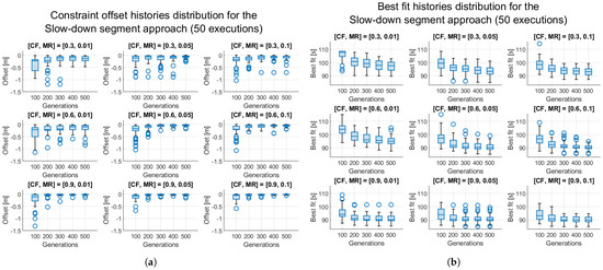
Figure 5.
Box charts of 50 simulations executed with 9 different combinations of Mutation Rate and Crossover Fraction, where every simulation is performed with a population size of 100 individuals: (a) The plots show the distributions of the values of the constraint function every 100 generations, for every simulation. (b) The plots show the distributions of the best fit every 100 generations, for every simulation.
These results demonstrate a significant improvement over the previous Maximum velocity optimization approach, highlighting the effectiveness of the Slow-down Segment strategy. The best median travel time of 90 s achieved represents a substantial reduction compared to the results obtained using the earlier method, where the best overall median was 111 s. Moreover, with this approach, the results improve as the CF increases, unlike in the previous approach.
3.1.5. Multi-Objective Optimization
To evaluate the Multi-Objective Optimization approach, simulations were conducted using the same 9 combinations of MR and CF as in the previous analyses. The results are presented in the form of Pareto fronts in Figure 6, illustrating the trade-off between total travel time and energy consumption. As explained in Section 2.5, these fronts represent the set of non-dominated solutions, where an improvement in one objective (travel time) results in a deterioration of the other (energy consumption). Table 1 lists the best solutions for each of the 9 combinations. The best solution is defined as the Pareto-optimal solution, that is, the closest solution to the origin, in terms of Euclidean distance, among all solutions. Among these, the best Pareto-optimal solution is obtained with the second combination, corresponding to 328 s and 0.26 kJ.
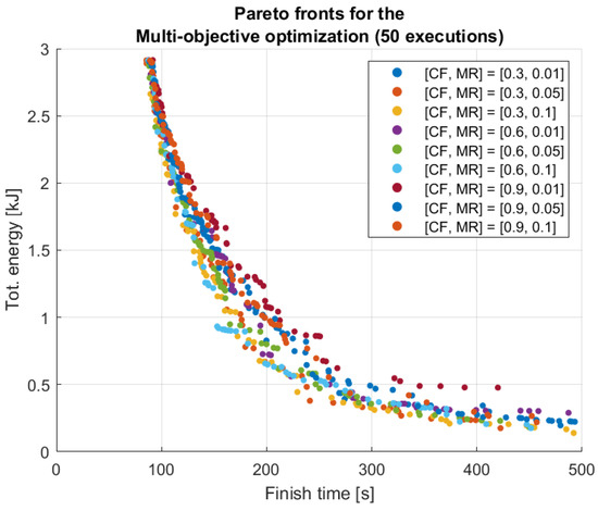
Figure 6.
Plots of the pareto fronts for the Multi-objective optimization for every combination of CF and MR, with a population size of 100 individuals and 500 Generations.

Table 1.
List of Pareto-optimal solutions for every combination of MR and CF, for the simulations presented in Figure 6.
3.2. Second and Third Scenario
To further evaluate the generalization capability of the proposed method, a second and a third simulation scenarios were analyzed, characterized by a larger and more complex environment with irregularly shaped obstacles and narrower passages, as shown in Figure 7. In particular, the map dimensions were increased to 200 × 150 m and 414 × 340 m, respectively, significantly enlarging the operating area compared to the first scenario. The setup again involved seven robots following predefined paths toward a common goal. In these scenarios, the maximum velocity and acceleration were kept at 1.5 m/s and 1 m/s2, respectively. Under these conditions, the system presented 5 collisions and a total finish time of 234 s for the second scenario, and 10 collisions and a total finish time of 686 s for the third scenario. The trajectories shown in Figure 7 correspond to this initial condition, highlighting the collision points before the optimization process. The experiments focused on the Slow-Down Segment Single-Objective Optimization approach, using the parameter combination , which provided the best performance in the previous analysis. The same experimental setup and the parameter settings for the Genetic Algorithm for the previous were maintained. The application of the SDS-SOO optimization successfully resolved all collisions while maintaining efficient task execution. As illustrated in Figure 8, the best median finish time achieved after 500 generations was 255 s for the second scenario and 717 s for the third scenario. The results demonstrate that the framework maintains consistent performance and effective collision avoidance even in more extensive layouts. Compared to the first scenario, the larger map area led to an increased number of trajectory samples for each robot, which in turn resulted in higher computational complexity.
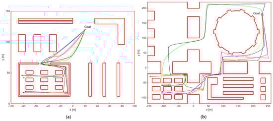
Figure 7.
Starting map for the simulations of the second (a) and the third (b) scenario, including the predefined paths of seven robots. The trajectories for robot 1 to robot 7 are plotted in blue, red, green, black, magenta, yellow and dark green, respectively.
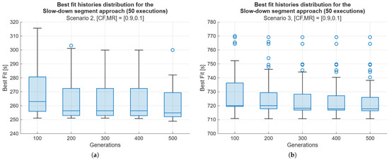
Figure 8.
Box charts of 50 simulations executed with the same combination of Mutation Rate and Crossover Fraction, where every simulation is performed with a population size of 100 individuals. The plots show the distributions of the values of the best fit every 100 generations, for every simulation for the second (a) and the third (b) scenario.
4. Conclusions and Future Developments
The final results for the first scenario, summarized in Table 2, provide a complete comparison between the two baseline methods and the three proposed approaches, respectively: Brute Force (BF), Prioritized Planning (PP), Maximum Velocity Optimization (MVO), Slow-Down Segment Single-Objective Optimization (SDS-SOO), and Slow-Down Segment Multi-Objective Optimization (SDS-MOO). These approaches are evaluated according to the criteria introduced in Section 3.1.1, including finish time, total energy consumption, and execution time.
Table 2.
Comparison of the Evaluation parameters for the results obtained in Section 3.1.3, Section 3.1.4 and Section 3.1.5 for the first scenario.
The values in Table 2 summarize the results obtained in Section 3.1.3, Section 3.1.4 and Section 3.1.5. Only for the SDS-MOO approach, the presented result is the best Pareto-optimal solution across 50 simulations for 9 different combinations of CF and MR, as shown in Section 3.1.5, based on Finish time and Total energy. Mean distance is the mean distance associated with the best Pareto-optimal solution, while Execution time is the best median across all the combinations and simulations.
In the starting scenario, where no collision avoidance strategy is applied, the 7 robots move freely at their maximum allowed velocities, resulting in a finish time of 76 s and a total energy consumption of 3.00 kJ. These values represent the best theoretical performance in terms of travel time but also the worst-case scenario for safety management, since there is still no collision avoidance algorithm involved.
The BF approach, while ensuring a valid collision-free solution, achieves a finish time of 110 s. However, this method lacks optimization, both in terms of execution time and solution quality. With an execution time of 84 min, it is computationally demanding and impractical for real-world applications. In contrast, the PP approach offers an incredibly fast execution time of 0.44 s, but at the cost of the worst finish time of 126 s, underlining the trade-off between computational efficiency and solution quality.
The MVO approach represents the first optimization-based method introduced in this study. It gives a reasonable balance between computational effort and solution quality, achieving a median finish time of 111 s across 50 independent executions and an average execution time of 5 min. This result demonstrates the benefits of introducing optimization techniques into the collision avoidance strategy.
The SDS-SOO approach builds on the strengths of MVO, achieving a median finish time of 90 s. This result marks a substantial improvement over the MVO approach and shows the effectiveness of the Slow-Down Segment Optimization strategy in reducing travel time without increasing computational cost.
Finally, the SDS-MOO approach introduces energy consumption as an additional optimization objective alongside finish time. The best Pareto-optimal solution from the 9 tested parameter combinations achieves a total energy consumption of 0.26 kJ, with a finish time of 328 s. While this specific result does not represent the absolute minimum in travel time or energy, the SDS-MOO approach offers a broader set of Pareto-optimal solutions than the other methods, enabling flexibility based on varying priorities. The SDS-MOO approach clearly performs better in solution diversity and flexibility, offering a rich spectrum of Pareto-optimal solutions. This flexibility enables decision-makers to prioritize either travel time or energy consumption based on specific application requirements, enhancing the adaptability and robustness of the optimization strategy.
The experimental results demonstrated that baseline methods, such as Brute-Force and Prioritized Planning, provide valid but suboptimal solutions. The introduction of optimization-based approaches allowed for a more balanced trade-off between computational efficiency, total travel time, and energy consumption. The Slow-Down Segment Multi-Objective Optimization further improved the framework by introducing Pareto-based optimization, offering decision-makers flexibility in selecting solutions that balance speed and energy efficiency.
To further validate the scalability and robustness of the proposed framework, two additional simulation scenarios were analyzed. These scenarios were characterized by larger and more complex environments, with irregular obstacles and narrower passages. In the initial conditions, 5 and 10 collisions were detected, with total finish times of 234 s and 686 s for the second and third scenarios, respectively. The experiments focused on the SDS-SOO approach, using the parameter combination , which yielded the best performance in the first scenario. The same Genetic Algorithm parameters, namely 100 individuals and 500 generations, were maintained. After the optimization, all collisions were successfully resolved, achieving the best median finish times of 255 s and 717 s. These results confirm that the proposed framework maintains effective collision avoidance and consistent performance even when scaling to larger and more complex environments. The increase in map size led to a higher number of trajectory samples for each robot, resulting in greater computational complexity, yet the optimization process remained stable and efficient. Table 3 summarizes the main quantitative results across the three scenarios. The finish time increase factor, defined as the ratio between the optimized and the initial finish times, progressively decreases from 1.18 in the first scenario to 1.04 in the third, indicating that as the environment grows in size, the relative impact of the collision avoidance task on total travel time becomes smaller. This behavior suggests that the algorithm’s intervention becomes proportionally less invasive in larger layouts, where robots naturally tend to be more spatially distributed. Conversely, the execution time increases approximately linearly with the average path length, which grows from 67 m to 629 m. Although this trend does not represent a rigorous scalability analysis, it provides an initial indication of how computational effort increases with environment size and robot path complexity, setting the basis for future investigations on the framework’s scalability and computational performance. A possible strategy to mitigate execution time growth would be to introduce multi-resolution evaluation techniques, in which the distance computations between robots are initially performed at a lower temporal resolution across the entire population, and progressively refined only for the best-performing individuals. This subsampling approach would allow for a reduction in the number of collision checks in the early stages of the optimization, focusing computational resources on the most promising solutions in later generations, thus preserving accuracy while significantly reducing overall execution time.
Table 3.
Comparison of the results obtained with the Slow-Down Segment—Single-Objective Optimization for the first, second and third scenarios. Finish times are the best median on 50 executions after 500 generations, while execution times are the average of 50 executions.
Future developments will focus on extending the current framework to address more dynamic and uncertain environments, where moving obstacles or unpredictable changes in robot trajectories may occur. This extension will require integrating time-varying constraints and predictive elements into the optimization process, potentially through the inclusion of stochastic optimization techniques. Moreover, additional investigations will compare the performance of the proposed Genetic Algorithm-based approach with other metaheuristic optimization methods, such as Particle Swarm Optimization or Differential Evolution, to assess differences in convergence speed, robustness, and solution quality. Finally, experimental validation will be pursued using a physical multi-robot platform to evaluate the proposed framework under real-world conditions, considering factors such as sensor noise, actuation delays, and communication uncertainties. These advancements will further strengthen the practical applicability of the method and provide a deeper understanding of its performance beyond simulated environments.
Overall, this study highlights the effectiveness of Genetic Algorithm-based optimization for multi-robot coordination, demonstrating its potential for industrial automation, logistics, and autonomous transportation. By addressing these challenges, future research can further refine the approach, improving its adaptability and scalability for real-world applications.
Author Contributions
Conceptualization, L.M. and A.V.; Data curation, L.M.; Methodology, L.M.; Supervision, A.V. and G.D.G.; Validation, L.M.; Writing—original draft, L.M.; Writing—review & editing, A.V. and G.D.G. All authors have read and agreed to the published version of the manuscript.
Funding
This research received no external funding.
Data Availability Statement
The data presented in this study are openly available at https://github.com/marseluca/gapaper (accessed on 30 October 2025).
Acknowledgments
IPFN activities were supported by FCT—Fundação para a Ciência e Tecnologia, I.P. by project reference UIDB/50010/2020 and DOI identifier 10.54499/UIDB/50010/202 (https://doi.org/10.54499/UIDB/50010/2020), by project reference UIDP/50010/2020 and DOI identifier DOI 10.54499/UIDP/50010/2020 (https://doi.org/10.54499/UIDP/50010/2020) and by project reference LA/P/0061/202 and DOI 10.54499/LA/P/0061/2020 (https://doi.org/10.54499/LA/P/0061/2020). This work was also supported by the Erasmus+ program of the European Union and the University of Naples Federico II.
Conflicts of Interest
The authors declare no conflicts of interest.
Abbreviations
The following abbreviations are used in this manuscript:
| GA | Genetic Algorithm |
| MVO | Maximum Velocity Optimization |
| SDS-SOO | Slow-Down Segment–Single-Objective Optimization |
| SDS-MOO | Slow-Down Segment–Multi-Objective Optimization |
| MINLP | Mixed-Integer Non-Linear Programming |
| CF | Crossover Fraction |
| MR | Mutation Rate |
References
- Vale, A.; Ventura, R.; Lopes, P.; Ribeiro, I. Assessment of navigation technologies for automated guided vehicle in nuclear fusion facilities. Robot. Autom. Syst. 2017, 97, 153–170. [Google Scholar] [CrossRef]
- Borenstein, J.; Wehe, D.; Feng, L.; Koren, Y. Mobile robot navigation in narrow aisles with ultrasonic sensors. In Proceedings of the ANS Topical Meeting on Robotics and Remote Systems, Monterey, CA, USA, 5–10 February 1995. [Google Scholar]
- Soh, L.S.; Ho, H.W. Autonomous navigation of micro air vehicles in warehouses using vision-based line following. arXiv 2023, arXiv:2310.00950. [Google Scholar] [CrossRef]
- Poudel, L.; Elagandula, S.; Zhou, W.; Sha, Z. Decentralized and centralized planning for multi-robot additive manufacturing. J. Mech. Des. 2023, 145, 012003. [Google Scholar] [CrossRef]
- Lin, S.; Liu, A.; Wang, J.; Kong, X. A review of path-planning approaches for multiple mobile robots. Machines 2022, 10, 773. [Google Scholar] [CrossRef]
- De Filippo, A.; Lombardi, M.; Milano, M. Off-line and on-line optimization under uncertainty: A case study on energy management. In Proceedings of the Integration of Constraint Programming, Artificial Intelligence, and Operations Research (CPAIOR), Delft, The Netherlands, 26–29 June 2018. [Google Scholar]
- Van Den Berg, J.; Snoeyink, J.; Lin, M.; Manocha, D. Centralized path planning for multiple robots: Optimal decoupling into sequential plans. In Proceedings of the Robotics: Science and Systems (RSS), Seattle, WA, USA, 28 June–1 July 2009. [Google Scholar]
- Luna, R.; Bekris, K. Efficient and complete centralized multi-robot path planning. In Proceedings of the IEEE/RSJ International Conference on Intelligent Robots and Systems (IROS), San Francisco, CA, USA, 25–30 September 2011. [Google Scholar]
- Jose, K.; Pratihar, D.K. Task allocation and collision-free path planning of centralized multi-robots system for industrial plant inspection using heuristic methods. Robot. Auton. Syst. 2016, 80, 34–42. [Google Scholar] [CrossRef]
- Jose, K.; Pratihar, D.K. Efficient multi-robot path planning in real environments: A centralized coordination system. Int. J. Intell. Robot. Appl. 2024, 9, 217–244. [Google Scholar] [CrossRef]
- Zhu, H.; Brito, B.; Alonso-Mora, J. Decentralized probabilistic multi-robot collision avoidance using buffered uncertainty-aware Voronoi cells. Auton. Robot. 2022, 46, 401–420. [Google Scholar] [CrossRef]
- Long, P.; Fan, T.; Liao, X.; Liu, W.; Zhang, H.; Pan, J. Towards optimally decentralized multi-robot collision avoidance via deep reinforcement learning. In Proceedings of the IEEE International Conference on Robotics and Automation (ICRA), Brisbane, QLD, Australia, 21–25 May 2018; pp. 6252–6259. [Google Scholar]
- Sano, Y.; Endo, T.; Shibuya, T.; Matsuno, F. Decentralized navigation and collision avoidance for robotic swarm with heterogeneous abilities. Adv. Robot. 2022, 37, 25–36. [Google Scholar] [CrossRef]
- Ferrera, E.; Castano, A.; Capitàn, J.; Ollero, A.; Marròn, P. Decentralized collision avoidance for large teams of robots. In Proceedings of the 16th International Conference on Advanced Robotics (ICAR), Montevideo, Uruguay, 25–29 November 2013. [Google Scholar]
- Van Den Berg, J.; Lin, M.; Manocha, D. Reciprocal velocity obstacles for real-time multi-agent navigation. In Proceedings of the IEEE International Conference on Robotics and Automation (ICRA), Pasadena, CA, USA, 19–23 May 2008. [Google Scholar]
- Wilkie, D.; Van Den Berg, J.; Manocha, D. Generalized velocity obstacles. In Proceedings of the IEEE/RSJ International Conference on Intelligent Robots and Systems (IROS), St. Louis, MO, USA, 10–15 October 2009. [Google Scholar]
- Rabbouch, B.; Rabbouch, H.; Saadaoui, F.; Mraihi, R. Foundations of combinatorial optimization, heuristics, and metaheuristics. In Comprehensive Metaheuristics: Algorithms and Applications; Elsevier: Amsterdam, The Netherlands, 2023. [Google Scholar]
- Belotti, P.; Kirches, C.; Leyffer, S.; Linderoth, J.; Luedtke, J.; Mahajan, A. Mixed-integer nonlinear optimization. Acta Numer. 2013, 22, 1–131. [Google Scholar] [CrossRef]
- Floudas, C.A. Nonlinear and Mixed-Integer Optimization: Fundamentals and Applications; Oxford University Press: Oxford, UK, 1995. [Google Scholar]
- Alam, T.; Qamar, S.; Dixit, A.; Benaida, M. Genetic algorithm: Reviews, implementations, and applications. Int. J. Eng. Pedagog. (IJEP) 2020, 10, 57–77. [Google Scholar] [CrossRef]
- Deep, K.; Kansal, M.L.; Singh, K.P.; Mohan, C. A real coded genetic algorithm for solving integer and mixed integer optimization problems. Appl. Math. Comput. 2009, 212, 505–518. [Google Scholar] [CrossRef]
- Eiben, A.; Smith, J. Introduction to Evolutionary Computing; Springer: Berlin/Heidelberg, Germany, 2003. [Google Scholar]
- Moehle, N. Optimal racing of an energy-limited vehicle. Harv. Tech. Rep. 2013. [Google Scholar] [CrossRef]
- Bre, F.; Fachinotti, V. A computational multi-objective optimization method to improve energy efficiency and thermal comfort in dwellings. Energy Build. 2017, 154, 283–294. [Google Scholar] [CrossRef]
- Van Den Berg, J. Prioritized motion planning for multiple robots. In Proceedings of the IEEE/RSJ International Conference on Intelligent Robots and Systems (IROS), Edmonton, AB, Canada, 2–6 August 2005. [Google Scholar]


Disclaimer/Publisher’s Note: The statements, opinions and data contained in all publications are solely those of the individual author(s) and contributor(s) and not of MDPI and/or the editor(s). MDPI and/or the editor(s) disclaim responsibility for any injury to people or property resulting from any ideas, methods, instructions or products referred to in the content. |
© 2025 by the authors. Licensee MDPI, Basel, Switzerland. This article is an open access article distributed under the terms and conditions of the Creative Commons Attribution (CC BY) license (https://creativecommons.org/licenses/by/4.0/).