Cutting Tool Remaining Useful Life Prediction Using Multi-Sensor Data Fusion Through Graph Neural Networks and Transformers

Abstract

In the context of Industry 4.0 and smart manufacturing, predicting cutting tool remaining useful life (RUL) is crucial for enabling and enhancing the reliability and efficiency of CNC machining. This paper presents an innovative predictive model based on the data fusion architecture of Graph Neural Networks (GNNs) and Transformers to address the complexity of shallow multimodal data fusion, insufficient relational modeling, and single-task limitations simultaneously. The model harnesses time-series data, geometric information, operational parameters, and phase contexts through dedicated encoders, employs graph attention networks (GATs) to infer complex structural dependencies, and utilizes a cross-modal Transformer decoder to generate fused features. A dual-head output enables collaborative RUL regression and health state classification of cutting tools. Experiments are conducted on a multimodal dataset of 824 entries derived from multi-sensor data, constructing a systematic framework centered on tool flank wear width (VB), which includes correlation analysis, trend modeling, and risk assessment. Results demonstrate that the proposed model outperforms baseline models, with MSE reduced by 26–41%, MAE by 33–43%, R² improved by 6–12%, accuracy by 6–12%, and F1-Score by 7–14%.

1. Introduction

In sustainable manufacturing and Industry 4.0, digitization, cloud computing, and intelligent systems drive innovations by enhancing precision and sustainability. Numerical control (CNC) machine tools, as foundational “mother machines” for high-value manufacturing, underpin modern industry through their automation, precision, and reliability, profoundly impacting efficiency and quality in sectors like aerospace, automotive, and precision engineering [1]. Cutting tools, the critical end-effectors in CNC systems, interact directly with workpieces but are highly vulnerable to failure under harsh conditions involving mechanical impacts, high temperatures, pressures, and friction, leading to wear, damage, or chipping.

In harsh cutting environments, cutting tools continuously endure intense mechanical impacts, high temperatures and pressures, as well as severe friction, making forms of failure such as wear, damage, or even chipping inevitable. Progressive tool failure not only directly leads to a decline in workpiece surface quality, dimensional inaccuracies, and increased scrap rates; more severely, sudden tool breakage can cause catastrophic secondary damage, such as harming the workpiece, fixtures, or even core expensive components like the machine spindle, resulting in significant economic losses and production safety accidents [2]. Traditional manufacturing employs experience-based periodic tool changes to mitigate risks, but this passive approach overlooks tool life variability from diverse conditions and materials, leading to premature discard of tools with substantial RUL and resource waste, contradicting green manufacturing principles [3]. Intelligent technologies for real-time tool health assessment and RUL prediction are essential to transition from “time-based” passive to “condition-based” predictive maintenance, a key focus in academia and industry [4]. Accurate RUL prediction prevents failures, ensures safety, optimizes efficiency, maximizes tool utilization, integrates tool changes into scheduling to minimize downtime, and supports intelligent, unmanned factories like “lights-out” operations, bridging sensing and decision-making.

However, despite significant progress in data-driven prediction methods in recent years [5,6], their applications to complex and variable real-world industrial scenarios still face a series of deep-seated challenges, which constitute the current technical bottlenecks in research. First, existing methods show deficiencies in multimodal data fusion, often using simple concatenation or weighting that ignores deep nonlinear interactions among time-series signals for cutting dynamics, geometric information for wear states, and static parameters for operating conditions [7]. Second, they fail to exploit structural dependencies, as traditional models handle Euclidean data well but overlook non-Euclidean graph structures in machining. For instance, entities include tools as nodes representing wear states, sensors capturing force and roughness signals, workpieces linked to surface quality metrics, and experimental phases grouping sequential operations. Relationships manifest as edges denoting dependencies, such as the physical coupling between tool wear VB in mm and cutting forces Fx/Fy/Fz from sensors, or contextual links across batches that reflect variability in machining conditions and degradation patterns. Ignoring these graphs limits generalization and robustness [8]. Finally, single-task regression overlooks health state transitions, such as from “normal” to “rapid wear”, failing to provide staged maintenance guidance. This paper addresses these challenges by integrating GNNs with optimized Transformers for deep multimodal fusion, precise graph relational inference, and multi-task learning, enabling simultaneous RUL prediction and health state classification in dynamic machining processes.

2. Literature Review

Cutting tool RUL prediction is a core topic in the field of smart manufacturing. Domestic and international research revolves around three technical routes: physical and statistical models, traditional machine learning and ensemble learning, and deep learning. These routes have, respectively, advanced prediction accuracy and generalization capabilities in theoretical depth, algorithm optimization, and industrial applications.

Physical and statistical models use mathematical equations for mechanistic and data-driven predictions. Physical modeling, constrained by multivariable complexity, guides data methods via fusion; for example, physics-informed hidden Markov model (PI-HMM) [9] and Gaussian process regression [10] improve consistency and uncertainty, while early HMMs tracked wear using forces [11]. Statistical approaches like multi-stage Wiener processes with change-point detection characterize non-stationary wear phases [12,13].

Traditional machine learning and ensemble learning build efficient models from sensor data, emphasizing accuracy and uncertainty. Support Vector Machines (SVMs) hybrids incorporate particle filtering or optimization for time-series and limited-data scenarios [14,15]; Gaussian Process Regression (GPR) variants handle noise via sparsity or genetic algorithms [16,17]. Bayesian methods prevent overfitting and quantify uncertainty [18], with early inference networks [19] and recent Bayesian Regularized Artificial Neural Networks (BRANNs) [20] enabling robust generalization. Ensembles, including random forests [21,22] and Extreme Gradient Boosting (XGBoost) hybrids [23,24], excel in classification and optimization, while AdaBoost suits small datasets [25]; comparative studies highlight reliable selection for reliability prediction [26].

Deep learning enables end-to-end feature learning for robust architectures. Automated analysis employs Fully Convolutional Networks (FCNs) [27] or lightweight Convolutional Neural Networks (CNNs) [28] for high-accuracy wear detection. In aerospace, autoencoders with Gated Recurrent Units (GRUs) monitor composites [29]. Recurrent models like adaptive Bidirectional Long Short-Term Memory networks (BiLSTMs) [30,31] and multi-sensor Long Short-Term Memory networks (LSTMs) [32] capture dependencies. Hybrids fuse features via wavelets [33] or attention with Independently Recurrent Neural Network (IndRNN) [34]; multirate Hidden Markov Models (HMMs) process acoustics [35], and Maximal Overlap Discrete Wavelet Transform (MODWT) supports label-free IoT predictions [36]. Time–frequency LSTMs [37] and Transformers like Power Spectral Density–Convolutional Vision Transformer (PSD-CVT) [38] or Convolutional Physics-Informed Transformer (Conv-PhyFormer) [39] balance efficiency and interpretability. Physics-informed Deep Learning (DL) optimizes generalization [40].

Although these studies have advanced tool RUL prediction from mechanism-driven to data-driven paradigms, three core challenges remain: shallow multimodal fusion overlooking physical couplings and contexts, for example, batches and sequences, leading to biases and reduced robustness under noise; inadequate relational modeling of non-Euclidean graphs among entities like tools and sensors, causing redundancy and weakened generalization in variable scenarios; and single-task regression neglecting health state evolution, limiting staged degradation sensitivity and maintenance guidance.

To overcome these, this study proposes an innovative end-to-end architecture integrating multimodal encoding, graph relational inference, and multi-task learning for deep fusion and interaction. Modal encoders refine feature extraction, preserving modality traits with adaptive weighting to address imbalances and exceed concatenation limits. A graph adaptive fusion module uses GATs to construct and learn entity dependency graphs, dynamically attending to nonlinear interactions and contextual links for enhanced robustness in noisy environments. Finally, a cross-modal Transformer decoder fuses global features via self-attention across time-series, geometric, and operational data, enabling dual-head multi-task outputs, one for health state classification and one for RUL regression, to promote knowledge transfer, degradation sensitivity, and precise predictions.

3. Architecture Design for Tool RUL Calculation

The architecture design encompasses key stages such as data acquisition, feature engineering, multimodal feature extraction, graph adaptive fusion, and cross-modal interaction and prediction, aiming to achieve high-precision RUL regression prediction and health status classification of the cutting tool.

Figure 1 completely depicts a multimodal deep learning model for precisely predicting the tool RUL and assessing its health status. The core idea of this model is to systematically integrate data from different information sources to build a comprehensive understanding of the tool wear process. The entire process begins with data acquisition phase, which acquires four key types of data in parallel: first, raw sensor data that directly reflects the physical state of the cutting process, such as three-directional cutting forces (Fx, Fy, Fz) and a series of surface roughness parameters; second, geometric data that quantify the physical wear of the cutting tool, namely the diameter changes before and after tool use; furthermore, operational parameters that define the machining conditions, including cutting depth, speed, and feed rate; finally, phase information that provides context for the data, such as experimental batches and positions. These four types of data together lay a solid data foundation for the subsequent precise predictions, particularly in the semantics of cutting force variations, tool cutting edge status, tool wear, surface roughness and quality of the component machined [41].

After data acquisition, the system enters the feature engineering and preprocessing stage, with the objective of transforming raw data into more informative features to prepare for the deep learning model. In this stage, high-frequency sensor signals undergo processing through specialized high-order feature extraction algorithms to reveal their intrinsic patterns. The initial and final diameters of the tool are used to calculate a key wear indicator that is VB, which intuitively reflects the degree of tool degradation. At the same time, operational parameters and experimental phase information are, respectively, integrated and embedded encoded, enabling effective mathematical fusion with other types of features.

Next, the architecture employs a parallel multimodal feature processing pipeline to perform deep feature extraction on different data sources. For the cutting force signals that best reflect the real-time cutting state, the system uses a one-dimensional convolutional neural network (1D-CNN) with three convolutional layers, kernel size of 5, and filter dimensions of [64, 128, 256] for envelope extraction, followed by a bidirectional Transformer encoder configured with four layers, eight attention heads, a hidden dimension of 256, and a dropout rate of 0.1 to capture its complex temporal dependencies. For the geometric and roughness data that represent progressive wear, it is processed through a channel that combines a Temporal Convolutional Network (TCN) with four layers, kernel size of 3, channel dimensions of [32, 64, 128, 256], and a standard Transformer encoder with three layers, four attention heads, a hidden dimension of 128, and a dropout rate of 0.1. At the same time, the processed operational parameters and phase information are also forwarded as independent feature streams. This specialized processing ensures that the unique characteristics of each data modality are fully exploited.

One of the innovative aspects of this architecture is its graph adaptive fusion module, which aims to intelligently integrate information from different data streams. This module constructs the features from the geometric, operational parameters, and phase information streams into a graph structure, where the graph’s nodes represent sensor positions, and the edges cleverly define the complex associations between internal tool features as well as between different machining batches. To provide a precise definition, the graph is formulated as G consisting of nodes V and edges E. The nodes V consist of multimodal entities: sensor nodes representing positions for cutting force signals Fx, Fy, Fz and roughness parameters Ra, Rz, embedded as feature vectors from their respective encoders; geometric nodes capturing tool wear metrics like VB and diameter changes; operational parameter nodes encoding static conditions such as cutting depth, speed, and feed rate via dense embeddings; and phase nodes representing experimental batches and positions as categorical embeddings to provide contextual grouping. This integration relates sensor positions to operational and phase info by treating them as interconnected entities in a heterogeneous graph, where sensor nodes are linked to phase nodes for batch-specific context and to operational nodes for condition-dependent dynamics. The edges E are defined based on domain-informed associations: intra-modal edges connect similar entities within a modality, sensor nodes linked by spatial proximity or signal correlation, weighted by cosine similarity of their feature vectors; inter-modal edges capture cross-dependencies such as between geometric nodes VB and sensor nodes forces to model physical coupling, initially weighted by correlation coefficients, strong edge for VB-Fx with correlation >0.7, or between phase nodes and all others to encode batch-wise temporal relations, weighted by sequence similarity across machining cycles. Edges are undirected and initially static but dynamically refined via the attention mechanism of GATs during training, allowing adaptive weighting based on learned importance. By employing GATs with three layers, eight attention heads, a hidden dimension of 256, output dimension of 128, dropout rate of 0.2, and LeakyReLU negative slope (alpha) of 0.2, the model can adaptively learn the importance of different information sources and generate a highly condensed feature representation that is aligned across modalities and batches, providing key context for understanding the tool’s wear behavior under different operating conditions and time scales.

In the final cross-modal interaction and prediction stage, all refined feature information is aggregated to generate the final prediction results. The deep temporal features extracted from the cutting force signals, along with the aligned contextual features output from the graph fusion module, are fed together into a cross-modal Transformer decoder configured with two layers, eight attention heads, a hidden dimension of 256, feed-forward network dimension of 512, and dropout rate of 0.1. This decoder is responsible for parsing and fusing the deep interactions between these two major categories of heterogeneous features, generating the final fused contextual features. These features contain the most comprehensive description of the tool’s current state and are fed into a dual-task output layer. Among them, a classification head consisting of fully connected layers with dimensions [256, 128, 3], ReLU activation, and Softmax function, through fully connected layers and a Softmax function, determines whether the tool is in a “normal,” “warning,” or “critical” health status. Meanwhile, another regression head that is RUL regression head composed of fully connected layers with dimensions [256, 128, 64, 1], ReLU activation, and Sigmoid output solves a key regression problem through a set of fully connected layers: predicting the normalized proportion of the tool’s RUL. To enhance the model’s generalization ability and training stability, the RUL here is normalized to a standard interval of 0 to 1. In this interval, “1” represents the tool in a brand-new state, possessing its full potential useful life; while “0” represents that the tool’s life has been completely exhausted, reaching the failure standard. Therefore, the task of this regression head is to precisely predict a continuous value between 0 and 1, which intuitively represents the percentage of the tool’s current remaining life in its total life. This normalized prediction value not only facilitates robust regression calculations for the model but also provides a standardized health metric independent of specific physical units. When needing to obtain specific physical life, simply multiply this prediction proportion by the total design life of that model tool under specific operating conditions to easily convert to actual remaining minutes or the number of machinable workpieces.

The model training process employs the AdamW optimizer with a learning rate of 1 × 10⁻⁴, incorporating a warmup phase of 500 steps followed by cosine annealing decay. Training is conducted with a batch size of 32 for 100 epochs, with early stopping implemented using a patience of 15 epochs to prevent overfitting. The dual-task joint loss function balances the classification and regression objectives with a lambda (λ) value of 0.7, meaning the regression task contributes 70% to the total loss while the classification task contributes 30%. Specifically, the classification task employs cross-entropy loss with label smoothing of 0.1, and the regression task uses mean squared error (MSE) loss. To stabilize training, gradient clipping with a maximum norm of 1.0 is applied. All experiments are conducted using PyTorch framework (https://pytorch.org/) on an NVIDIA RTX 3090 GPU with 24 GB memory (NVIDIA, Santa Clara, CA, USA).

Based on the macroscopic overview of the tool RUL calculation architecture, this study systematically elaborates the end-to-end process of the model from data acquisition to prediction output. To advance theoretical exploration, the following will delve into the mathematical modeling of each module, as well as the loss functions and optimization strategies. Equations are as (1) to (5). The aim is to provide a quantitative framework for the internal mechanisms of the model, while explaining the theoretical basis for design decisions.

①

VB Mathematical Modeling

$$VB\approx {\displaystyle \frac{D_{\mathrm{i}\mathrm{n}\mathrm{i}\mathrm{t}}-D_{\mathrm{f}\mathrm{i}\mathrm{n}\mathrm{a}\mathrm{l}}}{2}}$$

(1)

where $D_{\mathrm{i}\mathrm{n}\mathrm{i}\mathrm{t}}$ ($\mathrm{I}\mathrm{n}\mathrm{i}\mathrm{t}\_\mathrm{d}\mathrm{i}\mathrm{a}\mathrm{m}\mathrm{e}\mathrm{t}\mathrm{e}\mathrm{r}$) represents the initial diameter of the tool, $D_{\mathrm{f}\mathrm{i}\mathrm{n}\mathrm{a}\mathrm{l}}$ ($\mathrm{F}\mathrm{i}\mathrm{n}\mathrm{a}\mathrm{l}\_\mathrm{d}\mathrm{i}\mathrm{a}\mathrm{m}\mathrm{e}\mathrm{t}\mathrm{e}\mathrm{r}$) represents the current measured diameter. To clarify, VB is a calculated metric derived from direct measurements of the tool’s initial and current diameters. $D_{\mathrm{i}\mathrm{n}\mathrm{i}\mathrm{t}}$ is measured before tool usage, $D_{\mathrm{f}\mathrm{i}\mathrm{n}\mathrm{a}\mathrm{l}}$ is similarly measured after a period of machining, reflecting the tool’s worn state. VB is then computed as the difference between these two measured values. The role of VB is to transform static geometric data into dynamic wear indicators, facilitating fusion with temporal sensor signals.

②

RUL Normalization

$${RUL}_{\mathrm{normalized}}={\displaystyle \frac{L_{\mathrm{r}\mathrm{e}\mathrm{m}\mathrm{a}\mathrm{i}\mathrm{n}\mathrm{i}\mathrm{n}\mathrm{g}}}{L_{\mathrm{t}\mathrm{o}\mathrm{t}\mathrm{a}\mathrm{l}}}}$$

(2)

where $L_{\mathrm{r}\mathrm{e}\mathrm{m}\mathrm{a}\mathrm{i}\mathrm{n}\mathrm{i}\mathrm{n}\mathrm{g}}$ is the current RUL, and $L_{\mathrm{t}\mathrm{o}\mathrm{t}\mathrm{a}\mathrm{l}}$ is the total design life of the tool under specific operating conditions. The [0, 1] interval facilitates sigmoid activation, MSE stability, and cross-unit generalization.

③

ATs Attention Mechanism

The attention coefficient ${\alpha }_{ij}$ for node $i$ aggregating information from neighbor $j$ is computed as follows:

$${\alpha }_{ij}={\displaystyle \frac{\mathrm{e}\mathrm{x}\mathrm{p}\left(\mathrm{L}\mathrm{e}\mathrm{a}\mathrm{k}\mathrm{y}\mathrm{R}\mathrm{e}\mathrm{L}\mathrm{U}\left({\mathrm{a}}^{\mathrm{T}}\left[{\mathrm{W}\mathrm{h}}_i\parallel {\mathrm{W}\mathrm{h}}_j\right]\right)\right)}{\sum _{k\in \mathcal{N}\left(i\right)}\mathrm{e}\mathrm{x}\mathrm{p}\left(\mathrm{L}\mathrm{e}\mathrm{a}\mathrm{k}\mathrm{y}\mathrm{R}\mathrm{e}\mathrm{L}\mathrm{U}\left({\mathrm{a}}^{\mathrm{T}}\left[{\mathrm{W}\mathrm{h}}_{\mathrm{i}}\parallel {\mathrm{W}\mathrm{h}}_{\mathrm{k}}\right]\right)\right)}}$$

(3)

where ${\mathrm{h}}_i$, ${\mathrm{h}}_j$, and ${\mathrm{h}}_k$ are node vectors, representing the embedded feature representations of nodes in the graph G consisting of V and E, where ${\mathrm{h}}_i$ is the central node such as a sensor node encoding cutting force features, ${\mathrm{h}}_j$ and ${\mathrm{h}}_k$ are neighboring nodes such as geometric nodes for VB or operational parameter nodes for cutting conditions, transformed by the weight matrix W to project them into a common space for attention computation, $\mathrm{W}$ is the learnable weight matrix, $\mathrm{a}$ is the attention vector, $i$ represents vector concatenation, $\parallel$ represents vector concatenation, $\mathcal{N}\left(i\right)$ is the set of neighboring nodes of $i$ including $i$ itself for self-attention if applicable, and $\mathrm{L}\mathrm{e}\mathrm{a}\mathrm{k}\mathrm{y}\mathrm{R}\mathrm{e}\mathrm{L}\mathrm{U}$ introduces nonlinearity. This softmax mechanism dynamically weights the edges, enhancing cross-modal robustness.

④

1D-CNN Convolution Operation

$$y_t={\sum }_{k=0}^{K-1}{x}_{t-k}\cdot w_k+b$$

(4)

where $y_t$ is the output feature value at position or time step $t$, representing the convolved result that captures local patterns in the sequence, $\sum _{k=0}^{K-1}$ denotes the summation over the kernel range from $K$ = $0$ to $K$ − $1$, aggregating weighted inputs for efficient feature computation, $x_{t-k}$ is the input signal value at the shifted position $t-k$, providing the sliding window of sequential data such as sensor readings, $w_k$ is the kernel weight at position $k$, and $b$ is the bias term.

⑤

Dual-Task Joint Loss

$$L_{\mathrm{t}\mathrm{o}\mathrm{t}\mathrm{a}\mathrm{l}}=\lambda \cdot L_{\mathrm{regression}}+\left(1-\lambda \right)\cdot L_{\mathrm{classification}}$$

(5)

where $L_{\mathrm{t}\mathrm{o}\mathrm{t}\mathrm{a}\mathrm{l}}$ is the total combined loss function for the multi-task learning model, serving as the overall objective to minimize during training by balancing regression and classification tasks, $\lambda$ is the hyperparameter that controls the relative importance of the regression task, with higher values prioritizing regression over classification (set to 0.7 in our implementation), $L_{\mathrm{regression}}$ is the loss value for the regression task (computed using mean squared error), and $L_{\mathrm{classification}}$ is the loss value for the classification task (computed using cross-entropy loss).

This architecture design drives multimodal fusion with VB as the core degradation indicator. In the feature engineering stage, VB serves as a key proxy, supporting static correlation analysis and segmented trend modeling. The model captures the weak correlations between VB and cutting forces, roughness, and in the graph adaptive fusion module, adaptively weights through the GATs attention mechanism, for risk interval division and multimodal dimensionality reduction.

4. Experiments and Simulations Development

4.1. Dataset

This dataset contains 824 tool observation records with multimodal data from force sensors, surface roughness measurement instruments, and tool monitoring systems, fully reproducing the degradation trajectory of the tool from initial run-in to stable cutting [42]. The dataset is structured into three subsets corresponding to different experimental phases: Prep (run-in period), Experiment 1, and Experiment 2 (stable cutting periods). It encompasses data from 13 distinct cutting tools, and each cutting tool has a total of more than 60 observations across various stages and repeated measurements. The total 824 entries are distributed as follows: Prep stage with 212 entries including initial measurements for all tools, Experiment 1 with 324 samples under new-tool conditions, and Experiment 2 with 288 additional samples under progressive wear conditions, allowing for comprehensive tracking of tool degradation over time. The Prep stage records geometric diameters, cumulative machining time (CTime), machined length, and six surface roughness indicators (Ra, Rz, Rsk, Rku, RSm, Rt), used to identify run-in period features; the stable cutting stage adds three-axis cutting forces (Fx, Fy, Fz) and resultant force F, combined with geometric wear and surface quality data, supporting multimodal analysis. To facilitate model training and evaluation, the dataset was split into training, validation, and testing sets using a stratified approach to preserve the distribution of tool wear levels (VB values) and experimental phases: 70% (578 records) for training, 15% (123 records) for validation, and 15% (123 records) for an independent testing set.

4.2. Experiments and Simulations

Based on the three datasets of Prep, Experiment 1, and Experiment 2, as well as the core parameter VB therein, this article constructs a systematic and hierarchical experimental research framework around the VB-driven RUL prediction task. This framework covers six dimensions: static correlation analysis, temporal trend modeling, risk interval division, multimodal interpretation and dimensionality reduction, uncertainty propagation assessment, and prediction performance and failure determination.

The design of the six dimensions in this experimental research framework follows a progressive closed-loop logic from data exploration to model validation, and then to application optimization: first, static correlation analysis lays the foundation for variable relationships, identifying the core driving role of VB; second, temporal trend modeling captures the dynamic degradation process, bridging from static to dynamic evolution; then, risk interval division introduces application-oriented risk management, quantifying failure warnings; next, multimodal interpretation and dimensionality reduction refine high-dimensional semantics, supporting feature optimization; subsequently, uncertainty propagation assessment diagnoses model reliability, ensuring robustness; finally, prediction performance and failure determination close the evaluation loop, verifying the overall efficacy of GNNs and Transformers.

4.2.1. Static Correlation Analysis

We aimed to explore the relationships between VB and other variables, including surface roughness, cutting forces, and time, through static correlation visualizations. Specifically, tools such as residual analysis plots, scatter plots, and heatmaps were employed to quantify the negative correlation between VB and RUL, the proxy relationship between VB and cutting force components, and the representational value of VB in the surface quality dimension. These associations directly guide the graph construction of GNNs and the feature selection for Transformers.

First, the scatter plot and residual analysis plot of VB and RUL, as shown in Figure 2, demonstrate a strong negative correlation between VB and RUL, thereby verifying the rationality of VB as the main degradation driving variable. The residual analysis plot shows that the error points are basically randomly distributed around the zero line (red dashed line), though the smoothed trend line (orange) reveals a noticeable dip and subsequent rise, particularly between predicted RUL values of 0.4 and 0.5, suggesting a potential systematic bias in this mid-range region where the model may slightly overestimate or underestimate residuals during moderate wear stages. Additionally, the variance of residuals appears to decrease as predicted RUL increases, indicating possible heteroscedasticity rather than perfect homoscedasticity, which could imply that the model’s error distribution is not entirely constant across wear levels and may be influenced by data density in high-RUL (low-wear) areas. Despite these observations, the overall proximity of the trend line to horizontal and the general random scatter support a low level of systematic bias, affirming the model’s reasonable reliability for RUL prediction based on VB. The color gradient (from purple to yellow) encodes the VB values, revealing the relative independence of the residual distribution from the degree of wear. This critical analysis of the residuals highlights areas for refinement, such as incorporating additional data in mid-wear regimes to mitigate bias, while still confirming VB’s utility in guiding GNN graph representations for degradation modeling.

Secondly, the comparative scatter plots of VB and cutting force components (Fx, Fy, Fz) as well as the prediction performance analysis, as shown in Figure 3, explore the systematic patterns of VB with increasing force values, to verify the feasibility of cutting force signals as proxy indicators for VB. Fx shows the strongest positive correlation, with a larger regression line slope; Fy lacks correlation, with a horizontal trend line; Fz shows moderate positive correlation, with a medium and positive regression line slope, but high dispersion. The prediction accuracy scatter plot shows values closely along the perfect line; the residual distribution is random and unbiased; the error histogram approximates normal; the feature importance bar chart confirms Fx as dominant, Fz second, and Fy lowest. These results guide GNNs node aggregation, prioritizing Fx, and enhance model interpretability.

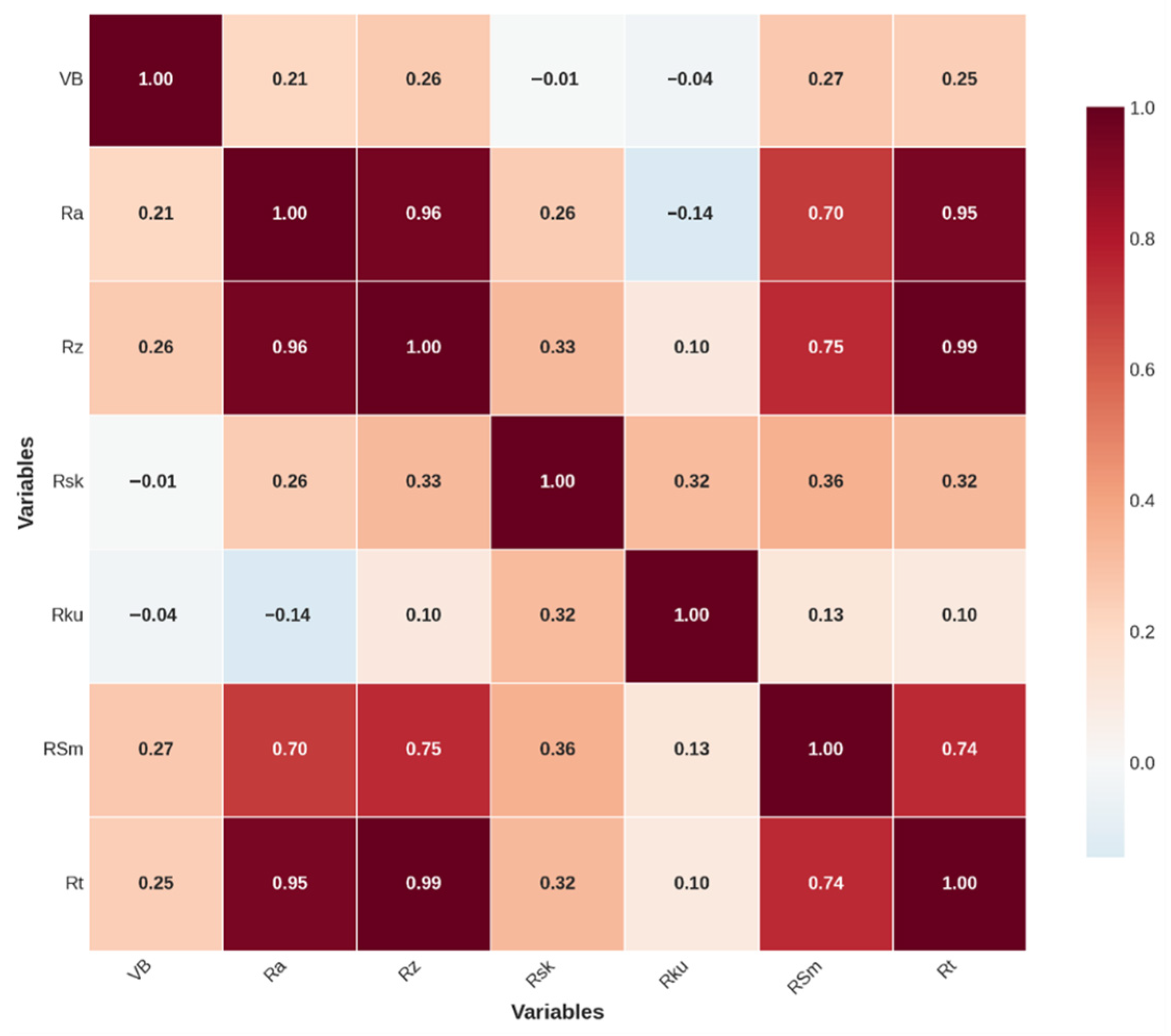
Finally, the VB and roughness multivariable correlation heatmap, as shown in Figure 4, calculate the correlation coefficients between VB and Ra, Rz, Rsk, Rku, RSm, and Rt to assess the representational value of VB in the surface quality dimension. The heatmap shows weak positive correlations between VB and RSm, Rz, and Rt, with no correlation to Rsk and Rku; the roughness parameters are highly correlated internally. The weak positive correlations indicate the need for Transformer multimodal fusion to enhance the assessment.

4.2.2. Temporal Trend Modeling

Based on key variables identified through static correlation, the dynamic trends of VB are revealed through time-series visualization, comparing the evolution patterns of tool wear. These identify nonlinear changes, supporting Transformer sequence modeling and GNNs’ dynamic graph updates. Time-series trends can serve as input sequences for the GNNs-Transformer, verifying its superiority in capturing phase transitions.

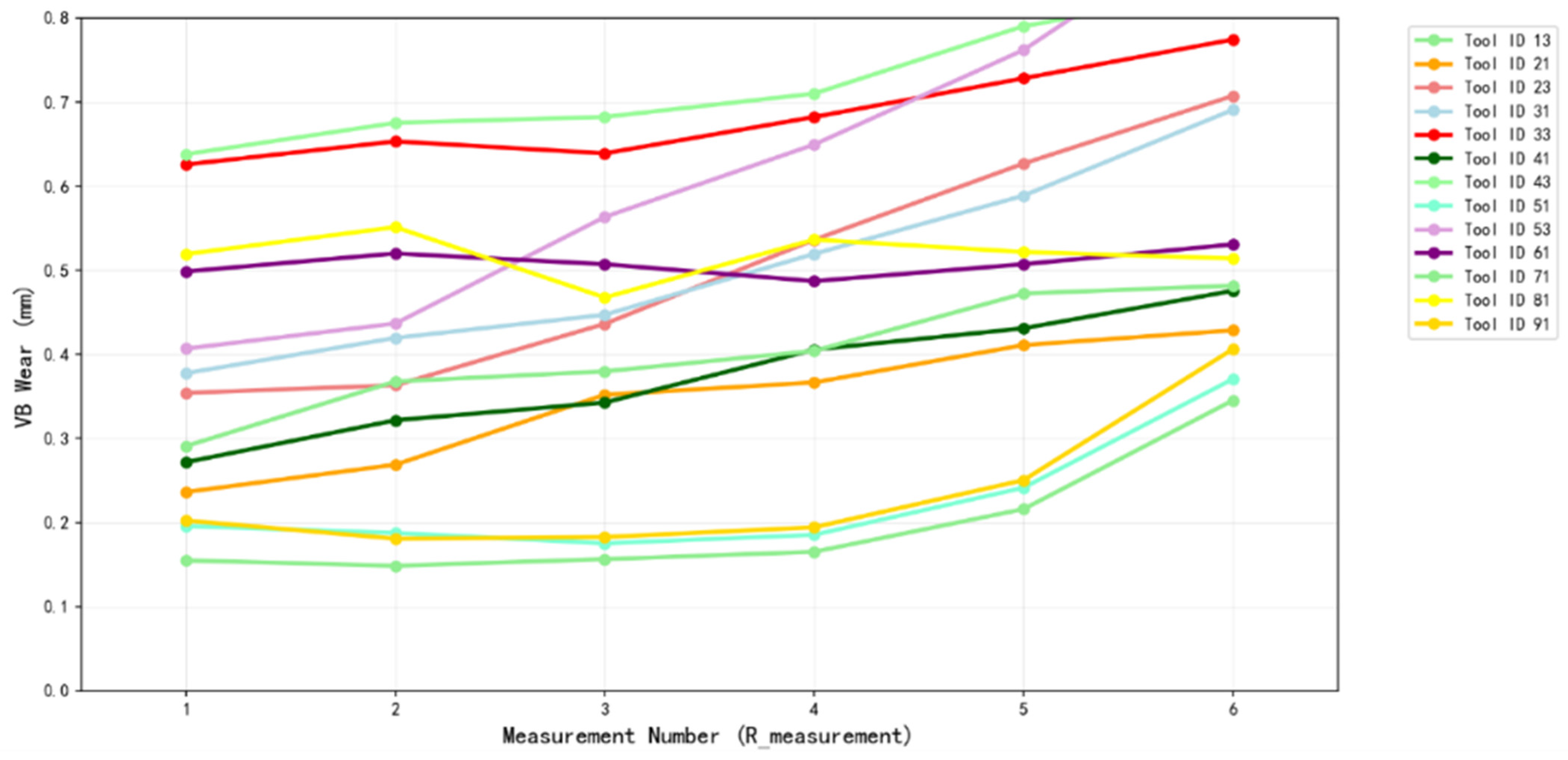
Firstly, the degradation trajectory plot and nonlinear curve plot of VB changing with the measurement number (R_measurement), as shown in Figure 5, plots multiple VB curves according to Tool_ID, comparing the wear progress trajectories of different tools. The results show that the 13 tools overall exhibit a progressive increasing pattern, starting from initial low values, rising slowly or at medium speed with the number of measurements, and reaching varying levels of 0.3–0.8 mm by the sixth measurement.

Secondly, the nonlinear degradation curve of VB with cumulative machining time (CTime), as shown in Figure 6, fits a smooth trend line and marks key turning points, which were identified using a change-point detection algorithm based on the PELT (Pruned Exact Linear Time) method, with a penalty parameter tuned to 3 for optimal segmentation of the wear progression into initial, stable, and rapid phases; this algorithmic approach was supplemented with manual verification against domain knowledge to ensure physical interpretability, promoting reproducibility by avoiding subjective annotations alone, thereby revealing the dynamic phase transitions and variability in the tool degradation process, guiding the Transformer attention to capture long-term dependencies.

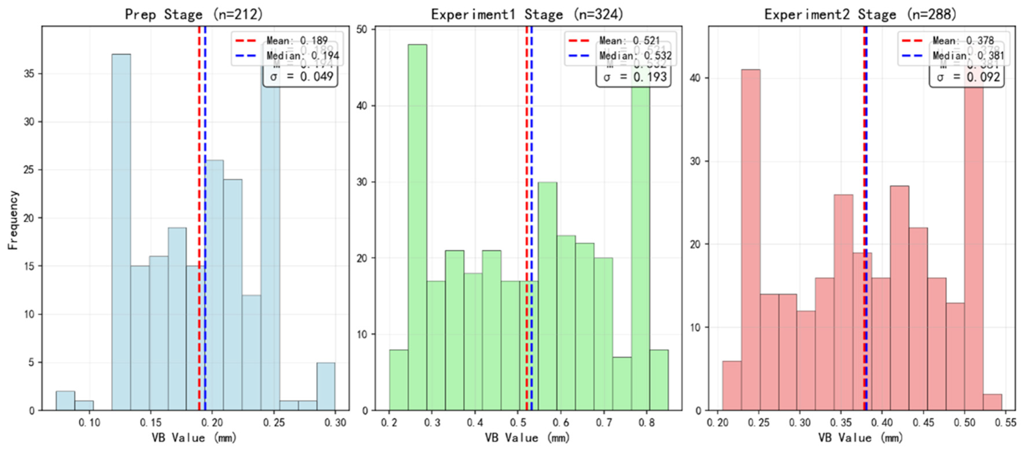
Finally, the stage distribution of VB values, as shown in Figure 7, is grouped by Prep, Experiment 1, and Experiment 2, capturing the frequency distribution, statistical features, and evolution trajectory of VB wear values. This enables the identification of the early run-in zone, fluctuation differences, and the potential impact of experimental conditions on the tool degradation process, providing a basis for segmented optimization.

4.2.3. Risk Intervals and Failure Early Warning Division

Utilizing the dynamic phases of time-series trends to map VB risk levels, a model is constructed through distribution plots, survival curves, and hazard rate curves, supporting GNN risk graph prediction and Transformer survival sequences. Risk boundaries can be incorporated into the loss function, enhancing the model’s accuracy in high-risk zones.

Firstly, the RUL distribution plot corresponding to segmented VB values, as shown in Figure 8, visually compares the RUL differences under different wear intervals, thereby providing quantitative support for predictive maintenance decisions. Specifically, the horizontal axis divides the VB wear categories for segmented evaluation of degradation degree; the vertical axis represents the RUL, reflecting the expected period from the equipment’s current state to failure.

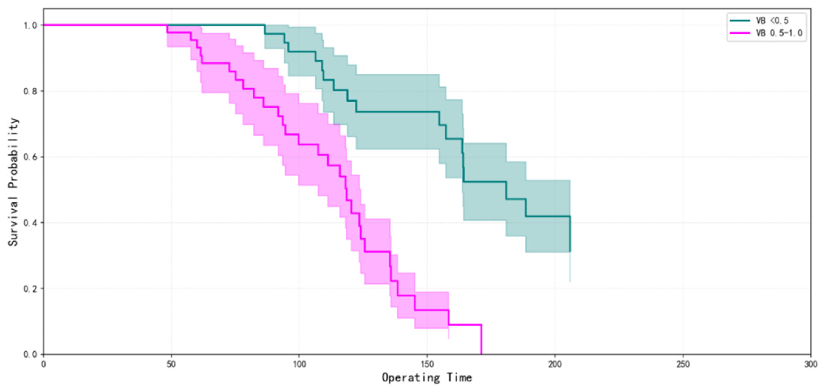
Secondly, the Kaplan–Meier survival analysis, as shown in Figure 9, clearly demonstrates the failure trends of different VB groups by estimating the survival probabilities in each interval. Among them, the curve for the VB ≤ 0.5 group declines relatively slowly, with early steps showing intermittent characteristics, and by about 200 units, the survival probability drops to about 0.4, indicating that this group has a higher long-term survival rate. In contrast, the curve for the VB 0.5–1.0 group declines steeply, with multiple steps occurring continuously, and by about 150 units, the survival probability drops to about 0.1, and finally drops to zero at about 170 units, reflecting a higher early failure risk. The obvious separation of the two curves verifies the effectiveness of VB as a risk factor. These early warning boundaries provide a risk-sensitive semantic foundation for multimodal dimensionality reduction.

4.2.4. Multimodal Interpretation and Dimensionality Reduction

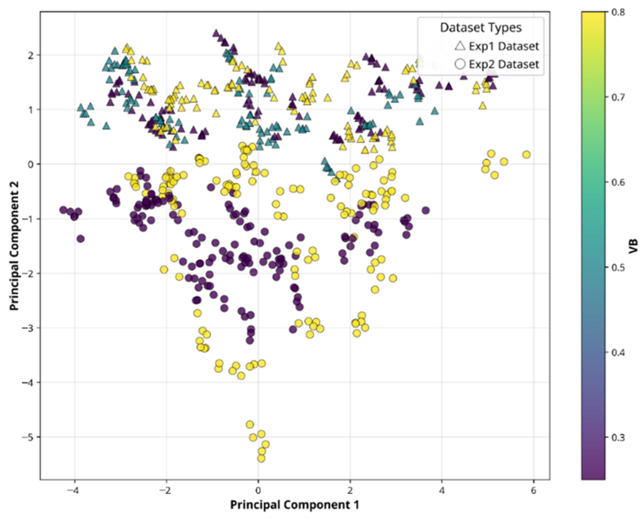
Based on the latent structures of risk intervals, latent semantic structures of multivariate data are revealed through Principal Component Analysis (PCA), demonstrating the clustering trends and interaction strengths of VB. To provide deeper insights into the machining context, PCA is employed to uncover the underlying patterns in multimodal data, including VB, cutting forces (Fx, Fy, Fz), surface roughness parameters (Ra, Rz, Rsk, Rku, RSm, Rt), and operational conditions. By analyzing the loadings of the principal components, we can infer their physical significance in the context of tool degradation. Firstly, the PCA dimensionality reduction plot, as shown in Figure 10, displays the distribution of multivariate data in a two-dimensional space, where the horizontal axis Principal Component 1 (PC1) captures the direction of maximum variance in the data, which typically corresponds to the core factors dominating the overall pattern. In this study, PC1 is found to be strongly correlated with VB and cutting force component Fx, suggesting that it primarily represents the overall tool wear progression, as VB is the dominant indicator of degradation and Fx exhibits a strong positive correlation with VB. Secondly, the vertical axis Principal Component 2 (PC2) is orthogonal to PC1, capturing secondary but independent variation patterns. PC2 is observed to be more closely associated with surface roughness parameters and operational conditions, reflecting variations in machining quality and process conditions that are less directly tied to wear progression.

Figure 10 illustrates the scatter plot of the dataset projected onto the PC1-PC2 plane, with data points color-coded by VB values to highlight the gradient of tool wear. The plot reveals distinct clustering trends, where data points with low VB values (indicating early-stage wear) are concentrated in the lower-left quadrant, while those with high VB values (indicating severe wear) shift toward the upper-right quadrant. This gradient distribution confirms VB’s pivotal role in driving the data variance captured by PC1. Additionally, the spread along PC2 suggests variability in surface quality and machining conditions, with tighter clusters indicating consistent machining outcomes and dispersed points reflecting condition-specific variations. This plot not only highlights the gradient influence of VB but also provides an intuitive basis for subsequent model optimization and semantic mining, supporting GNNs embedding initialization and Transformer semantic extraction. Specifically, the low-dimensional representations derived from PCA serve as compact inputs for the GNNs, enabling efficient initialization of node embeddings by capturing the dominant wear-related patterns in PC1 and condition-related patterns in PC2. For the Transformer, these representations enhance semantic extraction by providing a simplified yet informative feature space that preserves critical multimodal interactions.

The conclusions drawn from the PCA results are twofold. First, the strong alignment of PC1 with VB and Fx underscores the suitability of VB as a core degradation indicator, validating its use in graph construction and feature fusion within the proposed model. Second, the separation along PC2 highlights the importance of incorporating surface roughness and operational parameters in multimodal fusion, as these factors contribute to the variability in tool performance and machining outcomes. These insights guide the optimization of the GNNs-Transformer architecture by ensuring that both wear progression and contextual factors are adequately captured, thereby enhancing the efficiency and robustness of multimodal fusion in the RUL prediction task. The low-dimensional representations serve as inputs, enhancing the efficiency of multimodal fusion.

4.2.5. Predictive Performance and Uncertainty Assessment

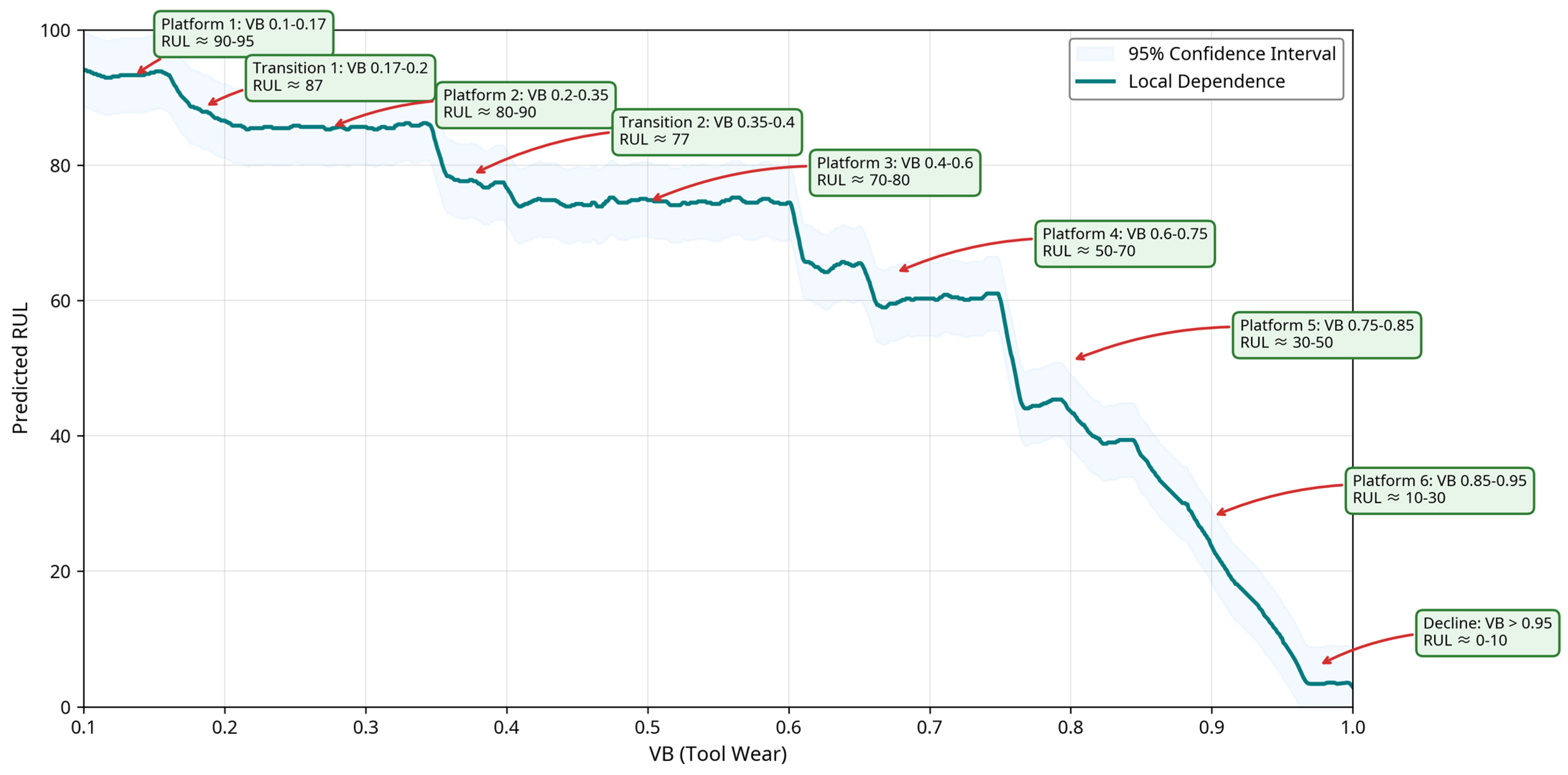
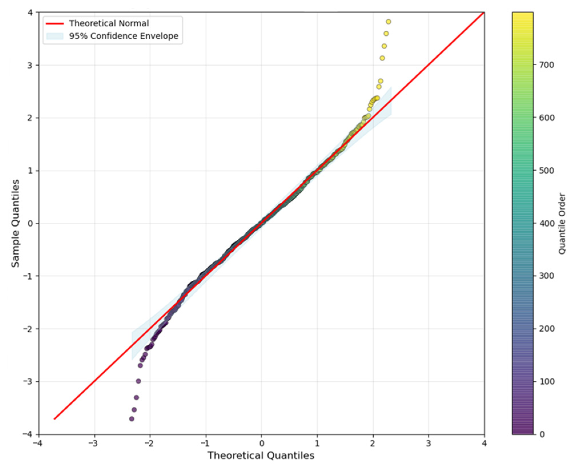
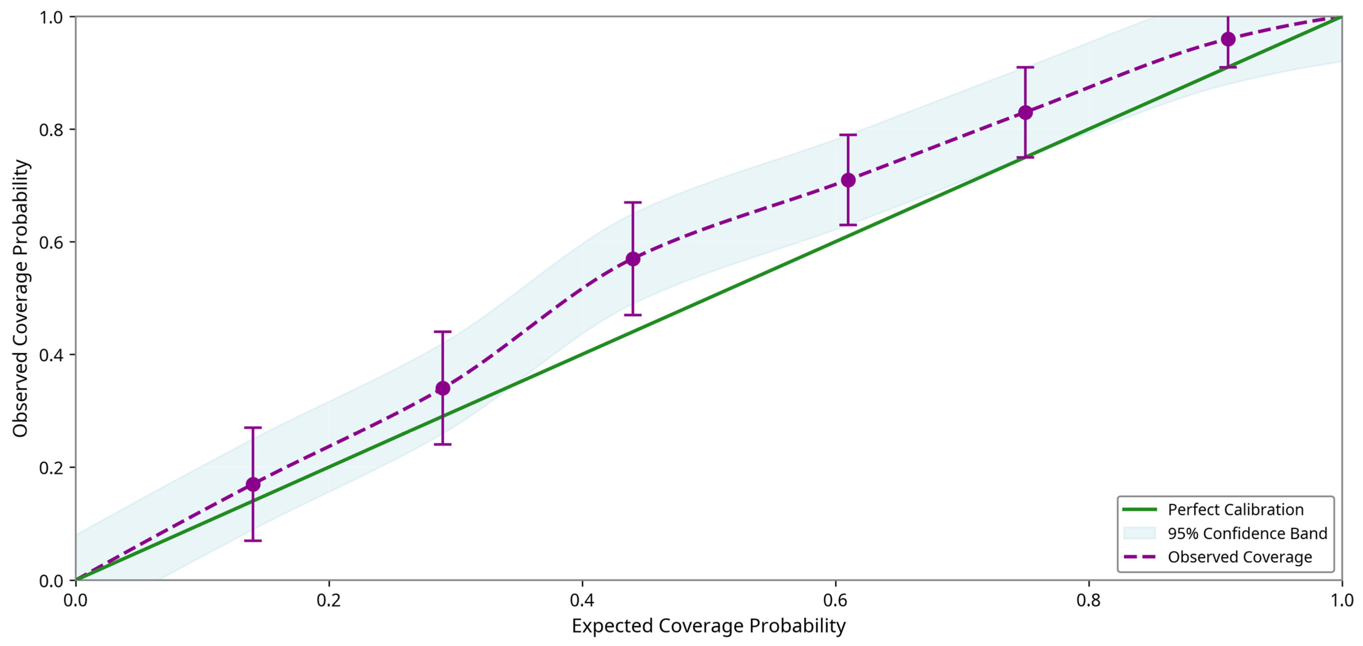
Integrating the reduced-dimensional features, the stability, confidence, and residuals of the GNNs-Transformer Model predictions are assessed through visualization, employing partial dependence plot, Quantile–Quantile Plot (QQ plot), and calibration curves to examine the response dominated by VB, distribution deviations, and coverage probabilities.

Firstly, the partial dependence plot, as shown in Figure 11, displays a nonlinear negative correlation trend. Specifically, as VB gradually increases, the predicted RUL exhibits multi-level plateau stages and transition stages, ultimately declining sharply in the high VB zone. The confidence interval is narrower in the low VB zone, while significantly widening in the high VB zone, reflecting increased uncertainty due to data sparsity.

Secondly, in the process of diagnosing the distribution of model prediction residuals, this study employs the Q-Q plot, as shown in Figure 12, to assess whether the residuals conform to the normal distribution assumption, by comparing the quantiles of the ordered residual samples with the theoretical quantiles of the standard normal distribution to achieve an ideal fit. The QQ plot exhibits an “S”-shaped deviation, with both ends exceeding the 95% confidence band, indicating heavy tails and asymmetric distribution, suggesting that the model fit is insufficient and requires improvement.

Finally, the reliability calibration plot, as shown in Figure 13, examines the coverage probability. It is used to check whether the coverage probability of the predicted confidence intervals matches the expected probability, that is, to evaluate the model’s calibration degree, by comparing the observed coverage probability with the expected coverage probability. In an ideal calibration state, the observed curve should closely fit the diagonal calibration line for perfect calibration, indicating that the model’s confidence intervals accurately reflect the true uncertainty. In this study, the observed curve is overall close to the calibration line, but slightly higher than expected in the medium to high expected zones, with the deviation indicating conservative intervals, stemming from overestimation of uncertainty.

4.2.6. Failure Classification and Determination Accuracy

Based on uncertainty assessment, the RUL health states are divided into healthy, warning, and failure categories, constructing judgments through predicted and actual line plots and accuracy analysis plots, examining the accuracy and offset of wear levels.

Firstly, in the dynamic comparative assessment of model performance, the focus is on analyzing the VB predicted values and actual measured values. Figure 14 presents a comparative analysis of actual VB values and predicted VB values across measurement points for three representative tools with different prediction performance levels: Tool 23 (good performance), Tool 13 (average performance), and Tool 41 (poor performance). This stratified representation reveals the model’s prediction capabilities across different wear conditions, with performance metrics (MSE, MAE) quantifying the prediction accuracy for each tool. The comparison enables insight into how prediction quality varies with wear severity and tool-specific characteristics.

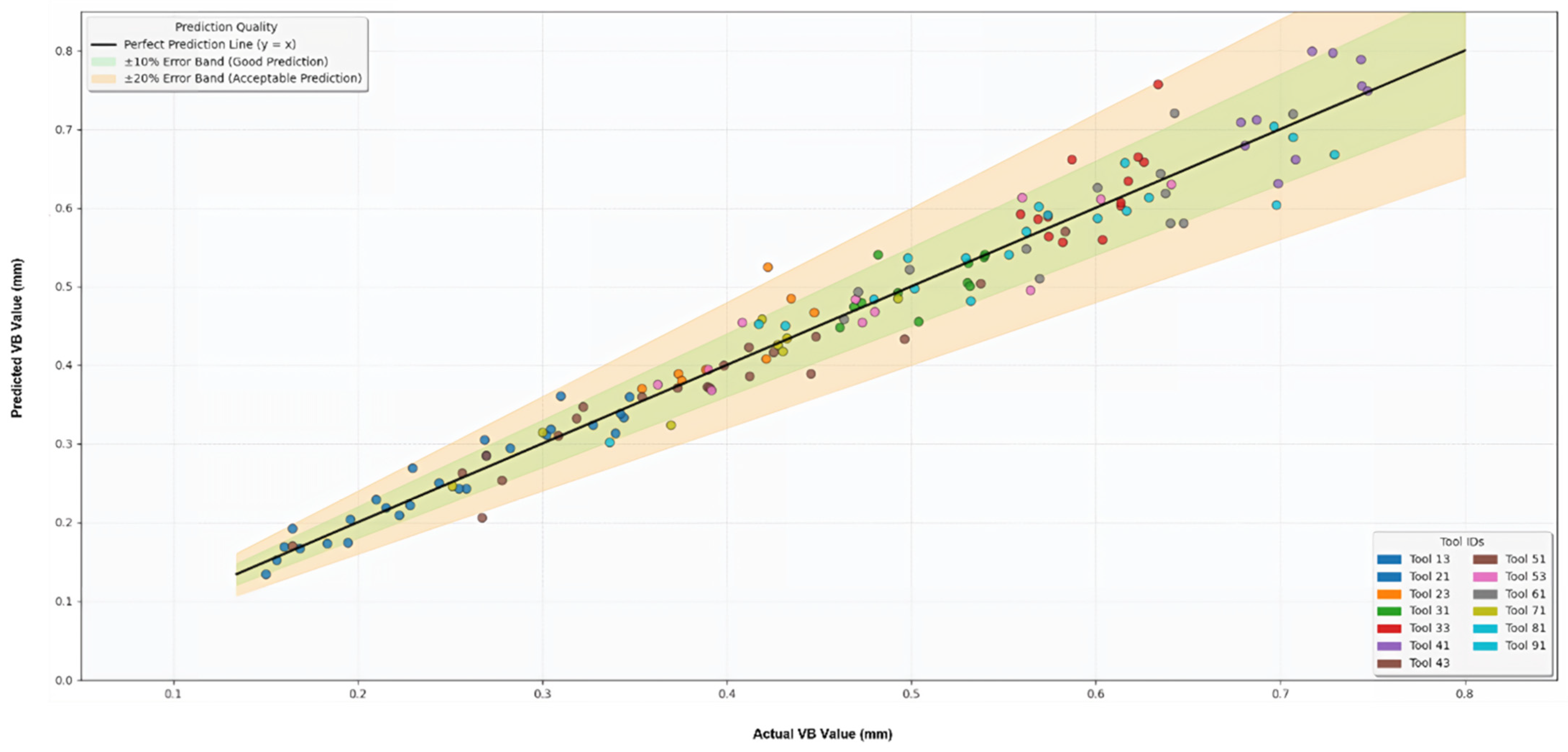
Secondly, the VB prediction accuracy analysis plot, as shown in Figure 15, displays performance through scatter points. Most points are distributed along the perfect line; the ±10% error band (good predictions) covers most points, the ±20% error band (acceptable predictions) includes a few points; very few points are outside the bands. The distribution for different Tool_IDs evaluates performance, with errors slightly increasing as VB increases.

4.2.7. Performance Comparison of Different Models

①

Evaluation Metrics

To evaluate the performance of the proposed model in the tool RUL prediction task, five standard metrics are used: mean squared error (MSE), mean absolute error (MAE), R² Score, accuracy, and F1-Score. These metrics assess the model’s regression performance for predicting continuous RUL values and classification performance for determining tool health states. Detailed definitions and formulations of these metrics can be found in the established machine learning literature [43,44].

②

Performance Comparison of Different Models

In order to further quantify the performance advantages of this model in the RUL prediction task and compare it with existing typical methods, this study selected LSTM-SVM, LSTM-CNN, and LSTM-XGBoost as benchmark models. These models were chosen as they are common benchmarks in the tool RUL prediction literature, representing diverse categories of solutions: LSTM-SVM combines recurrent networks with kernel-based methods for robust handling of sequential data; LSTM-CNN integrates convolutional and recurrent layers for spatiotemporal feature extraction; and LSTM-XGBoost leverages ensemble boosting for enhanced generalization across conditions, allowing a comprehensive evaluation against established hybrid approaches. These models represent common combinations of time-series processing with traditional machine learning or ensemble learning. Through experimental evaluations on the same dataset, the performance of each model was compared on regression and classification metrics.

Table 1. Model performance comparison.

Model	MSE	MAE	R2 Score	Accuracy	F1-Score
LSTM-SVM	0.086	0.049	0.823	0.809	0.781
LSTM-CNN	0.080	0.045	0.842	0.827	0.808
LSTM-XGBoost	0.069	0.042	0.876	0.854	0.836
Proposed Model	0.051	0.028	0.925	0.906	0.892

shows the performance comparison of four models in the tool RUL prediction task. These models include LSTM-SVM, LSTM-CNN, LSTM-XGBoost, and the Proposed GNNs-Transformer Model. The evaluation metrics include MSE, MAE, R² Score, accuracy, and F1-Score. These metrics comprehensively evaluate the models’ performance in regression tasks for predicting continuous RUL values and classification tasks for tool health status, such as healthy, warning, or failure states. Specifically, the main features of the LSTM-SVM model lie in the good robustness from the combination of sequential LSTM with SVM classification, but its limitations include high hybrid complexity and the need for parameter optimization; the features of the LSTM-CNN model are the fusion of time series and spatial features, which improves accuracy, but time–frequency limitations lead to weak relationship modeling; the features of the LSTM-XGBoost model are the combination of time series with ensemble learning, adaptable to multiple working conditions, but requiring generalization verification; the features of the Proposed GNNs-Transformer Model are multimodal fusion, graph relationship inference, and multi-task learning, with overall performance superior to the other models.

To ensure reproducibility and transparency in the experimental setup, the key hyperparameters for each benchmark model were optimized based on standard practices, using a validation subset of the dataset. The benchmark models were trained using the Adam optimizer with a learning rate of 1 × 10⁻³, batch size of 32, and early stopping after 20 epochs without improvement. For the LSTM-SVM model, the LSTM component consisted of two layers with 128 hidden units, followed by an SVM regressor/classifier using a radial basis function (RBF) kernel, regularization parameter C = 1.0, and gamma = 0.1. The LSTM-CNN model integrated 1D-CNN layers (three layers, kernel size = 5, filters = [64, 128, 256]) with a bidirectional LSTM (two layers, 128 hidden units), using ReLU activation and dropout = 0.2. The LSTM-XGBoost model employed a single LSTM layer (128 hidden units) to extract time-series features, which were then fed into XGBoost with 100 estimators, maximum depth = 6, learning rate = 0.1, and subsample = 0.8. For the Proposed GNNs-Transformer Model, as detailed in Section 3. These configurations were selected to balance computational efficiency and performance while ensuring fair comparison across models.

5. Discussion

This study proposes a tool RUL prediction model based on GNNs and Transformer optimization. While prior work has explored GNNs for leveraging equipment structures in RUL estimation, our novelty lies in the seamless integration of GNNs with Transformers via a specialized multimodal fusion strategy—combining dedicated encoders for diverse data types, GAT for relational inference, and a cross-modal Transformer decoder for deep interactions—coupled with a dual-head multi-task output for simultaneous RUL regression and health state classification, enabling more refined predictive maintenance beyond single-task paradigms. Through multimodal data fusion, graph adaptive relationship inference, and multi-task learning, it achieves precise evaluation and prospective prediction of tool health status. The experimental results validate the effectiveness of the model in aspects such as static correlation analysis, segmented trend modeling, risk interval division, multimodal interpretation, prediction performance evaluation, and failure classification. Moreover, they highlight VB’s multi-dimensional value as the core degradation indicator, extending beyond basic correlations to inform a closed-loop validation framework that integrates data exploration, model verification, and application optimization—ensuring the model’s comprehensiveness and robustness without reiterating module details.

This study broadens GNNs and Transformer applications in data processing by explicitly modeling entity relationships and enabling collaborative RUL regression and state classification, revealing wear turning points and providing a new framework for physics-guided deep learning, where “physics-guided” refers to the incorporation of domain-specific physical proxies like VB, derived from tool geometry and wear mechanics, into the fusion architecture, constraining the model to respect real-world degradation dynamics rather than purely data-driven patterns. Relative to mechanism-based models, it circumvents assumption limitations through data-driven multimodal fusion for superior generalization; compared to traditional machine learning, it minimizes feature engineering needs via GATs, outperforming ensembles in multivariable interaction capture. Benchmark comparisons underscore these gains in error control, fit, and classification, affirming the model’s innovative fusion and inference value. While the proposed model excels in accuracy, its computational cost must be considered for industrial feasibility. Training the full GNNs-Transformer architecture on an NVIDIA RTX 3090 GPU (24 GB memory) takes approximately 2.5 h per run, with inference time per sample around 50–100 ms, depending on batch size. In comparison, benchmark models like LSTM-SVM and LSTM-XGBoost require 30–60% less training time (1–1.5 h) due to simpler architectures, though they sacrifice multimodal depth. This higher cost stems from the GAT layers and Transformer decoder’s attention mechanisms, which process complex graph and sequence data. For industrialization, the model’s deployment in real-time CNC systems could be viable on edge devices with optimizations, but current complexity may limit scalability in resource-constrained environments; future lightweighting could reduce inference latency by 20–40% without significant accuracy loss, enhancing practical applicability in smart manufacturing.

The uncertainty assessment utilizing partial dependence plots represents an initial step toward model interpretability by visualizing VB’s nonlinear influence on RUL predictions. This aligns with the broader Explainable Artificial Intelligence (XAI) paradigm, which emphasizes transparency and trust in black-box models like GNNs and Transformers, particularly in high-stakes manufacturing where opaque decisions could lead to costly failures or safety risks. By integrating XAI techniques, such as SHapley Additive exPlanations (SHAP) values for feature attribution and ablation for modality contributions, the model not only quantifies uncertainty but also elucidates decision pathways, fostering user confidence in predictive maintenance systems. This approach is consistent with recent advances in developing physically interpretable, data-driven models. In manufacturing contexts, XAI techniques such as SHAP have been employed to analyze machine learning models for cavity prediction in electrochemical machining, effectively linking model behavior to process-level understanding and supporting anomaly detection [45]. In the wider XAI context for manufacturing, this work contributes to bridging the gap between complex AI and domain experts, enabling better integration with physics-guided models defined here as hybrids that embed physical proxies such as wear metrics into neural architectures for enhanced explainability. Influential future directions could include developing real-time XAI frameworks for edge-deployed systems, leveraging counterfactual explanations to simulate “what-if” scenarios in tool wear, or exploring federated XAI in multi-factory settings to preserve data privacy while aggregating insights across distributed CNC environments—ultimately advancing trustworthy AI for Industry 4.0 applications.

Although multimodal fusion remains the model’s key strength, VB indeed plays a central role as the core degradation indicator in both modeling and analysis, as it directly quantifies tool wear and serves as a proxy for integrating other modalities. However, to mitigate the risk of the approach devolving into a VB-centric regression rather than a truly multimodal system, we conducted feature importance analysis as

Table 2. Feature importance analysis.

Modality Category	Main Features	Importance (%)	Main Role Description
Geometric Wear Indicators	VB (flank wear width)	45%	Core degradation indicator that directly quantifies tool wear
Time-Series Signals	Fx/Fy/Fz (cutting forces, dominated by Fx)	25%	Capture variations in tool load and dynamic interactions
Surface Roughness Features	Ra, Rz, Rt, etc.	15%	Reflect machining quality and tool condition changes
Operational Parameters	Cutting depth, speed, feed rate, etc.	10%	Represent the influence of machining process conditions on wear
Experimental Phase Context	Experimental phases (Prep/Exp1/Exp2)	5%	Enhance cross-batch generalization and phase recognition ability

and ablation experiments as

Table 3. Ablation experiments.

Removed Modality	Main Included Features	Performance Change	Impact Description
Time-Series Signals	Fx, Fy, Fz	MSE ↑ 18%, Accuracy ↓ 9%	Missing cutting force signals weakens the model’s ability to capture dynamic variations
Geometric Data (excluding VB)	Tool diameter, etc.	MAE ↑ 12%	Loss of supplementary geometric wear information
Operational Parameters	Cutting depth, speed, feed rate	R2 ↓ 7%	Reduces the model’s adaptability to different machining conditions
Experimental Phase Context	Experimental phase information	F1-Score ↓ 6%	Decreases cross-phase recognition and generalization performance

to empirically validate the contributions of each modality (time-series signals like cutting forces Fx/Fy/Fz, geometric data including diameters, operational parameters such as cutting depth/speed/feed rate, and phase contexts like experimental batches). Using SHAP [46] values in the feature importance analysis, VB accounted for approximately 45% of the overall importance in RUL prediction, while cutting forces and surface roughness parameters contributed significantly to capturing dynamic interactions and machining quality variations; operational parameters and phase contexts added 10% and 5%, respectively, enhancing cross-batch generalization.

Ablation experiments, where individual modalities were removed and the model retrained on the same dataset, showed performance degradation: removing time-series data increased MSE by 18% and reduced accuracy by 9%; excluding geometric data (beyond VB) raised MAE by 12%; omitting operational parameters decreased R² by 7%; and ablating phase contexts lowered F1-Score by 6%. Surface roughness features (Ra, Rz, Rt, etc.) are integrated into the geometric feature stream; therefore, their ablation effect is collectively represented under “Geometric Data (excluding VB)” rather than treated as a separate modality.

These results confirm that while VB is pivotal, the multimodal fusion leverages complementary information from all sources, preventing over-reliance on a single indicator and ensuring robust predictions in diverse conditions.

Despite these advancements, limitations persist: the model’s reliance on VB may undervalue noise in industrial settings, potentially biasing predictions; furthermore, the study does not demonstrate generalization across different tools or materials, as evaluations were confined to the specific dataset of 13 tools under controlled conditions, limiting insights into broader applicability; high computational demands further constrain real-time deployment. Future efforts should diversify datasets for broader conditions, integrate additional modalities to lessen VB dependence, and apply lightweighting techniques like pruning or quantization to optimize for edge computing, balancing accuracy with practicality.

6. Conclusions

In this paper, an innovative cutting tool RUL prediction model based on GNNs and Transformer optimization is presented for effectively addressing the core challenges of multimodal data fusion, complex relationship modeling, and task singularity. The modeling approach can finely process multimodal features through dedicated encoders, explicitly capture non-Euclidean structural dependencies using GATs, generates fused contextual features via a cross-modal Transformer decoder, and ultimately render collaborative prediction of RUL regression and health status classification of cutting tools with dual-head outputs.

The key conclusions of this study are summarized in the following points:

1. The proposed GNNs-Transformer architecture innovatively integrates multimodal encoding, graph adaptive fusion via GATs, and cross-modal Transformer decoding, enabling deep interaction across time-series signals, geometric data, operational parameters, and phase contexts, while the dual-head multi-task output simultaneously handles RUL regression and health state classification, overcoming limitations of shallow fusion and single-task models.

2. Experiments on a multimodal dataset of 824 entries, structured across 13 tools with 4–6 measurements each and split into 70% training, 15% validation, and 15% independent testing, validate the model’s efficacy through a systematic framework including correlation analysis, trend modeling, risk assessment, and uncertainty quantification.

3. VB emerges as the core degradation indicator, with analyses confirming its strong negative correlation with RUL, nonlinear temporal evolution, risk threshold potential, and robust performance in failure classification, supported by critical evaluations such as residual diagnostics revealing minor mid-range biases and heteroscedasticity.

4. The model outperforms benchmarks (LSTM-SVM, LSTM-CNN, LSTM-XGBoost) by 26–41% in MSE, 33–43% in MAE, 6–12% in R², 6–12% in accuracy, and 7–14% in F1-Score, verified through feature importance (VB at 45%, others complementary) and ablation studies demonstrating each modality’s essential role.

5. Overall, this architecture enhances prediction accuracy, robustness, and decision guidance for predictive maintenance in smart manufacturing, with future directions including dataset expansion, further modality integration, lightweighting for edge deployment, and advanced XAI for real-time interpretability in Industry 4.0.

References

1. Cheng, K.; Niu, Z.C.; Wang, R.C.; Rakowski, R.; Bateman, R. Smart cutting tools and smart machining: Development approaches, and their implementation and application perspectives. Chin. J. Mech. Eng. 2017, 30, 1162–1176. [Google Scholar] [CrossRef]
2. Yao, K.C.; Chen, D.C.; Pan, C.H.; Lin, C.L. The development trends of computer numerical control (CNC) machine tool technology. Mathematics 2024, 12, 1923. [Google Scholar] [CrossRef]
3. Zhou, Y.; Liu, C.; Yu, X.; Liu, B.; Quan, Y. Tool wear mechanism, monitoring and remaining useful life (RUL) technology based on big data: A review. SN Appl. Sci. 2022, 4, 232. [Google Scholar] [CrossRef]
4. Zonta, T.; da Costa, C.A.; da Rosa Righi, R.; de Lima, M.J.; da Trindade, E.S.; Li, G.P. Predictive maintenance in the Industry 4.0: A systematic literature review. Comput. Ind. Eng. 2020, 50, 106889. [Google Scholar] [CrossRef]
5. Sayyad, S.; Kumar, S.; Bongale, A.; Kamat, P.; Patil, S.; Kotecha, K. Data-driven remaining useful life estimation for milling process: Sensors, algorithms, datasets, and future directions. IEEE Access 2021, 9, 110255–110286. [Google Scholar] [CrossRef]
6. Achouch, M.; Dimitrova, M.; Ziane, K.; Karganroudi, S.S.; Dojcinovski, D.; Ibrahim, A.M.; Adda-Bedia, E.A. On predictive maintenance in industry 4.0: Overview, models, and challenges. Appl. Sci. 2022, 12, 8081. [Google Scholar] [CrossRef]
7. Tsanousa, A.; Bektsis, E.; Kyriakopoulos, C.; González, A.G.; Karakostas, A.; Stavropoulos, G.; Vrochidis, S. A review of multisensor data fusion solutions in smart manufacturing: Systems and trends. Sensors 2022, 22, 1734. [Google Scholar] [CrossRef]
8. Narwariya, J.; Malhotra, P.; Vig, L.; Shroff, G.; Vishnu, T.V. Graph neural networks for leveraging industrial equipment structure: An application to remaining useful life estimation. arXiv 2020, arXiv:2006.16556. [Google Scholar] [CrossRef]
9. Zhu, K.; Li, X.; Li, S.; Lin, X. Physics-informed hidden markov model for tool wear monitoring. J. Manuf. Syst. 2024, 72, 308–322. [Google Scholar] [CrossRef]
10. Zhu, K.; Huang, C.; Li, S.; Lin, X. Physics-informed Gaussian process for tool wear prediction. ISA Trans. 2023, 143, 548–556. [Google Scholar] [CrossRef]
11. Ertunc, H.M.; Loparo, K.A.; Ocak, H. Tool wear condition monitoring in drilling operations using hidden Markov models (HMMs). Int. J. Mach. Tools Manuf. 2001, 41, 1363–1384. [Google Scholar] [CrossRef]
12. Wang, Y.; Chang, M.; Huang, X.; Li, Y.; Tang, J. Cutting tool wear prediction based on the multi-stage Wiener process. Int. J. Adv. Manuf. Technol. 2023, 129, 5319–5333. [Google Scholar] [CrossRef]
13. Liu, W.C.; Yang, W.A.; You, Y.P. Three-Stage Wiener-Process-Based Model for Remaining Useful Life Prediction of a Cutting Tool in High-Speed Milling. Sensors 2022, 22, 4763. [Google Scholar] [CrossRef] [PubMed]
14. Li, Y.; Huang, X.; Tang, J.; Li, S.; Ding, P. A steps-ahead tool wear prediction method based on support vector regression and particle filtering. Measurement 2023, 218, 113237. [Google Scholar] [CrossRef]
15. Cheng, Y.N.; Gai, X.Y.; Jin, Y.B. A new method based on a WOA-optimized support vector machine for tool wear prediction. Int. J. Adv. Manuf. Technol. 2022, 121, 4993–5012. [Google Scholar] [CrossRef]
16. Qin, X.; Huang, W.; Wang, X.; Tang, Z.; Liu, Z. Real-Time Remaining Useful Life Prediction of Cutting Tools Using Sparse Augmented Lagrangian Analysis and Gaussian Process Regression. Sensors 2023, 23, 413. [Google Scholar] [CrossRef]
17. Huang, Z.; Shao, J.; Guo, W.; Li, W.; Zhu, J.; He, Q. Tool Wear Prediction Based on Multi-Information Fusion and Genetic Algorithm-Optimized Gaussian Process Regression in Milling. IEEE Trans. Instrum. Meas. 2023, 72, 2516716. [Google Scholar] [CrossRef]
18. Airao, J.; Gupta, A.; Nirala, C.K.; Hsue, A.W.J. Bayesian neural networks modeling for tool wear prediction in milling Al 6061 T6 under MQL conditions. Int. J. Adv. Manuf. Technol. 2024, 135, 2777–2788. [Google Scholar] [CrossRef]
19. Dong, J.; Subrahmanyam, K.V.R.; Wong, Y.S.; Hong, G.S.; Mohanty, A.R. Bayesian-inference-based neural networks for tool wear estimation. Int. J. Adv. Manuf. Technol. 2006, 29, 811–818. [Google Scholar] [CrossRef]
20. Truong, T.T.; Airao, J.; Hojati, F.; Ilvig, C.F.; Azarhoushang, B.; Karras, P.; Aghababaei, R. Data-driven prediction of tool wear using Bayesian regularized artificial neural networks. Measurement 2024, 238, 115303. [Google Scholar] [CrossRef]
21. Cardoz, B.; Shaikh, H.; Mulani, S.; Kumar, A.; Sabareesh, G. Random forests based classification of tool wear using vibration signals and wear area estimation from tool image data. Int. J. Adv. Manuf. Technol. 2023, 126, 3069–3081. [Google Scholar] [CrossRef]
22. Cheng, Y.N.; Zhou, S.L.; Xue, J. Research on tool wear prediction based on the random forest algorithm optimized by the northern goshawk optimization algorithm. Mach. Sci. Technol. 2024, 28, 456–478. [Google Scholar] [CrossRef]
23. Chen, S.Y.; Yin, Z.B.; Zhang, L.; Yuan, J. Study of an ISSA-XGBoost model for milling tool wear prediction under variable working conditions. Int. J. Adv. Manuf. Technol. 2024, 133, 2761–2774. [Google Scholar] [CrossRef]
24. Alajmi, M.S.; Almeshal, A.M. Predicting the Tool Wear of a Drilling Process Using Novel Machine Learning XGBoost-SDA. Materials 2020, 13, 4952. [Google Scholar] [CrossRef] [PubMed]
25. Bustillo, A.; Urbikain, G.; Perez, J.M.; Pereira, O.M.; de Lacalle, L.N.L. Smart optimization of a friction-drilling process based on boosting ensembles. J. Manuf. Syst. 2018, 48 Pt C, 108–121. [Google Scholar] [CrossRef]
26. Letot, C.; Serra, R.; Dossevi, M.; Dehombreux, P. Cutting tools reliability and residual life prediction from degradation indicators in turning process: A case study involving four approaches. Int. J. Adv. Manuf. Technol. 2016, 86, 495–506. [Google Scholar] [CrossRef]
27. Bergs, T.; Holst, C.; Gupta, P.; Augspurger, T. Digital image processing with deep learning for automated cutting tool wear detection. Procedia Manuf. 2020, 48, 947–958. [Google Scholar] [CrossRef]
28. García-Pérez, A.; Ziegenbein, A.; Schmidt, E.; Shamsafar, F.; Fernández-Valdivielso, A.; Llorente-Rodríguez, R.; Weigold, M. CNN-based in situ tool wear detection: A study on model training and data augmentation in turning inserts. J. Manuf. Syst. 2023, 68, 85–98. [Google Scholar] [CrossRef]
29. Caggiano, A.; Mattera, G.; Nele, L. Smart tool wear monitoring of CFRP/CFRP stack drilling using autoencoders and memory-based neural networks. Appl. Sci. 2023, 13, 3307. [Google Scholar] [CrossRef]
30. Li, H.; Wang, W.; Li, Z.; Dong, L.; Li, Q. A novel approach for predicting tool remaining useful life using limited data. Mech. Syst. Signal Process. 2020, 143, 106832. [Google Scholar] [CrossRef]
31. De Barrena, T.F.; Ferrando, J.L.; García, A.; Badiola, X.; de Buruaga, M.S.; Vicente, J. Tool remaining useful life prediction using bidirectional recurrent neural networks (BRNN). Int. J. Adv. Manuf. Technol. 2023, 125, 4027–4045. [Google Scholar] [CrossRef]
32. Hassan, M.; Sadek, A.; Attia, M.H. A Generalized Multisensor Real-Time Tool Condition–Monitoring Approach Using Deep Recurrent Neural Network. Smart Sustain. Manuf. Syst. 2019, 3, 41–62. [Google Scholar] [CrossRef]
33. Bian, Q.; Wang, C.; Bo, C.; Peng, H.; Zhang, M. AE-LSTM-CNN Model based Tool Wear Monitoring. In Proceedings of the 2023 CAA Symposium on Fault, Supervision, and Safety for Technical Processes (SAFEPROCESS), Hangzhou, China, 22–24 September 2023; pp. 1–6. [Google Scholar] [CrossRef]
34. Lu, S.; Zhu, Y.; Liu, S.; She, J. A Tool Wear Prediction Model Based on Attention Mechanism and IndRNN. In Proceedings of the 2022 International Joint Conference on Neural Networks (IJCNN), Padua, Italy, 18–23 July 2022; pp. 1–8. [Google Scholar] [CrossRef]
35. Cetin, O.; Ostendorf, M.; Loparo, K.A. Multirate coupled hidden Markov models and their application to machining tool-wear classification. IEEE Trans. Signal Process. 2007, 556, 2885–2896. [Google Scholar] [CrossRef]
36. Assafo, M.; Langendoerfer, P. Tool remaining useful life prediction using feature extraction and machine learning-based sensor fusion. Results Eng. 2025, 28, 107297. [Google Scholar] [CrossRef]
37. Pang, B.; Yuan, D.; Li, D.; Di, Z. Tool Remaining Useful Life Prediction Method Based on Time-frequency Features Fusion and Long Short-term Memory Network. In Proceedings of the 2021 Global Reliability and Prognostics and Health Management (PHM-Nanjing), Nanjing, China, 15–17 October 2021; pp. 1–7. [Google Scholar] [CrossRef]
38. Si, S.; Mu, D.; Si, Z. Intelligent tool wear prediction based on deep learning PSD-CVT model. Sci. Rep. 2024, 14, 20754. [Google Scholar] [CrossRef]
39. Hao, C.; Mao, X.; Ma, T.; He, S.; Li, B.; Liu, H.; Peng, F.; Zhang, L. A novel deep learning method with partly explainable: Intelligent milling tool wear prediction model based on transformer informed physics. Adv. Eng. Inform. 2023, 57, 102106. [Google Scholar] [CrossRef]
40. Zhu, K.; Guo, H.; Li, S.; Lin, X. Physics-Informed Deep Learning for Tool Wear Monitoring. IEEE Trans. Ind. Inform. 2024, 20, 524–533. [Google Scholar] [CrossRef]
41. Sawangsri, W.; Cheng, K. An innovative approach to cutting force modelling in diamond turning and its correlation analysis with tool wear. Proc. IMechE Part B J. Eng. Manuf. 2016, 230, 405–415. [Google Scholar] [CrossRef]
42. Canal, A. CNC Turning: Roughness, Forces and Tool Wear. Kaggle, 2022. Available online: https://www.kaggle.com/datasets/adorigueto/cnc-turning-roughness-forces-and-tool-wear (accessed on 16 March 2025).
43. Rainio, O.; Teuho, J.; Klén, R. Evaluation metrics and statistical tests for machine learning. Sci. Rep. 2024, 14, 6086. [Google Scholar] [CrossRef]
44. Naidu, G.; Zuva, T.; Sibanda, E.M. A review of evaluation metrics in machine learning algorithms. In Lecture Notes in Networks and Systems, Proceedings of the Computer Science On-line Conference (CSOC 2023), Online, 3–4 April 2023; Springer: Berlin/Heidelberg, Germany, 2023; Volume 724, pp. 15–25. [Google Scholar] [CrossRef]
45. Wu, M.; Yao, Z.; Verbeke, M.; Karsmakers, P.; Gorissen, B.; Reynaerts, D. Data-driven models with physical interpretability for real-time cavity profile prediction in electrochemical machining processes. Eng. Appl. Artif. Intell. 2025, 160, 111807. [Google Scholar] [CrossRef]
46. Lundberg, S.M.; Lee, S.-I. A unified approach to interpreting model predictions. In Proceedings of the 31st Conference on Neural Information Processing Systems (NIPS’17), Long Beach, CA, USA, 4–9 December 2017; pp. 4768–4777. [Google Scholar]
Figure 1. Architecture for tool RUL calculation.
Machines 13 01027 g001
Figure 2. Residual analysis of VB and RUL.
Machines 13 01027 g002
Figure 3. Comparation of VB and Cutting Force Components.
Machines 13 01027 g003
Figure 4. VB and roughness multivariable correlation.
Machines 13 01027 g004
Figure 5. Degradation trajectory.
Machines 13 01027 g005
Figure 6. Nonlinear degradation.
Machines 13 01027 g006
Figure 7. VB value stage distribution.
Machines 13 01027 g007
Figure 8. RUL distribution corresponding to segmented VB values.
Machines 13 01027 g008
Figure 9. Kaplan–Meier survival analysis.
Machines 13 01027 g009
Figure 10. PCA dimensionality reduction.
Machines 13 01027 g010
Figure 11. Partial dependence plot.
Machines 13 01027 g011
Figure 12. Predicted residual QQ.
Machines 13 01027 g012
Figure 13. Reliability calibration.
Machines 13 01027 g013
Figure 14. VB predicted values and measured values.
Machines 13 01027 g014
Figure 15. VB prediction accuracy analysis.
Machines 13 01027 g015