Abstract
A collaborative control strategy combining the hyperbolic sine-cosine optimization (SCHO) algorithm with fuzzy adaptive linear active disturbance rejection control is proposed to address the nonlinearity and uncertainties in the hydraulic position servo system of shock absorber test benches. First, based on the dynamic characteristics of the shock absorber fatigue test bench and the tested shock absorber, a linearized model of the valve-controlled hydraulic cylinder and its load was established. The coupling mechanism of system parameter perturbation and disturbance was also analyzed. A third-order LADRC (Linear Active Disturbance Rejection Control) was designed considering the linear model characteristics of the test bench hydraulic servo system model to quickly estimate internal system disturbances and perform real-time compensation. Secondly, a multi-objective optimization function was constructed by integrating system performance indicators and incorporating controller and observer bandwidths into the optimization objectives. The SCHO algorithm was used for the global search and optimization of key LADRC parameters. To enhance the controller’s adaptive capability of modeling uncertainties and external disturbances, a fuzzy adaptive module was introduced to adjust control gains online according to errors and their rates of change, further improving system robustness and dynamic performance. The results show that compared with traditional PID, under different working conditions, the proposed method reduced the maximum tracking error, overshoot, and system response time by an average of 45%, from 15% to 5%, and by approximately 30%, respectively. Meanwhile, the parameter combination obtained via SCHO effectively avoids the limitations of manual parameter tuning, significantly improving control accuracy and energy utilization. The simulation results indicate that this method can significantly enhance position-tracking accuracy compared with traditional LADRC, providing an effective solution for position-tracking control in hydraulic servo testing systems.
1. Introduction
As a key component of the vehicle suspension system, damper performances directly affect driving safety, comfort, and stability. To ensure product quality, damper fatigue test benches are used to simulate real operating conditions and evaluate durability and damping characteristics [1]. Among them, the electro-hydraulic servo system serves as the core actuator, and its position-tracking accuracy and dynamic response critically determine the reliability of test results [2].
However, the electro-hydraulic servo system is inherently nonlinear and uncertain, which poses a significant challenge to controller robustness. Traditional PID control, though simple and widely used, heavily relies on accurate system models and lacks adaptability to nonlinear disturbances. In contrast, model-based adaptive controls enhance robustness by introducing nonlinear compensation, but the modeling complexity and computational cost hinder practical applications.
Recently, researchers worldwide have made efforts to improve the performance and energy efficiency of hydraulic servo systems. For instance, Righettini et al. [3] proposed a systematic management and control methodology for high energy saving in applications equipped with hydraulic servo-axes, achieving up to 88% energy efficiency improvement through load estimation and supply optimization. Their work reflects the growing global interest in both the control performance and sustainable operation of electro-hydraulic systems.
To address the issues of system nonlinearity and disturbances, scholars have explored a variety of advanced intelligent control strategies, such as extended observers [4], sliding-mode composite control [5], and intelligent algorithms [6]. Moreover, Sharifi et al. [7] introduced a nonlinear representation learning approach for leakage fault detection in electro-hydraulic servo systems, demonstrating the effectiveness of data-driven methods for modeling and fault diagnosis under nonlinear dynamics.
Among these, active disturbance rejection control offers a model-free alternative by estimating and compensating disturbances directly, making it particularly suitable for electro-hydraulic systems. The LADRC simplifies the standard ADRC (Active Disturbance Rejection Control) by reducing parameter complexity while preserving control performance, utilizing a tracking differentiator, extended state observer, and linear state error feedback. Recent applications include Liu’s LADRC [8] with dead zone compensation in weeding machinery and Jin’s LADRC [9] with acceleration feedforward for asymmetric cylinders.
In recent years, intelligent algorithms have been increasingly applied to electro-hydraulic servo systems to enhance control accuracy, adaptability, and robustness. For instance, intelligent PID controllers [10] have been developed for industrial electro-hydraulic systems to improve dynamic performance under varying conditions. Furthermore, model predictive control schemes optimized using advanced metaheuristic algorithms such as the cuckoo search [11] and genetic algorithms [12] have shown promising results in force tracking performance. Iterative learning control and observer-based sliding mode control have also been introduced for real-time implementation [13] and rapid response tracking in electro-hydraulic and hybrid systems. Hoang et al. [14] proposed a super-twisting observer-based integral sliding mode control, enabling high-precision acceleration tracking for a hybrid electro-hydraulic-pneumatic piston system. These studies demonstrate the effectiveness of combining intelligent optimization and adaptive control theories in improving the nonlinear dynamic characteristics of hydraulic servo systems.
Furthermore, intelligent algorithms like PSO (Particle Swarm Optimization) and GA (Genetic Algorithm) are widely used to optimize LADRC parameters such as observer and controller bandwidths due to their global search capabilities. For example, Ren [15] applied the Gray Wolf Optimizer to ADRC tuning, improving efficiency through intelligent group behavior. However, GWO can struggle with convergence in complex systems. To overcome this, Xiao [16] proposed a hybrid CGWO-PSO (Chaotic Gray Wolf Optimizer-Particle Swarm Optimization) algorithm for optimizing sliding mode parameters, while Ji [17] used adaptive neural networks for real-time uncertainty estimation and robust yaw control in vehicles. While traditional PID and model-based adaptive controls have their strengths, LADRC offers a compelling balance of simplicity and robustness, especially when combined with intelligent optimization algorithms for parameter tuning [18].
To further improve the adaptive capability of the controller, this paper introduced the fuzzy adaptive control strategy [19], used the hyperbolic sine cosine optimization algorithm to perform multi-objective optimization on key controller parameters, and constructed a fuzzy LADRC controller to achieve a balance between fast response and high-precision tracking.
The SCHO algorithm leverages the oscillatory characteristics of sine and cosine functions to balance global search and local convergence, often outperforming PSO and GA, providing an efficient means for LADRC parameter optimization [20]. Meanwhile fuzzy logic can nonlinearly adjust adaptive gains based on real-time states such as position error and error change rate, compensating for the limitations of fixed parameters. Combining the two enables “offline global optimization + online dynamic fine-tuning”—first using SCHO to determine optimal fixed parameters offline, then relying on fuzzy rules to correct adaptive gains online, thus balancing optimal static performance and real-time robustness.
2. Modeling Electro-Hydraulic Position Servo System
To conduct the design of the Linear Active Disturbance Rejection Controller (LADRC), a mathematical model of the valve-controlled cylinder system was established. However, considering the inherent nonlinear characteristics of the system, the effectiveness of this control strategy will be verified through the co-simulation of AMESIM and Simulink.
The system utilizes a three-position four-way valve and a symmetric hydraulic cylinder as its main power component, as shown in Figure 1. and are the area of the left and right cavity of the hydraulic cylinder, respectively; and are the pressure in the left and right chamber of the hydraulic cylinder, respectively; and are the flow in the left and right cavity of the hydraulic cylinder, respectively; is the total mass of the piston and the load converted to the piston; is the slide valve displacement; is the displacement of the piston rod of the hydraulic cylinder; is the oil supply pressure; is the oil return pressure.

Figure 1.
Schematic diagram of valve-controlled symmetric hydraulic cylinder.
The linearized flow equation of the servo valve is expressed as follows:
where is the load flow; is the flow gain of servo valve spool; is the flow-pressure gain coefficient; is the pressure drop.
The flow continuity equation of the hydraulic cylinder is expressed as follows:
where is the effective area of the hydraulic cylinder piston; is the elastic modulus of hydraulic oil; is the total leakage coefficient of hydraulic cylinder; is the total equivalent volume.
The force balance equation of the hydraulic cylinder and load is expressed as follows:
where is the viscous damping coefficient; is the equivalent elastic load stiffness; is the load force on the piston.
Based on Equations (1)–(3) and considering the inertial, viscous friction, and elastic loads, as well as the compressibility of oil and cylinder leakage, the actual system load is often simple. In the involved impact limiter test stand, the load types are mainly inertial and damping. With simplification, the piston displacement of the hydraulic cylinder is relative to the control valve opening.
The transfer function of is expressed as follows:
Natural frequency is calculated as follows:
The hydraulic damping ratio is calculated as follows:
where is the total flow-pressure coefficient.
The servo amplifier is generally handled according to the proportional link, with the following relationships:
where is the control voltage; is the control current of the servo valve; is the servo amplifier gain.
Due to the high response frequency of the servo valve, it is simplified into a proportional link and expressed as follows:
where , , is the no-load flow, gain, and the control current of the servo valve, respectively.
The control flowchart of the hydraulic servo valve control system was established according to the mathematical model of each part of the hydraulic servo system, as shown in Figure 2.
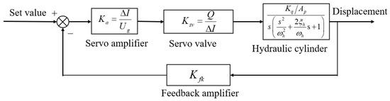
Figure 2.
Block diagram of the electro-hydraulic servo control system.
Figure 2 shows the linearized simplified model, while the actual system has nonlinear characteristics such as servo valve dead zone and Coulomb friction. These unmodeled dynamics are regarded as “total disturbance”, which is estimated online and compensated by the LESO of LADRC.
Establishing the Shock Absorber Model
The hydraulic shock absorber absorbs transient impacts and attenuates periodic vibrations through the synergistic action of elastic elements and damping elements. Its physical structure is shown in Figure 3, and its operating principle is as follows: when the piston rod is subjected to an external load force, the hydraulic oil pressure in the working chamber increases, pushing the isolation piston to move left and compressing the elastic medium on the left side, thereby generating an elastic force proportional to the displacement. At the same time, the high-pressure oil flows to the oil reservoir through the damping valve, and a damping force is formed by the viscous resistance of the oil flow. When the external force disappears, the elastic force drives the isolation piston to move right, and the oil in the oil reservoir is supplemented to the working chamber through the inlet valve, pushing the piston rod back to its initial state to complete automatic reset. Simplify Figure 3 into a spring-damper-mass system, as shown in Figure 4. This physical structure is a linear lumped-parameter simplification, which ignores nonlinear characteristics such as the internal influence of the shock absorber, friction, fluid inertia, etc., and only retains three key elements: equivalent mass , stiffness , and damping coefficient . It is used to analyze the influence of load dynamics on the valve-controlled cylinder system. It should be noted that the following model describes the shock absorber subsystem, which was analyzed independently from the hydraulic servo system shown in Figure 1.
where is the equivalent mass of the piston and connecting rod; is the equivalent damping coefficient; and is the equivalent spring stiffness.
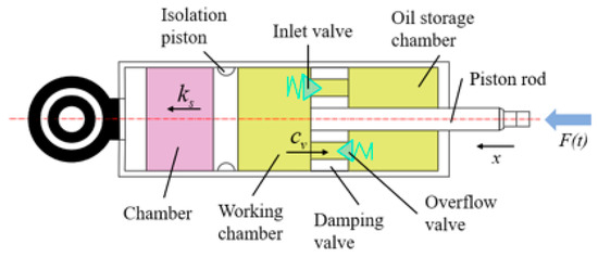
Figure 3.
Physical structure of the shock absorber.
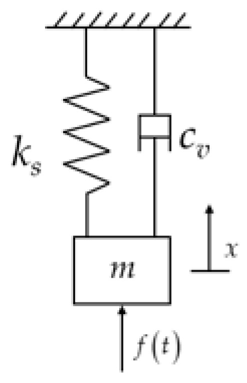
Figure 4.
Simplified spring damping model.
The simulation was based on the above system model. The parameter values were as follows: the equivalent mass m was 100 kg, and the equivalent stiffness ks was 10,000 N/m. To investigate the effect of damping coefficient on system response, the damping coefficients Cv were set to 1000, 2000, and 3000 N·s/m, respectively. Figure 5 presents the comparison results of the dynamic characteristics of the system displacement response under different damping conditions. Under the excitation response of a step input, the influence law of the damping ratio on the dynamic performance of the system was as follows: under low damping conditions, the response curve exhibited significant oscillation characteristics with a peak displacement of 0.25 m and continuous fluctuations within 5 s; under medium damping conditions, the overshoot decreased to 3.3%, and the settling time was shortened to approximately 4 s; under high damping conditions, there was no visible overshoot in the response, and it quickly converged to the steady-state value within 2.5 s. As the damping coefficient increased from 1000 N·s/m to 3000 N·s/m, the oscillation amplitude decreased by 60%, and the time for the system to enter the ±5% steady-state error band was reduced by 50%.
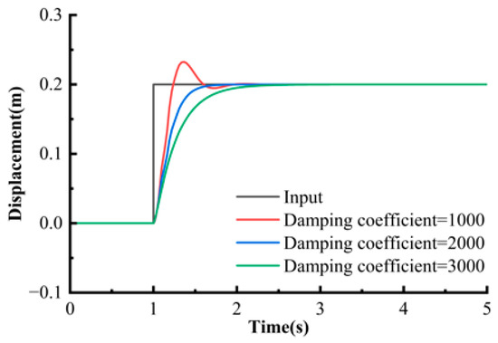
Figure 5.
Step responses with different damping coefficients.
3. Design of Three-Order Linear Automatic Disturbance Rejection Controller
Given the third-order integral nature of the electro-hydraulic servo system, a third-order LADRC was employed for precise displacement control [21]. The controller, illustrated in Figure 6, comprises a Linear Extended State Observer (LESO), a Linear State Error Feedback (LSEF), and a Linear Derivative Tracker (LDT).
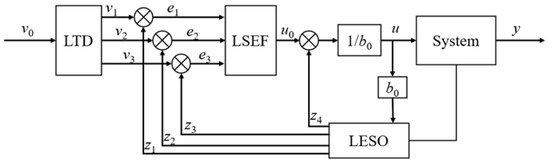
Figure 6.
Structural diagram of third-order linear automatic disturbance rejection controller.
3.1. Linear Tracking-Differentiator
As the transition process of the ADRC device, TD is mainly used to smooth the reference signal and generate its derivative signal for forming a smooth setpoint track and reducing the overshoot used by the step. For a third-order system, a multi-stage TD was designed, and its output is expressed as follows:
where is the input signal, is the smoothed reference signal, and are approximate differential signals of ; , , and are parameters adjusted according to the required transition performance.
Based on , and are substituted with , and the equation is obtained through Laplace transformation as follows:
The pole placement method can be used for the characteristic equation of the transfer function as follows:
The LTD parameter meets: , where v0 is the bandwidth of LTD, greater than zero, to obtain the transfer function as follows:
is taken as an input signal, where the amplitude is 0.2 m, time t is in seconds [s], and rad/s, to verify the effectiveness of the linear differential tracker design. Figure 7 shows the designed linear differential tracker model. The simulation results are shown in Figure 8.
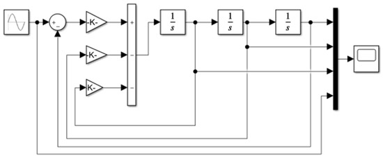
Figure 7.
The designed linear Tracking-Differentiator model.
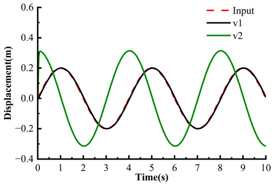
Figure 8.
Simulation results of linear tracking derivative.
The input signal curve extracted the input signal, and the difference curve is shown in Figure 8. The tracking signal quickly and accurately tracks the input signal v0, and LTD can also extract the differential signal of the input signal, though it is not accurate.
3.2. Linear Extended State Observer
The disturbance is considered an extended state to compensate for unmodeled uncertainties in the system. By defining system state variables and considering system modeling error and external interference, the transfer function of the electro-hydraulic position servo system can be converted into an extended state equation as follows:
where x1, x2, and x3 are the system state variables, x4 is the extended state variable, b0 is the compensation factor of the controller, y is the system output, and u is the system control input. f (x, u, d) includes both internal and external disturbances. The linear posting-state observer demonstrates good disturbance estimation and standardization effect on the nonlinear system. Considering controller realizability in engineering practice and the difficulty of parameter setting, this study adopted the LESO based on the bandwidth parameter setting of the observer.
The expansion state variable of the electro-hydraulic servo system can transform the following state-space equations:
In the equation,
LESO can be used to estimate the state and total interference of the system:
In the equation, is the gain matrix of the LESO, L0 satisfies the approximation and its order derivatives, and is the approximate total disturbance. The selection of parameter is usually carried out using the pole configuration method. If all poles of the observer are expected to be placed at , the characteristic polynomial of the fourth-order observer is expected to be:
Therefore, can be taken directly. The expansion state equation of LESO is
A simulation was conducted to verify the validity of the designed four-order LESO. Similarly, rad/s, with as the input signal, time t in [s], the electro-hydraulic servo system model used in this section was obtained using the system identification method, and the selected control object is
Here, G(s) denotes the spool–piston transfer function, representing the dynamic relationship between the valve spool displacement and the hydraulic cylinder piston displacement. Since both the input and output variables are in meters [m], the numerator constant “82.14” is dimensionless. It should be noted that this identified model is an approximate dynamic representation, which is used to replace the AMESIM co-simulation model during controller verification in MATLAB R2020b to simplify the analysis process.
Figure 9 shows the designed linear extended state observer model. The simulation results are shown in Figure 10. This design enables the observer to converge at a fast speed to accurately track the system state and disturbance.
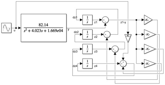
Figure 9.
The designed linear extended state observer model.
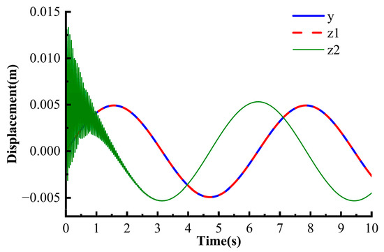
Figure 10.
Simulation results of linear extended state observer.
3.3. Linear State Error Feedback
The error was calculated according to TD outputs v1, v2, and v3 and LESO estimates z1, z2, and z3, and the control quantity was designed as follows:
In the equation, m1, m2, and m3 are the controller parameters. Total disturbance estimator z4(t) was used to compensate for system disturbance, and then the system was converted into an integrator series system. The final control signal is expressed as follows:
From Equations (12), (15), and (19)–(22), the following equations can be obtained by means of Laplace transformation:
The pole placement method meets the characteristic equation:
In the characteristic equation, the controller parameters meet . is the controller bandwidth, and the transfer equation is expressed as follows:
In summary, the combination of third-order LADRC algorithms is
Only four parameters, , , and , are required for the designed third-order linear automatic disturbance rejection controller.
4. Parameter Setting of Third-Order Linear Automatic Disturbance Rejection Controller
4.1. Determination of Compensation Factor b0
In the electro-hydraulic servo system, the variable x represents the output displacement of the hydraulic cylinder, while the state vector is introduced only for state-space modeling.
Therefore, the expression represents the acceleration of the output displacement, rather than the second derivative of the state vector.
Here, f is the total disturbance, and b0u is the effective acceleration generated by the control input.
To avoid ambiguity, we explicitly relate the state coordinates to the physical variables appearing in Equations (1)–(3). We define:
where is the piston displacement, is the piston velocity, is the load pressure, and denotes the total disturbance/uncertain term that acts on the acceleration equation.
It was assumed that the valve command u is proportional to the valve opening xv, i.e., xv = κu u, setting κu = 1 for simplicity, from which the following relations are obtained. Substituting this relation into the valve flow equation gives .
To clarify the modeling relationships, it should be noted that the physical model can be expressed as:
Equation (27) describes the ideal dynamic behavior derived directly from the force balance relationship of the hydraulic cylinder, without accounting for external disturbances or model uncertainties.
Therefore, we define the nominal model function as:
where denotes the state vector representing the piston displacement, velocity, and load pressure, respectively. It should be noted that in the overall state-space formulation, the extended state vector is defined as , x4 represents the total disturbance and unmodeled dynamics introduced in the extended state observer. The nominal model here only involves the first three physical states.
However, in the real system, unmodeled dynamics and external disturbances exist. Therefore, the actual acceleration can be expressed as:
where represents the estimated model term corresponding to , denotes the disturbance and unmodeled dynamics, and is the control input term in the LADRC formulation.
In this sense, corresponds to the ideal nominal model, while is the extended model used in LADRC design that accounts for both the control input and disturbance. The relationship between them can be summarized as: .
When the pressure dynamic bandwidth is much faster than the mechanical dynamic bandwidth, , from which can be derived. Substituting this into Equation (27) yields: .
The parameter b0 represents the equivalent gain from the control input u to the acceleration of the actuator. This can be derived as .
4.2. Hyperbolic Sine-Cosine Optimization
4.2.1. Selection Basis of Bandwidth Factor
First, it is necessary to specify the nominal bandwidth of the system. The approximate system characteristic frequency can be obtained through open-loop frequency domain simulation of the electro-hydraulic servo system. On this basis, the controller bandwidth and the observer bandwidth are defined as follows:
where and are referred to as bandwidth scaling factors. The offline search intervals for bandwidth scaling factors were set as [0.6, 1.8] and [1.8, 9] to ensure that the closed-loop system neither introduced excessive oscillations nor weakened the response speed.
The lower limit of 0.6 of this interval corresponded to a closed-loop bandwidth of about 0.6 to ensure that the response has the basic tracking capability; the upper limit of 1.8 corresponded to a closed-loop bandwidth of about 1.8 , providing a fast response with acceptable phase margin. Based on the empirical interval above, SCHO [22] can efficiently find the global near-optimal solution within the range of [0.6, 1.8] and [1.8, 9], thus avoiding the uncertainty caused by manual trial.
4.2.2. Construction of Multi-Objective Loss Function
To comprehensively reflect the impact of different on system performance, a weighted multi-objective loss function was introduced, where the first term is the integration data pair error, which is used to measure the average tracking deviation of the system in the time domain; the second term is the maximum overshoot, which is used to evaluate the peak overshoot amplitude in the system step response process and describe the dynamic stability; the third term is the control jitter term. The high-frequency jitter of the actuator is measured by the accumulated value of the change increment of the control quantity, and the hardware life can be extended by inhibiting excessive oscillation.
Specifically, the loss function is defined as
where is the maximum value of the desired displacement; is the maximum rate of change of the input signal. Therefore, all terms are dimensionless quantities.
The initial values of weights were , , and , which can achieve a good balance among tracking accuracy, dynamic stability, and control smoothness.
4.2.3. SCHO Principle
SCHO is a novel meta-heuristic algorithm [23]. Its core lies in realizing the global exploration of randomization and the local development of accuracy through different numerical characteristics of hyperbolic sine and cosine functions and enhancing convergence accuracy through a dynamic boundary reconstruction mechanism. Before being substituted into the hyperbolic sine and cosine functions, all position variables are normalized to the range [0, 1] according to their upper and lower bounds. This ensures that the arguments of sinh and cosh are dimensionless, thus maintaining the mathematical validity and numerical stability of the SCHO algorithm. The principle is explained in detail in three stages.
- Global exploration stage:
At the beginning of the iteration, SCHO uses the exponential growth characteristics of the sinh function to increase the search jump step, making the candidate solution cover a wide range of feasible domains as soon as possible. For example, for the ith individual (two-dimensional vector), if there is a large gap between its current position and the global optimum, the gap can be quickly amplified by multiplying the sinh function to make the individual jump out of the local extreme value. The updated formula is written as follows:
where is the random disturbance factor, which ensures diversity and avoids path fixation. In this case of , the sinh value increases rapidly and allows the candidate solution to jump out of the trap on a large scale.
- 2
- Local development stage:
When the population gradually converges to the promising region after several generations of iterations, the refined search for the region is required to further approach the global optimal solution. By virtue of the approximate linear and asymptotic convergence characteristics of the cosh function at small amplitude , SCHO makes the step size gentler and less likely to go beyond the boundary in later iterations. For the top performers (typically the top 20–30%), the updated formula is expressed as follows, including :
when the difference value is , is good for fine adjustments and accelerates the convergence of the solution in the later stage.
- 3
- Boundary reconstruction mechanism:
SCHO designed the triggered boundary contraction strategy to avoid an invalid search caused by the large-scale jump in the middle and late periods [24]. When the iteration number t meets the specific triggering conditions, the algorithm takes the current global optimum as the center, defines a new contraction radius , and updates the search space to the following:
where is the initial disturbance and is the contraction factor. At this point, if all individuals exceed the new boundary, they are projected back to this range so that the search is focused on the most promising region at present, further improving the convergence accuracy [25].
Through the organic combination of the above three stages, SCHO can not only explore the global region in the early stage but also gradually converge to the global optimal vicinity in the later stage and continuously reduce the search interval via dynamic boundary reconstruction to obtain a high-quality optimal solution.
4.3. Design of Fuzzy Controller
After completing offline global optimization to obtain the optimal factors and , the system enters the online control stage. At this time, taking and as the benchmark, the tracking error and its change rate are collected in real-time and input into the fuzzy inference module to make small adaptive corrections to the bandwidth factors of the LESO (Linear Extended State Observer) and the error feedback control law. In this way, under on-site disturbances such as servo valve parameter drift, sudden load changes, or measurement noise, the static limitations of offline optimization can be quickly compensated, maintaining the system’s tracking accuracy and dynamic performance.
Specifically, at every sampling period , the controller reads the reference signal and the measurement output , respectively, and calculates the instant error:
Its finite difference approximate derivatives are also calculated:
To eliminate the influence of different steel beams and amplitudes on the input of the fuzzy system, these two terms must also be quantified into a unified normalized interval as follows:
where and represent the “maximum expected error” and “maximum error rate of change”, respectively. Through this normalization process, and of the input fuzzy thruster are mapped to [0, 1], which not only makes the membership function design more universal, but also avoids the controller imbalance caused by dimensional difference and ensures that the fine adjustment of the bandwidth factor by the subsequent fuzzy rules is smooth and accurate.
The normalized approximate error eigenvalues and the introduction of seven membership sets, i.e., NB, NM, NS, ZO, PS, PM, and PB, were constructed, and the 7 × 7 rule matrix shown in Table 1 was constructed.

Table 1.
Fuzzy control rule table.
Fuzzy Rule: If belongs to and belongs to , belongs to and belongs to .
represents one of the seven official books, respectively.
Take the current input and calculate each of the five membership function values to obtain the following:
For the rule in line i, column j, define its activation as the minimum value of the two input membership:
For the two outputs of bandwidth adjustment and , the output membership functions corresponding to the rules are superimposed, respectively. Taking as an example, if the output membership function recommended by rule is , the following can be obtained after aggregation:
where represents the minimum value, and max represents the aggregation of the maximum values of the output membership of each rule.
The aggregated membership functions are converted into specific values via the center of gravity method as follows:
where and are the minimum and maximum values of bandwidth adjustment, respectively.
Based on the and values obtained via offline SCHO global optimization and the real-time fine-tuning mechanism of online fuzzy logic, a two-layer control strategy of “static global optimization first → dynamic local adaption” is formed. This strategy combines the robustness guarantee in global optimization and the working condition adaptability in online regulation so that the electro-hydraulic servo system can not only maintain fast and accurate tracking but also effectively suppress the noise amplification and execution vibration when facing a complex environment with an uncertain model and frequent disturbance, thereby significantly improving the overall control performance.
5. Simulation Analysis
To verify the performance of the proposed control strategy in practical nonlinear systems, this paper used AMESIM to establish a high-precision hydraulic system model and implemented the LADRC algorithm via Simulink for co-simulation. Based on actual working conditions, AMESIM is responsible for simulating the nonlinear dynamics of the valve-controlled cylinder, as shown in Figure 11. Partial parameters of the simulation are listed in Table 2. Simulink is responsible for the real-time calculation of the controller, as shown in Figure 12, to reflect the integration of theory and practice.

Figure 11.
Hydraulic system simulation.
Table 2.
Some parameters of servo valve control system.
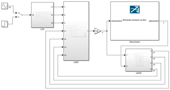
Figure 12.
LADRC algorithm design.
The system transmits the displacement speed signal of the hydraulic cylinder to MATLAB through the interface module and controls the servo valve opening through the output signal in MATLAB to control the hydraulic cylinder position. Similar interface modules are also required in Simulink to connect the two software to realize signal intercommunication. In this simulation, it was set so that the hydraulic cylinder started to move from the middle and control PID and LADRC, respectively.
A step signal with an amplitude of 0.5 was input to the control system. Figure 13 and Figure 14 show the response signal without and with an interference signal, respectively.
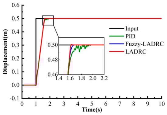
Figure 13.
Step response.
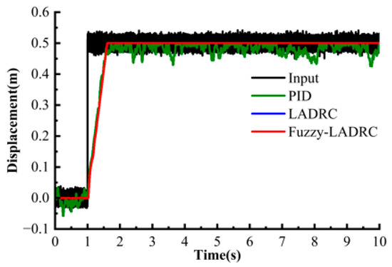
Figure 14.
Disturbance-added step response.
By comparing Figure 13 and Figure 14, the anti-disturbance performance of LADRC and Fuzzy-LADRC can be clearly verified. In a disturbance-free environment, PID showed obvious fluctuations, and the fluctuation range of its displacement peak and valley was significantly larger than that of LADRC and Fuzzy-LADRC. When a high-frequency disturbance was introduced, PID performance deteriorated sharply, and its displacement response exhibited intense oscillations and obvious lag throughout the transient phase of the entire step response, and the overall lagged the sine reference signal. In contrast, the displacement fluctuation range of LADRC was reduced to 0.019 m–0.020 m, and the oscillation amplitude was about 33% lower than that of PID. While Fuzzy-LADRC proved its excellent anti-disturbance ability with a trajectory almost coinciding with the reference signal, especially at the turning points of peaks/valleys, such as around t = 1.0 s, it could accurately track without lag, verifying that the LADRC framework effectively suppresses the influence of disturbances through the disturbance observer.
For the sinusoidal signal of input to the control system, where the amplitude was 0.2 m, and time t in seconds [s]. Figure 15 and Figure 16 shows the response signal without and with an interference signal, respectively.
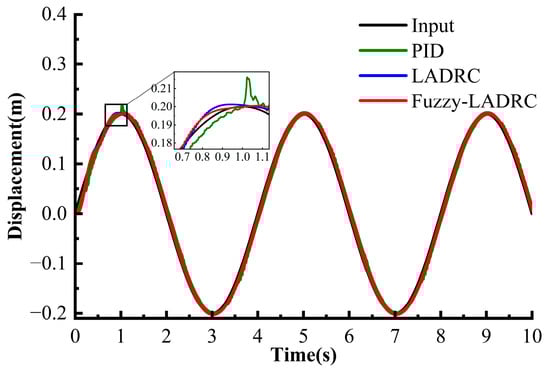
Figure 15.
Sinusoidal response.
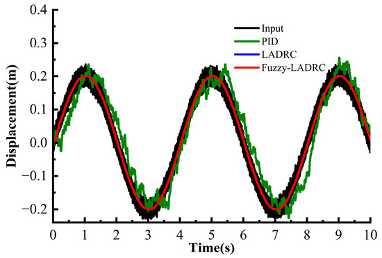
Figure 16.
Disturbance-added step response.
A combined analysis of Figure 15 and Figure 16 shows that Fuzzy-LADRC comprehensively upgrades its control performance based on LADRC. During the system disturbance phase, PID produced severe overshoot and exhibited continuous oscillation. Although LADRC reduced the overshoot, its stabilization time remained long. The partial enlargement in Figure 15 further revealed key differences: the PID response oscillated markedly around the target value, while the LADRC response showed reduced but still visible fluctuations without full convergence. In contrast, the Fuzzy-LADRC curve demonstrated superior performance, with a significantly smaller overshoot and a much faster convergence rate than both PID and LADRC. This indicates that the adaptive parameter adjustment mechanism of fuzzy logic effectively enhances the controller’s robustness under dynamic disturbances, enabling Fuzzy-LADRC to retain the anti-disturbance advantages of LADRC while achieving a faster transient response capability.
To study the influence of damping characteristics on the dynamic performance of the system, the damping coefficient in the shock absorber model was used as an adjustable variable, and a set of step responses with different damping coefficients as constructed and compared. By comparing the response curves in Figure 17 and Figure 18 under step input, the following conclusions can be drawn: the overshoot of PID control reached 33%, when the damping coefficient was 1000 N·s/m, while Fuzzy-LADRC reduced the overshoot to less than 5% under the same damping coefficient. In the working condition with a damping coefficient of 3000 N·s/m, the settling time of Fuzzy-LADRC was shortened by 40%. As the damping coefficient increased, the response speed of PID decreased by 30%, while the dynamic characteristics of Fuzzy-LADRC remained basically unchanged. The maximum displacement deviation of Fuzzy-LADRC under different damping coefficients was less than 0.02 m, while that of PID reached 0.05 m.
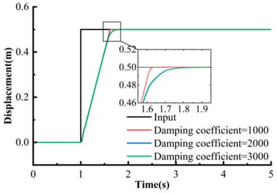
Figure 17.
Step response under PID control.
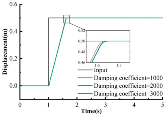
Figure 18.
Step response under Fuzzy-LADRC control.
Fuzzy-LADRC control significantly optimized the step response performance compared with PID: at the same damping coefficient, the overshoot was reduced from 33% to a negligible level, and the settling time was shortened by 40%; moreover, the dynamic robustness was improved—when the damping coefficient was perturbed, the displacement deviation was reduced from 0.05 m to 0.02 m, verifying its strong adaptability to parameter changes.
A set of sinusoidal responses under different damping coefficients was constructed and compared to study the influence of damping characteristics on the dynamic performance of the system in practical applications. By comparing the tracking curves in Figure 19 and Figure 20 under sinusoidal input, the following results were observed: under a sine wave, the phase lag of PID reached 25%, while Fuzzy-LADRC reduced the lag to less than 5%. The tracking amplitude of PID attenuated by 12%, while the amplitude error of Fuzzy-LADRC was less than 2%. PID showed harmonic distortion in the high-frequency band, whereas Fuzzy-LADRC maintained perfect sinusoidal characteristics. At a damping coefficient of 2000 N·s/m, the peak-to-peak value of PID output was 0.24 m, while Fuzzy-LADRC reduced it to 0.10 m.
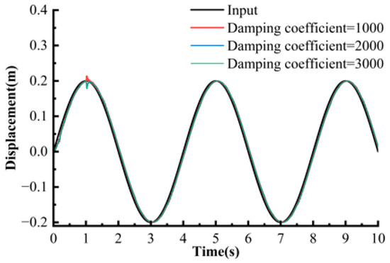
Figure 19.
Sinusoidal response under PID control.
Figure 20.
Sinusoidal response under Fuzzy-LADRC control.
When the damping coefficient increased to 3000 N·s/m, the PID curve still had a jitter of ±0.05 m, while the fluctuation amplitude of Fuzzy-LADRC was less than 0.01 m. Fuzzy-LADRC achieved breakthrough improvements in sinusoidal tracking: compared with the phase lag and amplitude attenuation of PID, its phase lag was compressed to within 0.05 s, the amplitude error was <2%, and high-frequency harmonic distortion was eliminated. The anti-disturbance capability was simultaneously enhanced, with the fluctuation amplitude reduced by 58% at a damping coefficient of 2000 N·s/m.
Testing under variable disturbances is crucial for verifying the robustness of the controller. A new simulation was conducted to address the more complex and time-varying interference in system applications. The signal given is:
and .
The comparative analysis of displacement response of the system under different signals is shown in Figure 21 and Figure 22. It can be clearly seen that the Fuzzy LADRC controller performed better than the PID controller in managing the transition process. Specifically, the oscillation in the Fuzzy LADRC response was significantly suppressed, and the system could reach the steady state faster and smoother, which confirms its enhanced robustness and control accuracy.
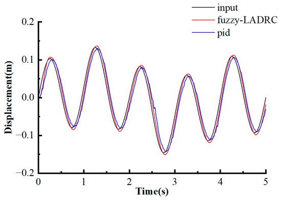
Figure 21.
Response under y1 signal.
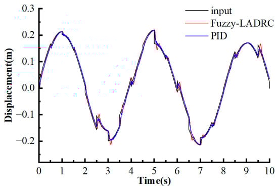
Figure 22.
Response under y2 signal.
Four curves were obtained to explore the dynamic response characteristics of the system under a fixed damping coefficient, as shown in Figure 23. The simulation results showed good system dynamic and linear damping characteristics: the displacement curve (Figure 23a) was a smooth sine wave with an amplitude of ±0.2 m, indicating that the hydraulic system has high tracking accuracy for periodic excitation; the velocity curve (Figure 23b) as differentially related to the displacement (phase lead: 90°; peak value: ±0.4 m/s), verifying the excitation signal quality; the force curve (Figure 23c) fluctuated in the same phase with the velocity (peak value ±2000 N), reflecting the dynamic response of the linear damping force. The closed hysteresis loop (Figure 23d) indicates that the actuator dissipates energy in each cycle; the area of the hysteresis loop corresponds to the energy dissipated during each cycle. Specifically, the compressibility of oil can generate a quasi-elastic energy storage effect and cause pressure to lag piston displacement. Nonlinear valve flow and internal and external leakage will introduce additional phase lag and energy dissipation. The overall results consistently reflect the stable dynamic process of the hydraulic system driving the linear damping element, and the data had no significant transient interference, providing a reliable basis for subsequent model verification and control algorithm optimization.


Figure 23.
Dynamic response characteristics of the shock absorber with fixed damping coefficient.
6. Conclusions
In this study, detailed mathematical models of the servo valve control cylinder and the hydraulic shock absorber were established, respectively. The input–output relationship of the system was derived from the valve port flow, the oil cavity dynamics, and the actuator characteristics of the valve core. The dynamic equations of longitudinal vibration were established for the latter by combining the elastic and damping forces. On this basis, a third-order linear automatic disturbance rejection controller was designed, which realized the online estimation and compensation of unknown disturbances to the system through three modules: tracking derivative, linear extended state observer, and linear error feedback law. Then, hyperbolic sine-cosine optimization (SCHO) was used for the global optimization of key LADRC parameters to ensure that the control performance could reach the optimal compromise among multiple targets (such as overshoot, steady-state error, and response time), and the fuzzy control principle was introduced to perform real-time adaptive regulation on partial feedback gain to account for fast response and overshoot suppression. The simulation and experiment results show that the composite control strategy not only significantly improves the dynamic response speed and robustness of the system, but also shows excellent anti-interference ability and a vibration reduction effect under complex working conditions.
Author Contributions
Conceptualization, M.Z., Z.C. and X.H.; methodology, M.Z., Z.C. and X.H.; software, Z.C. and X.H.; validation, Z.C. and X.H.; formal analysis, M.Z., Z.C. and X.H.; investigation, M.Z.; resources, M.Z.; data curation, Z.C., X.H. and X.Z.; writing—original draft preparation, M.Z., Z.C. and X.H.; writing—review and editing, M.Z., Z.C. and C.X.; visualization, M.Z.; supervision, M.Z.; project administration, M.Z.; funding acquisition, M.Z. All authors have read and agreed to the published version of the manuscript.
Funding
This research was funded by the National Natural Science Foundation of China Youth Fund Projects (52405062 and 52405063).
Data Availability Statement
Data is contained within the article.
Conflicts of Interest
Author Chao Xun was employed by the company Ningbo Jingqiong Machinery Manufacturing Co., Ltd. The remaining authors declare that the research was conducted in the absence of any commercial or financial relationships that could be construed as a potential conflict of interest.
References
- Cao, X.; Zhao, Z.; Zhu, W.; Lian, G.; Ye, M.; Alam, M.M. Ride comfort analysis of hydro-pneumatic suspension considering variable damping matched with dynamitic load. Int. J. Hydromechatron. 2025, 8, 317–342. [Google Scholar] [CrossRef]
- Hu, J.; Qiang, H.; Liu, K.; Kang, S.; Yang, J.; Wang, L. Research on load displacement tracking control of hydraulic damper test bench based on sliding mode active disturbance rejection control. Mach. Tool Hydraul. 2025, 53, 73–80. [Google Scholar] [CrossRef]
- Righettini, P.; Strada, R.; Tiboni, M.; Cortinovis, F.; Santinelli, J. A systematic management and control methodology for high energy saving in applications equipped with hydraulic servo-axes. Control Eng. Pract. 2024, 146, 105847. [Google Scholar] [CrossRef]
- Ling, Q.; Chen, X.; Niu, L.; Guo, Y.; Chen, S. Performance evaluation and analysis for hydraulic active suspension using the collaborative control method. Meas. Control 2025, 58, 771–783. [Google Scholar] [CrossRef]
- Ji, X.; Wang, C.; Zhang, Z.; Chen, S.; Guo, X. Nonlinear adaptive position control of hydraulic servo system based on sliding mode back-stepping design method. Proc. Inst. Mech. Eng. Part I J. Syst. Control Eng. 2021, 235, 474–485. [Google Scholar] [CrossRef]
- Kan, K.; Yu, Y.; Chen, Y.; Qiao, P.; Ye, C.; Binama, M. Multi-scale flow-induced dynamic response in 710-MW Francis turbine: Numerical investigation. Int. J. Mech. Sci. 2025, 296, 110345. [Google Scholar] [CrossRef]
- Sharifi, S.; Tivay, A.; Rezaei, S.M.; Zareinejad, M.; Mollaei-Dariani, B. Leakage fault detection in electro-hydraulic servo systems using a nonlinear representation learning approach. ISA Trans. 2018, 73, 154–164. [Google Scholar] [CrossRef] [PubMed]
- Liu, F.; Yang, Y.; Wang, L. Active Disturbance Rejection Control Design for the Hydraulic Actuator on Weeding Machine. In Proceedings of the 2021 40th Chinese Control Conference (CCC), Shanghai, China, 26–28 July 2021. [Google Scholar] [CrossRef]
- Jin, K.; Song, J.; Li, Y.; Zhang, Z.; Zhou, H.; Chang, X. Linear active disturbance rejection control for the electro-hydraulic position servo system. Sci. Prog. 2021, 104, 00368504211000907. [Google Scholar] [CrossRef]
- Hanaffi, M.S.; Ghani, M.F.; Jaafar, H.I.; Soon, C.C. Improved PID controller for an electro-hydraulic system using particle swarm optimization. In Proceedings of the 2023 IEEE 21st Student Conference on Research and Development, Kuala Lumpur, Malaysia, 13–14 December 2023; pp. 533–538. [Google Scholar] [CrossRef]
- Essa, M.E.-S.M.; Aboelela, M.A.; Hassan, M.M.; Abdrabbo, S. Design of model predictive force control for hydraulic servo system based on cuckoo search and genetic algorithms. Proc. Inst. Mech. Eng. Part I J. Syst. Control Eng. 2019, 234, 701–714. [Google Scholar] [CrossRef]
- Essa, M.E.-S.M.; Aboelela, M.A.S.; Hassan, M.M.; Abdrabbo, S.M. Model predictive force control of hardware implementation for electro-hydraulic servo system. Proc. Inst. Mech. Eng. Part C J. Mech. Eng. Sci. 2019, 233, 1435–1446. [Google Scholar] [CrossRef]
- Naveen, C.; Meenakshipriya, B.; Thomas, A.T.; Sathiyavathi, S.; Sathishbabu, S. Real-time implementation of iterative learning control for an electro-hydraulic servo system. IETE J. Res. 2022, 69, 649–664. [Google Scholar] [CrossRef]
- Hoang, Q.-D.; Lee, S.-G.; Dugarjav, B. Super-twisting observer-based integral sliding mode control for tracking the rapid acceleration of a piston in a hybrid electro-hydraulic and pneumatic system. Asian J. Control 2019, 21, 483–498. [Google Scholar] [CrossRef]
- Ren, J.; Chen, Z.Q.; Yang, Y.K.; Sun, M.W.; Sun, Q.L.; Wang, Z.H. Grey Wolf Optimization Based Active Disturbance Rejection Control Parameter Tuning for Ship Course. Int. J. Control Autom. Syst. 2022, 20, 842–856. [Google Scholar] [CrossRef]
- Xiao, L.; Liu, W.; Zhu, X.; Tan, Y. Intelligent sliding mode tracking control for electro-hydraulic position servo systems based on variable exponential power reaching law with CGWO-PSO. Trans. Inst. Meas. Control 2024, 47, 2139–2151. [Google Scholar] [CrossRef]
- Ji, X.W.; He, X.K.; Lv, C.; Liu, Y.H.; Wu, J. A vehicle stability control strategy with adaptive neural network sliding mode theory based on system uncertainty approximation. Veh. Syst. Dyn. 2018, 56, 923–946. [Google Scholar] [CrossRef]
- Liu, C.; Luo, G.; Chen, Z.; Tu, W.; Qiu, C. A linear ADRC-based robust high-dynamic double-loop servo system for aircraft electro-mechanical actuators. Chin. J. Aeronaut. 2019, 32, 2174–2187. [Google Scholar] [CrossRef]
- Wang, Z.G.; Yu, C.Y.; Li, M.J.; Yao, B.H.; Lian, L. Vertical Profile Diving and Floating Motion Control of the Underwater Glider Based on Fuzzy Adaptive LADRC Algorithm. J. Mar. Sci. Eng. 2021, 9, 698. [Google Scholar] [CrossRef]
- Bao, H.; He, D.; Zhang, B.; Zhong, Q.; Hong, H.; Yang, H. Research on Dynamic Performance of Independent Metering Valves Controlling Concrete-Placing Booms Based on Fuzzy-LADRC Controller. Actuators 2023, 12, 139. [Google Scholar] [CrossRef]
- Zhang, F.; Hou, J.; Ning, D.; Gong, Y. Depth Control of an Oil Bladder Type Deep-Sea AUV Based on Fuzzy Adaptive Linear Active Disturbance Rejection Control. Machines 2022, 10, 163. [Google Scholar] [CrossRef]
- Bai, J.; Li, Y.; Zheng, M.; Khatir, S.; Benaissa, B.; Abualigah, L.; Abdel Wahab, M. A Sinh Cosh optimizer. Knowl.-Based Syst. 2023, 282, 1.1–1.29. [Google Scholar] [CrossRef]
- Ekinci, S.; Izci, D.; Gider, V.; Abualigah, L.; Bajaj, M.; Zaitsev, I. Optimized FOPID controller for steam condenser system in power plants using the sinh-cosh optimizer. Sci. Rep. 2025, 15, 6876. [Google Scholar] [CrossRef] [PubMed]
- Jiang, S.; Cui, S.; Song, H.; Lu, Y.; Zhang, Y. Enhanced Nutcracker Optimization Algorithm with Hyperbolic Sine–Cosine Improvement for UAV Path Planning. Biomimetics 2024, 9, 757. [Google Scholar] [CrossRef] [PubMed]
- Izci, D.; Rizk-Allah, R.M.; Snášel, V.; Ekinci, S.; Migdady, H.; Daoud, M.S.; Altalhi, M.; Abualigah, L. Refined sinh cosh optimizer tuned controller design for enhanced stability of automatic voltage regulation. Electr. Eng. 2024, 106, 6003–6016. [Google Scholar] [CrossRef]


Disclaimer/Publisher’s Note: The statements, opinions and data contained in all publications are solely those of the individual author(s) and contributor(s) and not of MDPI and/or the editor(s). MDPI and/or the editor(s) disclaim responsibility for any injury to people or property resulting from any ideas, methods, instructions or products referred to in the content. |
© 2025 by the authors. Licensee MDPI, Basel, Switzerland. This article is an open access article distributed under the terms and conditions of the Creative Commons Attribution (CC BY) license (https://creativecommons.org/licenses/by/4.0/).