Abstract
The blade is a core component of the gas turbine, and blade fouling is characterized by highly concealed failure modes in the early stages and significant destructive potential in later stages. To address the lack of intelligence in early warning systems for compressor fouling, this study proposes a data-driven approach combining a digital-twin-based dynamic simulation model with the Weibull Proportional Hazards Model (WPHM) algorithm to enable reliable fault early warning. A modular design methodology was first adopted to construct a digital gas turbine model of the gas–gas combined power system on a dynamic simulation platform. High-fidelity fault simulation data were then generated to represent both healthy and faulty operating conditions. Through data governance and uncertainty quantification, key parameters influencing compressor fouling were identified. The Pearson correlation coefficient was applied to screen the most sensitive indicators, ensuring effective input selection for the prognostic model. Using historical health data from the simulation platform, the WPHM algorithm was trained to learn degradation patterns and establish a baseline failure risk model. This trained WPHM was then deployed to monitor real-time performance trends and provide early warnings for compressor blade fouling. Validation results from multi-unit simulations show that the proposed method achieves a fault warning rate of 95.0%, demonstrating its effectiveness and readiness to meet practical engineering requirements.
1. Introduction
Fouling of compressor blades is one of the typical faults in marine gas turbines. It poses hazards throughout the entire operation cycle of the gas turbine [1,2]. On one hand, fouling alters the aerodynamic shape of the blade surface. This increases airflow resistance. As a result, the compressor pressure ratio and flow rate decrease. The overall output power of the gas turbine is therefore reduced. At the same time, fuel consumption increases. These changes reduce the operational efficiency of the power system [3]. On the other hand, performance degradation caused by fouling intensifies fatigue damage to the blades. This shortens the service life of components. Troubleshooting and cleaning require disassembly of the power system. This increases maintenance workload and costs [4]. It also extends the ship’s out-of-service time. Marine gas turbines operate in a special environment. During navigation, salt in the air, marine biological residues, and atmospheric particles can all contribute to fouling [5]. When the compressor runs at high speed, blades endure alternating aerodynamic and mechanical loads. Uneven fouling distribution further worsens load fluctuations. This creates a vicious cycle: “fouling → load deterioration → accelerated damage.” Compressor fouling has thus become a key factor affecting the reliability of marine power systems [6].
Scholars worldwide have conducted extensive research on the mechanism and impact of compressor fouling. Yang and Cai [7] carried out experimental studies on blade contamination. They found that, at the same rotational speed, increased contamination leads to a drop in both pressure ratio and efficiency. Higher rotational speeds result in a stronger inhibitory effect on flow rate. The inlet pressure difference is the most sensitive parameter reflecting fouling degree. This provides an important basis for selecting fault characteristic parameters. From the perspective of fault chain reactions, Liu, et al. [8] pointed out that long-term untreated fouling causes a continuous drop in intake flow and an abnormal rise in inlet temperature. Once airflow stability is lost, surge faults are easily triggered. There is a clear correlation between different fouling levels and changes in characteristic parameters. This lays the foundation for quantitative fault analysis. Tarada and Suzuki [9] tested the surface roughness of 58 fouled compressor blades from aviation, marine, and industrial gas turbines. Results showed that fouling increases surface roughness. The distribution is uneven. A single uniform roughness parameter cannot fully describe its impact on aerodynamic performance. Further research by Bons, et al. [10] in marine environments revealed that salt and sand dust together accelerate fouling formation and hardening. Over time, some fouling may flake off due to airflow scouring. This leads to a dynamic change in surface roughness: “increase—local decrease.” This behavior provides valuable insights for modeling fault evolution in dynamic simulations. As gas turbine performance increasingly affects ship safety and operating costs, industry demands for power system reliability continue to rise [11,12].
With rapid advances in computer technology, sensors, and intelligent algorithms, fault diagnosis is now widely applied in gas turbines [13]. The United States established a special project group focused on health management of marine gas turbine propulsion systems [14,15,16]. By developing high-precision sensors, real-time diagnosis algorithms, and integrated control–diagnosis systems, they upgraded the health management system for the C-17T-1 transport aircraft [17]. This enabled early fault detection and trend prediction. Major industrial gas turbine manufacturers—GE (USA), Mitsubishi (Japan), and Siemens (Germany)—have also invested in condition monitoring and fault diagnosis for marine applications [18]. Optimized sensor layouts and improved data analysis have reduced downtime and enhanced operational economy and reliability [19]. In intelligent diagnosis, Botros, et al. [20] demonstrated that radial basis function neural networks perform well in fault monitoring when engine parameters are limited. They compared multi-layer perceptrons, radial basis functions, and regression networks. The results confirmed the superiority of radial basis networks under small-sample and high-noise conditions. HS Tan [21] applied Fourier neural networks and single-hidden-layer networks to fault classification. Real-world data tests achieved accurate fault identification. This opened a new path for engineering applications of intelligent diagnosis. Rajeev, et al. [22] combined a linearized gas turbine model with a radial basis function network. The neural network preprocessed fault data, reducing noise and improving fault separation robustness. This offers technical support for diagnosis under complex conditions. The Weibull Proportional Hazards Model (WPHM) adopted in this study is a semi-parametric regression model developed by British statisticians [23]. Renowned for its ability to capture a variety of failure modes and eliminate interference signals, this algorithm has since been widely applied in equipment condition prediction. Wang [24] proposed a KPCA-WPHM-based predictive method for bearing reliability assessment. Banjevic and Jardine. [25] integrated Markov stochastic processes with WPHM for transmission case reliability prediction. Although this algorithm has been extensively utilized in aviation propulsion system reliability analysis, there remains a notable gap in related research on marine combustion propulsion systems.
The development of numerical simulation technology offers a new way to dynamically analyze compressor fouling faults. Kang, et al. [26] used numerical simulation to study an important issue. They focused on how compressor blade surface roughness—a key indicator of fouling—affects the aerodynamic performance of cascades. Their results showed a clear trend: as blade surface roughness increases, airflow friction loss and separation loss rise. This leads to a sharp drop in cascade efficiency. Furthermore, this extra loss is the main cause of reduced compressor stage efficiency. It provides a theoretical basis for quantitatively simulating how fouling faults impact performance. Rowen [27,28] carried out a comparative study. He took experimental test data of a certain type of marine gas turbine compressor blade. He then compared it with finite element numerical simulation results. This comparison verified that numerical simulation is accurate in calculating blade natural frequency. He also performed further analysis. He explored how fouling-induced changes in blade mass distribution affect natural frequency. This work provides a method reference for simulating structural dynamic characteristic changes caused by faults. Camporeale, et al. [29] adopted a specific approach. They used transient thermodynamic analysis to numerically simulate the working process of compressor blades. Their findings were notable: fouling reduces heat dissipation performance. This reduction intensifies the blade temperature gradient. A steeper temperature gradient then increases thermal stress. Higher thermal stress accelerates blade creep damage. This research lays a foundation for multi-physics field coupling simulation of fouling faults.
However, current domestic and foreign research on gas turbine compressor fouling faults still has shortcomings. On one hand, most studies have a narrow focus. They concentrate on performance analysis or fault mechanism exploration of a single compressor component. They lack modular modeling of the entire gas–gas combined power system [30]. This makes it hard to fully show how fouling faults have a chain impact on the power system’s overall performance. On the other hand, existing studies have a delayed focus [31]. They mostly analyze performance degradation after faults occur. Few studies focus on dynamic simulation and early warning of the fault evolution process. This fails to meet the needs of marine power systems. Marine power systems require “early detection and early intervention” for faults. Given these challenges, this paper puts forward a solution. Marine gas turbine fault experiments have high costs, long cycles, and difficulty in reproducing extreme working conditions. So, this paper proposes to obtain fault data through digital simulation technology. It also suggests integrating dynamic simulation models with intelligent algorithms. The goal is to build a compressor fouling fault identification method [32,33].
Actual machine fault experiments have high costs and high risks. Considering this, this paper proposes a compressor fouling fault early warning method. It integrates a digital gas turbine dynamic simulation model with the Weibull Proportional Hazards Model (WPHM) algorithm. The method has several key steps. First, a high-precision component-level model is built. This is based on the gas turbine’s operation mechanism and actual operation data. Then, environmental noise disturbance is introduced. This step completes the dynamic calibration of the model. Next, general simulation modules are processed. They are coupled and connected. This helps establish an overall dynamic simulation platform. The platform is for the gas–gas combined power system. On this platform, a new module is designed. It is a fault injection module. Its design centers on a typical fouling degradation curve. This module is used to simulate a specific process: the compressor’s performance degradation under different working conditions. During simulation, multi-dimensional operation data is collected. The data covers both healthy and fault states of the compressor. Further work involves parameter screening. Data governance, uncertainty quantification, historical operation data, and expert experience are all used. The goal is to screen key characteristic parameters. These parameters are sensitive to fouling. With these parameters, an early warning WPHM is built. The model is for compressor fouling faults.
Finally, the model is put into use. First, the model is trained. It learns the boundary of normal compressor operation. Then, real-time monitoring is carried out. It tracks the evolution trend of deviations. The deviations are between the model’s predicted values and actual measured values. Based on this, the component failure rate is calculated. If the failure rate exceeds a preset threshold, the system acts automatically. It triggers an alarm. This realizes early identification and early warning of compressor fouling faults.
2. Modeling of Gas–Gas Power System
To accurately simulate the dynamic behavior of a gas–gas combined power system under real operating conditions, the modular modeling approach is adopted in MATLAB/Simulink R2021a, where general component modules are interconnected to form a complete system model. Special attention is given to ensuring seamless interface compatibility and reliable data transmission between modules, enabling accurate coupling of mass, energy, and control signals across components. To enhance the model’s fidelity and reliability, key physical parameters are carefully calibrated using actual engineering data and equipment specifications, including gas turbine combustion characteristics, gearbox transmission ratios, and controllable-pitch propeller thrust coefficients. This parameterization process ensures that the simulation closely reflects real-world system dynamics. Once the model is fully configured, the integrated gas–gas dynamic simulation platform is activated to replicate a wide range of operational scenarios and transient conditions, supporting subsequent fault simulation, performance analysis, and early warning algorithm development.
2.1. Gas Turbine Modeling
2.1.1. Compressor Module Modeling
The off-design condition study of the compressor is the key to ensuring the accuracy of the gas turbine model. The compressor characteristic curve queries the functional relationship between the corrected flow rate and isentropic efficiency with respect to the pressure ratio, corrected speed, and inlet guide vane angle [34].
where Gc is the mass flow rate of the compressor (unit: kg/s); Pin,c is the total inlet pressure of the compressor (unit: Pa); Tin,C is compressor inlet temperature (unit: K); n is rotational speed normalized by inlet temperature (unit: r/min); πC is compressor pressure ratio (dimensionless); ηC is compressor isentropic efficiency (dimensionless); f1 and f2 are characteristic functions; IGV represents the inlet guide vane angle. The corrected flow rate and efficiency can be obtained from the pressure ratio, corrected speed, and functional relationship. Only three of the five parameters need to be determined to completely determine the working state of the compressor.
Meanwhile, the outlet temperature of each sub-module of the compressor is:
where Tin,C, Tout,C are the inlet and outlet temperatures of the compressor; πC, ηC are the pressure ratio and efficiency of the compressor; kα is the specific heat ratio of air.
After determining the outlet temperature of each section, the power consumed by each sub-module of the compressor is:
where Gin,C is the inlet air flow rate of the compressor and Cpa is the specific heat capacity at constant pressure of air.
2.1.2. Combustion Chamber Module Modeling
The working process of the combustion chamber is to mix and burn the high-pressure air from the outlet of the compressor with fuel to become high-temperature gas for the turbine to work. Consider the volume inertia of the combustion chamber and ignore the thermal inertia. The key to modeling the combustion chamber is the change trend of the outlet temperature and the change of the pressure loss of the combustion chamber.
From the mass conservation equation and energy conservation equation:
where VB is the volume of the combustion chamber, ηB is the efficiency of the combustion chamber, Hu is the lower heating value of the fuel, and Gf is the fuel mass flow rate.
Substituting the ideal gas state equation of Equation (6) into the mass equation yields the combustion chamber pressure calculation equation of Equation (7), as follows:
where Pout,B is the outlet pressure of the combustion chamber; Tout,B is the outlet temperature of the combustion chamber; VB is the volume of the combustion chamber; Rg is the gas constant of the gas; Cpg,B is the specific heat of the gas at the outlet of the combustion chamber; ηB is the combustion efficiency of the combustion chamber; kg is the specific heat ratio of the gas; hin,B is the enthalpy of the inlet air of the combustion chamber; Hu is the lower heating value of the fuel; hout,B is the enthalpy value of the outlet gas of the combustion chamber; Gin,B is the inlet air flow rate of the combustion chamber; Gout,B is the mass flow rate of the outlet gas of the combustion chamber.
According to the mathematical model of the combustion chamber dynamic process in the formula, a constant specific heat combustion chamber simulation model can be established and encapsulated on the dynamic simulation platform, including two sub-modules: the heat exchange module and the volume module.
2.1.3. Turbine Module Modeling
The power turbine and high-pressure turbine are similar to the compressor module. The turbine characteristic curve provides the functional relationship between the corrected flow rate and adiabatic expansion efficiency with respect to the expansion ratio and corrected speed.
The outlet temperature of the turbine is:
where Tin,T and Tout,T are the inlet and outlet temperatures of the turbine; πT and ηT are the expansion ratio and efficiency of the turbine; Kg is the specific heat ratio of the gas.
After determining the outlet temperature of the turbine, the calculation formula for the turbine expansion work is:
where Gin,T is the inlet gas flow rate of the turbine and Cpg is the specific heat capacity at constant pressure of the gas.
2.1.4. Integration of Gas Turbine Dynamic Simulation Model
On the dynamic simulation platform, general simulation modules for packaged components are selected and interconnected to construct a single-rotor split-shaft gas turbine system simulation model, as illustrated in Figure 1. The simulation is conducted using MATLAB/Simulink R2021a, a widely adopted and well-established platform for modeling and simulating complex power systems, providing an environment for dynamic system analysis. The steady-state calculation is a step-by-step iteration method, and the dynamic calculation is a fully non-linear method. Then, set the initial parameters of each component to complete the construction of the gas turbine dynamic simulation model.
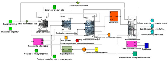
Figure 1.
Diagram of a dynamic simulation model of a gas turbine.
2.2. Modeling of Transmission and Propulsion Devices
2.2.1. Gearbox Modeling
The gearbox is a mechanical transmission device whose main function is to transmit power from one rotating shaft to another and realize the conversion of different speeds and torques. The gearbox is usually composed of a set of gears, each with different sizes and numbers of teeth. Through the meshing of gears, the gearbox can realize the increase or decrease in speed and torque.
Its mathematical formula can be expressed as:
where i = nc1/n1 = nc2/n1 refers to the gear ratio of the gearbox; ηg refers to its efficiency; Mc1 and Mc2 refer to the two input torques; M1 refers to the output torque; nc1 and nc2 refer to the two input speeds; n1 refers to the output speed.
2.2.2. Propeller Modeling
The propeller is a device that rotates in a fluid, and its main function is to generate thrust through rotational motion to drive the vehicle to move in the fluid. The power generated by the gas turbine is transmitted to the propeller, which is converted into thrust to push the ship forward. The thrust and torque of the propeller can be calculated by the following mathematical formulas:
where KT refers to the thrust coefficient of the propeller; ρ refers to the seawater density; np refers to the rotational speed; D refers to the diameter; KQ refers to the torque coefficient. The thrust coefficient and torque coefficient of the propeller can be obtained by checking the open water characteristic curve of the propeller through the advance coefficient, pitch ratio, and cavitation coefficient:
where σ refers to the cavitation coefficient; J refers to the advance coefficient of the propeller; P/D refers to the pitch ratio.
2.2.3. Integration of Dynamic Simulation Model of Gas–Gas Power System
According to the developed dynamic simulation models of key components such as gas turbines, gearboxes, and controllable pitch propellers, the modular design idea can be adopted to effectively integrate these models. As shown in Figure 2, in this way, the models of each component are no longer isolated but can be connected and work together to form a complete system simulation model. Simultaneously, in order to better demonstrate the dynamic simulation model of the power system, we show the design parameters and operational parameters in the model in Table 1.
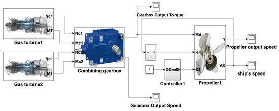
Figure 2.
Dynamic simulation model diagram of the combined dual-fuel power system.

Table 1.
Model parameter specification table.
By comparing the simulation data from the digital dynamic model of the gas turbine with literature data [34], as shown in Table 2, we observed that there were certain deviations between the performance indicators and reference values. This discrepancy stems from noise disturbances introduced during simulation. Although these deviations exist, they remain within a controlled error range of 5%. Based on comparative analysis with existing literature data, the reliability of the simulation model’s derived data is confirmed.
Table 2.
Simulation Platform Parameter Verification Table [34].
3. Compressor Fouling Fault Simulation
Compressor fouling fault is one of the main causes of gas turbine performance degradation, and its severity cannot be ignored. Blade fouling accounts for about 70–85% of the causes of gas turbine performance degradation. During the operation of the gas turbine, the air intake per kilowatt-hour of power is as high as 0.5 tons, and the tiny particles in the air, such as soot, oil mist, carbon particles, and sea salt, may pass through the filter and enter the machine despite the presence of the air filter. Over time, the accumulation of these particles on the blade surface will gradually form fouling, thus changing the blade geometry, inlet angle, and surface roughness, leading to a deterioration of the compressor aerodynamic performance. Fouling not only seriously affects the efficiency and reliability of the gas turbine but also may lead to an increase in maintenance costs and operating risks, thereby threatening the stability and safety of the entire power system. Therefore, timely identification and treatment of compressor fouling faults are crucial to ensure the long-term stable operation of the gas turbine.
Through an in-depth analysis of the mechanism of compressor fouling faults and based on the twin-shaft gas turbine simulation model developed by Lin Xinzhi, it is established that a 7% reduction in compressor flow rate and a 2% reduction in compressor efficiency are used as the threshold criteria for identifying the occurrence of fouling faults [35], as illustrated in Figure 3. To simulate the state and performance changes of the compressor when blade fouling occurs at a specific time, a fault module is introduced into the model, with a typical fouling evolution curve at its core. The fault module works by constructing a characteristic function that adheres to the predefined fault criteria for each component and allows setting the exact time of fault initiation based on research requirements. Once the fault is triggered, the function applies a time-varying perturbation to key parameters using a sine-based profile. Specifically, compressor fouling is simulated by perturbing the flow rate as 7% × sin(πt/T) and the efficiency as 2% × sin(πt/T), where T = 1000 s. This approach models the gradual accumulation of fouling, with the perturbation intensity starting at zero and increasing smoothly to its maximum over the course of 1000 s, effectively capturing the progressive nature of the fault.
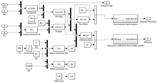
Figure 3.
Compressor fouling fault module.
Based on the established fault simulation method, a fault data generation process was developed for the gas–gas combined power system. The gas turbine in this study is a single-rotor split-shaft marine type, with its configuration, component parameters, and performance characteristics referencing the model detailed in [34]. To meet fault identification requirements, key monitoring parameters were selected, including the temperature, pressure, and rotational speed of relevant components—specifically covering the compressor outlet (flow rate, temperature, pressure), combustion chamber outlet (temperature, pressure), high-pressure turbine outlet (temperature, expansion ratio), and power turbine outlet (temperature, expansion ratio) at critical component interfaces. As illustrated in Figure 4, corresponding measurement points were deployed on the simulation platform to capture these parameters in real time, while the simulation was implemented in MATLAB/Simulink R2021a at a 1 Hz sampling frequency (1 sample per second); each of the 120 simulation units ran for 10,000 s, generating 10,000 data points per measurement channel per unit, which lays a foundation for fault detection algorithm development and performance evaluation.
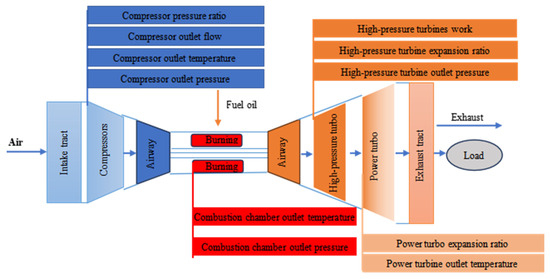
Figure 4.
Parametric measurement point distribution diagram.
After introducing compressor fouling faults into the simulation, performance fluctuations across all system components became evident, as shown in Figure 5. Parameters such as compressor flow rate, combustion chamber outlet temperature, power turbine expansion ratio, and high-pressure turbine outlet temperature exhibited a clear degradation trend, directly indicating that compressor fouling impairs overall system performance. Notably, the fault’s rapid manifestation (observable within minutes) is an accelerated simulation designed to meet engineering research needs—while actual compressor fouling develops gradually over months or even years, this accelerated approach (common in turbine fault studies [35]) effectively shortens the research cycle while preserving the fault’s essential progressive performance degradation characteristics. The validity of this simulation strategy was verified by comparing results with Lin Xinzhi et al.’s experimental data [35]: the simulated trends of flow rate and efficiency reduction aligned well with their long-term experimental observations, confirming the reliability and fidelity of the proposed simulation method. To meet the requirements for constructing and training subsequent fault prediction models, a total of 24 simulated compressor fouling units were established (each with different fault durations to verify model effectiveness across different units). Data collected from relevant measurement points will be used for subsequent fault analysis and identification.
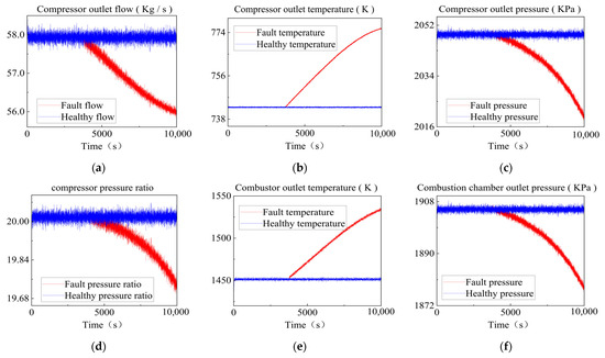
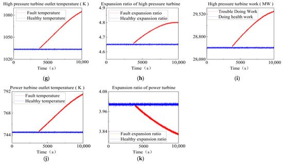
Figure 5.
Reaction of various components of the compressor fouling failure system. (a) Compressor outlet flow. (b) Compressor outlet temperature. (c) Compressor outlet pressure. (d) Compressor pressure ratio. (e) Combustion chamber outlet temperature. (f) Combustion chamber outlet pressure. (g) High-pressure turbine outlet pressure. (h) High-pressure turbine expansion ratio. (i) High-pressure turbine work. (j) Power turbine outlet temperature. (k) Power turbo expansion ratio.
4. Construction of Compressor Fouling Fault Early Warning Model
4.1. Data Preprocessing
In order to better simulate the working environment of the power system, noise disturbance is added to the input environment variables at the beginning of the simulation, which leads to some missing values and outliers in the simulation data. Noise was added to two key input environment variables at the model’s inlet: (1) inlet air temperature (T_in): Gaussian white noise with mean = 288 K (standard atmospheric temperature) and standard deviation = 2.88 K (1% of T_in); (2) inlet air pressure (P_in): Gaussian white noise with mean = 101.3 kPa and standard deviation = 1.013 kPa (1% of P_in). Therefore, data preprocessing to ensure the quality and accuracy of the data is the key link of fault diagnosis model modeling. As shown in Figure 6, the overall flow chart of data governance and uncertainty quantification is shown.
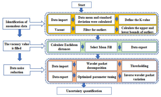
Figure 6.
Data Governance Flow chart.
Outliers are data points that deviate from the majority of observations in a dataset, potentially arising from measurement errors, data entry issues, or other anomalies, and they can adversely affect data analysis and model performance. Although the dynamic simulation model incorporates noise interference into the input variables to better reflect real-world measurement conditions and enhance engineering applicability, outlier detection remains necessary to ensure data quality. Therefore, outlier detection is performed on the raw data generated by the simulation to identify and handle such anomalous values before further analysis or modeling. This paper uses the standard deviation method to detect outliers in the dataset. Based on the mean and standard deviation of the data, the outliers are determined by measuring the difference between the data points and the mean. The deviation degree, also known as Z score, is calculated for each data point, using the following formula:
Among them, xi is the i th data point, µ is the mean value, and σ is the standard deviation.
The higher the Z score, the more likely it is to be marked as an outlier. At the same time, different standard deviation thresholds are selected to adjust the sensitivity of outlier detection.
In addition, the vacancy value is the missing information in the data, which may be caused by omissions, measurement errors, or other reasons. The appearance of the vacancy value will also have a great impact on the fault identification model. Before constructing the fault model of the collected data, it is necessary to adopt a reasonable method to process the vacancy value. The methods of processing the vacancy value include filling, deleting, or interpolation. In this paper, the KNN algorithm is used to fill the vacancy value. Through the form of hot deck filling, the most similar object is found in the complete data, and the current value is filled with the most similar value. Extract complete data from the global overall dataset to create a sound dataset R and calculate the Euclidean distance di between the missing target point and all individual data points in the sound dataset R, where the Euclidean distance calculation formula is as follows:
where Ai and Bi are two points in the dataset and n denotes the total number of features.
Screen the top k data points in ascending order according to the Euclidean distance di, calculate the weights of these k data points using the weighted value formula. To fill in the missing data value, perform a weighted operation on the k nearest neighboring points around the target missing point using the relevant formula to obtain the filled value F. The optimal number of neighbors, k, was determined individually for each monitoring parameter to account for differences in signal characteristics. A grid search was conducted over the range k = 1 to 20, and the value minimizing the root mean square error (RMSE) between predicted and observed values was selected for each measurement point. This adaptive selection strategy ensures robustness and accuracy in data restoration.
Additionally, noise in data refers to irrelevant information or random variations that may interfere with analysis and modeling. Although the addition of white noise does not affect the trend of parameters in this paper, data denoising is also performed to better fulfill future engineering applications. The Bayesian wavelet packet denoising adopted in this paper is a signal processing technique used to handle noise in signals. It combines wavelet packet transform with Bayesian estimation methods, aiming to extract useful information from observed signals and reduce the impact of noise. The multi-scale wavelet packet denoising method integrates the advantages of multi-scale characteristics, allowing for better processing of signals in multi-scale physical systems, and improves efficiency and accuracy through Bayesian methods. With the aid of auxiliary historical data, it is more suitable for signal processing and denoising tasks in different fields. By assuming that the actually measured process signal consists of two parts, namely the true process data and the noise signal, a measured signal can be expressed by the following formula:
The goal of denoising is achieved by continuously removing noise signals and preserving real data.
Finally, confidence intervals are used to quantify the uncertainty of data, so as to determine the range of the true values of estimated parameters. Based on sample data, this method can clarify the possible range of parameters and their corresponding confidence levels. In the final stage of data cleaning, quantitative verification of uncertainty is conducted on the cleaned data to evaluate its quality, accuracy, and reliability. This process ensures that no new problems are introduced in the cleaning steps, thus guaranteeing the validity of data.
4.2. Selection and Extraction of Fault Characteristic Parameters
As shown in Figure 7, after processing the data with outlier removal, missing value imputation, and wavelet packet Bayesian denoising, the uncertainty of the data is optimized by 98.8% compared with the original data, demonstrating improvement. These data preprocessing steps not only make the data more reliable but also improve the consistency and interpretability of the data. These improvements are not only conducive to a better understanding and analysis of the data but also help to accurately identify the hidden patterns and associations in the data, providing a more reliable basis for further data mining, analysis, and decision making.
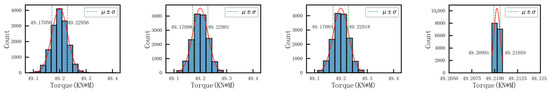
Figure 7.
Uncertainty quantification comparison chart.
Different types of equipment failures correspond to distinct characteristic parameters [35]. Therefore, the selection of appropriate characteristic parameters can effectively reflect the operating status and failure modes of the compressor. Through reasonable selection and analysis of characteristic parameters, it is possible to more accurately identify and address potential issues of the compressor, providing more effective support for system operation and maintenance.
This paper employs the Pearson correlation coefficient method to compare the correlation between five compressor parameters generated by the dynamic simulation model, namely compressor pressure ratio, compressor outlet flow, compressor outlet temperature, compressor power consumption, compressor outlet pressure, and compressor fouling faults. The correlation between the a-th column xa and the b-th column xb in the research matrix is calculated through the data matrix X = (x)m × n:
where m is the length of each column and the value range of the correlation coefficient is from 0 to 1. A value of 1 indicates perfect correlation, while a value of 0 indicates no correlation between columns.
Through the calculation of the Pearson correlation algorithm, the Pearson correlation coefficients of each parameter are obtained, so as to obtain the magnitude of the influence of each compressor parameter during the compressor fouling fault as shown in Figure 8.
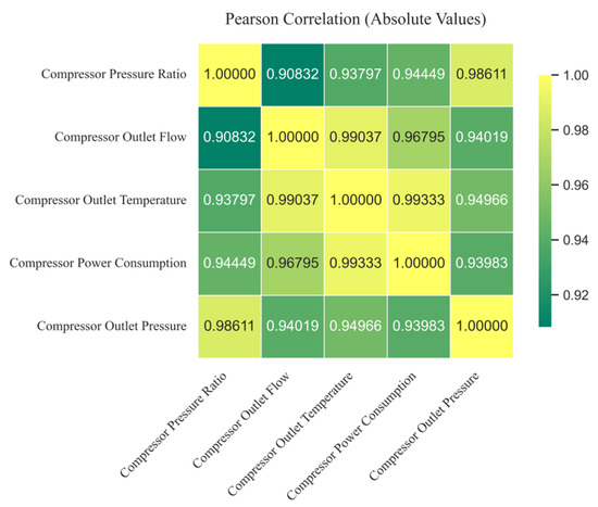
Figure 8.
Compressor parameters Pearson correlation plot set.
Therefore, the compressor outlet temperature was selected as the fault characteristic parameter. The finding that compressor outlet temperature is the parameter most sensitive to fouling was derived from a Pearson correlation analysis. Specifically, the correlation coefficients between each of the five compressor parameters and fouling severity were calculated across the simulation cases. As shown in Figure 8 and summarized in Table 3, compressor outlet temperature exhibited the highest average correlation coefficient (0.97428), followed by compressor power consumption (0.96912) and outlet flow rate (0.96138), indicating its superior sensitivity to fouling progression and justifying its selection as a key indicator for fault detection.
Table 3.
Statistical table of Pearson correlation of compressor parameters.
4.3. Modeling of the WPHM Reliability Model
The traditional Proportional Hazard Model (PHM), also known as the Cox model, is a semi-parametric regression model proposed by British statistician D.R. Cox [23]. This model exhibits strong adaptability, effectively utilizing the operational information of mechanical equipment to establish a connection between the operational status of a mechanical system and its overall failure life. It can analyze the influence of multiple factors on failure life without prior knowledge of the type of survival distribution. The WPHM has two key characteristics: (1) flexibility: the Weibull baseline distribution’s shape parameter (β) can describe different failure modes (β > 1: increasing failure rate, consistent with fouling; β = 1: constant failure rate; β < 1: decreasing failure rate); (2) interpretability: covariables (e.g., compressor outlet temperature) directly quantify their impact on failure rate via regression coefficients (α), enabling identification of key fault indicators [24]. The failure rate of this model is expressed as:
In the formula, λ0(t) represents the baseline failure rate, which is only related to the operating life t. g(X) is the covariate, indicating the degree of influence of various factors on the failure rate. A common form of the proportional hazard model is:
In the formula, X = (X1, X2, …, Xk) represents the covariables affecting the performance of the mechanical system, and α = (α1, α2, …, αk) denotes the regression coefficients corresponding to the covariables X.
Subsequently, the Weibull distribution is selected as the baseline distribution for survival time data. The Weibull distribution is frequently used in survival analysis to describe the probability distribution of time-to-event, and its probability density function is typically expressed in a parametric form, including a shape parameter and a scale parameter, which affect the shape and scale of the failure rate function, respectively. The expression for its failure rate is:
Subsequently, the WPHM equation is formulated by integrating the Weibull distribution with the proportional hazards model to form a unified equation, commonly referred to as the WPHM equation. This equation combines the failure rate function of the Weibull distribution with the covariate component of the proportional hazards model to establish an overall survival analysis model. The expression for its failure rate function is:
In the formula, β represents the shape parameter; η denotes the scale parameter; and t stands for time.
Finally, digital gas turbine data is selected for model adjustment, and the output failure probability is used for compressor fouling fault assessment. When the calculated failure rate exceeds the specified threshold, an alarm signal is issued. A compressor fouling fault early warning model as shown in Figure 9 is established.
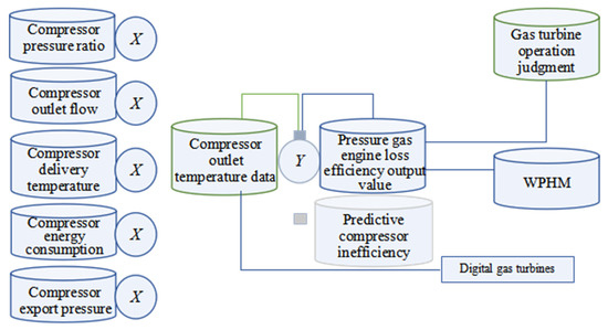
Figure 9.
Schematic diagram of the early warning model of fouling in compressor blades.
4.4. Fault Identification Results
During the system training and model optimization process, the Weibull Proportional Hazards Model (WPHM)-based early warning system was trained using simulation data from three distinct types of operational units: healthy units, units experiencing non-fouling faults, and units with only compressor fouling faults. This diverse dataset enables the model to effectively learn normal operational behavior, recognize fault-specific degradation patterns, and, crucially, distinguish compressor fouling from other fault types to minimize false alarms. The simulation data—generated from the MATLAB/Simulink dynamic model described in Section 2—were labeled based on predefined fouling thresholds (7% reduction in compressor flow rate and 2% reduction in efficiency), enabling supervised learning of degradation trajectories. These labeled data were then used to train and validate the WPHMs for each component, ensuring that the early warning system performs precise learning and reliable prediction based on realistic dynamic operation data, thereby enhancing its accuracy, robustness, and engineering applicability.
The WPHM was specifically configured to monitor compressor health by modeling the time-varying risk of failure. The baseline hazard distribution was assumed to follow a Weibull distribution, with the shape parameter β estimated via maximum likelihood estimation. Among multiple candidate parameters, compressor outlet temperature was selected as the primary covariate due to its highest Pearson correlation with fouling severity (0.97428), making it a sensitive indicator of performance degradation. The model parameters α and β were calibrated using data from simulation units to optimize the fit between predicted and actual fault onset times. In real-time operation, the trained WPHM computes a dynamic failure rate by comparing the current temperature trend against the learned baseline degradation profile. An early warning is triggered when this estimated failure rate exceeds a threshold.
According to Figure 10, the compressor fouling fault data is substituted into the WPHMs of each component for verification. The blue solid line in the figure represents the failure rate of the model, where a higher failure rate indicates a greater likelihood of component failure. Through experimental analysis of the training units and calculation verification of the test units, a failure probability of 0.15 is selected as the early warning threshold (shown as the yellow dashed line in the figure). This threshold enables early fault warning before failure, realizing condition monitoring of components. Meanwhile, a failure probability of 0.25 is selected as the failure threshold (shown as the red dashed line). When the failure probability exceeds this threshold, the unit is considered to be on the verge of failure. The red vertical line represents the actual failure time set in the simulation. It can be observed that only when the compressor fouling fault unit data is input into the compressor fouling fault WPHM does the fault curve rise, and the failure rate of the unit has increased before failure. This indicates that the model can monitor the occurrence of faults and accurately identify fault types, and the failure rate curve can describe the reliability of components.
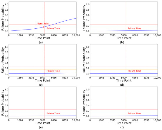
Figure 10.
The response of the fault identification model to each component when a compressor fouling fault occurs. (a) Compressor WPHM. (b) Propeller WPHM. (c) Dynamic turbine WPHM. (d) Combustion chamber WPHM. (e) Gearbox WPHM. (f) High-pressure turbine WPHM.
In addition, through model prediction and analysis of multiple simulated compressor fouling fault units, some early warning results are shown in Figure 11. Among all 24 compressor model units, the WPHM successfully provided early warnings for fouling faults across all validation datasets, except for Validation Dataset 3 of the WPHM compressor model. This finding demonstrates the outstanding accuracy and reliability of the prediction model in early identification of compressor fouling faults. This finding demonstrates that the WPHM early warning model for compressor fouling failure exhibits high reliability and accuracy in predicting fouling-related malfunctions, thereby providing support for failure prevention and maintenance in the dual-fuel power system.
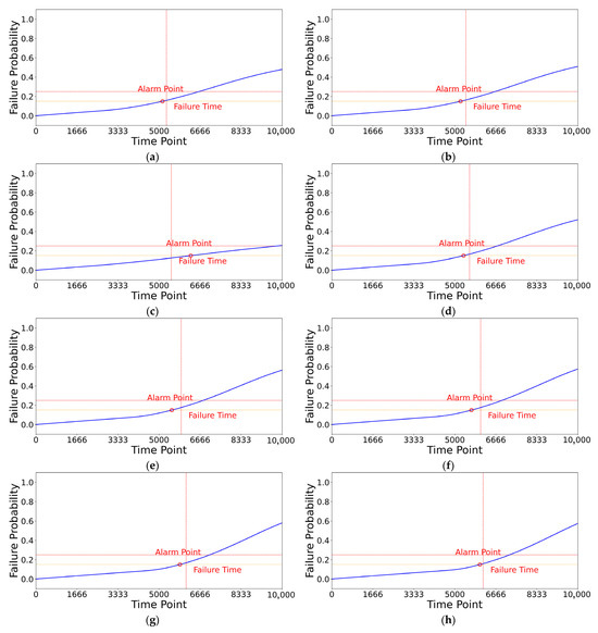
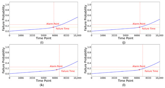
Figure 11.
Verification results of different fault simulation moment models(a) Compressor WPHM verification 1. (b) Compressor WPHM verification 2. (c) Compressor WPHM verification 3. (d) Compressor WPHM verification 4. (e) Compressor WPHM verification 5. (f) Compressor WPHM verification 6. (g) Compressor WPHM verification 7. (h) Compressor WPHM verification 8. (i) Compressor WPHM verification 9. (j) Compressor WPHM verification 10. (k) Compressor WPHM verification 11. (l) Compressor WPHM verification 12.
In summary, this compressor fouling fault prediction model demonstrates advantages in addressing compressor fouling issues. The method enhances the capability for fault prediction and diagnosis, thereby improving the reliability and operational efficiency of the power system while reducing maintenance and operational costs. Furthermore, the implementation of this method contributes to improving the overall performance of combined gas turbine systems. It also provides technical support for advancing intelligent equipment maintenance and automated management operations. This advancement supports ongoing technological progress in the energy sector. It also lays a foundation for sustainable development, showing promise in integrating advanced dynamic simulation techniques with health monitoring models for energy system applications.
5. Conclusions
This study establishes a compressor fouling fault signal simulation and identification model for combined gas turbine systems through the integration of WPHM with a dynamic simulation platform, yielding the following findings:
(1) This research employs a multi-component coupling methodology to construct a dynamic model of the complete dual-fuel power system. The holistic system modeling approach enables comprehensive analysis of compressor fouling impacts on overall powerplant performance, thereby establishing critical theoretical underpinnings and guidance for enhancing operational stability and system reliability in marine propulsion applications.
(2) This research conducts a simulation study on the compressor fouling fault in the dual-fuel power system. It not only focuses on the 5–7% decrease in the compressor’s flow rate but also reveals that this fault causes a 3–5% performance perturbation to other components of the system. This finding underscores the impact of compressor fouling on overall system performance and highlights the critical need for comprehensive system performance analysis and fault prediction.
(3) This study, following the implementation of outlier removal, missing value imputation, and wavelet packet Bayesian denoising, has achieved a 98.8% reduction in the uncertainty of each parameter compared to the original data, demonstrating improvement.
(4) The WPHM for compressor scaling faults was applied to validate the early warning system in a dual gas turbine power system. Results demonstrated that while Unit 3 failed to achieve normal early warnings, all other units successfully implemented the compressor scaling fault prediction. The accuracy rate for compressor scaling detection reached 95.8%, meeting practical engineering requirements.
6. Limitations and Future Work
6.1. Assumptions
(1) Fault Simulation Assumption: Compressor fouling was simulated as a gradual perturbation with a sine function—this assumes uniform particle accumulation, while actual fouling may be non-uniform (e.g., more accumulation on leading edges).
(2) Data Assumption: Noise was assumed to be Gaussian white noise—actual marine noise may include non-stationary components (e.g., vibration from waves).
(3) Model Assumption: The gas turbine model ignored minor components (e.g., fuel injectors, lubrication systems), which may have a small impact on overall performance but not on the main fouling mechanism.
6.2. Future Work
(1) Limitations: (a) The study used only simulation data—future work will integrate more measured data from actual marine turbines to improve model robustness. (b) It focused only on compressor fouling—future work will expand to other faults (e.g., turbine blade erosion, gearbox wear). (c) The WPHM used a single covariable (compressor outlet temperature)—future work will incorporate multi-variable models (e.g., combining temperature, pressure, and vibration) for higher accuracy.
(2) Future Work: (a) Conduct field tests on marine gas turbines to validate the model’s on-site applicability. (b) Develop a real-time early warning system based on edge computing, enabling on-board deployment. (c) Explore digital twin technology to integrate simulation models with real-time measured data for dynamic model updating.
Author Contributions
Conceptualization, Y.L.; methodology, H.S.; software, Y.C.; validation, Y.T.; formal analysis, L.D.; investigation, Y.P.; resources, Y.L.; data curation, X.J.; writing—original draft preparation, L.Z.; writing—review and editing, D.I.; visualization, H.S.; supervision, Y.L.; project administration, Y.L.; funding acquisition, Y.L. All authors have read and agreed to the published version of the manuscript.
Funding
This research was funded by the Fundamental Research Funds for the Central Universities (No. DUT25LAB110, DUT24LK008), the Open Research Fund of Hubei Technology Innovation Center for Smart Hydropower (No. SDCXZX-JJ-2023-01), and the State Key Laboratory of Clean and Effcient Turbomachinery Power Equipment (No. DEC8300CG202511985A1228194).
Data Availability Statement
The original contributions presented in the study are included in the article; further inquiries can be directed to the corresponding author.
Conflicts of Interest
Authors Yun Tan, Lunjun Ding, Youchun Pi, Linzhi Zhang were employed by the company China Yangtze Power Co., Ltd. The remaining authors declare that the research was conducted in the absence of any commercial or financial relationships that could be construed as a potential conflict of interest.
References
- Tu, P.; Yang, G.; Gao, L.; Liu, T.; Yang, S. Uncertainty effect of leading edge fouling on aerodynamic performance of compressor cascades. Aerosp. Sci. Technol. 2025, 162, 110235. [Google Scholar] [CrossRef]
- Rao, P.N.S.; Naikan, V.N.A. An optimal maintenance policy for compressor of a gas turbine power plant. J. Eng. Gas Turbines Power 2008, 130, 021801. [Google Scholar] [CrossRef]
- Templalexis, I.; Pachidis, V. Simulation of fouling in axial flow compressor using a throughflow method. J. Energy Eng. 2017, 143, 04016028. [Google Scholar] [CrossRef]
- Aldi, N.; Morini, M.; Pinelli, M.; Spina, P.R.; Suman, A.; Venturini, M. Performance evaluation of nonuniformly fouled axial compressor stages by means of computational fluid dynamics analyses. J. Turbomach. 2014, 136, 021016. [Google Scholar] [CrossRef]
- Xu, Z.; Chen, Y.; Zhao, H.; Chen, X.; Lu, Y. Research on the Early Warning and Broadcast of High-Pressure Turbine Thermal Corrosion Faults by Integrating Dynamic Simulation and Intelligent Identification. Appl. Math. Mech. 2025, 46, 999–1015. [Google Scholar] [CrossRef]
- Jin, J. Overview of the Numerical Propulsion System Simulation (NPSS) Program in the United States. Gas Turbine Test. Res. 2003, 16, 57–62. [Google Scholar]
- Yang, T.; Cai, J. Analysis of the Impact of Fouling on the Performance of Axial Flow Compressors. Aviat. Engine 2017, 43, 39–43. [Google Scholar] [CrossRef]
- Liu, J.; Ren, R.; Qiu, Y. Analysis of Surge Failure in Gas Turbine Compressors and Research on Surge Prevention Methods. Intern. Combust. Engine Power Devices 2016, 33, 1–4+32. [Google Scholar]
- Tarada, F.; Suzuki, M. External Heat Transfer Enhancement to Turbine Blading due to Surface Roughness. In Proceedings of the ASME 1993 International Gas Turbine and Aeroengine Congress and Exposition, Cincinnati, OH, USA, 24–27 May 1993. [Google Scholar] [CrossRef]
- Bons, J.P.; Taylor, R.P.; Mcclain, S.T. The Many Faces of Turbine Surface Roughness. J. Turbomach. 2001, 123, 739–748. [Google Scholar] [CrossRef]
- Lu, Y.; Zhang, M.; Chen, Y.; Ju, J.; Chen, F.; Bai, K.; Wang, X. A newly developed multi-strategy optimization algorithm framework based on the adaptive switching approach coupled with grey wolf optimizer. Knowl. Inf. Syst. 2025, 67, 5571–5617. [Google Scholar] [CrossRef]
- Lu, Y.; Guo, Z.; Zheng, Z.; Wang, W.; Wang, H.; Zhou, F.; Wang, X. Underwater propeller turbine blade redesign based on developed inverse design method for energy performance improvement and cavitation suppression. Ocean Eng. 2023, 277, 114315. [Google Scholar] [CrossRef]
- Chen, Y.; Lu, Y.; Cheng, J.; Guo, Y.; Zheng, Z.; Wang, X.; Jiang, X. T-BGA-CA: A Multi-Level Attention-Based BiGRU model for early fault warning in unmanned ocean platform electromechanical systems. Mech. Syst. Signal Process. 2025, 238, 113282. [Google Scholar] [CrossRef]
- Jiang, X.; Yang, S.; Wang, F.; Xu, S.; Wang, X.; Cheng, X. OrbitNet: A new CNN model for automatic fault diagnostics of turbomachines. Appl. Soft Comput. 2021, 110, 107702. [Google Scholar] [CrossRef]
- Jiang, X.; Wang, Z.; Chen, Q.; Cheng, X.; Xu, S.; Yang, S.; Meng, J. An orbit-based encoder–forecaster deep learning method for condition monitoring of large turbomachines. Expert Syst. Appl. 2024, 238, 122215. [Google Scholar] [CrossRef]
- Jiang, X.; Li, Y.; Wang, Z.; Hui, H.; Cheng, X. OrbitDANN: A Mechanism-Informed Transfer Learning Method for Automatic Fault Diagnosis of Turbomachinery. IEEE Sens. J. 2023, 24, 2228–2241. [Google Scholar] [CrossRef]
- Garg, S. Controls and health management technologies for intelligent aerospace propulsion systems. In Proceedings of the 42nd AIAA Aerospace Sciences Meeting and Exhibit, Reno, NV, USA, 5–8 January 2004; AIAA Paper: Reston, VA, USA, 2004; p. 949. [Google Scholar] [CrossRef]
- Lu, Y.; Jiang, S.; Che, Y.; Zhang, Z.; Wang, X. Coupling characteristics of the bowed micro-tubes for precooled heat exchangers under different inflow speeds. Phys. Fluids 2025, 37, 075155. [Google Scholar] [CrossRef]
- Lu, Y.; Shi, Y.; Cheng, X.; Zheng, Z.; Wang, T.; Wang, X.; Li, Y. Mechanism analysis of the bionic rudders on the operating performances of the high-speed autonomous underwater vehicle. Phys. Fluids 2025, 37, 085171. [Google Scholar] [CrossRef]
- Botros, K.K.; Kibrya, G.; Glover, A. A demonstration of artificial neural-networks-based data mining for gas-turbine-driven compressor stations. Eng. Gas Turbines Power 2002, 124, 284–297. [Google Scholar] [CrossRef]
- Tan, H.S. Fourier neural networks and generalized single hidden layer networks in aircraft engine fault diagnostics. J. Eng. Gas Turbines Power 2006, 128, 773–782. [Google Scholar] [CrossRef]
- Rajeev, V.; Roy, N.; Ganguli, R. Gas turbine diagnostics using a soft computing approach. Appl. Math. Comput. 2006, 172, 1342–1363. [Google Scholar] [CrossRef]
- Cox, D.R. Regression Models and Life-table. J. Am. Stat. Assoc. 1972, 2, 187–220. [Google Scholar] [CrossRef]
- Wang, F. Research and Application of Fault Feature Extraction and Intelligent Diagnosis Method for Non-Stationary Signals; Dalian University of Technology: Dalian, China, 2003. [Google Scholar]
- Banjevic, D.; Jardine, A. Calculation of reliability function and remaining useful life for a Markov failure time process. IMA J. Manag. Math. 2006, 17, 115–130. [Google Scholar] [CrossRef]
- Kang, Y.S.; Yoo, J.C.; Kang, S.H. Numerical predictions of roughness effects on the performance degradation of an axial-turbine stage. J. Mech. Sci. Technol. 2006, 20, 1077–1088. [Google Scholar] [CrossRef]
- Rowen, W.I. Simplifed mathematical representations of heavy-duty gas turbines. J. Eng. Gas Turbines Power 1983, 105, 865–869. [Google Scholar] [CrossRef]
- Rowen, W.I. Simplified mathematical representations of single shaft gas turbines in mechanical drive service. In Turbo Expo: Power for Land, Sea, and Air; American Society of Mechanical Engineers: New York, NY, USA, 1992; Volume 78972. [Google Scholar] [CrossRef]
- Camporeale, S.M.; Fortunato, B.; Dumas, A. Dynamic modelling of recuperative gas turbines. Proc. Inst. Mech. Eng. Part A J. Power Energy 2000, 214, 213–225. [Google Scholar] [CrossRef]
- Zheng, W.; Wang, P. Research on High-Precision Modeling Methods for Dual-Shaft Gas Turbines. Therm. Energy Power Eng. 2016, 31, 19–24, 121–122. [Google Scholar] [CrossRef]
- Guo, C.; Huang, L.; Tian, K. Combinatorial optimization for UAV swarm path planning and task assignment in multi-obstacle battlefield environment. Appl. Soft Comput. 2025, 171, 112773. [Google Scholar] [CrossRef]
- Zhou, R.; Kang, Y. Fault Early Warning of Gas Turbine Combustion Chamber Based on CNN-LSTM. Therm. Energy Power Eng. 2024, 39, 191–197+215. [Google Scholar] [CrossRef]
- Qu, Y.; Li, T.; Fu, S.; Wang, Z.; Chen, J.; Zhang, Y. A mechanical fault diagnosis model with semi-supervised variational autoencoder based on long short-term memory network. Nonlinear Dyn. 2024, 113, 459–478. [Google Scholar] [CrossRef]
- Li, S. Simulation Technology of Ship Power Plant; Harbin Engineering University Press: Harbin, China, 2013. [Google Scholar]
- Lin, X. Performance Simulation and Fault Characteristic Research of Dual-Shaft Gas Turbines; Beijing University of Chemical Technology: Beijing, China, 2021. [Google Scholar]


Disclaimer/Publisher’s Note: The statements, opinions and data contained in all publications are solely those of the individual author(s) and contributor(s) and not of MDPI and/or the editor(s). MDPI and/or the editor(s) disclaim responsibility for any injury to people or property resulting from any ideas, methods, instructions or products referred to in the content. |
© 2025 by the authors. Licensee MDPI, Basel, Switzerland. This article is an open access article distributed under the terms and conditions of the Creative Commons Attribution (CC BY) license (https://creativecommons.org/licenses/by/4.0/).