Investigation on the Use of 2D-DOST on Time–Frequency Representations of Stray Flux Signals for Induction Motor Fault Classification Using a Lightweight CNN Model

Abstract

Condition monitoring and fault detection in induction motors (IMs) are priorities in the industrial environment to secure safe conditions for the processes and production. Convolutional Neural Networks (CNNs) are gaining interest in these tasks as they allow automatic extraction of features from the inputs, sometimes Time–Frequency Distributions (TFDs) obtained with various transforms, directly into large models for data classification. This work presents a proposal for the application of a widely used texture analysis tool in the medical field, the 2D Discrete Orthonormal Stockwell Transform (2D-DOST), to improve the accuracy of a lightweight CNN when using different TFDs and comparing the results to the use of the TFDs in RGB and grayscale. The results show that the use of the 2D-DOST improves the classification accuracy in a two to five percent range for all motor conditions under study, while having minimal variations to the training times when compared to RGB or grayscale images, opening the possibility for the use of image processing tools on TFDs to improve automatic feature extraction while using small CNN models.

1. Introduction

The extensive use of induction motors (IMs) in the industrial environment due to their robustness, flexibility of application for a vast number of tasks and mechanisms makes them a priority for maintenance and condition monitoring, as the presence of faults could lead to performance reduction, increments in production costs, and catastrophic failure of the machines in the worst-case scenario [1,2]. Condition monitoring and fault detection are important tasks in the industry due to their connection to predictive maintenance, minimizing production downtime, improving maintenance and production efficiency, protecting the equipment and increasing safety in the workplace. For many years, these areas have been of great interest for researchers and industry, developing a plethora of techniques and methodologies to detect and identify the apparition of irregularities in the physical magnitudes available for the monitoring of the IMs (e.g., stator current, vibration signals, temperature, acoustic emissions, voltages, electrical power and, in more recent times, magnetic flux) and relate these variations to the emergence of mechanical or electrical faults by means of temporal, spectral or statistical analysis, as well as automated processing techniques like Machine Learning (ML) and Deep Learning (DL) [1,2,3,4,5]. Convolutional Neural Networks (CNNs), one of the most popular DL tools, allow for the automatic extraction of features from the 1-D or 2-D inputs and achieve great classification results without the need for expert knowledge, and when paired with Time–Frequency Distribution (TFD) images, have become a growing trend for fault diagnosis.

One of the components of an IM that attracts more attention is the bearings, as they represent up to 40% of the reported faults [1], with vibration signals as the preferred source of information for diagnosis. Many approaches have been presented, like the one in [6], where the authors analyzed the HUST dataset applying Multitask Learning (MTL) to diagnose six faulty conditions with only one severity on different types of bearings, using the Continuous Wavelet Coefficient Maps (CWCMs) as inputs to a Long Short-Time Memory (LSTM) + CNN model. In [7], a comparison between different TFDs on the Case Reserve Western University (CRWU) bearing dataset and experimental results showed that the use of the Fourier Synchrosqueezed Transform (FSST) on vibration signals achieved great performance when feeding 3-channel images of 28 × 28 pixels to a CNN, outperforming other popular TFDs, such as the Continuous Wavelet Transform (CWT) or the Short-Time Fourier Transform (STFT). However, in [8], a similar approach is presented for bearing fault diagnosis, using Transfer Learning (TL) and RGB images of 224 × 224 pixels, with the authors concluding that the CWT and FSST performed better than other TFDs. The superiority of the FSST for bearing diagnosis is confirmed in [9], where the authors compared its performance against the Wavelet Synchrosqueezed Transform (WSST) on the CRWU dataset, and in [10], where current signals went through the FSST and Hilbert Envelope Spectrum for diagnosing an outer race (OR) defect on bearings, identifying the related frequency component with ease. With a different approach, the authors of [11] rearranged 1-D signals from different sensors and different natures to 2-D matrices, then assembled them to generate 120 × 120 inputs for a CNN model, obtaining good classification results for five faulty bearing conditions, highlighting that the reduction in the model parameters leads to a reduction in classification accuracy. In a similar manner, the work reported in [12] presents a comparison of sound and vibration signals from the CWRU and National Aeronautics and Space Administration (NASA) datasets, analyzed by the Wavelet Scattering Transform (WST) and the Adaptive Superlet Transform (ASLT) to generate RGB and grayscale images of five sizes ranging from 16 × 16 to 224 × 224 pixels and classified by a hybrid CNN–Support Vector Machine (SVM) model, achieving better performance with the biggest images in grayscale for the diagnosis of three bearing conditions. The authors of [13] developed a system based on the Internet of Things (IoT) technology for bearing fault detection using the STFT to process vibration signals, diagnosing the conditions by means of a CNN model with three convolutional and pooling layers with different kernel sizes, achieving a methodology that could be implemented online and offline. In [14], the authors created a Graph Convolutional Network (GCN) to tackle bearing fault detection and Remaining Useful Life (RUL) estimation using vibration signals from a motor under different operating conditions, obtaining good results in both tasks with a novel DL method. A different approach is found in [15], where the authors filtered the fundamental component from current signals to identify the harmonics related to different bearing conditions using both the CWT and STFT and compared the diagnostic performance of five CNN models extensively used in the literature, finding an improvement over non-filtered signals.

Other conditions studied with this kind of approach include broken rotor bars (BRBs), as reported in [16], where the authors analyzed current signals using the STFT on the transient state, achieving good results for the diagnosis of four conditions with 25 × 25 grayscale images and a compact CNN model. Similarly, the author of [17] developed a method to diagnose five BRB conditions from STFT images from vibration signals, using TL with four well-known CNN models and showing an improvement in detection accuracy over a CNN model that was not previously trained. Faults related to the kinematic chain connected to the IM have also been diagnosed, as reported by the authors of [18], where gearbox wear was identified by the analysis of stray flux signals using a variant of the Multiple Signal Classification (MUSIC) algorithm, the Short-Time MUSIC (ST-MUSIC). Also, other investigated faults, such as eccentricities and misalignment, were studied by the authors of [19] using the Persistence Spectrum to stray flux signals, generating 224 × 224 RGB images that fed a CNN model, allowing the detection of 5 different conditions related to these faults.

Similarly, TFDs and CNNs have been used to identify faults of different origins in IMs. One example of this is the research presented in [20], where the authors applied the CWT on vibration and current signals to diagnose six different conditions in an IM: healthy, shorted turns, unbalanced, bearing’s inner race (IR), BRB and bent rotor; the results suggested that the use of 128 × 128 grayscale images, the fusion of the signals and features improved the diagnosis. The authors of [21] presented a comparison of four TFDs for the diagnosis of a BRB, imbalance, and bearing defects using vibration signals, offering an analysis of the way these TFDs display the information and concluding that the ST-MUSIC gives more detailed information about the components related to the faults under study. In [22], the authors used current signals from multiple sensors to diagnose BRB and bearing faults in a motor, transforming the 1-D signals to 224 × 224 RGB images fed to a TL-deep CNN (dCNN) model, obtaining a good performance using a larger CNN model when compared to other popular tools.

It has been seen that the use of TFD as inputs for CNN has become a trend for fault diagnosis; however, most of the time, the images are used directly as obtained, in RGB or grayscale, without a processing step that could improve the identification of the conditions under study, as in other fields. One technique that has shown improvements in the medical diagnosis area is the use of the 2-D Discrete Orthonormal Stockwell Transform (2D-DOST); this transform provides local spatial frequency information from images that can be used to characterize the horizontal and vertical frequency patterns and obtain sets of texture features [23]. This technique has been used to diagnose multiple medical conditions, as in [24], where the authors applied it to Magnetic Resonance Images (MRIs) to diagnose eight conditions using CNNs, outperforming other established methodologies in the area. The authors of [25] used the DOST to analyze multiple sclerosis MRIs and compare the results to the Polar Stockwell Transform (PST), finding a slight advantage when using the PST; on the other hand, in [26], the authors proposed a fusion methodology considering the 2D-DOST, the Orthogonal Ripplet II Transform (ORTII) and the original MRIs for the classification of Alzheimer’s disease using a CNN model, concluding the improvement of the results with the fusion of the extracted features. The 2D-DOST has been used in cancer prognosis [27], glioblastoma prediction [28], and seizure identification from MRIs during pregnancy [29].

Considering the aforementioned, it is evident that the use of CNNs and TFDs for the diagnosis of a variety of fault conditions in IMs is a growing trend; however, most works focus on a particular component or type of faults, relying primarily on well-known databases with no empirical experimentation, employing vibration and current signals, whose sensors can be invasive, as preferred information sources; and using TFD images of considerable size with no extra processing and large CNN models for classification. In a recent work [30], the authors explored the use of the 2D-DOST on STFT and CWT images from stray flux signals for the diagnosis of bearing faults in an IM with a lightweight CNN model, identifying an improvement in accuracy when applying the 2D-DOST to the grayscale CWT images, while the opposite was observed on the STFT dataset. In this paper, a continuation of the previous work is carried out, proposing a methodology where stray flux signals are analyzed using the STFT, CWT, FSST and ST-MUSIC to generate TFDs, which are then saved in RGB, grayscale and a third set processed with the 2D-DOST for the diagnosis of one healthy and eleven faulty conditions including bearing faults, various severities of BRBs, unbalances, misalignments and a loosened bolt. The results compare the performance on several configurations of TFDs and image types, including training times, accuracy, and the effect of processing tools on the inputs of a lightweight CNN model. With these results, the proposed method presents an alternative to improve the classification accuracy of a small CNN model for multiple fault diagnosis considering the use of various TFDs by employing a texture analysis tool as a preprocessing step in the analysis of stray flux signals using non-invasive sensors.

2. Materials and Methods

In this section, the theoretical background of the tools and techniques used in this research, as well as the methodology employed for the analysis of the stray flux signals and the diagnosis of motor fault conditions are described.

2.1. Theoretical Background

In this subsection, the theoretical fundaments and mathematical description of the tools employed are presented. First, fault-related frequency components are summarized, as traditional methodologies focus on the detection of these components for the diagnosis of faults in IM using frequency- or time–frequency domains. Secondly, TFDs previously discussed as tools for fault detection using CNNs are described, being the basis of the proposed methodology, as well as the 2D-DOST, which was commented to be used as a texture analysis tool in medical image processing and is intended to serve as a preprocessing step to identify its capabilities to improve fault diagnosis using a CNN model.

2.1.1. Fault Detection in Induction Motors

The presence of a faulty condition in an IM changes the way it behaves, and it can be reflected in the physical magnitudes that can be measured from the motor. Throughout the years, researchers have identified the frequency components related to the most common faults in vibration and current signals, which are the preferred sources for diagnosing IMs, and more recently, stray-flux analysis has been applied to this end.

Table 1. Fault frequency component equations for different signals.

Fault	Equation		Signal	Source
Outer Race Bearing Fault	$f_{ov}={\displaystyle \frac{N_b}{2}}{f}_r\left(1-{\displaystyle \frac{D_b}{D_c}}cos\beta \right)$	(1)	Vibration	[1,3,4]
	$f_{oc}=|f_s\pm k\ast f_{ov}|$	(2)	Current and flux	[1,5]
Broken Rotor Bar	$f_{brb}=f_s\left(1\pm 2\ast k\ast s\right)$	(3)	Vibration and current	[1,3,4]
	$f_{brb}=f_s\pm k\ast f_r$	(4)	Airgap flux	[5]
	$f_{brb}=\left\{\begin{array}{c}{f}_s\left(1\pm 2\ast k\ast s\right)\\ f_s+f_r\pm 2\ast k\ast s\ast f_s\end{array}\right.$	(5)	Radial stray flux	[5]
	$f_{brb}=\left\{\begin{array}{c}s\ast f_s\\ 3\ast s\ast fs\end{array}\right.$	(6)	Axial stray flux	[5]
Eccentricity and Misalignment	$f_{ecc}=f_s\pm f_r(k\ast N_r\pm n_d)$	(7)	Magnetic flux	[5]
	$f_{ecc}={2\ast f}_s\pm f_r$	(8)	Vibration	[1]
	$f_{e-m}=f_s\pm k\ast f_r$	(9)	Current and flux	[1,19]
	$f_{e-m}=f_s(1\pm k\ast s)$	(10)	Current	[31]

summarizes the frequency components in the vibration, current, and magnetic flux signals related to the faults considered in this research, which are extensively used in the literature for the diagnosis of fault conditions in IMs through spectral analysis and frequency decomposition methods. Equations (1)–(10) consider f_ov as the frequency related to OR defects in vibration signals; f_oc as the frequency related to OR in electrical signals; f_brb as the components related to BRB; f_ecc as the component related to eccentricities; f_e − _m as a component related to both eccentricity and misalignment; f_s as the supply frequency; f_r as the rotational frequency of the rotor; s as the slip of the machine; k as an integer k = 1, 2, 3, …; N_b as the number of balls in the bearing; D_b as the diameter of the balls; D_c as the pitch or cage diameter; β as the contact angle between a ball and the raceway; N_r as the number of rotor slots; n_d = 0 for static eccentricity; and n_d = 1, 2, 3, … for dynamic eccentricity.

2.1.2. Short-Time Fourier Transform (STFT)

The STFT is a widely used TFD, which performs the Fourier Transform of a signal using a fixed size sliding window, granting the capability to obtain both time and frequency information, allowing the detection of transient phenomena. Equation (11) shows the mathematical definition of the STFT, where x(t) is the time-domain signal, h(τ − t) is the window function centered at time t, and ω represents the angular frequency [32,33].

$$STFT\left(\tau ,\omega \right)=\underset{-\infty }{\overset{+\infty }{\int }}x\left(t\right)h\left(t-\tau \right)e^{-j\omega t}dt$$

(11)

2.1.3. Continuous Wavelet Transform (CWT)

The CWT was developed to tackle problems related to the fixed resolution of STFT, presenting an alternative capable of multi-resolution analysis thanks to the use of the mother wavelet functions that adapt to the changes in frequency, making it adequate for the analysis of non-stationary signals. Equation (12) presents the definition of the CWT, where x(t) is the signal in the time domain, C_w(a, b) is the function of the scale (a) and translation (b), and ψ is the mother wavelet function [8,34].

$$C_w\left(a,b\right)={\displaystyle \frac{1}{\sqrt{a}}}\underset{-\infty }{\overset{+\infty }{\int }}x\left(t\right)\psi \ast \left({\displaystyle \frac{t-b}{a}}\right)dt$$

(12)

2.1.4. Fourier Synchrosqueezed Transform (FSST)

The Synchrosqueeze Transform is a post-processing method that aims to provide a sharper, more concentrated representation of multicomponent signals in the TFDs from linear transforms, granting major separation between the frequency components and demodulation of the different modes in the signal while being a reversible process [29], producing a higher frequency and time resolution compared to other techniques [30]. The FSST applies the Synchrosqueezing process to the STFT, producing a sharper spectrogram with narrower components, with the mathematical definition in Equation (13), where V_gf(t,η) is the STFT of a function (or signal) f filtered at a frequency η using the spectral window g; ω and t correspond to the observed time and frequency, respectively; and Ωgf(t,η) represents the instantaneous frequency obtained using phase transform [7,35,36].

$$FSST=\underset{-\infty }{\overset{+\infty }{\int }}{V}_{g}f\left(t,\eta \right)\delta \left(\omega -\Omega gf\left(t,\eta \right)\right)d\eta$$

(13)

2.1.5. Short-Time Multiple Signal Classification

MUSIC algorithm is a high-resolution method capable of detecting frequency components in signals with important levels of noise [21,37]. This algorithm considers that the discrete time signal x[n] can be represented as the sum of m complex sinusoids in noise e[n], as shown in Equations (14) and (15), where N is the number of samples in the signal; n = 0, 1, 2, …, N – 1; B_i is the complex amplitude of the i-th complex sinusoid with frequency f_i; and e[n] is a sequence of white noise with zero mean and unit variance σ².

$$x\left[n\right]=\sum _{i=1}^m\overline{B_i}{e}^{j2\pi f_{i}n}+e[n]$$

(14)

$$\overline{B_i}=\left|B_i\right|e^{{\phi }_i}$$

(15)

Equation (16) presents the autocorrelation matrix, R, of the noisy signal x[n] as the sum of the autocorrelation matrices of the pure signal, R_s, and the noise, R_n, with P as the number of frequencies; the exponent H as the Hermitian transpose; I corresponding to the identity matrix; and e^H(f_i) as the signal vector as given by Equation (17).

$$R=R_s+R_n=\sum _{i=1}^P{\left|B_i\right|}^2{e}^H\left(f_i\right)+{\sigma }_n^{2}I$$

(16)

$$e^H\left(f_i\right)=\left[1 e^{-j2\pi f_i} \dots e^{-j2\pi f_i(N-1)}\right]$$

(17)

From the orthogonality condition of both subspaces, the MUSIC pseudospectrum Q is given by Equation (18), where V_m+1 is the noise eigenvector, and exhibits peaks that correspond to frequencies of principal sinusoidal components, where e(f)^HV_m+1 = 0.

$$Q^{MUSIC}\left(f\right)={\displaystyle \frac{1}{{\left|e{\left(f\right)}^H{V}_{m+1}\right|}^2}}$$

(18)

To capture the time information, the signal is analyzed using a sliding window, obtaining the MUSIC pseudo-spectrum of each window, and condensing the information to form a TFD that preserves the information and reduces the noise present in the signals while evidencing large components [37].

2.1.6. Two-Dimensional Discrete Orthonormal Stockwell Transform

Stockwell Transform (ST) was introduced in 1996 in [38], originating from the STFT and the CWT, providing an alternative with high time and frequency resolutions at low frequencies and high time resolution at high frequencies by using a window of variable length [20]. The original definition of the ST presented a high redundancy, which affected computational cost; this problem led to the development of mathematical formulations to reduce the computational cost, with the DOST being one of the most used, having the computational cost of the Fast Fourier Transform (FFT) [39]. Equation (19) presents the mathematical definition of the 2D-DOST, where considering a N × N image f(x,y), F(m,n) is the 2D Fourier Transform of the image f, u and v are the shift parameters that control the center of the window on the x- and y-axis, f_u and f_v are the frequencies related to scale parameters, v_x and v_y are the horizontal and vertical frequencies, respectively, p_x and p_y = 0, 1, …, log(N − 1).

$$S\left(u,v,f_u,f_v\right)={\displaystyle \frac{1}{\sqrt{2^{p_x+p_y-2}}}}\sum _{m=-2^{p_x-2}}^{2^{p_x-2}-1}\sum _{n=-2^{p_y-2}}^{2^{p_y-2}-1}F\left(m+v_x, n+v_y\right)e^{\left(2\pi j\left({\displaystyle \frac{m\ast u}{2^{p_x-1}}}+{\displaystyle \frac{n\ast v}{2^{p_y-1}}}\right)\right)}$$

(19)

The resulting image, S, has the same size as f, and contains information about the frequencies (f_u, f_v) in the bandwidth of 2^{px − 1} × 2^{py − 1} [24].

2.2. Proposed Methodology

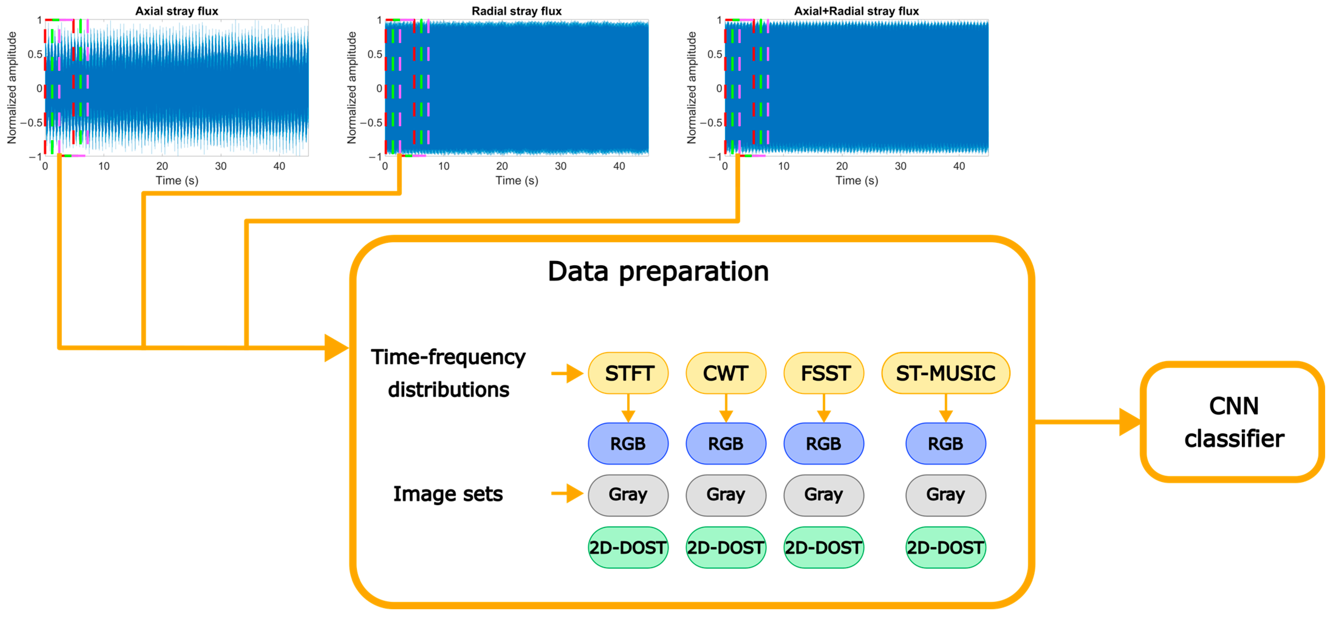
Figure 1 shows a block diagram illustrating the stages included in the methodology. The first step is normalizing the stray flux signals to a [−1, 1] amplitude range; then, the signals are windowed, considering 5 s segments and a 1 s window displacement. Each window is processed in the second stage to generate time–frequency representations for the analysis using the STFT, the CWT, the FSST, and the ST-MUSIC; the representations are then saved as RGB images of 64 × 64 pixels and converted to grayscale. Additionally, the grayscale images undergo a 2D-DOST postprocessing to generate new images. All three sets are then fed to a lightweight CNN model to classify the data into twelve different motor conditions; this process is repeated for each TFD and image set.

Experimental Setup

The experiments were conducted on a 1 hp, six-pole, three-phase induction motor with a rated speed of 1140 rpm, line-fed with 460 V at 50 Hz. The motor was coupled to a generator, acting as a load, and all tests were performed at the nominal load level. For the acquisition of the stray flux signals, a three-axis magnetometer was employed, model DM1422AGMV with a range of ±1200 µT and a 0.042 µT/LSB sensitivity at a sampling rate of 1 kHz, allowing for the measurement of the axial and radial flux components, as well as the combination of both in an orthogonal axis. This sensor was placed centered on the side of the IM, as is common practice, since it can measure in the three orthogonal axes from a single spot and that position allowed for better measurements.

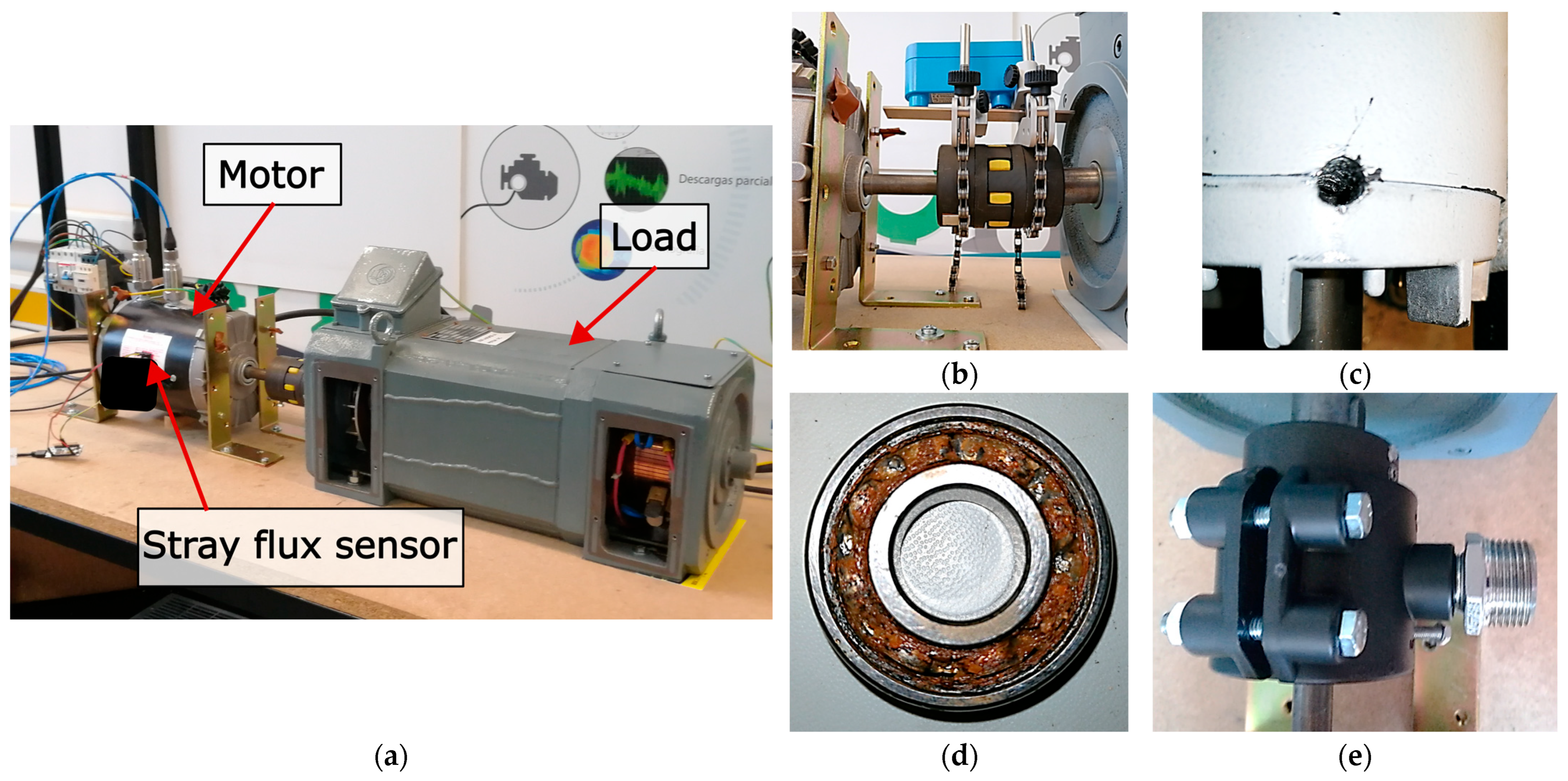
In this study, one “healthy” (HLT) condition and eleven faulty conditions were considered. The faulty states could be grouped according to the source of the fault: bearings, rotor, misalignment, unbalance of the load, and attachment to the test bench. For the bearing-related faults, bearings model NSK-6203 DU, with a 17 mm internal diameter, a 40 mm external diameter, and eight balls were used; the conditions included a 1 mm OR hole, no grease (NG), and induced corrosion by submerging the bearing in brine for one (COR0) and two days (COR1), respectively, followed by three days of drying. The rotor-related conditions considered were one and two broken rotor bars (1BRB and 2BRB, respectively), induced by drilling small holes in the rotor bars. For the misalignment conditions, three angular deviations were caused by placing shims under the motor’s feet: 0.8° (Mal0.8), 1.24° (Mal1.24), and 1.6° (Mal1.6). The unbalanced conditions were created by using an asymmetric coupling between the motor and the load (UNB0), applying a mass of 5.25 g with a center of mass at a 7.25 mm radius from the center of the shaft, and attaching weight to the asymmetric coupling (UNB1), applying a mass of 99.35 g with a center of mass at a 21.45 mm radius from the center of the shaft. Finally, for the last condition, a bolt fixing the motor to the test bench was loosened to create minor disturbances to the system (LB). Figure 2 shows the test bench and some conditions and elements used for the experiments. For each condition, six tests were performed, capturing three stray flux signals for 45 s of the steady state per test.

The data was processed in a personal computer CPU i9-13980HX 2.2 GHz, 32 GB RAM, a NVIDIA GeForce RTX 4060 Laptop GPU in the platform Matlab 23.2.0.2859533 (R2023b) Update 10. The CNN model consisted of an 11-layer structure defined in

Table 2. Structure of the implemented CNN model.

Layer	Structure
	Layer Type	Size	Number of Filters/Strides
1	Image Input	64 × 64	-
2	Convolution	3 × 3	8
3	Batch Normalization	-	-
4	ReLU	-	-
5	Max Pooling	2 × 2	2
6	Convolution	3 × 3	8
7	Batch Normalization	-	-
8	ReLU	-	-
9	Fully Connected		-
10	SoftMax	-	-
11	Classification	12	-

, which was trained using a Stochastic Gradient Descent with Momentum method, considering a learning rate of 0.001, a mini batch size of 30, a maximum of 5 epochs, and a validation frequency of 30. Because in the experiments RGB and grayscale images were considered, the size of the Input Layer changed according to the number of layers of the image, and the datasets were divided randomly with a distribution of 60% for training, 20% for validation, and 20% for testing. The model has 99.1 k learnable parameters, significantly less than well-known models like GoogLeNet with 6.9 M, AlexNet with 60.9 M, ResNet18 with 11.6 M, ResNet50 with 25.5 M, or VGG-16 with 138.3 M; this difference situates the proposed model as a lightweight model due to its reduced size and number of parameters [40].

3. Results

In this section, the results obtained with the previously established methodology are described, starting from the image generation to the classification process and comparing the performance in the fault identification process for each dataset.

3.1. Image Generation

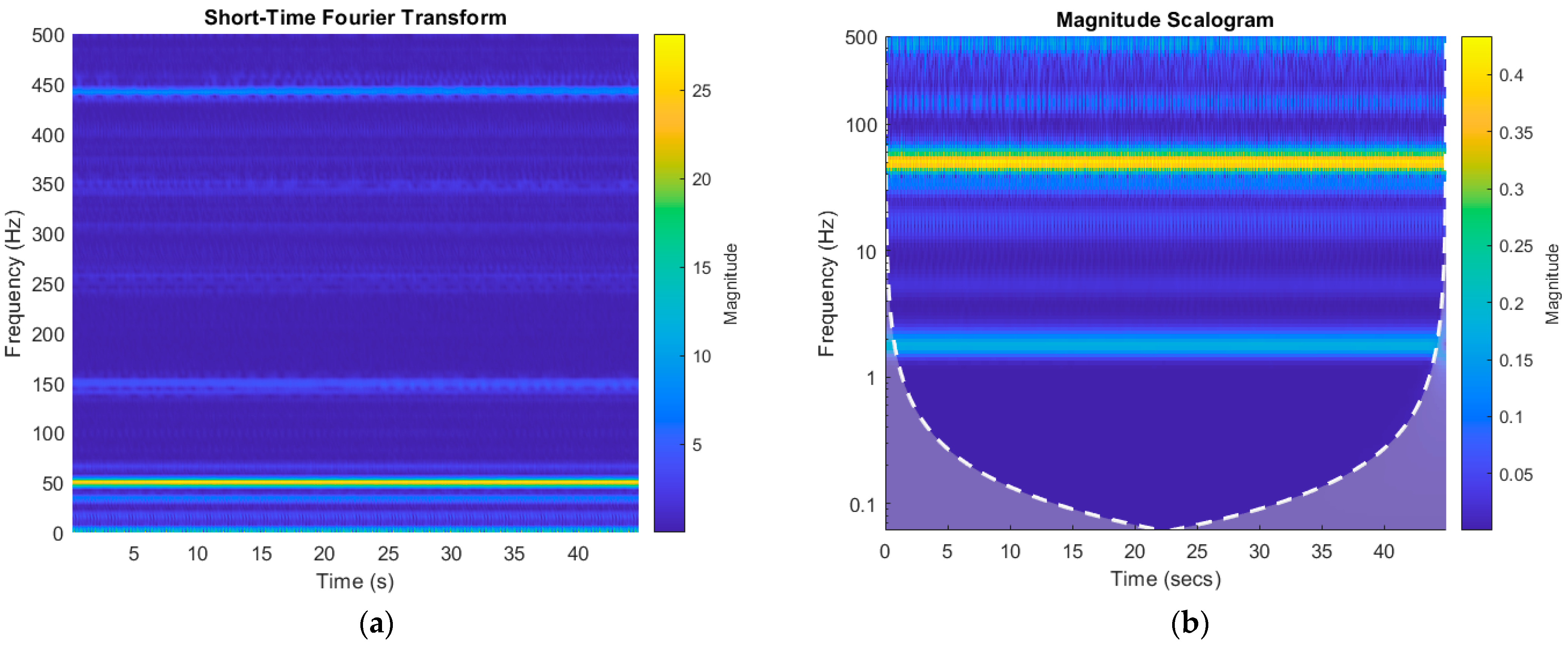
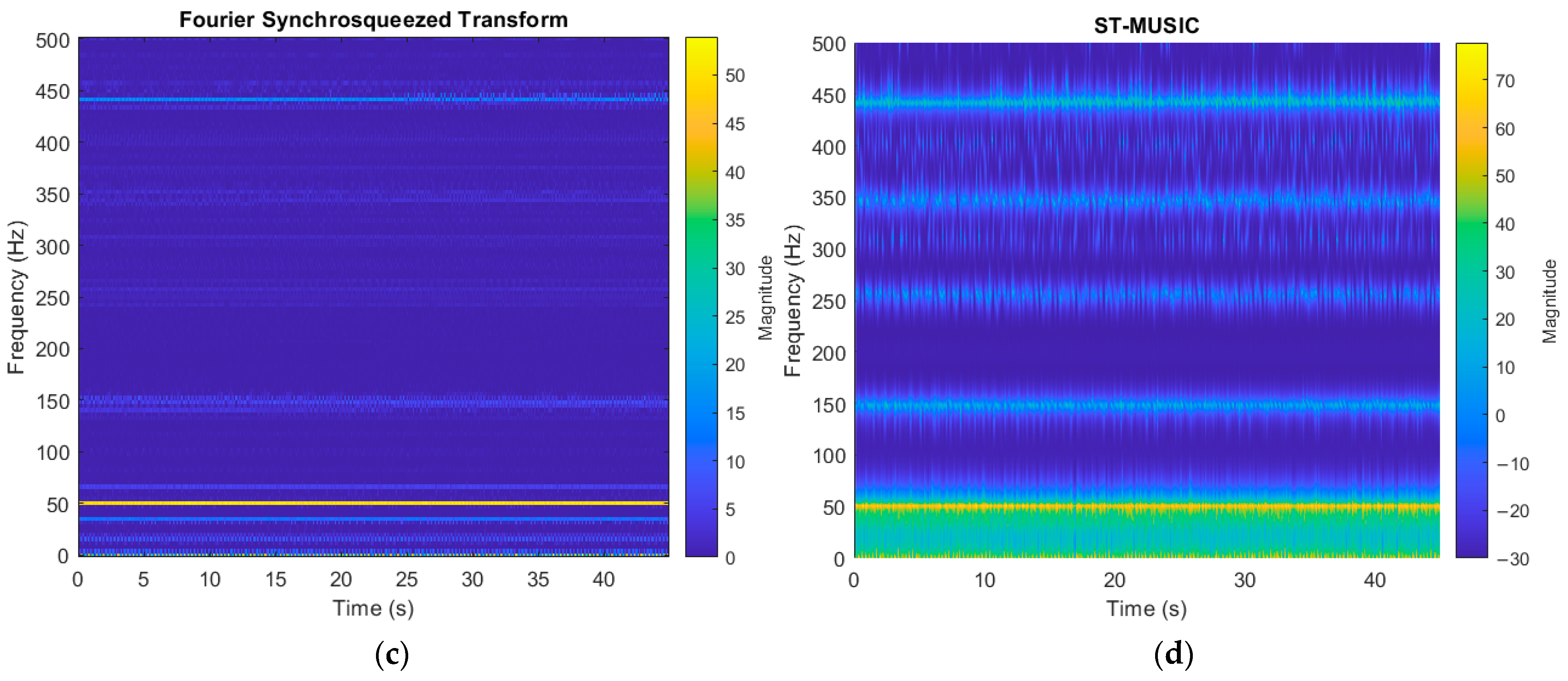
The stray flux signals obtained from the experiments conducted in a laboratory were processed following the methodology defined in Section 2.2. Each of the transforms considered similar parameters; for the CWT, a Morlet mother wavelet was considered; for the STFT, FSST and ST-MUSIC, windows of 256 samples were considered. Additionally, in all cases, the representations considered a frequency range from 0 to 500 Hz, although the CWT representation considers a logarithmic distribution in the frequency axis, differing from the other transforms in data distribution but conserving its distinctive characteristic, as appreciated in Figure 3, where TFDs for a whole signal are displayed.

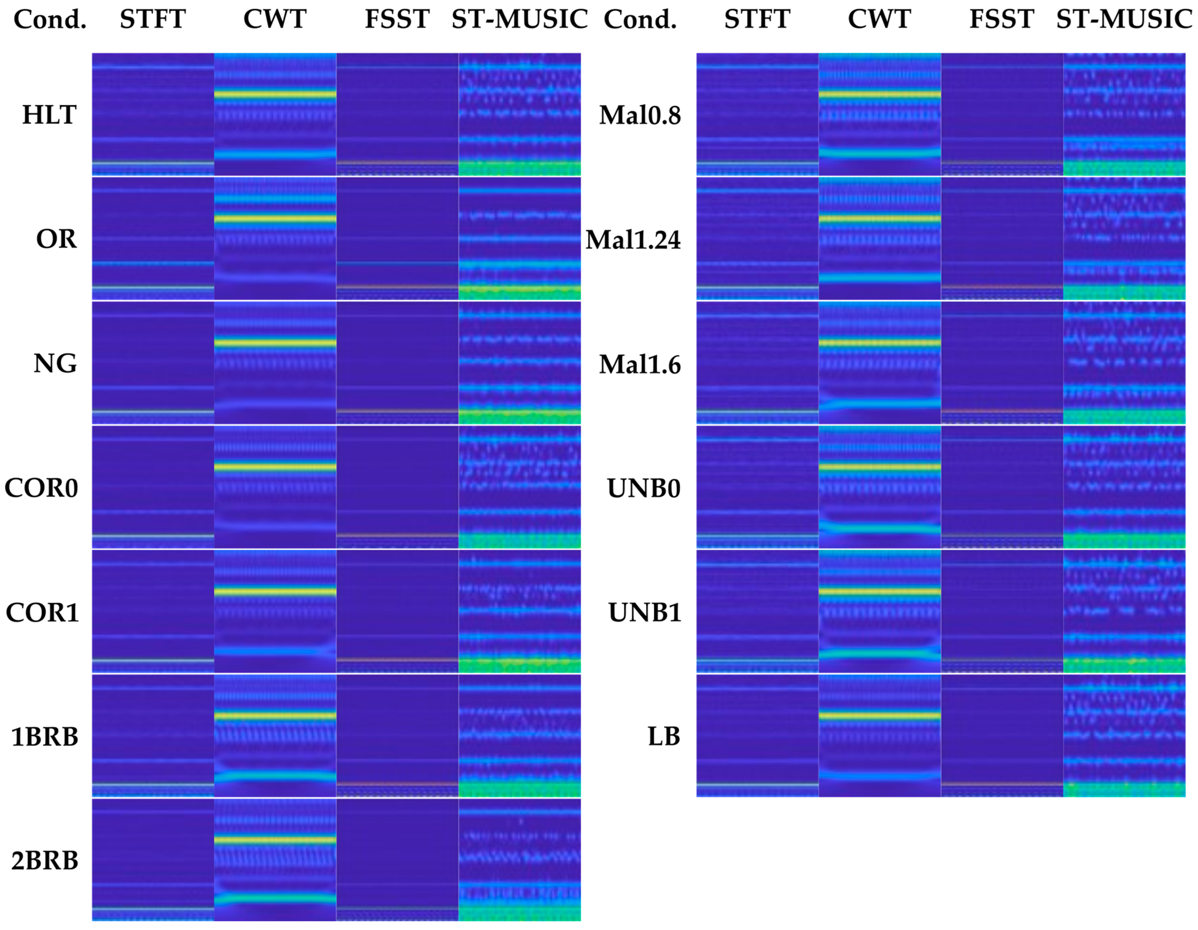
The time–frequency diagrams were then adapted and saved for further processing as mentioned in the methodology, obtaining just the area of importance and resizing the pictures to a 64 × 64 resolution. Considering the three stray flux signals and the window’s length and overlap, a total of 861 pictures were generated for each condition. Each image corresponds to a five-second window, equivalent to 95 rotations of the axis of the machine. Figure 4 provides a comparison of the time–frequency representations generated for all conditions in RGB format; it is possible to observe the differences between the representations, apart from the CWT frequency distribution, such as the similarities between the STFT and the FSST, the definition in the components being more compact and continuous in the FSST images than in the CWT and ST-MUSIC sets, where “spots” can be observed all over the images.

Once the images were generated and saved as RGB files, the pictures were converted to grayscale and saved as a separate dataset, with samples displayed in Figure 5. In this dataset, less distinction between the conditions is noticeable as the color palette is less diverse, especially for the FSST. The other sets conserve some particular characteristics in the time–frequency spectrum for each condition.

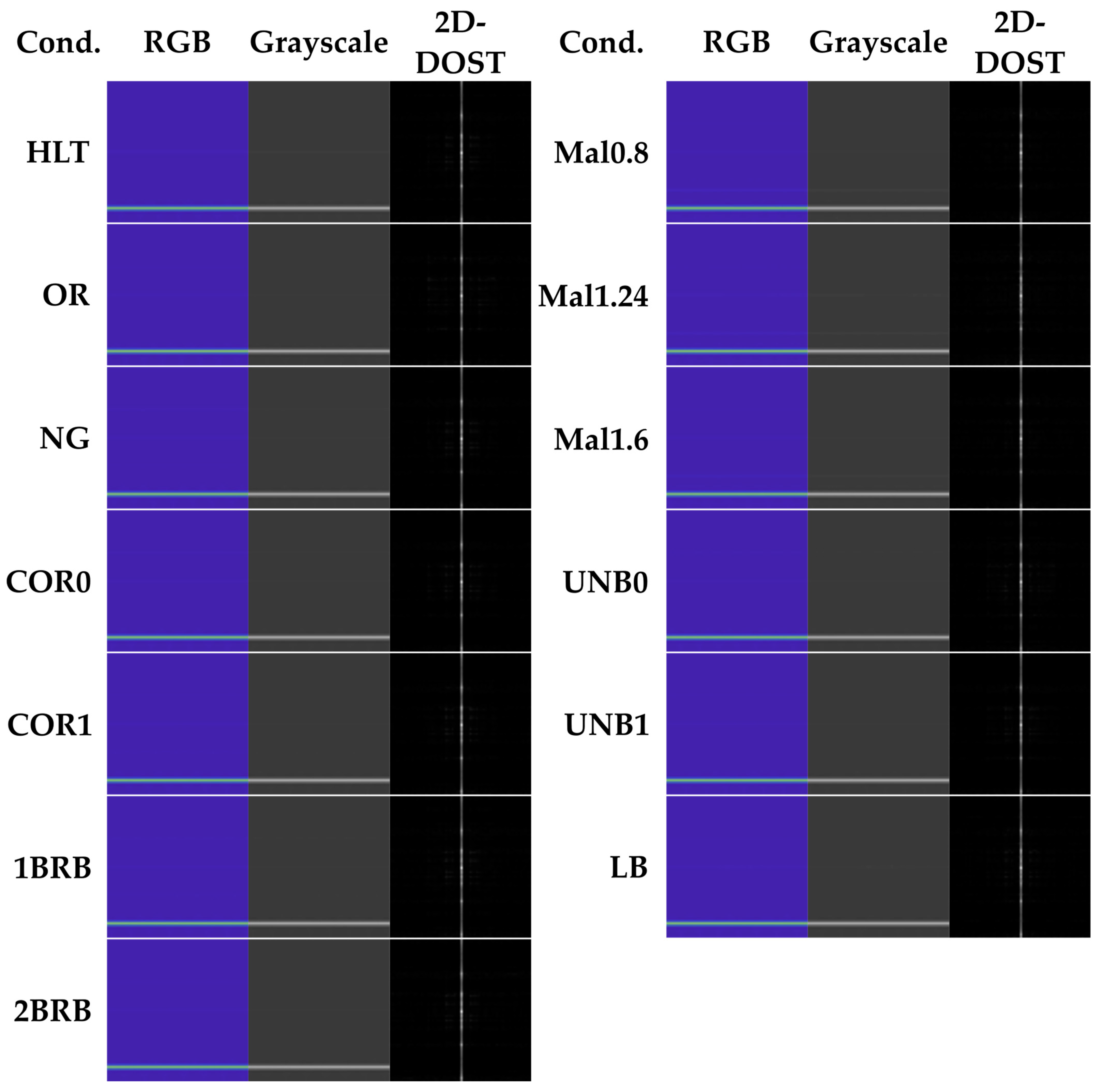
The grayscale figures were then processed using the 2D-DOST to obtain new representations, as this version of the DOST is used as a texture analysis tool in the image processing field, creating a different representation of the data in the pictures. In Figure 6, a comparison of the datasets is provided, having some elements in common and particularities regarding the information for each condition, making it harder to differentiate them.

From Figure 4, Figure 5 and Figure 6, it is possible to identify some variations in the data for the fault conditions regardless of the set of pictures; however, the subtlety of the changes in the spectrums makes it hard for the human eye to easily identify the conditions by looking for specific frequency components as performed in traditional approaches.

3.2. CNN Classification

As mentioned in the methodology, a lightweight CNN was used to classify the twelve conditions of the IM. For each set of images, ten training-testing-validation processes were carried out, obtaining parameters such as accuracy and training time to evaluate the impact of the 2D-DOST over the fault detection task. In

Table 3. CNN results for the classification of the STFT datasets.

Trial	RGB		Grayscale		2D-DOST
	Accuracy (%)	Time (s)	Accuracy (%)	Time (s)	Accuracy (%)	Time (s)
1	93.7388	77.7101	92.3076	81.5373	97.2271	80.8875
2	95.3041	77.7785	94.7227	78.9035	98.1216	81.7360
3	96.1091	77.6440	86.3148	79.2949	97.8980	81.4753
4	91.1896	83.5242	94.0966	80.4095	97.9874	79.4998
5	97.7191	87.5557	79.4722	79.8887	98.3899	79.1721
6	94.4096	79.9789	94.8568	81.5676	98.1216	80.6396
7	94.5438	76.3623	90.6976	81.8278	97.7638	81.5238
8	93.5599	76.3259	91.2343	79.6716	98.3899	83.0410
9	93.7388	78.9607	93.4257	79.4539	97.9874	80.9707
10	91.4132	83.6466	88.7745	80.1647	97.0930	79.2202
Average	94.1726	79.9487	90.5903	80.2719	97.8980	80.8166
Std. Deviation	1.9738	3.7464	4.7630	1.0400	0.4366	1.2371

, the accuracy and training time for the STFT sets are presented, and the best accuracy with the respective training time is highlighted for each set, as well as the best global performance. Additionally, the average time for the classification of one RGB picture was 0.001366 s, for grayscale images it was 0.001029 s, and for 2D-DOST-treated images it was 0.000980 s, meaning the proposed method allows for faster diagnostic decisions.

Considering that the 2D-DOST subset performed better on average,

Table 4. Average confusion matrix for the STFT + 2D-DOST dataset results.

		Predicted Class
		1BRB	2BRB	NG	OR	COR0	COR1	HLT	LB	Mal0.8	Mal1.6	Mal1.24	UNB0	UNB1
True class	1BRB	100	0	0	0	0	0	0	0	0	0	0	0	0
	2BRB	0	99.94	0	0	0.05	0	0	0	0	0	0	0	0
	NG	0	0	97.55	0	0.58	0	0.05	0.05	0	0	0	0	0
	OR	0	0	0	99.76	0.23	0	0	0	0	0.05	0	0	0
	COR0	0	0.05	1.27	0.23	98.13	0.23	0.05	0	0.11	0.05	0	0.11	0.98
	COR1	0	0	0	0	0.17	98.60	0.17	0.17	0.11	0	0.05	0.93	0.11
	HLT	0	0	0.58	0	0	0.23	97.26	4.36	0	0	0.05	0.17	0.05
	LB	0	0	0.11	0	0	0.17	1.62	94.70	0	0	0.17	0.23	0.05
	Mal0.8	0	0	0.23	0	0.17	0.29	0	0	97.03	1.68	0.05	0.29	0
	Mal1.6	0	0	0.05	0	0.11	0.05	0	0	2.38	97.79	0.46	0.05	0
	Mal1.24	0	0	0	0	0	0	0.23	0	0.17	0.34	99.01	0.34	0.05
	UNB0	0	0	0.11	0	0.11	0.40	0.46	0.63	0.17	0	0.11	95.98	1.86
	UNB1	0	0	0.05	0	0.40	0	0.11	0.05	0	0.05	0.05	1.86	96.86

shows the average confusion matrix for the set in percentage, presenting some difficulties in differentiating between related classes but achieving good results in most cases.

In

Table 5. CNN results for the classification of the CWT datasets.

Trial	RGB		Grayscale		2D-DOST
	Accuracy (%)	Time (s)	Accuracy (%)	Time (s)	Accuracy (%)	Time (s)
1	96.0196	79.4532	76.6547	72.3464	94.7227	79.1546
2	91.7262	78.8669	87.2987	72.6272	97.2271	83.1524
3	91.1896	78.6685	82.1556	72.9206	96.1538	79.6102
4	94.4991	92.3172	88.2826	81.1488	96.4222	72.4330
5	87.8801	92.8950	91.0107	82.9375	96.9141	72.4931
6	94.4096	84.2634	88.2379	84.1502	95.8855	73.7472
7	87.2540	79.1323	84.2576	74.5516	96.0196	84.9196
8	95.0805	78.5048	83.2737	72.4960	97.1377	86.5207
9	92.2629	86.1035	78.3989	72.8847	97.4955	85.8286
10	95.7960	85.8342	89.0429	72.7790	95.3935	86.4226
Average	92.6118	83.6039	84.8613	75.8842	96.3372	80.42826
Std. Deviation	3.1387	5.6166	4.7570	4.8257	0.8787	5.8082

, the accuracy and training time for the CWT sets are presented, and the best accuracy with the respective training time is highlighted for each set, as well as the best global performance. Additionally, the average time for the classification of one RGB picture was 0.000971 s, for grayscale images it was 0.000911 s, and for 2D-DOST-treated images it was 0.001025 s, meaning the proposed method presented a small increase in time relative to the other options.

Considering that the 2D-DOST subset performed the best,

Table 6. Average confusion matrix for the CWT + 2D-DOST dataset results.

		Predicted Class
		1BRB	2BRB	NG	OR	COR0	COR1	HLT	LB	Mal0.8	Mal1.6	Mal1.24	UNB0	UNB1
True class	1BRB	100	0	0	0	0	0	0	0	0	0	0	0	0
	2BRB	0	99.82	0	0	0	0	0	0	0	0	0	0	0
	NG	0	0	99.12	0	1.45	0	0.05	0	0	0	0.23	0.05	0
	OR	0	0	0	99.59	0.17	0	0	0	0	0	0	0.11	0.05
	COR0	0	0	0.52	0.23	97.67	0	0	0	0.11	0	0.11	0.11	0
	COR1	0	0	0	0	0	98.02	0.98	0.23	0.23	0.05	0	0.05	0
	HLT	0	0	0.05	0	0.05	1.22	98.60	0.98	0.34	0	0.34	0.17	0.05
	LB	0	0	0	0.11	0	0.40	0.29	97.20	0.40	0	0.29	1.45	0.46
	Mal0.8	0	0.05	0	0	0.29	0	0	0.11	92.61	1.04	0.93	0.23	0
	Mal1.6	0	0.11	0	0.05	0.29	0.34	0	0	5.63	98.83	0	0.05	0
	Mal1.24	0	0	0	0	0.05	0	0.05	0.11	0.63	0	96.62	0.63	0.63
	UNB0	0	0	0	0	0	0	0	0.75	0	0.05	0.40	80.63	5.17
	UNB1	0	0	0.29	0	0	0	0	0.58	0	0	1.04	16.45	93.60

shows the average confusion matrix for the set in percentage, demonstrating some difficulties in differentiating between classes but achieving good results in most cases, with the greater decrease in accuracy for the UNB0 condition.

Similarly,

Table 7. Classification results for the FSST datasets using the proposed CNN model.

Trial	RGB		Grayscale		2D-DOST
	Accuracy (%)	Time (s)	Accuracy (%)	Time (s)	Accuracy (%)	Time (s)
1	90.0268	77.2022	85.8228	79.0852	93.1574	81.5256
2	95.3041	77.0565	87.4329	79.1243	93.2021	80.8298
3	94.0071	76.8338	77.5491	79.6006	95.5724	78.9573
4	92.8890	83.9461	85.4651	80.8249	94.2754	79.9391
5	88.7745	84.0221	86.0912	81.2045	94.7674	79.9763
6	91.2343	82.7658	83.0500	80.7172	93.9177	81.1804
7	90.6529	86.1356	87.6118	79.3112	95.0357	81.7306
8	90.2951	88.7534	83.3631	79.4883	94.8121	79.9261
9	91.5026	88.0623	79.4275	79.6827	95.3488	79.2309
10	91.4132	89.7371	86.6726	79.4623	95.3935	79.6656
Average	91.6100	83.4515	84.2486	79.8501	94.5483	80.2962
Std. Deviation	1.9553	4.9538	3.4160	0.7681	0.8805	0.9619

shows the results obtained when using FSST images as a basis for the diagnosis, with the best results highlighted. In this case, slightly lower accuracy is observed for all cases. Likewise, the average time for the classification of one RGB picture was 0.001067 s, for grayscale images it was 0.000973 s, and for 2D-DOST-treated images it was 0.001009 s, showing not much variation in the times captured for the previous datasets.

Table 8. Average confusion matrix for the FSST + 2D-DOST dataset results.

		Predicted Class
		1BRB	2BRB	NG	OR	COR0	COR1	HLT	LB	Mal0.8	Mal1.6	Mal1.24	UNB0	UNB1
True class	1BRB	99.70	0	0	0	0.05	0	0	0	0	0	0	0	0
	2BRB	0.05	100	0	0	0	0	0	0	0	0	0	0	0
	NG	0	0	98.31	0	0.46	0	0.05	0.17	0	0	0	0	0
	OR	0	0	0.05	99.76	0.05	0	0	0.11	0	0.29	0	0	0
	COR0	0	0	0.52	0.05	97.67	0.29	0	0.29	0	0.05	0	0	0
	COR1	0.23	0	0.29	0	1.33	91.62	2.15	1.51	0.81	0.11	0	0.05	0.05
	HLT	0	0	0.29	0	0	4.47	87.20	6.16	0.52	0	0.23	0.58	0.81
	LB	0	0	0.34	0	0.11	1.62	7.38	90.63	0	0	0.05	0.34	0.81
	Mal0.8	0	0	0	0	0.17	1.04	0.29	0	95.93	2.90	0.05	0	0
	Mal1.6	0	0	0.05	0	0.11	0.46	0	0	2.44	96.62	0	0	0
	Mal1.24	0	0	0.11	0	0	0.11	0.52	0.11	0.17	0	97.79	1.39	1.56
	UNB0	0	0	0	0	0	0.17	1.86	0.40	0.11	0	0.05	84.01	6.91
	UNB1	0	0	0	0.17	0	0.17	0.52	0.58	0	0	1.80	13.60	89.82

presents the average confusion matrix obtained for the 2D-DOST group, as it performed better than the other two image representations for the FSST, but presented greater problems for detecting unbalance-related classes when compared to the previous cases.

Continuing with the results from the CNN,

Table 9. Results obtained for the classification of the ST-MUSIC datasets.

Trial	RGB		Grayscale		2D-DOST
	Accuracy (%)	Time (s)	Accuracy (%)	Time (s)	Accuracy (%)	Time (s)
1	97.1824	76.3554	96.0644	79.5906	96.8694	78.6683
2	94.3649	76.5565	87.6118	79.7319	97.2271	79.2518
3	96.4669	77.6019	96.2880	81.8063	98.2558	79.2189
4	96.7352	82.7508	92.3076	83.4750	98.2558	78.7418
5	96.9141	84.3698	94.4096	79.1740	98.3899	81.1456
6	94.9016	86.2908	92.9785	79.2368	97.4955	81.5223
7	93.6940	88.1319	95.3041	79.8537	97.4508	78.7249
8	97.6296	90.5253	95.7960	81.4939	97.1377	78.9051
9	93.6493	88.5596	93.3363	81.6451	97.4955	79.9405
10	96.1091	87.3727	93.7835	81.4463	97.1824	79.2119
Average	95.7647	83.8514	93.7880	80.7454	97.5760	79.5331
Std. Deviation	1.4843	5.3053	2.5678	1.4274	0.5357	1.0233

displays the accuracies and times achieved using the ST-MUSIC TFDs, with the best results highlighted. Contrary to the FSST case, this set performs better throughout the different data presentations. In a similar manner to the previous datasets, the average time for the classification of one RGB picture was 0.001128 s, for grayscale images it was 0.001006 s, and for 2D-DOST-treated images it was 0.001169 s.

Likewise, in

Table 10. Average confusion matrix for the ST-MUSIC + 2D-DOST dataset.

		Predicted Class
		1BRB	2BRB	NG	OR	COR0	COR1	HLT	LB	Mal0.8	Mal1.6	Mal1.24	UNB0	UNB1
True class	1BRB	99.88	0	0.11	0	0.05	0	0	0	0	0	0	0.05	0
	2BRB	0	100	0	0	0	0	0	0	0	0	0	0	0
	NG	0	0	99.01	0	0.05	0	0	0	0	0	0	0	0
	OR	0.11	0	0	99.94	0	0	0	0	0	0	0	0	0
	COR0	0	0	0.87	0.05	99.88	0	0	0	0	0	0	0	0
	COR1	0	0	0	0	0	99.53	0.29	0	0	0	0	0.05	0
	HLT	0	0	0	0	0	0.05	93.13	4.18	0.05	0	0.05	1.04	0
	LB	0	0	0	0	0	0.11	5.81	95.75	0	0	0	0.63	0
	Mal0.8	0	0	0	0	0	0	0.05	0	96.27	3.83	0	0.11	0.17
	Mal1.6	0	0	0	0	0	0.23	0	0	3.43	96.04	0.05	0	0.05
	Mal1.24	0	0	0	0	0	0	0.11	0	0.17	0.05	99.82	0.52	0.05
	UNB0	0	0	0	0	0	0	0.52	0.05	0.05	0.05	0.05	92.50	3.0
	UNB1	0	0	0	0	0	0.05	0.05	0	0	0	0	5.05	96.68

, the average confusion matrix for the 2D-DOST case is displayed, showing fewer mistakes in the classification of the conditions, as all conditions present over 92% of correct detections for all conditions compared to the previous cases.

3.3. Comparison to Current Signals

To validate the proposal, the methodology was implemented to current signals that were captured simultaneously using a Fluke i300 current clamp (Universitat Politècnica de València, Valencia, Spain) on a Yokogawa DL350 scopecorder (Universitat Politècnica de València, Valencia, Spain) at 10 ksps. The signals went under the same normalization process, with a digital subsampling to obtain the same amount of datapoints in the signals and be able to compare on a more direct level. As mentioned in the Introduction, current signals and STFT are one of the main approaches to fault diagnosis on IMs, so only this combination was chosen to validate the capabilities of the proposal to improve the accuracy of various fault diagnosis. Figure 7 presents a comparison of the STFT images generated from the current signals in RGB, grayscale and the 2D-DOST; due to the resolution of the images, it is difficult to identify differences between the conditions in the same dataset. Another clarification is that only one current signal was captured per test, having 1/3 of the total amount of stray flux data, meaning that for each condition, there are 287 images, divided as 60% for CNN training, 20% for validation and 20% for testing.

In

Table 11. CNN results for the classification of the STFT current datasets.

Trial	RGB		Grayscale		2D-DOST
	Accuracy (%)	Time (s)	Accuracy (%)	Time (s)	Accuracy (%)	Time (s)
1	89.3387	15.5791	48.5829	14.7528	86.2348	16.0464
2	84.8852	15.6223	60.3238	14.7659	87.8542	16.2337
3	89.6086	15.7197	49.6626	14.7095	84.2105	15.8785
4	87.3144	15.6820	45.6140	14.7609	90.9581	15.7902
5	75.5735	15.7733	48.9878	16.3323	84.3454	15.7465
6	87.9892	15.6644	69.5006	16.1231	87.4493	15.7199
7	85.4251	15.7251	46.1538	15.5825	89.7435	15.8214
8	86.7746	15.7734	73.9541	15.8983	86.5047	15.8224
9	88.9338	15.8678	32.9284	15.6482	87.1794	15.7987
10	87.3144	15.8764	27.5303	15.9653	87.9892	15.7368
Average	86.3157	15.7284	50.3238	15.4539	87.2469	15.8594
Std. Deviation	4.0835	0.0973	14.5032	0.6439	2.1130	0.1612

, the accuracy and training time for the STFT current sets are presented, and the best accuracy with the respective training time is highlighted for each set, as well as the best global performance. Additionally, the average time for the classification of one RGB picture was 0.000925 s, for grayscale images it was 0.000986 s, and for 2D-DOST-treated images it was 0.000915 s, which is consistent to the results in the previous subsection.

In this case, the 2D-DOST set allowed for a slight increment in accuracy when compared to the RGB set.

Table 12. Average confusion matrix for the STFT + 2D-DOST current dataset results.

		Predicted Class
		1BRB	2BRB	NG	OR	COR0	COR1	HLT	LB	Mal0.8	Mal1.6	Mal1.24	UNB0	UNB1
True class	1BRB	92.98	0.52	0.35	0	0	1.22	0	0	0	0	0	0	0
	2BRB	0	99.47	0	0	0	0	0	0	0	0	0	0	0
	NG	0.17	0	49.64	7.01	7.19	0.17	7.89	2.80	0	0	0	0	0.35
	OR	0.52	0	9.29	78.24	5.43	1.05	3.68	4.56	0	0	0	2.98	0.70
	COR0	0.17	0	17.01	6.66	71.75	0.35	10.70	2.80	0	0	0	0	0.87
	COR1	5.61	0	0.52	0.70	0	97.01	0	0.35	0.17	0	0	0	0
	HLT	0.17	0	20.70	4.91	13.68	0	77.01	2.98	0	0	0	0	0
	LB	0.17	0	1.57	0.70	1.57	0	0.17	77.71	0.17	0	0	0	2.10
	Mal0.8	0	0	0	0	0	0	0	0.17	98.24	0.70	0	0	0
	Mal1.6	0	0	0	0	0	0	0	0	1.40	99.29	0	0	0
	Mal1.24	0	0	0	0	0	0	0	0	0	0	100	0	0
	UNB0	0	0	0	1.05	0	0	0	0	0	0	0	96.84	0
	UNB1	0.17	0	0.87	0.70	0.35	0.17	0.52	8.59	0	0	0	0.17	95.96

shows the average confusion matrix for the 2D-DOST set in percentage, demonstrating a similar behavior to the stray flux tests, where a good general performance with some conditions presented a higher level of misclassifications is appreciated.

3.4. Comparison to Other Methods in the Literature

To further provide a comparison of the methodology proposed in this paper, in

Table 13. Comparison of different fault detection proposals.

Proposal	Technique	Classification Model	Number of Conditions	Fault Location	Signals	Accuracy
[9]	FSST	CNN	13	Bearing	Vibration	100%
[13]	STFT	Lightweight CNN	4	Bearing	Vibration	95.16%
[20]	CWT	dCNN	6	Bearing, rotor, stator	Vibration and current	99.83%
[22]	1D to 2D signal conversion	TL-dCNN	5	Bearing, rotor	Current	99.4%
Proposed method	STFT + 2D-DOST	Lightweight CNN	13	Bearing, rotor, coupling, carcass	Stray flux	97.89%
	CWT + 2D-DOST					96.33%
	FSST + 2D-DOST					94.54%
	ST-MUSIC + 2D-DOST					97.57%

, a comparison of the results achieved to the some in the literature for the detection of faults in IMs is provided, with the proposed method average accuracies around the expected level. As mentioned before, most works focus on faults located in one part or component of the machine or on one type of fault, with a limited number of conditions. Additionally, the focus of this article is to analyze the effect of using image processing tools as preprocessing steps to improve multiple fault classification while using non-invasive stray flux sensors.

4. Discussion

The graphs displayed in Figure 3 illustrate the differences between the TFDs chosen for this paper, as the content in each one represents the same information in a different way, like having a logarithmic distribution in the case of the CWT, more definition in the frequency components with the FSST in comparison to the STFT, or a richer distribution in the ST-MUSIC. The comparison in Figure 4 showed that the faults presented not enough information in the spectrograms to distinguish all conditions easily from one another in each dataset; the same could be said about the grayscale images in Figure 5, which presented less detail due to the color palette, making it more difficult to discriminate the conditions by eye. Similarly, the comparison in Figure 6 presented the same tendency, as most conditions share similar patterns with variations that are hard to identify.

The automatic feature extraction performed by the CNN was able to tackle this problem, achieving good results in most cases. As seen in Table 3, Table 5, Table 7 and Table 9, RGB images reached high results in condition classification in most cases while the use of grayscale pictures represented a reduction in the performance of the model, possibly related to the lower detailed and information, as those images have information of the three color layers (RGB) condensed in one; contrarily, the results when using the 2D-DOST processed datasets showed an improvement over the RGB sets, this could be caused by the distribution of the information performed by the DOST, which could facilitate the extraction of features performed by the CNN model.

Regarding the TFDs used, STFT, CWT and FSST have been used to detect faults in IMs, mostly in bearings, and have proved to be effective when discriminating against a couple of conditions affecting different components of the motor. On the other hand, the MUSIC algorithm is considered more resource-consuming, and the short-time variation is less common for fault detection; however, it showed a better performance on average and a similar average training time reduction as the other TFDs. All transforms showed adequate results for identifying the twelve conditions and presented similar difficulties when diagnosing the severities of misalignment and unbalance, as the literature says that both conditions present similar frequency components. The implementation of the 2D-DOST over the TFDs helped the classification task with minimal computational load; this could be of great benefit when the use of more established methods, like the ones compared in this work, do not reach optimal accuracy levels, improving the fault diagnosis, even when other techniques struggle to identify as many and diverse conditions as reported in this research.

The comparison to the current signal analysis employing the proposed methodology shows that the proposal is suitable for application on different signals as the performance achieved when using current signals with STFT images is similar to that of the stray flux and different TFDs, even with reduced data. The CNN model, significantly smaller than most of the extensively reported models in the literature, performed adequately in all cases, allowing for a good performance during the tests. The information displayed in Table 13 shows that the results obtained fall within the range presented in the literature, taking into account the amount of conditions under detection and the difference in size and parameters for all CNN models, as well as the validity of the approach, as a way to improve the classification performance by using a tool that facilitates the automatic feature extraction performed by a CNN model considerably smaller than some of the preferred nets, as mentioned in Section Experimental Setup.

5. Conclusions

This work focused on analyzing the effect of the 2D-DOST, an image processing tool used in the medical field as a texture analysis technique capable of improving condition diagnosis, on the fault detection in IMs. To contrast the influence of this technique, RGB and grayscale TFDs of the STFT, CWT, FSST, and ST-MUSIC were used as baselines, and their classification performance was compared to that of the TFDs after a 2D-DOST treatment. The results showed using RGB images achieved good accuracy, while grayscale pictures reduced the performance of the CNN model; in contrast, the results from the 2D-DOST batch improved the RGB results with minimal changes in computational load. The use of image processing tools on the inputs to CNN models could greatly benefit the condition monitoring and fault detection area, as they could facilitate the extraction of features, improving the overall accuracy and reducing the need for larger models that require more resources. This methodology showed good performance for identifying eleven faulty conditions of five different natures and various severities, proving that it could be applied to different scenarios. Additionally, the application of the method to TFDs of current signals generated using STFT showed similar results to the stray flux analysis, demonstrating the applicability of the proposal to other signals, even with a reduced number of samples.

Further research is necessary to understand the mechanisms that influence the performance of the TFDs when the 2D-DOST is used, as well as to compare whether the results extend to other transforms or 2D representations, or if similar image processing tools have similar effects. Prospective work includes the automation of the process to generate an online system that could identify the presence of faults on working machines to allow for early detection and corrective maintenance measures, reducing the impact of the faults, as well as expanding the results to consider early fault detection and progressive severity increments.

References

1. Gundewar, S.K.; Kane, P.V. Condition monitoring and fault diagnosis of induction motor. J. Vib. Eng. Technol. 2021, 9, 643–674. [Google Scholar] [CrossRef]
2. Kumar, R.R.; Andriollo, M.; Cirrincione, G.; Cirrincione, M.; Tortella, A. A Comprehensive Review of Conventional and Intelligence-Based Approaches for the Fault Diagnosis and Condition Monitoring of Induction Motors. Energies 2022, 15, 8938. [Google Scholar] [CrossRef]
3. Almounajjed, A.; Sahoo, A.K.; Kumar, M.K.; Assaf, T. Fault diagnosis and investigation techniques for induction motor. Int. J. Ambient Energy 2021, 43, 6341–6361. [Google Scholar] [CrossRef]
4. De Jesus Rangel-Magdaleno, J. Induction Machines Fault Detection: An Overview. IEEE Instrum. Meas. Mag. 2021, 24, 63–71. [Google Scholar] [CrossRef]
5. Zamudio-Ramirez, I.; Osornio-Rios, R.A.A.; Antonino-Daviu, J.A.; Razik, H.; De Jesus Romero-Troncoso, R. Magnetic Flux Analysis for the Condition Monitoring of Electric Machines: A Review. IEEE Trans. Ind. Inform. 2021, 18, 2895–2908. [Google Scholar] [CrossRef]
6. Abbasi, M.A.; Huang, S.; Khan, A.S. Fault detection and classification of motor bearings under multiple operating conditions. ISA Trans. 2024, 156, 61–69. [Google Scholar] [CrossRef]
7. Gundewar, S.K.; Kane, P.V. Bearing fault diagnosis using time segmented Fourier synchrosqueezed transform images and convolution neural network. Measurement 2022, 203, 111855. [Google Scholar] [CrossRef]
8. Wang, J.; Mo, Z.; Zhang, H.; Miao, Q. A Deep Learning Method for Bearing Fault Diagnosis Based on Time-Frequency Image. IEEE Access 2019, 7, 42373–42383. [Google Scholar] [CrossRef]
9. Łuczak, D. Data-Driven Machine Fault Diagnosis of Multisensor Vibration Data Using Synchrosqueezed Transform and Time-Frequency Image Recognition with Convolutional Neural Network. Electronics 2024, 13, 2411. [Google Scholar] [CrossRef]
10. Fu, M.; Du, D.; Leng, F.; Tian, J.; Fang, Y.; Zhang, J. Motor Bearing Fault Diagnosis Based on Fourier-based Synchrosqueezing Transform and Hilbert Envelope Spectrum. In Proceedings of the 2023 IEEE 6th Student Conference on Electric Machines and Systems (SCEMS), Huzhou, China, 7–9 December 2023; pp. 1–6. [Google Scholar] [CrossRef]
11. Rajabioun, R.; Afshar, M.; Mete, M.; Atan, Ö.; Akin, B. Distributed Bearing Fault Classification of Induction Motors Using 2-D Deep Learning Model. IEEE J. Emerg. Sel. Top. Ind. Electron. 2023, 5, 115–125. [Google Scholar] [CrossRef]
12. Mitra, S.; Koley, C. Real-time robust bearing fault detection using scattergram-driven hybrid CNN-SVM. Electr. Eng. 2023, 106, 3615–3625. [Google Scholar] [CrossRef]
13. Irgat, E.; Çinar, E.; Ünsal, A.; Yazıcı, A. An IoT-Based Monitoring System for Induction Motor Faults Utilizing Deep Learning Models. J. Vib. Eng. Technol. 2022, 11, 3579–3589. [Google Scholar] [CrossRef]
14. Bouharrouti, N.E.; Saberi, A.N.; Khan, M.D.H.; Kudelina, K.; Naseer, M.U.; Belahcen, A. Deep Transfer Learning Approach Using Filtered Time-Frequency Representations of Current Signals for Bearing Fault Detection in Induction Machines. IET Electr. Power Appl. 2025, 19. [Google Scholar] [CrossRef]
15. Qi, J.; Chen, Z.; Kong, Y.; Qin, W.; Qin, Y. Attention-guided graph isomorphism learning: A multi-task framework for fault diagnosis and remaining useful life prediction. Reliab. Eng. Syst. Saf. 2025, 263, 111209. [Google Scholar] [CrossRef]
16. Valtierra-Rodriguez, M.; Rivera-Guillen, J.R.; Basurto-Hurtado, J.A.; De-Santiago-Perez, J.J.; Granados-Lieberman, D.; Amezquita-Sanchez, J.P. Convolutional Neural Network and Motor Current Signature Analysis during the Transient State for Detection of Broken Rotor Bars in Induction Motors. Sensors 2020, 20, 3721. [Google Scholar] [CrossRef] [PubMed]
17. Misra, S.; Kumar, S.; Sayyad, S.; Bongale, A.; Jadhav, P.; Kotecha, K.; Abraham, A.; Gabralla, L.A. Fault Detection in Induction Motor Using Time Domain and Spectral Imaging-Based Transfer Learning Approach on Vibration Data. Sensors 2022, 22, 8210. [Google Scholar] [CrossRef] [PubMed]
18. Zamudio-Ramirez, I.; Osornio-Rios, R.A.; Antonino-Daviu, J. Transient stray flux analysis via music methods for the detection of uniform gearbox teeth wear faults. In Proceedings of the 2021 IEEE Energy Conversion Congress and Exposition (ECCE), Vancouver, BC, Canada, 10–14 October 2021; pp. 4431–4435. [Google Scholar] [CrossRef]
19. Biot-Monterde, V.; Navarro-Navarro, A.; Zamudio-Ramirez, I.; Antonino-Daviu, J.A.; Osornio-Rios, R.A. Automatic classification of eccentricities and misalignments in SCIM applying persistence spectrum and CNN to stray-flux signals. In Proceedings of the 2023 IEEE Energy Conversion Congress and Exposition (ECCE), Nashville, TN, USA, 29 October–2 November 2023; pp. 4057–4061. [Google Scholar] [CrossRef]
20. Shao, S.; Yan, R.; Lu, Y.; Wang, P.; Gao, R.X. DCNN-Based Multi-Signal Induction Motor Fault Diagnosis. IEEE Trans. Instrum. Meas. 2019, 69, 2658–2669. [Google Scholar] [CrossRef]
21. Delgado-Arredondo, P.A.; Garcia-Perez, A.; Morinigo-Sotelo, D.; Osornio-Rios, R.A.; Avina-Cervantes, J.G.; Rostro-Gonzalez, H.; Romero-Troncoso, R.D. Comparative Study of Time-Frequency Decomposition Techniques for Fault Detection in Induction Motors Using Vibration Analysis during Startup Transient. Shock. Vib. 2015, 2015, 708034. [Google Scholar] [CrossRef]
22. Kumar, P.; Hati, A.S. Transfer learning-based deep CNN model for multiple faults detection in SCIM. Neural Comput. Appl. 2021, 33, 15851–15862. [Google Scholar] [CrossRef]
23. Drabycz, S.; Stockwell, R.G.; Mitchell, J.R. Image texture characterization using the discrete orthonormal S-transform. J. Digit. Imaging 2009, 22, 696–708. [Google Scholar] [CrossRef]
24. Soleimani, M.; Vahidi, A.; Vaseghi, B. Two-Dimensional Stockwell Transform and Deep Convolutional Neural Network for Multi-Class Diagnosis of Pathological Brain. IEEE Trans. Neural Syst. Rehabil. Eng. 2020, 29, 163–172. [Google Scholar] [CrossRef]
25. Pridham, G.; Oladosu, O.; Zhang, Y. Evaluation of discrete orthogonal versus polar Stockwell Transform for local multi-resolution texture analysis using brain MRI of multiple sclerosis patients. Magn. Reson. Imaging 2020, 72, 150–158. [Google Scholar] [CrossRef] [PubMed]
26. Asgharzadeh-Bonab, A.; Kalbkhani, H.; Azarfardian, S. An Alzheimer’s disease classification method using fusion of features from brain Magnetic Resonance Image transforms and deep convolutional networks. Healthc. Anal. 2023, 4, 100223. [Google Scholar] [CrossRef]
27. Saghazadeh, A.; Rezaei, N. Artificial Intelligence: A Tool to Help Cancer Diagnosis, Prognosis, and Treatment. In Handbook of Cancer and Immunology; Springer International Publishing: Cham, Switzerland, 2023; pp. 1–29. [Google Scholar] [CrossRef]
28. Alhasan, A.S. Clinical Applications of Artificial Intelligence, Machine Learning, and Deep Learning in the Imaging of Gliomas: A Systematic Review. Cureus 2021, 14, 13. [Google Scholar] [CrossRef] [PubMed]
29. Nayak, G.; Padhy, N.; Mishra, T.K. 2D-DOST for seizure identification from brain MRI during pregnancy using KRVFL. Health Technol. 2022, 12, 757–764. [Google Scholar] [CrossRef]
30. Díaz-Saldaña, G.; Morales-Velásquez, L.; Antonio-Daviu, J.A.; Biot-Monterde, V. Comparison of Bearing Fault Classification Using STFT, CWT and 2D-DOST with a Lightweight CNN Model. In Proceedings of the 2025 IEEE 34th International Symposium on Industrial Electronics (ISIE), Toronto, ON, Canada, 20–23 June 2025; pp. 1–6. [Google Scholar] [CrossRef]
31. Guerrero, J.P.P.; Saucedo-Dorantes, J.J.; Osornio-Rios, R.A.; Antonino-Daviu, J.A.; Biot-Monterde, V. Unbalance and misalignment detection in induction motors under oscillating loads using current and Fast Fourier Transform (FFT). In Proceedings of the 2023 IEEE Energy Conversion Congress and Exposition (ECCE), Nashville, TN, USA, 29 October–2 November 2023; pp. 4202–4207. [Google Scholar] [CrossRef]
32. Yu, F.T.S.; Lu, G. Short-time Fourier transform and wavelet transform with Fourier-domain processing. Appl. Opt. 1994, 33, 5262. [Google Scholar] [CrossRef]
33. Özhan, O. Short-Time-Fourier Transform. In Basic Transforms for Electrical Engineering; Springer: Cham, Switzerland, 2022. [Google Scholar] [CrossRef]
34. Sadowsky, J. The continuous wavelet transform: A tool for signal investigation and understanding. Johns Hopkins APL Tech. Dig. 1994, 15, 306. [Google Scholar]
35. Oberlin, T.; Meignen, S.; Perrier, V. The Fourier-based synchrosqueezing transform. In Proceedings of the 2014 IEEE international conference on acoustics, speech and signal processing (ICASSP), Florence, Italy, 4–9 May 2014; pp. 315–319. [Google Scholar] [CrossRef]
36. Chen, Z.; Ji, Y.; Zhang, Y.; Tang, F.; Dong, Z. Ionosphere Phase Decontamination for OTHR Based on Fourier Synchrosqueezed Transform. In Proceedings of the 2024 IEEE International Conference on Signal, Information and Data Processing (ICSIDP), Zhuhai, China, 22–24 November 2024; pp. 1–5. [Google Scholar] [CrossRef]
37. Chavez, O.; Amezquita-Sanchez, J.P.; Valtierra-Rodriguez, M.; Cruz-Abeyro, J.A.; Kotsarenko, A.; Millan-Almaraz, J.R.; Dominguez-Gonzalez, A.; Rojas, E. Novel ST-MUSIC-based spectral analysis for detection of ULF geomagnetic signals anomalies associated with seismic events in Mexico. Geomat. Nat. Hazards Risk 2015, 7, 1162–1174. [Google Scholar] [CrossRef][Green Version]
38. Stockwell, R.G.; Mansinha, L.; Lowe, R.P. Localization of the complex spectrum: The S transform. IEEE Trans. Signal Process. 2002, 44, 998–1001. [Google Scholar] [CrossRef]
39. Battisti, U.; Riba, L. Window-dependent bases for efficient representations of the Stockwell transform. Appl. Comput. Harmon. Anal. 2015, 40, 292–320. [Google Scholar] [CrossRef]
40. Li, B. Lightweight Neural Networks. In Embedded Artificial Intelligence; Springer: Singapore, 2024. [Google Scholar] [CrossRef]
Figure 1. Block diagram illustrating the methodology followed in this research.
Machines 13 01001 g001
Figure 2. Experimental setup: (a) IM, load and location of the stray flux sensor; (b) commercial tool for alignment measuring the misalignment; (c) rotor with one BRB; (d) bearing with corrosion condition, COR1; (e) coupling and weight used for the UNB1 condition.
Machines 13 01001 g002
Figure 3. Samples of the TFDs used for a HLT sample: (a) STFT; (b) CWT; (c) FSST; (d) ST-MUSIC.
Machines 13 01001 g003aMachines 13 01001 g003b
Figure 4. Comparison of the RGB images for all conditions and TFDs.
Machines 13 01001 g004
Figure 5. Comparison of the grayscale datasets for all TFDs.
Machines 13 01001 g005
Figure 6. Comparison of the TFDs for all conditions after the 2D-DOST processing.
Machines 13 01001 g006
Figure 7. Comparison of the images generated from the current signals for all conditions and TFDs.
Machines 13 01001 g007