Abstract
Finite element (FE) models are widely used in structural health monitoring to represent real structures and assess their condition, but discrepancies often arise between numerical and actual structural behavior due to simplifying assumptions, uncertain parameters, and environmental influences. Temperature variation, in particular, significantly affects structural stiffness and modal properties, yet it is often treated as noise in traditional model updating methods. This study treats temperature changes as valuable information for model updating and structural damage quantification. The Bayesian model updating approach (BMUA) is a probabilistic approach that updates uncertain model parameters by combining prior knowledge with measured data to estimate their posterior probability distributions. However, traditional BMUA methods assume mass is known and only update stiffness. A novel BMUA framework is proposed that incorporates thermal buckling and temperature-dependent stiffness estimation and introduces an algorithm to eliminate the coupling effect between mass and stiffness by using temperature-induced stiffness changes. This enables the simultaneous updating of both parameters. The framework is validated through numerical simulations on a three-story aluminum shear frame under uniform and non-uniform temperature distributions. Under healthy and uniform temperature conditions, stiffness parameters were estimated with high accuracy, with errors below 0.5% and within uncertainty bounds, while mass parameters exhibited errors up to 13.8% that exceeded their extremely low standard deviations, indicating potential model bias. Under non-uniform temperature distributions, accuracy declined, particularly for localized damage cases, with significant deviations in both parameters.
1. Introduction
Finite element models (FEMs) are employed in civil and structural engineering for system response and control [1,2], structural health monitoring (SHM) [3,4,5,6,7], or reliability and risk assessment [8,9]. Discrepancies between FE models and physical structures always exist. The sources of discrepancies mainly result from (1) modeling errors from the ideal assumption in FE modal construction, (2) statistical uncertainties in material and geometric properties, and (3) irregularities in structure [4,10,11]. These issues may impair the quality and accuracy of numerical models. Therefore, FE model updating (FEMU) techniques are developed to calibrate and identify parameters for minimizing the gap between FE model predicted and measured vibrational data [12,13,14]. Iterative methods, particularly stochastic and deterministic approaches, are widely used for FEMU, offering robust solutions for updating complex structural models [10,15]. The deterministic approach seeks to determine the optimal parameter of the numerical model, thereby achieving the best fit between the model’s output and the measured data. However, model updating is inherently an inverse problem, making it sensitive to measurement noise, incomplete data, and modeling errors. These issues often lead to uncertainties and ill-posed problems, limiting the model’s robustness. A stochastic approach is essential to address these challenges effectively. Incorporating uncertainty quantification allows for the assessment of the impact of uncertainties on model parameters and predictions, improving the decision-making process regarding the maintenance, repair, or replacement of structural components [11,12].
The Bayesian model updating approach (BMUA) is an advanced FEMU technique to update structural parameters using modal data and account for underlying uncertainties [13,14,16]. This method has achieved satisfactory practical real-world application in recent years in buildings [17,18] and bridges [19]. This method treats model parameters as random variables, and they are identified by their most probable values (MPVs). The posterior probability density function (PDF) associated with these parameters naturally represents their uncertainty, providing a robust framework to characterize parameter uncertainty.
However, traditional Bayesian methods typically assume that structural properties remain constant over time, with uncertainties attributed solely to measurement noise [20]. Additionally, the traditional BMUA assumes that mass is known and only updates stiffness to prevent the coupling effect of mass and stiffness, as discussed in Section 2.1 of this study. But the assumption fails if there is also a loss in mass due to damage or mistakes in determining mass from the engineering drawing. There are a few works that address this problem by updating mass and stiffness with uncertainty quantification [21,22,23], but the temperature effect is not considered.
1.1. Problem Statement and Motivation
Although vibration-based structural condition assessment has been widely used over the last decade, a successful condition assessment relies heavily on the accuracy of the measured vibrational properties, such as the natural frequencies and mode shapes of structures. However, a major challenge arises from the fact that these vibration properties are influenced by environmental factors, such as temperature, traffic, wind, and humidity [20]. Research has shown that temperature-induced vibration variation can be greater than that resulting from moderate structural damage or typical operational load [24].
Numerous studies have been conducted to investigate the temperature effect on modal frequencies. For an experiment performed on the Alamosa Canyon Bridge, it was found that the first mode frequency varied by approximately 5% during a 24 h time period due to temperature effects [25]. Similarly, for a reinforced concrete span bridge monitored continuously for three years, a 10% seasonal change in natural frequency was observed due to the temperature variation [26]. The variation in temperature from −20 °C to 25 °C in the Confederation Bridge led to a reduction in modal frequency by 4% [27]. During the study of the two-span steel-concrete composite bridge for 24 h, the frequencies in all modes changed “1–2% daily” (from noon to night) [28]. Thus, it has been widely observed that there is a negative correlation between temperature and modal frequencies. So if there is no effort to include the temperature parameter in the updating process, there might be false detection of damage.
If the impact of environmental factors on changes in dynamic structural properties is not adequately accounted for, vibration-based damage detection techniques can generate inaccurate results, such as false positives or false negatives in identifying structural damage. So it is essential to model and account for the modal variability caused by temperature in vibration-based damage detection.
Zeng and Kim [29] introduced a novel BMUA to address the coupling effect between mass and stiffness by measuring two states of a structure: the original state and a modified state. The key idea is to formulate a new eigen equation for the modified system, which helps decouple the mass and stiffness parameters during the updating process. However, the practicality of this approach is limited because it relies on creating a modified system by retrofitting the structure model with added stiffness or by adding mass [30], which may not always be feasible or cost-effective in real-world applications. Also, the temperature effect on the structure was not considered [31,32].
1.2. Research Goal and Significance
The primary objective of this work is to develop an FEMU method that accounts for the temperature effect while eliminating the coupling effects of mass and stiffness. This method considers that the stiffness will change with temperature. By using modal data at the normal temperature and at different temperatures, we can decouple the mass and stiffness in the model updating process. To achieve the goal, the following tasks are identified:
- Create an algorithm to eliminate the coupling effect of mass and stiffness using the stiffness change caused by temperature variation.
- Validate the proposed algorithm in two scenarios: uniform and non-uniform temperature of the structure.
- Evaluate the probabilistic damage severity in structural parameters in both mass and stiffness.
To address research on temperature variations, a fundamental approach is essential. For this reason, a typical structure—specifically, a shear building model—is used to evaluate the proposed algorithms. Researchers commonly use shear building models as lab-scale experimental setups to test algorithms [33]. Usually, algorithms are first developed using simple models and then examined on more complex structures, such as bridges [34,35]. Therefore, applying these algorithms to other structural types, along with experimental testing, can be considered a direction for future research.
2. Proposed Approach
2.1. Fundamentals and Integrated Algorithm
Bayesian inference is a method of statistical inference in which Bayes’ theorem is used to calculate the probability of a hypothesis given prior evidence and update it as more information becomes available. In essence, Bayesian inference estimates posterior probabilities based on a prior distribution, because there are many modeling and parametric uncertainty issues in civil engineering problems, such as time-varying temperature, wind, ground motion, etc. Bayesian statistics is a crucial technique in civil engineering applications. In addition, it can be challenging to pinpoint the exact properties of materials such as concrete, as these materials’ varying production and construction are also uncertain. Moreover, joints are assumed to be fixed in place during modeling, but in practice, the boundary condition is affected by environmental conditions [36].
Traditional BMUA is generally considered an acceptable model updating tool; it primarily focuses on updating stiffness and is typically formulated using the classical eigenvalue equation as follows:
where and are the system stiffness and mass matrix, respectively, the eigenvalue corresponds to the square of the natural frequency, , and the eigenvector represents the corresponding mode shape. As we can see from Equation (1), and are coupled; that is, we need information on both system stiffness and mass stiffness to update, and there can be an infinite combination of mass and stiffness generating the same frequency. This makes it difficult to uniquely determine both parameters simultaneously [37].
To address this issue, it is often assumed that the mass remains constant or is accurately known from engineering drawings and material dimensions and properties, allowing only the stiffness to be updated. This assumption is made in the belief that mass variation has a minimal impact. However, if the structure is huge and undergoes some damage, such as spalling, there can be a considerable loss of mass that affects the dynamics of the structure. Therefore, relying on a fixed mass value can lead to incorrect stiffness estimations and inaccurate system predictions.
In this research, a BMUA is proposed to simultaneously update mass and stiffness while inherently addressing their coupling effect based on an earlier study [29]. Unlike previous methods that rely on physical modifications (e.g., mass or stiffness addition) to create a modified system, this approach leverages temperature changes to induce measurable variations in the structural response. This method eliminates the need for impractical retrofitting and incorporates environmental effects, such as temperature, into the updating process.
2.2. Change in Stiffness Due to Temperature
A structure subjected to heating effects from the sun or the environment can be described in terms of its distributed mass, damping, and stiffness matrices in the time domain via the following equation [38]:
where is the mass matrix, is the damping matrix, is the stiffness matrix, is the displacement vector, is the velocity vector, is the acceleration vector, and is the external force vector, but for the free vibration case .
For this study, the structure is assumed to be undamped so that only the degradation of material performance and thermal stress are taken into account, which affect the stiffness matrix due to temperature changes. The elastic stiffness matrix, , is affected by temperature-induced changes in elastic modulus, E. For simplicity in this study, a linear equation between temperature and aluminum elastic modulus is adopted, which is given by
where is the elastic modulus of the material at reference temperature, and is the thermal coefficient of the elastic modulus of the material.
When a compressive axial force is present in a member, the bending stiffness of the member is reduced. The stiffness matrix that reflects this kind of stress-stiffening effect is called the geometric stiffness matrix () [39]. Here, the element axial force is due to the longitudinal load, , caused by temperature in degrees Celsius, is the temperature coefficient of the elastic modulus, and is the elastic modulus of aluminum at 20 °C.
The elastic stiffness matrix for the i-th frame element is expressed as
where E, I, A, and L denote the elastic modulus, moment of inertia, cross-sectional area, and elemental length; the geometric stiffness matrix for the i-th frame element is expressed as
Hence, the equation of motion for an undamped free response structure is given by
For an undamped system, , the eigenvalue equation for the mode is given by
where is the natural frequency and is the corresponding mode shape. For this study, the standard temperature is assumed to be when the elements are free from all thermal stress. Note that in , the geometric stiffness matrix is zero.
Traditional FEMU is performed by identifying mass and stiffness matrices without considering temperature; however, in this study, an FE model updates the system stiffness matrices that change due to temperature. So, using the measured data, the correct mass and stiffness matrices can be determined using the correct mass and stiffness parameters and appropriate boundary conditions under different temperatures.
For simplicity, the heat transfer process in this study is neglected. Future work should aim to incorporate a more realistic thermal heat transfer process to better capture the coupled thermo-mechanical behavior of the structure.
2.3. Bayesian Model Updating Approach with Change in Temperature
Two systems—one at a reference temperature, , and another at a different temperature, T—exhibit changes in stiffness. At , the stiffness matrix is denoted by . At temperature T, the stiffness matrix becomes , which can be expressed as . Here, , where represents the change in elastic stiffness due to temperature variation. The derivation of the BMUA algorithm and uncertainty quantification is taken from [29,36,40].
2.4. Thermal Model of the Column
This study examines a simply supported Euler–Bernoulli beam with a rectangular cross-section, functioning as a column, as shown in Figure 1. The column consists of a linear elastic, isotropic, and homogeneous material, with dimensions of length l, width b, and thickness h along the x, y, and z axes, respectively. To simplify the model, the temperature distribution for a single element or column is uniform. The reference temperature denotes the stress-free state of the column in the absence of thermal effects.
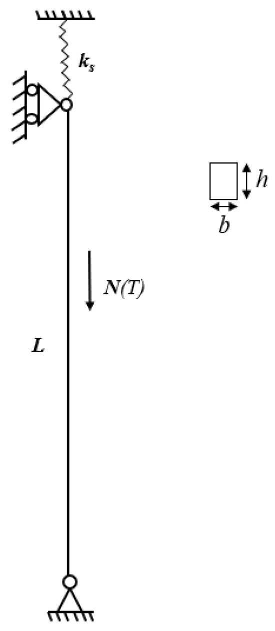
Figure 1.
A simply supported column with an axially movable boundary.
As discussed in the earlier Section 2.2, the temperature affects due to a change in the elasticity property of the material, as shown in Equation (3). The calculation of depends on the axial force , which is shown in Equation (6). In a conventionally supported column, both ends are restrained against certain translations and rotations, which restricts thermal expansion and significantly lowers the thermal buckling temperature [38]. As shown in Figure 1, axial translation is free but restrained by spring stiffness. The thermal buckling temperature is the critical temperature at which a structural element (like a beam, plate, or shell) becomes unstable due to thermal expansion under constraint [41]. An axial spring can be incorporated at the boundary so that the buckling temperature of the column is increased, as illustrated in Figure 1. For this study, the stiffness of the spring is calculated based on the additional stiffness required to reach the critical buckling temperature of the column at 100 °C. The calculation of spring stiffness is shown in Appendix A of this study, which is dependent on the length of the element. Then, the value of the spring is used to calculate the axial force due to temperature, as shown in Equation (6).
The axial thermal force on the column is given by [38]:
where the subscript for each parameter, , is the difference between and T, is the stiffness of the spring (N/m), L is the length of the column (m), E is the elastic modulus of the material (), A is the cross-sectional area of the member (), and is the linear expansion of the material (°C−1) at °C; however, A and are assumed to be constant in this study because the section dimensions are minimal.
The axial thermal force acts by compression, as the thermal expansion of the column is restrained by the boundary conditions. This restriction induces a compressive axial force that increases with temperature.
The procedure is summarized in Figure 2 and detailed step-by-step in Table 1. First, the spring stiffness required to increase the column’s thermal-buckling threshold is estimated. Then, the corresponding axial thermal load is computed from Equation (6), after which the temperature-induced stiffness change is calculated. Initial values for the mass and stiffness parameters are selected, after which the mode shapes corresponding to the m-th mode— and —are updated accordingly using the equations shown in Table 1. These updated shapes are used to recalculate the eigenvalues and via Steps 6a and 6b, respectively (see Table 1). The mass parameter and the stiffness-adjustment parameter are then updated. The sequence is iterated until the relative change in both and between successive iterations falls below , thereby satisfying the convergence criterion. The measurement of modal properties is simulated by adding small Gaussian noise to the true natural frequencies and mode shapes obtained from the finite element model. A coefficient of variation (C.O.V.) of 0.1% is used to mimic realistic measurement noise.
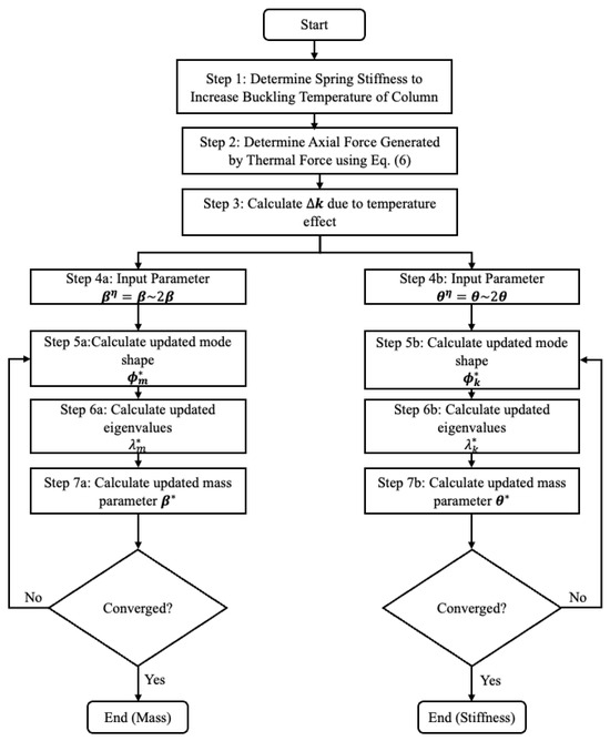
Figure 2.
Flowchart showing the updating procedure.

Table 1.
Summary of equations used in the Bayesian updating process.
Table 1 presents equations from the literature [29,36], where a BMUA is performed by physically modifying the structure to change its stiffness. In contrast, the updating approach proposed in this study uses stiffness changes caused by temperature variations, without any physical alteration to the structure. Importantly, the same equations can be applied here, as the change in stiffness is due to temperature effects rather than structural modification.
3. Description of the Structure
In this study, we followed the approach of previous works [29,36] and primarily considered a shear frame, focusing on lateral stiffness, to demonstrate the proposed procedure. An aluminum shear frame is used and subjected to both uniform and non-uniform thermal distributions. Here, the temperature of the column is increased to the temperature T from .
In a similar study, the spring was attached to increase the buckling temperature of the beam [38,42]. However, for this study, the column is modeled to increase the buckling load due to temperature. It is assumed that the critical buckling temperature of the column is , and the stiffness of the spring required to reach that temperature for buckling is estimated. The spring is also temperature-dependent. The elastic coefficient of the spring is taken as a linear function of temperature increase , shown by
where is the spring constant, which is estimated based on the stiffness required to increase the buckling temperature to 100 °C, and is the slope factor of the aluminum spring associated with temperature increase, which is taken as [38].
A three-story shear frame structure adopted from prior research [43], as shown in Figure 3, constructed entirely of aluminum, is used as the analytical model for this study. The base of the structure is fully restrained (fixed) to simulate realistic boundary conditions. Each floor slab has a square geometry measuring 0.3 m in width and 0.025 m in thickness.
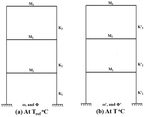
Figure 3.
Three-story shear building at uniform temperature.
The structural system is supported by four aluminum columns at each story level. The columns have a uniform height of 750 mm, a width of 2.5 mm, and a thickness of 0.6 mm. Furthermore, mass density, Young’s modulus, the coefficient of thermal expansion of the beam material, and the thermal coefficient of elastic modulus at the reference temperature are 2700, 69 GPa, , and 3.6 [38], respectively.
4. Results
The natural frequencies of the structure at various temperatures were determined through MATLAB (Version 25.1), which is used as finite element software for this study, and the results are summarized in Table 2. The data indicate that the frequencies for the first three modes decrease with increasing temperature, which is consistent with trends reported in the literature [25,26,27,28]. Two structural scenarios are considered in the updating process: one with a uniform temperature distribution and the other with a non-uniform distribution. Additionally, two damage cases are analyzed to evaluate the effectiveness of the proposed approach.
Table 2.
Natural frequencies (Hz) at different temperatures.
4.1. Considering Uniform Temperature
The proposed updating method, illustrated in Figure 2, was implemented by considering two distinct states: one at the reference temperature and the other at a uniform temperature of 50 °C applied across the entire structure. This uniform thermal condition was selected to reflect the state of the structure during the measurement. The values of mass and stiffness parameters for each floor are taken as 2, which is overestimated by 100%.
As shown in Table 3, the ‘Target’ column represents the actual stiffness and mass parameter as a target value in updating. The ‘Identified’ column represents the identified stiffness and mass parameters as the outcomes of the proposed approach. The standard deviation (s.d.) indicates the uncertainty of updating parameters, which is determined from covariance matrices in Equations (A49) and (A53). The identified stiffness parameters (, , ) show excellent agreement with their target values (all set to 1.0000), with low standard deviations and coefficients of variation, indicating high confidence in the estimates. However, the identified mass parameters (, , ), while numerically close to the targets, fall outside the uncertainty bounds and, thus, lie outside the confidence interval.
Table 3.
Updated stiffness and mass parameters (healthy condition).
Although the initial value of the parameters was set to 2, the optimization process rapidly guided them toward their target values. As shown in Figure 4 and Figure 5, all parameter values quickly converged and stabilized near 1 within the early iterations, demonstrating the effectiveness and stability of the updating procedure.
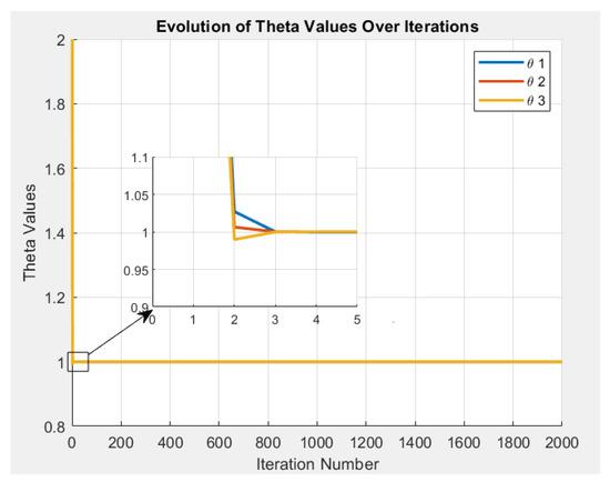
Figure 4.
Evolution of values over iterations.
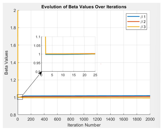
Figure 5.
Evolution of values over iterations.
Table 4 shows the frequency comparison between the measured natural frequency at the reference temperature, 20 °C, and at 50 °C, which is simulated by adding a zero-mean Gaussian noise with 0.1% C.O.V. and the updated natural frequency. The updated frequencies are compared with the target or measured at the reference temperature (20 °C) case; it can be observed that the error between them is less than 0.1%.
Table 4.
Modal frequency (Hz) comparison of measured and updated.
The modal assurance criterion (MAC) is used to evaluate how well the updated mode shapes align with the experimentally measured ones, to validate the accuracy of model updating. Figure 6 illustrates the MAC [44] comparison between the target/measured and updated mode shapes. The MAC values, ranging from 0 to 1, are used to quantify the degree of correlation between corresponding mode shapes obtained from experimental measurements, which are simulated, and those predicted by numerical models. A value close to 1 indicates a strong agreement between the two mode shapes, while values significantly less than 0.9 suggest discrepancies. The diagonal bars exhibit values of 1, indicating that the updated model closely matches the measured mode shapes for the corresponding modes. Off-diagonal elements display zero, confirming that each mode shape is most strongly correlated with its corresponding mode and not with others, thus validating the accuracy and orthogonality of the mode shapes.
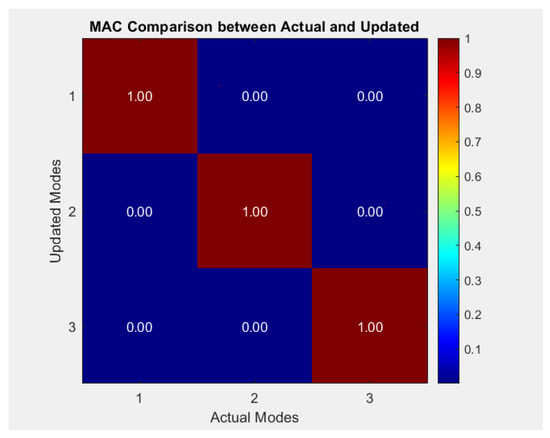
Figure 6.
Comparison of MAC between measured/target and updated modes.
Damage is created artificially by changing critical structural parameters such as flexure stiffness () and a change in the density of material. The negative sign represents the mass/stiffness loss with respect to undamaged values. The initial parameter for both mass and stiffness is taken as 1, as damage detection is usually conducted without prior information. Table 5 presents two damage scenarios (D1 and D2) characterized by specific changes in mass and stiffness at different floor levels of the shear frame. A low standard deviation in the estimated parameters—such as mass or stiffness—indicates that the data points are clustered closely around the mean, which is assumed to represent the degree of damage. Therefore, the exact magnitude of the estimated damage may not be critical at certain damage levels. Further parametric studies are needed to confirm the effectiveness of this damage detection approach in both experimental and simulation settings.
Table 5.
Damage cases with mass and stiffness changes.
Table 6 presents a comparison between the target and identified values of the stiffness and mass parameters for Damage Case 1. As shown in the table, the identified stiffness parameters closely match the target values, with a maximum error of only 0.41%. However, the identified mass parameters ( and ) deviate from their corresponding target values, with a maximum error of 11% and lying outside the confidence interval.
Table 6.
Updated stiffness and mass parameters (Damage Case 1).
A similar comparison for Damage Case 2 is provided in Table 7. The stiffness parameters continue to show strong agreement with the target values, with a maximum error of just 0.05%. However, the identified mass parameters (, , and ) exhibit notable discrepancies, with errors reaching up to 6% and lying outside the established confidence interval. Although the identified mass parameters do not fully match the target values, the updated stiffness and mass matrices—using these parameters in the finite element model—yield natural frequencies that closely match the updated values with a maximum error of only 0.45%. Detailed calculations supporting this result are provided in Appendix B.
Table 7.
Updated stiffness and mass parameters (Damage Case 2).
Table 8 shows the comparison between the target and updated natural frequencies for the first three modes under two damage scenarios: D1 and D2. Overall, there is close agreement in both damage scenarios, validating the effectiveness of the proposed updating procedure in accurately capturing the dynamic behavior.
Table 8.
Target and updated frequencies (Hz) comparison for Damage No. 1 and Damage No. 2.
The probability of damage is calculated based on the most probable values of mass and stiffness and corresponding to the value of s.d using Equation (A5) for Damage Case 1 and Damage Case 2. For Damage Case 1, it can be observed from Figure 7a,b that for a possible damage level of 21.8% in , the probability of damage is 50.4%. However, and both exhibit very low probabilities of damage for a possible damage level of 21.5%.
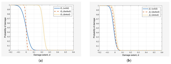
Figure 7.
Probabilistic curves for the D1 case. (a) Probabilistic curves for . (b) Probabilistic curves for .
Similarly, for Damage Case 2, it can be observed from Figure 8a,b that with 10% damage and with 20% damage exhibit probabilities of damage of 49.74% and 50.74%, respectively. In contrast, , , and , under both 10% and 20% damage scenarios, show very low probabilities of damage.
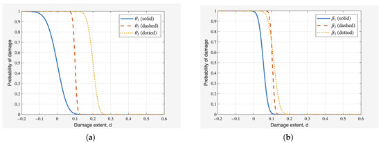
Figure 8.
Probabilistic curves for the D2 case. (a) Probabilistic curves for . (b) Probabilistic curves for .
In conclusion, while this approach demonstrated robust performance in detecting and quantifying stiffness degradation, its effectiveness in identifying mass changes was limited.
4.2. Considering Non-Uniform Temperature
To simulate more realistic conditions, the proposed updating method was applied under a non-uniform temperature distribution, as illustrated in Figure 9. In this scenario, the structure is subjected to varying temperatures, with the left side experiencing higher temperatures due to direct solar radiation. At each story level, the two columns on the left are exposed to elevated temperatures—50 °C at the top, 45 °C in the middle, and 30 °C at the bottom—while the corresponding columns on the right maintain lower, uniform temperatures of 30 °C at the top, 28 °C in the middle, and 20 °C at the bottom. This thermal gradient from top to bottom captures a more realistic environmental condition for structural assessment.
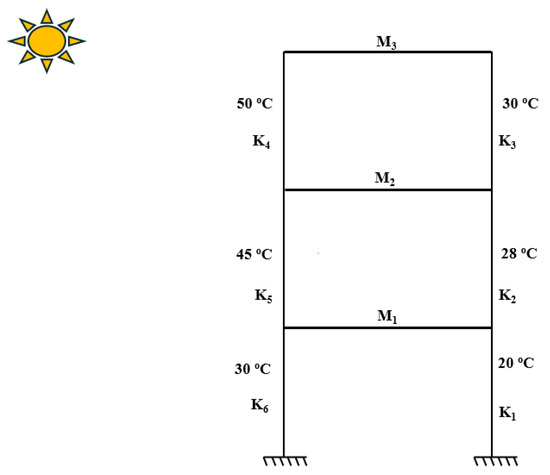
Figure 9.
Three-story shear building at non-uniform temperature.
To compute the change in the stiffness matrix due to temperature, the stiffness variation is calculated for each pair of columns based on their respective temperature-induced change in elastic modulus and geometric matrix. These individual contributions are then assembled to form the global stiffness change matrix for the entire structure. However, in the current implementation, the same stiffness parameter, , is used for all columns of each story. This simplification may limit the accuracy in cases where column-specific thermal properties vary significantly. Future work is needed to incorporate column-specific values to more accurately represent material variability and thermal exposure differences across the structure.
Table 9 shows the mode frequency comparison between the measured and updated values, which shows that the error between updated and target/measured at 20 °C is less than 0.05%.
Table 9.
Modal frequency (Hz) comparison of measured and updated for non-uniform case.
Table 10 shows the updated stiffness and mass parameters for the healthy case. The identified stiffness parameters (, , and ) closely match the target values of 1.0000, with low standard deviations and coefficients of variation, indicating high reliability. Although the identified mass parameters (, , and ) are numerically close to the targets, they lie outside the confidence interval based on their respective standard deviations.
Table 10.
Updated stiffness and mass parameters (healthy case).
A likely reason is that temperature deviations primarily affect stiffness rather than mass. As a result, the stiffness parameters were well-identified, accurately reflecting the temperature variations in both states. In contrast, the mass parameters were poorly identified, with the updated values poorly distributed across individual degrees of freedom. This outcome can be attributed to one or both of two reasons. The optimization process may have become trapped in a local optimum by primarily minimizing the error. Additionally, the mass parameters themselves may have been relatively insensitive to modal parameters (frequencies and mode shapes), making them difficult for the proposed algorithm to properly identify accurately. For example, Kim et al. [45] reported that the uneven mass distribution in a large structure may change only limited natural frequencies but remain unchanged in mode shapes using the damage detection algorithm.
One approach to mitigating uncertainties is to use the mass-change FEMU method, as discussed in Zeng and Kim (2022) [23], in combination with a temperature-induced model updating scheme. Combining this approach with a temperature-induced model updating scheme creates a hybrid method. Further research is required to mitigate the model bias. Once the stiffness parameters are identified, the corresponding mass parameters can then be determined to minimize errors.
Figure 10 illustrates the MAC comparison between the target and updated mode shapes; the diagonal elements exhibit the values of 1, indicating that the updated model closely matches the measured mode shapes for the corresponding modes.
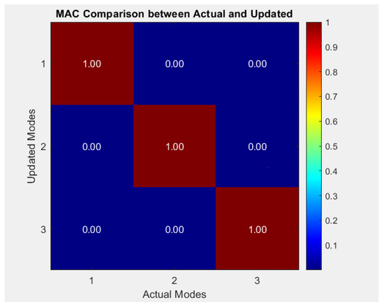
Figure 10.
Comparison of MAC between target and updated modes.
Damage Case D1 was simulated on the right two columns of the third story. As shown in Table 11, the identified stiffness parameters and closely match the target values, indicating no significant damage. In contrast, while shows a clear deviation from its target of 0.7850, it does not match the target case because the updated parameter is distributed to all four columns of the third story rather than two. For the mass parameters, appears to be close to the target value of 1.0000; however, all three identified mass parameters lie outside the confidence interval based on their respective standard deviations. Specifically, and deviate from their target values of 0.8925, indicating that, despite the apparent numerical closeness in some cases, the mass parameter identification is inconsistent under this damage condition. This indicates the challenge of identifying localized stiffness degradation under thermal gradients. Additionally, mass parameters deviated from their targets despite low uncertainty. Also, probabilistic results showed that , , and exhibited very low probabilities of damage, despite the presence of assumed damage levels.
Table 11.
Updated stiffness and mass parameters for Damage No.1.
Table 12 presents a comparison of the measured (non-uniform temperature) and updated natural frequencies for the damage case. The first and second mode frequencies show excellent agreement, with minimal errors of and , respectively. The third mode exhibits a larger error of , which can be attributed to inaccuracies in the identification of the stiffness parameter.
Table 12.
Target and updated frequencies (Hz) for Damage No.1.
The probability of damage was calculated for both mass and stiffness parameters. As shown in Figure 11a,b, the parameters , , and exhibit very low probabilities of damage, even under assumed damage levels of 21.8% for the stiffness parameter and 21.5% for the mass parameters.
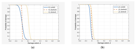
Figure 11.
Probabilistic curves for the D1 case. (a) Probabilistic curves for . (b) Probabilistic curves for .
These errors likely come from an overly simple model. Using a model with a higher degree of freedom would capture column-level changes and improve localization. Alternatively, this method can be combined with a partial-model method [35] that estimates stiffness in small substructures—so you do not need a full global model and can pin down local damage more reliably.
In summary, under the healthy condition, all stiffness parameters (–) had percentage errors below 0.05% and fell within their target ± standard deviation ranges, indicating excellent accuracy. In contrast, mass parameters (–) showed small percentage errors (up to 0.6%), but due to their extremely low standard deviations (∼10−8), the identified values fell outside the uncertainty bounds.
In Damage Case 1 (uniform temperature), stiffness estimates remained accurate with errors under 0.41%, all within their standard deviations reported in Table 6. However, mass parameters showed larger discrepancies: – had errors ranging from 3.70% to 13.83%, all exceeding their respective uncertainty bounds, indicating systematic bias despite low C.O.V. values. The results indicate a significant probability of damage (50.4%) in at a possible damage level of 21.8%, while the mass parameters and exhibit very low probabilities of damage at a comparable damage level of 21.5%.
In Damage Case 2, the stiffness parameters again closely matched the target values, as reported in Table 7. Mass parameters and were within acceptable bounds, but had a 6.22% error, exceeding its uncertainty range. For probabilistic damage detection, with 10% damage and with 20% damage exhibit notable probabilities of damage at 49.74% and 50.74%, respectively. In contrast, the mass parameters , , and show very low probabilities of damage under both 10% and 20% damage scenarios.
Under non-uniform temperature, performance declined. While and remained accurate, deviated significantly (13.1% error, outside ±0.0128). All mass parameters exceeded their uncertainty bounds, with errors up to 12%, indicating reduced reliability in localized damage detection under thermal gradients. For probabilistic damage detection, the results show that , , and exhibit very low probabilities of damage, despite assumed damage levels of 21.8% for stiffness and 21.5% for mass parameters.
5. Conclusions
This paper introduces a novel BMUA framework that incorporates temperature-induced variations, which affect the structural stiffness matrix. Simulated data under two distinct thermal conditions—consisting of natural frequencies and mode shapes—are used to evaluate the framework. These simulated responses enable the decoupling of the mass and stiffness updating processes, thereby removing the need for prior assumptions about the mass matrix. The main conclusions and contributions of this work are summarized below:
- The proposed updating approach effectively updates both mass and stiffness while addressing the coupling effect by using temperature variation that changes the stiffness of the structure. Unlike previous research methods that require physical modifications, such as adding mass or stiffness to create a modified system, which is often impractical in real-world scenarios, this approach offers a practical way that relies solely on naturally occurring temperature changes.
- The proposed updating approach effectively eliminates temperature-induced changes in natural frequencies and mode shapes, helping to ensure that structural damage is not obscured by temperature.
- Under uniform temperature, the proposed BMUA accurately identified stiffness; however, the mass parameters fall outside of the uncertainty range. Under non-uniform temperature, localized damage accuracy declined, falling outside of the uncertainty range, likely due to an overly simple model.
Although the proposed BMUA shows promise for SHM, several steps remain for future work. First, it should be validated against both laboratory and field measurements. Second, it should be applied to additional structures (e.g., trusses and bridges). Third, the model should include a more realistic thermal heat transfer process and more updating parameters to account for localized damages. Finally, the framework should also be integrated with mass-perturbation FEMU approaches to eliminate errors for the identification of mass parameters.
Author Contributions
Conceptualization, Y.H.K.; methodology, U.A.; software, U.A.; validation, Y.H.K.; writing—original draft preparation, U.A.; writing—review and editing, Y.H.K.; supervision, Y.H.K. All authors have read and agreed to the published version of the manuscript.
Funding
This research received no external funding.
Data Availability Statement
The codes and associated raw data supporting the conclusions of this article will be made available by the authors on request.
Conflicts of Interest
The authors declare no conflicts of interest.
Nomenclature
The following nomenclature are used in this manuscript:
| Symbol | Description |
| Eigenvalue (square of natural frequency) | |
| Natural frequency | |
| Eigenvalue of modified structure | |
| Natural frequency of modified structure | |
| Measured eigenvalue | |
| Mode shape (eigenvector) | |
| Mode shape (eigenvector) of modified structure | |
| Measured mode shape | |
| Mass matrix | |
| Stiffness matrix | |
| Damping matrix | |
| Change in stiffness matrix due to temperature | |
| Change in elastic stiffness matrix due to temperature | |
| Vector of uncertainty parameters | |
| C | Structural model class |
| D | Measured data |
| Prior probability density function | |
| Likelihood function of observed data D | |
| Posterior probability density function of parameters | |
| Normalizing constant (also denoted as ) | |
| Eigen-equation error when updating mass | |
| Eigen-equation error when updating stiffness | |
| Number of measured modes | |
| Total number of modes | |
| Stiffness parameter vector | |
| Mass parameter vector | |
| Covariance matrix of measurement error | |
| Covariance matrix of prior mass parameters | |
| Covariance matrix of prior stiffness parameters | |
| exp | Exponential function |
| The lth elemental stiffness matrix | |
| The lth elemental mass matrix | |
| Constant stiffness matrix (set as zero) | |
| Constant mass matrix (set as zero) | |
| d | Fractional damage level |
| Probability of damage at damage extent d | |
| The cumulative distribution function | |
| The standard deviation | |
| Variance of eigen-equation error | |
| Objective function for mass updating | |
| Objective function for stiffness updating | |
| Constant in prior probability density functions | |
| Mode shape matching matrix (selection) | |
| , | Residual matrices for mass and stiffness |
| , | Coefficients of variation for simulated data |
| Measurement noise (Gaussian error) | |
| Covariance matrix of updated parameters | |
| Nominal parameters of | |
| Updated parameters of | |
| E | Young’s modulus |
| Young’s modulus at 20 °C | |
| Coefficient of elastic modulus | |
| Elastic stiffness matrix at reference temperature | |
| Elastic stiffness matrix at different temperature | |
| Geometric stiffness matrix | |
| T | Temperature of element in degrees Celsius |
| Reference temperature | |
| Difference between T and | |
| I | Moment of inertia |
| A | Cross-sectional area |
| L | Element length |
| Coefficient of linear thermal expansion | |
| Axial spring stiffness | |
| Slope factor of spring associated with temperature increase | |
| Axial force due to thermal effect |
Appendix A. Calculation of Stiffness of Spring
Critical Force
The critical load to buckle the column is calculated based on Euler’s critical load formula. The effective length factor for this column is taken as 1 based on the assumption that it is simply supported.
Appendix B. Investigation of Mass Updating at Damaged Case
In Damage Case D1, the updated natural frequencies calculated using Equations (A42) and (A49) are compared with those calculated from the FEM using the updated parameters obtained through the model updating process. The table below summarizes the comparison.
| Mode | Updated Frequency (Hz) | FEM (Hz) | Percentage Difference (%) |
| 1 | 8.5535 | 8.5466 | 0.0807 |
| 2 | 22.5565 | 22.5192 | 0.1656 |
| 3 | 33.6341 | 33.4807 | 0.4582 |
As shown above, the natural frequencies calculated from the updated FEM closely match those obtained from the updated damage case. However, although the updated stiffness parameters closely matched the actual values and resulted in accurate reproduction of the natural frequencies, the updated mass parameters did not align well with the actual system. This highlights a remaining limitation in effectively capturing the coupling effects between mass and stiffness for this particular structure. As a result, there is still a gap in accurately identifying mass-related changes, which requires further investigation and methodological improvement in future studies.
Appendix C. Mathematical Derivation
Appendix C.1. Theoretical Background of BMUA
The proposed approach employs Bayesian probability theory to update structural parameters by integrating prior knowledge with measured data. The framework is based on Bayes’ theorem, which combines the prior distribution, likelihood function, and measured data to form the posterior probability density function (PDF). The posterior PDF represents the updated belief about the structural parameters given the observed data and is expressed as [46]
whereby
- D represents the vector of the measurements;
- represents the prior distribution;
- represents the likelihood function of the parameters;
- represents the evidence;
- represents the posterior distribution.
For this study, measured data are taken as the measured eigenvalue and mode shapes for model updating. is the structural physical parameters, including mass and stiffness parameters in this study. The posterior PDF for the unknown parameters is given by Bayes’ theorem:
where are updated eigenvalues, are updated mode shapes, and are parameters to be updated. are measured eigenvalues, are measured mode shapes, and the constant term is denoted by . A class of dynamical models C is considered with DOFs. The stiffness matrix is parameterized by as follows:
Similarly, the mass matrix is parameterized by as follows:
The lth stiffness parameter forms the lth elemental stiffness matrix, ; similarly, the mth mass parameter forms the mth elemental mass matrix, .
K0 are constant matrices and are set to zero for the sake of convenience. The scaling parameters and allow the nominal matrices to be updated based on dynamic test data from the system.
Appendix C.2. Probabilistic Damage Detection
The application of the BMUA allows damage detection and quantification. To better quantify the damage, the most probable values and standard deviations of the mass and stiffness parameters are used to calculate the probability that a specific parameter or has been reduced by a fraction relative to the undamaged state of the structure. The probability can be computed using updated parameters and corresponding standard deviations based on asymptotic Gaussian approximation [47,48].
where represents the cumulative distribution function of the standard Gaussian random variable, and denote the most probable values of the th mass and stiffness parameters for healthy and damaged structures, and and are corresponding standard deviations.
Appendix C.3. Derivation for Decoupling the Mass and Stiffness with Change of Stiffness
Similar to Equation (A7),
Let us assume and ; Equation (A10) is rewritten as
Therefore, is solved as another expression, :
Finally, eigen-equation error, , is reformulated when updating mass:
Similar derivation procedures for stiffness updating are employed, and is pre-multiplied as in Equation (A6):
The transposed matrix of Equation (A7) is first calculated, then the resulting equation is post-multiplied by :
Subtracting Equation (A16) from Equation (A17) gives
Defining and , Equation (A18) is simplified. Also, W’ expression is given by
Then, the eigen-equation error, , is reformulated when updating stiffness:
Appendix C.4. Formulation of the New Prior PDF with Δk
Assume modes are measured. The prior PDF in the proposed BMUA is chosen as when updating parameters, :
where and are eigenvalues and eigenvectors to be updated, respectively. is formulated using Gaussian PDF with the new eigen-equation error in Equation (A13):
where denotes a constant, the sign of denotes mathematical Euclidean norm, and denotes a defined variance of eigen-equation error. Equation (A27) is simplified as
where
where . denotes the covariance matrix in prior PDF; denotes an identity matrix. arises from the modeling error between theoretical and target FE models. Another term of in Equation (A21) is approximated by a Gaussian distribution, which has a mean value of (nominal value) and covariance matrix, , is selected as a large variance to let be a non-informative prior [36]. Hence, maybe expressed as
Appendix C.5. Formulation of Likelihood Function
Assuming a measurement error, ,
where the Gaussian distribution is assigned to . denotes the measured eigenvalues; denotes measured mode shapes. consists of ‘1s’ or ‘0s’ to match measured partial mode shapes with the theoretical counterparts. Therefore, the likelihood function is expressed as
where is the measured covariance matrix that can be obtained by Bayesian modal analysis, reflecting the effect of measurement noise on identified frequencies and mode shapes.
Appendix C.6. Formulation of Posterior PDF with Δk
Based on the formulation of the prior PDF in Equation (A26) and the likelihood function in Equation (A33), the posterior PDF for mass updating can be written as
The asymptotic approximation method is used to obtain MPVs of structural parameters in Equation (A29). The most probable values (MPVs) can be found by minimizing the objective functions, and analytical formulations of model parameters and uncertainty can be conveniently derived. The objective function with additional stiffness when updating mass parameters is expressed as
In terms of updating stiffness, , the same derivation is employed; the prior PDF has the expression
where are updated eigenvalues; are updated eigenvectors.
where . The likelihood function is given by
The objective function with additional stiffness when updating stiffness parameters is expressed as
Optimization Framework with Δk
MPVs of the updated parameters are determined using the asymptotic approximation technique applied to the objective functions given in Equations (A30) and (A34). The asterisk symbol ‘*’ indicates an updated value. The optimal values of are obtained by minimizing with respect to .
where is left bottom sub-matrix of ; is right bottom sub-matrix of . is defined as
where the sign of ‘diag’ indicates diagonal matrix.
Similarly, by optimizing Equation (A30) with respect to , the optimal is obtained as
where is the right top sub-matrix of ; is the left top sub-matrix of . is defined as
Similarly, by optimizing Equation (A30) with respect to , the optimal is obtained as
where and are expressed as
When updating stiffness, the optimal is obtained by optimizing Equation (A34) with respect to as
where is expressed as
where .
The optimal is expressed as
where is expressed as
The optimal stiffness parameter is obtained as
where and is expressed as
Initially and are defined as nominal values, respectively: , , and measured , which, in this study, are simulated by adding small Gaussian noise to the true natural frequencies and mode shapes obtained from the finite element model. A coefficient of variation (C.O.V) of 0.1% is used to mimic realistic measurement noise. The mathematical expression to generate simulated natural frequency and mode shape is given by Yuen [36]
Here, is the simulated (measured) squared natural frequency, is the reference (true) squared natural frequency, is the coefficient of variation (C.O.V.) for frequency (e.g., ), and is the standard normal random variable.
Here, is the simulated (measured) -th component of the mode shape, is the reference (true) -th component of the mode shape, is the coefficient of variation (C.O.V.) for mode shapes (e.g., ), is the total number of degrees of freedom, and is the standard normal random variable (independent for each ).
Appendix C.7. Uncertainty Quantification with Δk
When sufficient measurement data are available, the posterior probability density function (PDF) can be effectively approximated using a Gaussian distribution. In this context, the mean and covariance matrix of the Gaussian are represented by the MPVs of the updated parameters and the inverse of the Hessian matrix of the objective function, respectively. This covariance matrix serves to express the uncertainty associated with the model parameters [36]. The covariance matrix of in the case of mass updating is given by
where , and is given by
Similarly, the covariance matrix of when updating stiffness is described as
where , and are defined as
Once the covariance matrix is obtained, the standard deviations of the updated parameters can be determined by taking the square root of the diagonal elements of .
References
- Friswell, M.I.; Mottershead, J.E. Finite element modelling. In Finite Element Model Updating in Structural Dynamics; Springer: Dordrecht, The Netherlands, 1995; pp. 7–35. [Google Scholar]
- Hemez, F.M.; Doebling, S.W. Review and assessment of model updating for non-linear, transient dynamics. Mech. Syst. Signal Process. 2001, 15, 45–74. [Google Scholar] [CrossRef]
- Kong, X.; Cai, C.S.; Hu, J. The state-of-the-art on framework of vibration-based structural damage identification for decision making. Appl. Sci. 2017, 7, 497. [Google Scholar] [CrossRef]
- Chen, H.P. Structural Health Monitoring of Large Civil Engineering Structures; Wiley: Hoboken, NJ, USA, 2018. [Google Scholar]
- Alkayem, N.F.; Cao, M.; Zhang, Y.; Bayat, M.; Su, Z. Structural damage detection using finite element model updating with evolutionary algorithms: A survey. Neural Comput. Appl. 2018, 30, 389–411. [Google Scholar] [CrossRef]
- Sun, H.; Büyüköztürk, O. The MIT Green Building benchmark problem for structural health monitoring of tall buildings. Struct. Control Health Monit. 2018, 25, e2115. [Google Scholar] [CrossRef]
- Luo, L.; Xia, Y.; Wang, A.; Lei, X.; Jian, X.; Sun, L. Finite element model updating method for continuous girder bridges using monitoring responses and traffic videos. Struct. Control Health Monit. 2022, 29, e3062. [Google Scholar] [CrossRef]
- Jensen, H.; Papadimitriou, C. Sub-Structure Coupling for Dynamic Analysis; Springer: Cham, Switzerland, 2019. [Google Scholar]
- Jensen, H.; Vergara, C.; Papadimitriou, C.; Millas, E. The use of updated robust reliability measures in stochastic dynamical systems. Comput. Methods Appl. Mech. Eng. 2013, 267, 293–317. [Google Scholar] [CrossRef]
- Simoen, E.; De Roeck, G.; Lombaert, G. Dealing with uncertainty in model updating for damage assessment: A review. Mech. Syst. Signal Process. 2015, 56, 123–149. [Google Scholar] [CrossRef]
- Mottershead, J.E.; Link, M.; Friswell, M.I. The sensitivity method in finite element model updating: A tutorial. Mech. Syst. Signal Process. 2011, 25, 2275–2296. [Google Scholar] [CrossRef]
- Soize, C.; Capiez-Lernout, E.; Ohayon, R. Robust updating of uncertain computational models using experimental modal analysis. AIAA J. 2008, 46, 2955–2965. [Google Scholar] [CrossRef]
- Sipple, J.D.; Sanayei, M. Finite element model updating of the UCF grid benchmark using measured frequency response functions. Mech. Syst. Signal Process. 2014, 46, 179–190. [Google Scholar] [CrossRef]
- Chen, H.P.; Maung, T.S. Regularised finite element model updating using measured incomplete modal data. J. Sound Vib. 2014, 333, 5566–5582. [Google Scholar] [CrossRef]
- Hekič, D.; Ribeiro, D.; Anžlin, A.; Žnidarič, A.; Češarek, P. Improved Finite Element Model Updating of a Highway Viaduct Using Acceleration and Strain Data. Sensors 2024, 24, 2788. [Google Scholar] [CrossRef]
- Katafygiotis, L.S.; Beck, J.L. Updating models and their uncertainties. II: Model identifiability. J. Eng. Mech. 1998, 124, 463–467. [Google Scholar] [CrossRef]
- Hurtado, O.D.; Ortiz, A.R.; Gomez, D.; Astroza, R. Bayesian model-updating implementation in a five-story building. Buildings 2023, 13, 1568. [Google Scholar] [CrossRef]
- Lam, H.F.; Hu, J.; Adeagbo, M.O. Bayesian model updating of a 20-story office building utilizing operational modal analysis results. Adv. Struct. Eng. 2019, 22, 3385–3394. [Google Scholar] [CrossRef]
- Asadollahi, P.; Huang, Y.; Li, J. Bayesian finite element model updating and assessment of cable-stayed bridges using wireless sensor data. Sensors 2018, 18, 3057. [Google Scholar] [CrossRef] [PubMed]
- Luo, L.; Song, M.; Zhong, H.; He, T.; Sun, L. Hierarchical Bayesian model updating of a long-span arch bridge considering temperature and traffic loads. Mech. Syst. Signal Process. 2024, 210, 111152. [Google Scholar] [CrossRef]
- Cheung, S.H.; Bansal, S. A new Gibbs sampling based algorithm for Bayesian model updating with incomplete complex modal data. Mech. Syst. Signal Process. 2017, 92, 156–172. [Google Scholar] [CrossRef]
- Do, N.T.; Gül, M. Structural damage detection under multiple stiffness and mass changes using time series models and adaptive zero-phase component analysis. Struct. Control Health Monit. 2020, 27, e2577. [Google Scholar] [CrossRef]
- Zeng, J.; Kim, Y.H. Identification of Structural Stiffness and Mass using Bayesian Model Updating Approach with Known Added Mass: Numerical Investigation. Int. J. Struct. Stab. Dyn. 2020, 20, 2050123. [Google Scholar] [CrossRef]
- Xia, Y.; Chen, B.; Weng, S.; Ni, Y.Q.; Xu, Y.L. Temperature effect on vibration properties of civil structures: A literature review and case studies. J. Civ. Struct. Health Monit. 2012, 2, 29–46. [Google Scholar] [CrossRef]
- Farrar, C.R.; Doebling, S.W.; Cornwell, P.J.; Straser, E.G. Variability of Modal Parameters Measured on the Alamosa Canyon Bridge; Technical Report; Los Alamos National Lab. (LANL): Los Alamos, NM, USA, 1996. [Google Scholar]
- Askegaard, V.; Mossing, P. Long Term Observation of Rc-Bridge Using Changes in Natural Frequency. Nordic Concrete Research. Publication no 7; Nordic Concrete Federation: Oslo, Norway, 1988. [Google Scholar]
- Desjardins, S.L.; Londono, N.A.; Lau, D.T.; Khoo, H. Real-time data processing, analysis and visualization for structural monitoring of the confederation bridge. Adv. Struct. Eng. 2006, 9, 141–157. [Google Scholar] [CrossRef]
- Mosavi, A.A.; Seracino, R.; Rizkalla, S. Effect of temperature on daily modal variability of a steel-concrete composite bridge. J. Bridge Eng. 2012, 17, 979–983. [Google Scholar] [CrossRef]
- Zeng, J.; Kim, Y.H. Stiffness Modification-Based Bayesian Finite Element Model Updating to Solve Coupling Effect of Structural Parameters: Formulations. Appl. Sci. 2021, 11, 10615. [Google Scholar] [CrossRef]
- Zeng, J.; Kim, Y.H. Probabilistic damage detection and identification of coupled structural parameters using Bayesian model updating with added mass. J. Sound Vib. 2022, 539, 117275. [Google Scholar] [CrossRef]
- Zhou, H.; Ni, Y.; Ko, J. Eliminating temperature effect in vibration-based structural damage detection. J. Eng. Mech. 2011, 137, 785–796. [Google Scholar] [CrossRef]
- Wang, Z.; Yi, T.H.; Yang, D.H.; Li, H.N.; Liu, H. Eliminating the bridge modal variability induced by thermal effects using localized modeling method. J. Bridge Eng. 2021, 26, 04021073. [Google Scholar] [CrossRef]
- Lee, Y.; Kim, H.; Min, S.; Yoon, H. Structural damage detection using deep learning and FE model updating techniques. Sci. Rep. 2023, 13, 18694. [Google Scholar] [CrossRef]
- Zhou, S.; Song, W. Updating finite element models considering environmental impacts. In Proceedings of the Sensors and Smart Structures Technologies for Civil, Mechanical, and Aerospace Systems 2016, Las Vegas, NV, USA, 20–24 March 2016; SPIE: Bellingham, WA, USA, 2016; Volume 9803, pp. 509–516. [Google Scholar]
- Xiao, F.; Mao, Y.; Tian, G.; Chen, G.S. Partial-model-based damage identification of long-span steel truss bridge based on stiffness separation method. Struct. Control Health Monit. 2024, 2024, 5530300. [Google Scholar] [CrossRef]
- Yuen, K.V. Bayesian Methods for Structural Dynamics and Civil Engineering; John Wiley & Sons: Hoboken, NJ, USA, 2010. [Google Scholar]
- Hızal, Ç.; Turan, G. A two-stage Bayesian algorithm for finite element model updating by using ambient response data from multiple measurement setups. J. Sound Vib. 2020, 469, 115139. [Google Scholar] [CrossRef]
- Sun, K.; Zhao, Y.; Hu, H. Identification of temperature-dependent thermal–structural properties via finite element model updating and selection. Mech. Syst. Signal Process. 2015, 52–53, 147–161. [Google Scholar] [CrossRef]
- Paz, M.; Kim, Y. Structural Dynamics: Theory and Computation; Springer International Publishing: Berlin/Heidelberg, Germany, 2018. [Google Scholar]
- Adhikari, U. Bayesian Model Updating of Structural Parameters Using Temperature Variation Data. Master’s Thesis, Electronic Theses and Dissertations, Paper 4546. University of Louisville, Louisville, KY, USA, 2025. [Google Scholar]
- Cui, D.; Hu, H. Thermal buckling and natural vibration of the beam with an axial stick–slip–stop boundary. J. Sound Vib. 2014, 333, 2271–2282. [Google Scholar] [CrossRef]
- Yuan, Z.; Yu, K.; Bai, Y. A multi-state model updating method for structures in high-temperature environments. Measurement 2018, 121, 317–326. [Google Scholar] [CrossRef]
- Zeng, J. Hybrid Structural Health Monitoring Using Data-Driven Modal Analysis and Model-Based Bayesian Inference. Ph.D. Thesis, Electronic Theses and Dissertations, Paper 3791. University of Louisville, Louisville, KY, USA, 2021. [Google Scholar] [CrossRef]
- Allemang, R.J. The modal assurance criterion–twenty years of use and abuse. Sound Vib. 2003, 37, 14–23. [Google Scholar]
- Kim, J.T.; Ryu, Y.S.; Cho, H.M.; Stubbs, N. Damage identification in beam-type structures: Frequency-based method vs mode-shape-based method. Eng. Struct. 2003, 25, 57–67. [Google Scholar] [CrossRef]
- Bayes, T. LII. An essay towards solving a problem in the doctrine of chances. By the late Rev. Mr. Bayes, FRS communicated by Mr. Price, in a letter to John Canton, AMFR S. Philos. Trans. R. Soc. Lond. 1763, 53, 370–418. [Google Scholar] [CrossRef]
- Mustafa, S.; Matsumoto, Y. Bayesian model updating and its limitations for detecting local damage of an existing truss bridge. J. Bridge Eng. 2017, 22, 04017019. [Google Scholar] [CrossRef]
- Das, A.; Debnath, N. A Bayesian model updating with incomplete complex modal data. Mech. Syst. Signal Process. 2020, 136, 106524. [Google Scholar] [CrossRef]


Disclaimer/Publisher’s Note: The statements, opinions and data contained in all publications are solely those of the individual author(s) and contributor(s) and not of MDPI and/or the editor(s). MDPI and/or the editor(s) disclaim responsibility for any injury to people or property resulting from any ideas, methods, instructions or products referred to in the content. |
© 2025 by the authors. Licensee MDPI, Basel, Switzerland. This article is an open access article distributed under the terms and conditions of the Creative Commons Attribution (CC BY) license (https://creativecommons.org/licenses/by/4.0/).