Abstract
In field exploration, disaster rescue, and complex terrain operations, the accuracy of ground type recognition directly affects the walking stability and task execution efficiency of legged robots. To address the problem of terrain recognition in complex ground environments, this paper proposes a high-precision classification method based on single-leg triaxial force signals. The method first employs a one-dimensional convolutional neural network (1D-CNN) module to extract local temporal features, then introduces a long short-term memory (LSTM) network to model long-term and short-term dependencies during ground contact, and incorporates a convolutional block attention module (CBAM) to adaptively enhance the feature responses of critical channels and time steps, thereby improving discriminative capability. In addition, an improved whale optimization algorithm (iBWOA) is adopted to automatically perform global search and optimization of key hyperparameters, including the number of convolution kernels, the number of LSTM units, and the dropout rate, to achieve the optimal training configuration. Experimental results demonstrate that the proposed method achieves excellent classification performance on five typical ground types—grass, cement, gravel, soil, and sand—under varying slope and force conditions, with an overall classification accuracy of 96.94%. Notably, it maintains high recognition accuracy even between ground types with similar contact mechanical properties, such as soil vs. grass and gravel vs. sand. This study provides a reliable perception foundation and technical support for terrain-adaptive control and motion strategy optimization of legged robots in real-world environments.
1. Introduction
Legged robots exhibit excellent mobility in complex terrain environments and have been widely deployed in field exploration, disaster rescue, and other mission scenarios. The locomotion stability of legged robots largely depends on terrain classification methods with high real-time performance and accuracy. Inadequate ground perception may prevent the control system of legged robots from promptly and accurately adjusting gait parameters, resulting in unstable motion, increased energy consumption, or even mission failure. Existing terrain recognition methods can be generally categorized into three types: vision-based approaches, proprioception-based approaches, and multimodal fusion strategies.
Vision-based methods mainly rely on cameras to capture terrain appearance and geometric information for classification. In 2019, Cheng et al. [1] applied a convolutional neural network to road surface images and achieved an overall accuracy of 94.89%. In 2020, Šabanovič et al. [2] employed video inputs and deep neural networks to classify six types of road surfaces and conditions, obtaining an average accuracy of 88.8%, with 96% for surface-type classification. In 2022, Laschowski et al. [3] utilized wearable cameras and deep CNNs for environment classification in robotic leg prostheses and exoskeletons, achieving 73.2% accuracy across 12 classes. In 2024, Chen et al. [4] proposed a CNN-based fusion of RGB and NIR images for terrain classification, achieving 95.9% and 99.7% accuracy, respectively. In the same year, Pešek [5] applied U-Net and DeepLabv3+ for aerial image road material segmentation, with an overall accuracy of ~92%. Jiang et al. [6] (2024) introduced a WOA-BP-based multi-sensor fusion approach for road surface condition detection, achieving 98.8% average accuracy.
Proprioception-based methods rely on onboard sensors such as force, vibration, and IMU to capture dynamic interaction signals. In 2019, Wu et al. [7] integrated capacitive tactile sensors and IMU signals with SVM, achieving 82.5% accuracy across eight terrains. Mei et al. [8] (2019) proposed a 1D-CNN-LSTM model using vibration data, achieving 80.18% accuracy. Bai et al. [9] (2019) combined IMU vibration signals with an MLP, achieving up to 98% recognition accuracy. In 2021, Vulpi et al. [10] applied CNN/RNNs solely on proprioceptive inputs, achieving robust terrain classification in off-road environments. Wang et al. [11] (2021) developed an adaptive online classifier using vibration features and random forests, reaching nearly 98% accuracy. Bednarek et al. [12] (2022) proposed a Transformer-based haptic model with 92.7% accuracy under low-latency inference. Ugenti et al. [13] (2022) demonstrated that optimized signal selection with deep CNNs achieved 96.4% accuracy while reducing computational cost. Lv et al. [14] (2023) classified wheel–terrain interactions based on vibration signals, achieving 92.36%. Sarcevic et al. [15] (2023) utilized IMU and magnetometer signals with a lightweight MLP, enabling real-time terrain classification with >93% accuracy. In 2025, Zhang et al. [16] fused IMU and encoder data for multi-label terrain attribute recognition, achieving 96% average accuracy.
Multimodal fusion approaches combine visual and proprioceptive signals to enhance accuracy and robustness. In 2008, Halatci et al. [17] demonstrated terrain classification for planetary rovers by fusing vision and tactile/vibration signals, significantly improving performance over unimodal methods. In 2021, Chen et al. [18] proposed a vision CNN fused with proprioceptive 1D-CNN, achieving >93% overall accuracy. Haddeler et al. [19] (2022) integrated RGB-D and probe force signals to construct traversability maps with real-world validation. In 2023, Wang et al. [20] proposed feature-level fusion of image texture and vibration data with an improved WKNN algorithm, achieving 97.14% accuracy at 0.3 m/s and 91.43% at 0.7 m/s on tracked robots. Prágr et al. [21] (2023) introduced online learning with vision–tactile fusion for predicting the traversability of visually rigid but passable obstacles. In 2024, Chen et al. [4] fused RGB/NIR vision with a reduced-order proprioceptive model, achieving ~99.3% and 99.7% accuracy across eight terrain classes.
In summary, although significant progress has been made in vision-based, proprioception-based, and multimodal fusion approaches for terrain classification, several limitations remain. Vision-based methods are highly susceptible to variations in illumination, occlusion, and adverse weather, leading to unstable recognition performance. Proprioception-based methods avoid such environmental disturbances but often rely heavily on specific sensor characteristics and may lack robustness under varying slopes and complex loading conditions. Multimodal fusion strategies combine the advantages of both modalities, yet they face challenges in data synchronization, feature alignment, and computational complexity. To address these limitations, this study proposes a terrain classification method based on single-foot 3D force sensor signals. A hybrid 1D-CNN-LSTM model enhanced with the Convolutional Block Attention Module (CBAM) is developed, and an improved Whale Optimization Algorithm (iBWOA) is introduced to perform automated global optimization of critical hyperparameters, thereby enhancing both classification accuracy and generalization capability under complex terrain conditions.
2. Experimental Platform Design
To investigate the force response characteristics of legged robots under different ground conditions and address the problem of ground type recognition, a single-leg experimental platform was designed and constructed in this study as a substitute for full hexapod experiments. Compared with full-system experiments, this platform preserves the repeatability of foot–ground interactions while effectively reducing structural complexity and avoiding disturbances caused by multi-leg coordination, thereby allowing the study to focus on the intrinsic mechanisms of foot–ground interaction. Furthermore, the platform supports independent adjustment of force magnitude, gait rhythm, and ground conditions, enabling the construction of systematic and repeatable datasets to provide high-quality support for the training and validation of ground type recognition models. Overall, the single-leg experimental platform offers significant advantages in experimental feasibility, data accuracy, and research focus. Its findings can also be extended to hexapod robots, providing a solid foundation for terrain adaptability control and locomotion strategy optimization in real-world environments. The mechanical structure of the platform is illustrated in Figure 1.
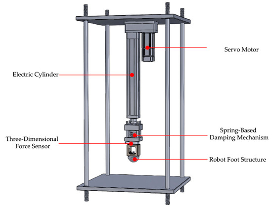
Figure 1.
The mechanical structure of the experimental platform.
The servo motor is mounted at the top of the platform and, in coordination with the electric cylinder, controls the longitudinal motion of the entire system. The electric cylinder converts the rotational motion of the servo motor into linear motion, driving the mechanical foot to perform vertical reciprocating movements. By adjusting the rotation speed and the number of revolutions of the servo motor, the velocity and displacement of the foot motion can be precisely controlled.
The spring-based damping mechanism is installed between the electric cylinder and the three-dimensional force sensor to provide a certain buffer stroke during high-intensity impacts, preventing damage to the sensor caused by rigid collisions. The three-dimensional force sensor is mounted between the spring mechanism and the robot foot, enabling real-time measurement of force variations along the X, Y, and Z axes of the foot. The terminal component of the system is the simulated robotic foot.
During data acquisition, the three-axis force sensor mounted on the robot’s foot measures, in real time, the variations in ground reaction forces along the X, Y, and Z directions. Each experiment simulated a complete step cycle comprising five distinct phases: pre-contact, contact, stabilization, lift-off, and post-contact. For each trial, the force sensor recorded 1024 continuous time-series data points across all three axes.
The experiments covered a wide range of locomotion and terrain conditions. Three different impact force levels (144 N, 180 N, 240 N) were applied to emulate pentapod, quadruped, and tripod gait loading conditions, respectively. The robotic foot interacted with five terrain types—soil, cement, gravel, grass, and sand—each tested under four slope angles (0°, 5°, 10°, 20°). For each combination of force level, terrain type, and slope angle, eight repeated trials were performed, resulting in a comprehensive dataset that reflects the variability in ground reaction forces due to both environmental and locomotion factors. The data acquisition experiment scenario is shown in Figure 2.
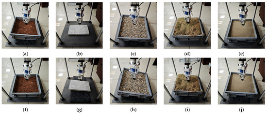
Figure 2.
Experimental scenarios under different terrain types and slope conditions. (a) Flat soil terrain, simulating natural loose soil in flat terrain; (b) Flat cement terrain, simulating high-stiffness, low-damping artificial hard ground; (c) Flat gravel terrain, simulating irregular rigid particle ground; (d) Flat grass terrain, simulating soft surface ground covered with vegetation; (e) Flat sand terrain, simulating loose, low-bearing-capacity non-cohesive particle ground; (f) Sloped soil terrain, simulating sloped terrain with loose soil; (g) Sloped cement terrain, simulating sloped terrain with hard ground; (h) Sloped gravel terrain, simulating sloped terrain with irregular particle ground; (i) Sloped grass terrain, simulating sloped terrain covered with vegetation; (j) Sloped sand terrain, simulating sloped terrain with loose particle ground.
3. 1D-CNN-LSTM-CBAM Model Building
The 1D-CNN–LSTM–CBAM ground recognition classification model developed in this study consists of five functional modules: an input layer, a convolutional feature extraction module, a CBAM attention mechanism module, a long short-term memory (LSTM) network module, and a classification output module. The structural diagram of the 1D-CNN–LSTM–CBAM ground recognition classification model is shown in Figure 3.
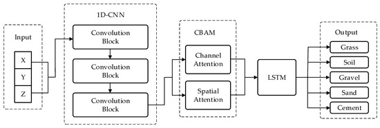
Figure 3.
The overall architecture diagram of the model.
The input layer receives time-series data collected by a three-axis force sensor. Subsequently, three one-dimensional convolutional blocks are employed to extract multi-scale local temporal features, which are then fed into the Convolutional Block Attention Module (CBAM) for feature reweighting and optimization. The attention-enhanced high-dimensional features are passed to a Long Short-Term Memory (LSTM) network to capture both long- and short-term dependencies in the ground contact process. Finally, the fully connected layer and Softmax classifier produce the output, enabling accurate classification of five representative terrain types: grass, cement, gravel, soil, and sand.
3.1. One-Dimensional Convolutional Neural Network Module
To effectively extract local temporal features embedded in the tri-axial force sensor signals collected during the single-leg stepping process of the legged robot, a one-dimensional convolutional neural network (1D-CNN) module is designed. This module performs feature extraction and preliminary representation learning on the input three-channel time-series data. Within the overall model architecture, it serves as the front-end perception component, providing essential feature support for the subsequent attention mechanism and long short-term memory (LSTM) layers. The structure of this module is illustrated in Figure 4.
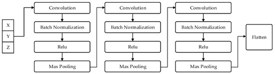
Figure 4.
The 1D CNN structure diagram.
The 1D-CNN module consists of three convolutional units, each comprising a convolutional layer, a batch normalization layer, an activation layer, and a max-pooling layer. The three convolutional layers extract local features under different receptive fields, progressively capturing multi-scale temporal dependencies. The numbers of convolution kernels are set to 64, 128, and 256, corresponding to the hierarchical extraction of low-, mid-, and high-level features.
Batch normalization is applied after each convolutional layer to alleviate the vanishing gradient problem, stabilize the training process, accelerate convergence, and enhance generalization. The activation layers employ the ReLU function to introduce nonlinearity, enabling the network to learn more complex temporal patterns. Subsequently, max-pooling operations reduce the dimensionality of feature maps, decrease the parameter count, and retain the most discriminative features to improve computational efficiency.
Finally, the feature maps are flattened into one-dimensional vectors via a flatten layer, providing a unified input format for subsequent network modules and enabling cross-channel feature integration.
The convolution operation in the 1D-CNN module can be formally expressed as follows:
where represents the input sequence value at channel C and position , denotes the weight parameter at the j-th position of the k-th convolution kernel for channel c, is the bias term of the k-th convolution kernel, is the kernel size, represents the nonlinear activation function (ReLU in this work), and represents the convolution output of the k-th kernel at position i.
By stacking multiple convolutional layers with nonlinear activation functions, this module efficiently learns deep local features from raw sensor data that are highly relevant to ground-type classification. It demonstrates strong capability in capturing characteristic variations, including the instantaneous impact at ground contact, the sustained pressure during the stabilization phase, and the decreasing force trend during lift-off. These extracted features provide a solid foundation for subsequent temporal modeling via LSTM and attention enhancement through the CBAM.
3.2. Long Short-Term Memory (LSTM) Module
In hexapod robot ground recognition, the data collected by the three-dimensional force sensor exhibit pronounced temporal characteristics. To fully exploit the temporal dependencies and dynamic variation patterns within the sequential data, a long short-term memory (LSTM) network is incorporated on top of the local features extracted by the 1D-CNN module, enabling the modeling of both long-term and short-term dependencies along the temporal dimension.
As a special type of recurrent neural network (RNN), the long short-term memory (LSTM) network addresses the vanishing and exploding gradient problems commonly encountered in conventional RNNs when learning long sequences by introducing a gating mechanism. Its internal architecture comprises three primary gates—the forget gate, input gate, and output gate—which dynamically regulate the transmission and update of information within the cell state. The interactions among these gates within an LSTM unit are illustrated in Figure 5.
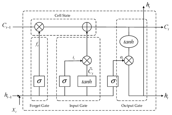
Figure 5.
Interaction Process of Gate Mechanisms in the LSTM Cell.
The forget gate takes the previous hidden state and the current input as inputs, and computes the forget vector via the Sigmoid activation function. This vector determines the proportion of the previous cell state to be retained. The formula is as follows:
where denotes the Sigmoid activation function, and represent the weight matrix of the forget gate, represent the bias term of the forget gate.
The input gate determines whether new information is written into the cell state at the current time step. Its control mechanism consists of two parallel branches: one updates the candidate cell state , while the other regulates the write intensity via a Sigmoid activation. The formula is as follows:
where denotes the input gate output at the current time step, controlling the extent to which the current input affects the cell state; and are the weight matrices for the input gate and the candidate state, respectively; and are the corresponding bias terms; denotes the hyperbolic tangent activation function, which compresses the values to the range [−1, 1] to represent candidate memory information.
The cell state is updated through the combined effect of the forget gate and the input gate. The formula is as follows:
The output gate determines the final hidden state output , which is jointly controlled by and . The formula is as follows:
where denotes the output gate activation at the current time step, and are the weight matrix and bias term of the output gate, respectively, and is the hyperbolic tangent activation function.
In the proposed classification model, the LSTM module adopts a single-layer architecture with 64 hidden units and incorporates dropout regularization to mitigate the risk of overfitting. By performing step-by-step modeling of the local feature sequences extracted by the 1D-CNN, the LSTM significantly enhances the model’s capability to capture temporal dependencies and dynamic evolution patterns associated with different terrain types. In particular, under varying slope and loading conditions, the LSTM module demonstrates strong generalization ability in recognizing complex terrain response patterns.
3.3. Convolutional Attention Module
To further enhance the model’s ability to perceive critical features, the Convolutional Block Attention Module (CBAM) was integrated into the CNN-LSTM backbone. CBAM consists of two sequential submodules, channel attention and spatial attention, which reweight feature maps along the channel and spatial dimensions, respectively. This process strengthens the network’s response to informative regions while suppressing irrelevant or redundant information, thereby improving its discriminative power in terrain classification. Specifically, the channel attention mechanism adaptively learns the weight distribution of tri-axial force features, enabling the model to focus on the most significant dimensions that reflect terrain hardness and dynamic responses. Meanwhile, the spatial attention mechanism emphasizes key temporal points, such as foot touchdown and stabilization phases, highlighting the dynamic differences across terrains during locomotion. The working principle of CBAM is illustrated in Figure 6.
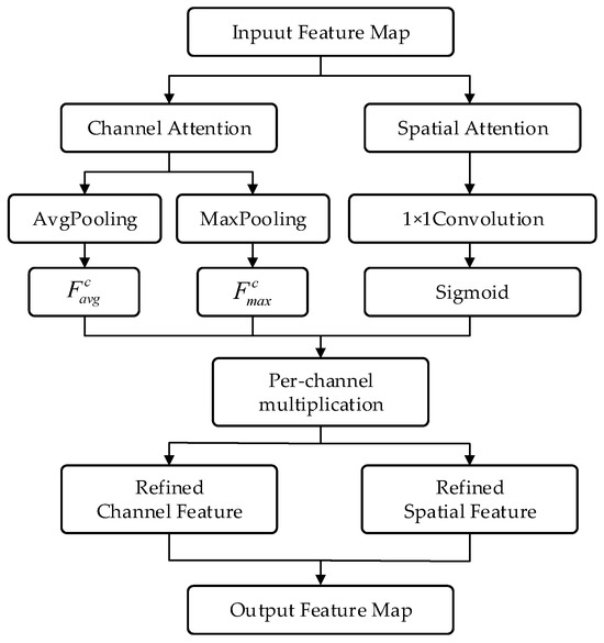
Figure 6.
The working principle diagram of the convolutional attention module.
The channel attention module aims to identify and emphasize the most discriminative channel features. In CBAM, the input feature map is first subjected to global average pooling and global max pooling along the spatial dimensions to generate two channel descriptor vectors, and . The formula is as follows:
Then, the two descriptor vectors are fed into a shared multi-layer perceptron (MLP), summed, and passed through a sigmoid activation function to obtain the channel attention weight. The formula is as follows:
where denotes the sigmoid activation function, and the MLP typically consists of one hidden layer followed by a ReLU activation function.
Finally, the input feature map is multiplied with the channel attention weights in a channel-wise element-wise manner to obtain the refined feature map . The formula is as follows:
where indicates channel-wise element-wise multiplication.
The spatial attention module focuses on “which locations in the feature map are more important.” Its input is the channel-refined feature map obtained from the previous step. First, global max pooling and global average pooling are performed along the channel dimension to produce two spatial feature maps, and . The formula is as follows:
The two spatial feature maps are concatenated along the channel dimension, passed through a convolutional layer, and then activated by a sigmoid function to generate the spatial attention map . The formula is as follows:
where denotes the sigmoid activation function, represents the convolution operation with a kernel size of , and indicates channel-wise concatenation.
The final output feature map is obtained by performing element-wise multiplication with broadcasting between the spatial attention map and the input feature map . The formula is as follows:
where represents element-wise multiplication with broadcasting.
The CBAM is embedded between the convolutional module and the LSTM module, serving as a bridge to reweight and optimize the extracted temporal features. In this study, particular emphasis is placed on enhancing the attention weights of the Z-axis features in the three-dimensional force sensor data, thereby enabling the model to more effectively focus on the most discriminative ground response signals during the robot’s stepping process.
3.4. Improved Beluga Whale Optimization Algorithm (IBWOA) Module
In deep neural networks, the proper configuration of hyperparameters—such as the number of convolutional filters, the number of LSTM units, and the dropout rate—has a significant impact on model performance. To improve the classification accuracy and generalization capability of the terrain classification model, this study introduces an Improved Beluga Whale Optimization Algorithm (iBWOA) for automated search and global optimization of key hyperparameters.
Traditional approaches, such as manual tuning and grid search, suffer from low efficiency and a high risk of being trapped in local optima, particularly in high-dimensional parameter spaces, making it difficult to obtain the global optimum. To address these limitations, we propose an enhanced version of the classical Beluga Whale Optimization Algorithm (BWOA), integrating global exploration with locally adaptive updating mechanisms. The proposed iBWOA further incorporates parameter mapping tailored for network architectures, boundary constraints, and a dynamic contraction factor, enabling efficient and robust optimization of the 1D-CNN-LSTM-CBAM model’s hyperparameters.
The original BWOA is inspired by the cooperative hunting behavior of beluga whales, and consists of three primary update strategies: encircling prey, spiral updating, and random search. Although BWOA demonstrates strong global search capability, it exhibits slow convergence, low search efficiency, and susceptibility to local optima when applied to high-dimensional deep learning hyperparameter optimization. To overcome these drawbacks, our iBWOA introduces the following improvements:
3.4.1. Parameter Normalization Encoding and Feasibility Mapping Mechanism
In deep neural network hyperparameter optimization, the parameters to be tuned often exhibit heterogeneous types, such as integer-valued parameters (e.g., the number of convolutional filters), floating-point parameters (e.g., dropout probability), and discrete categorical parameters (e.g., activation function selection). Directly performing unconstrained search in the original parameter space can easily produce infeasible parameter combinations, which may lead to training failures or severe performance degradation.
To address this issue, we adopt a normalized search-space encoding mechanism that maps all hyperparameters into the [0, 1] range for optimization. This normalization not only eliminates scale discrepancies among parameters of different types but also simplifies boundary handling, enabling the optimization process to operate within a unified search space.
After the optimization process, a feasibility mapping function is applied to transform the normalized vectors back to their actual parameter configurations. This strategy ensures that all generated solutions satisfy type and range constraints, thereby effectively preventing invalid configurations and enhancing both the stability and scalability of the optimization algorithm.
3.4.2. Dynamic Convergence Factors
In the conventional BWOA, the convergence factor typically decreases linearly, which often results in large position-updating jumps during the early iterations and a tendency to become trapped in local optima during the later stages, thereby limiting the global exploration capability. To enhance convergence flexibility and achieve gradual shrinkage of the search space, we introduce a dynamic global convergence factor and a spiral disturbance factor into the algorithm. This dual-factor dynamic adjustment mechanism effectively balances the exploration and exploitation abilities of the algorithm, thereby mitigating premature convergence and improving the global optimization performance for high-dimensional hyperparameter search problems.
Global convergence factor controls the convergence rate toward the current best solution. As the iterations proceed, gradually decreases, enabling a smooth transition from global exploration to local exploitation. The formula is as follows:
where denotes the current iteration number, and is the maximum number of iterations.
Spiral disturbance factor determines the disturbance range during local search. In the early stages, maintains a larger disturbance range to escape local optima, while in later stages, it decreases to improve convergence precision. The formula is as follows:
The and dynamic adjustment mechanism effectively balances the exploration and exploitation abilities of the algorithm, thereby mitigating premature convergence and improving the global optimization performance for high-dimensional hyperparameter search problems.
3.4.3. Enhanced Spiral Search
To address the limitations of the original BWOA spiral search strategy, this study adopts an enhanced spiral disturbance search mechanism, enabling individuals to explore in a periodic perturbation manner around the optimal solution.
By integrating periodic perturbations with an exponential decay mechanism into the spiral search process, this method achieves a dynamic balance between local exploitation and global exploration, thereby effectively improving the algorithm’s ability to escape local optima and rapidly converge to the global optimal solution. The formula is as follows:
where denotes the position of the current best solution at iteration t, represents the position vector of the current individual (i.e., the candidate hyperparameter set) at iteration t, is the exponential decay term controlling the disturbance amplitude, simulating the spiral convergence process, is a constant controlling the spiral curvature, is a random disturbance factor that mimics the spiral swimming motion of whales around prey, is the periodic modulation term controlling the update direction, is the spiral angle variation, determining the periodic change in the movement direction.
3.4.4. Performance Comparison
To evaluate the improvement of the proposed IBWOA, a comparative study was conducted against BWOA and GWO. The benchmark functions were selected from the standard CEC2005 test suite released by the IEEE Congress on Evolutionary Computation, where four representative functions (F2, F4, F7, and F11) were chosen for evaluation. The experimental settings were as follows: the maximum number of iterations was set to , the population size was , and each function was independently executed 10 times, with the final fitness values reported as the mean over all runs.
The experimental results are illustrated in Figure 7. Specifically, the F1 function evaluates the convergence efficiency of optimization algorithms on unimodal problems, while the F4, F7, and F11 functions assess their capability in multimodal problems, including local optima avoidance, global exploration, and variable decoupling ability. As observed from the results, the proposed iBWOA consistently outperforms BWOA and GWO in terms of convergence speed, escape from local optima, and global optimization ability, thereby demonstrating superior overall optimization performance.
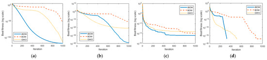
Figure 7.
Average convergence curves of benchmark test functions: (a) F1 function; (b) F4 function; (c) F7 function; (d) F11 function.
4. Results
4.1. Model Performance Comparison Experiments
To evaluate the effectiveness of the proposed ground-type recognition model based on the 1D-CNN-LSTM-CBAM architecture and the improved Whale Optimization Algorithm (iBWOA), five comparative experiments with different network architectures were designed and conducted.
The detailed configurations of each comparative model are summarized in Table 1.

Table 1.
Architectural configurations of different models.
To comprehensively evaluate the model performance, four standard classification metrics were employed: Accuracy, Precision, Recall, and F1-score.
Accuracy measures the proportion of correctly classified samples among all samples. The formula is as follows:
where TP is the number of samples predicted to be positive and actually positive, FP is the number of samples predicted to be positive but actually negative, FN is the number of samples predicted to be negative but actually positive, TN is the number of samples predicted to be negative and actually negative.
Precision represents the proportion of correctly predicted positive samples among all samples predicted as positive. The formula is as follows:
Recall measures the proportion of correctly predicted positive samples among all actual positive samples. The formula is as follows:
F1-score is the harmonic mean of Precision and Recall. The formula is as follows:
Based on the above four metrics, the classification performance of the five comparative models was quantitatively analyzed. The experimental results are presented in Table 2, from which it can be observed that the classification performance consistently improves with the progressive optimization of the model architecture. Among them, the 1D-CNN-LSTM-CBAM + iBWOA model achieved the best performance in terms of Accuracy, Precision, Recall, and F1-score, fully demonstrating the effectiveness and superiority of the proposed model in the terrain type recognition task.
Table 2.
Classification performance metrics of different models.
To further evaluate the performance of the models on specific terrain classification tasks, confusion matrices were constructed to visually present the classification results for each category. Based on these results, the corresponding classification performance metrics were calculated. Figure 8 presents the visualization of confusion matrices for different classification models, while Table 3 summarizes the classification performance metrics of each model across various terrain types.
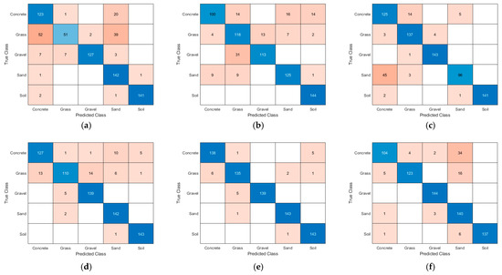
Figure 8.
Confusion matrix plot of different models: (a) 1D-CNN; (b) 1D-CNN-LSTM; (c) 1D-CNN-LSTM-CBAM; (d) 1D-CNN-LSTM-CBAM + BWOA; (e) 1D-CNN-LSTM-CBAM + iBWOA; (f) TRANSFORMER.
Table 3.
Classification Performance of Different Models on Various Terrain Types.
As shown in Figure 8 and Table 3, the proposed 1D-CNN-LSTM-CBAM-iBWOA model exhibits excellent and relatively balanced recognition performance across all ground categories, achieving an overall classification accuracy of 96.94%. For “Cement,” “Gravel,” “Soil,” and “Sand,” the precision, recall, and F1-scores all exceed 95%, with “Cement” and “Gravel” demonstrating particularly strong discriminability in the high-dimensional feature space. The “Sand” category achieves both precision and recall above 0.95973, indicating stable recognition capability. While the “Soil” category presents some challenges in boundary sample discrimination, it still maintains 95.83% precision and recall. In comparison, the “Grass” category shows slightly lower precision (95.07%), primarily due to the similarity of its contact mechanical properties with “Soil,” leading to minor cross-misclassifications in the confusion matrix. Overall, the proposed model effectively captures subtle differences in triaxial force sensing signals across various ground types and maintains high discriminative capability even between categories with similar contact characteristics, demonstrating excellent generalization and robustness.
4.2. Feature Visualization Analysis
To gain deeper insights into the internal discriminative capability of the models, the t-distributed stochastic neighbor embedding (t-SNE) technique was employed to project the high-dimensional features extracted by the models onto a two-dimensional space for intuitive visualization. Figure 9 illustrates the distribution of high-dimensional features from different models in the two-dimensional space.
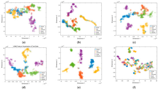
Figure 9.
t-SNE visualization of the high-dimensional features extracted by different models: (a) 1D-CNN; (b) 1D-CNN-LSTM; (c) 1D-CNN-LSTM-CBAM; (d) 1D-CNN-LSTM-CBAM + BWOA; (e) 1D-CNN-LSTM-CBAM + iBWOA; (f) TRANSFORMER.
Table 4 presents the global evaluation metrics of the model, which are defined as follows.
Table 4.
Global evaluation metrics of the model.
Trustworthiness measures whether spurious neighborhood relationships are introduced in the low-dimensional space. If two points that are not neighbors in the high-dimensional space are incorrectly mapped as neighbors in the low-dimensional embedding, the trustworthiness decreases. A higher value indicates that the low-dimensional embedding more reliably preserves the neighborhood structure of the high-dimensional space.
Continuity evaluates whether the neighborhood relationships in the high-dimensional space are preserved in the low-dimensional embedding. If neighbors in the high-dimensional space are not retained as neighbors in the low-dimensional space, the continuity decreases. A higher value implies that the low-dimensional embedding better maintains the structural continuity of the original high-dimensional data.
Silhouette Coefficient is employed to evaluate the clustering quality after dimensionality reduction. For each sample , its silhouette value is computed based on the mean intra-cluster distance and the mean nearest-cluster distance , as follows:
The overall silhouette coefficient is defined as the average silhouette value across all samples:
where denotes the total number of samples. The value of lies within [−1, 1]. A value close to 1 indicates that samples are well clustered with high intra-cluster compactness and clear inter-cluster separation. A value around 0 suggests overlapping clusters with ambiguous boundaries, while negative values imply that some samples may have been incorrectly assigned to inappropriate clusters.
Intra-/Inter-cluster Distance Ratio is employed to assess the compactness and separability of clustering results. The core principle is that better clustering corresponds to smaller intra-cluster distances and larger inter-cluster distances. The definitions are as follows.
Intra-cluster distance :
Inter-cluster distance :
Intra-/Inter-cluster Distance Ratio :
where denotes the number of cluster, represents the k-th cluster, and is the centroid of cluster .
As shown in the t-SNE visualization results in Figure 9 and the global evaluation metrics in Table 4, different models exhibit substantially different clustering behaviors in the high-dimensional feature space. With the progressive enhancement of model architectures, the feature distribution evolves from dispersed and ambiguous clusters to more compact intra-class structures and clearer inter-class separation. Among all models, the proposed 1D-CNN-LSTM-CBAM-iBWOA achieves the most distinct clustering performance, where the five ground categories form well-defined clusters with almost no noticeable misclassification. Consistently, this model also delivers the best results across global evaluation metrics, with trustworthiness and continuity both equal to 1, a silhouette coefficient of 0.76192, and an intra-/inter-cluster distance ratio of 0.25814. These results confirm the effectiveness and robustness of the proposed model for ground type recognition tasks.
In contrast, although the Transformer model achieves near-optimal continuity, its negative silhouette coefficient indicates poor clustering quality and insufficient inter-class separability. Its reported classification accuracy of approximately 91% may largely be attributed to overfitting, where the model memorizes ambiguous or mislabeled training samples rather than learning generalizable patterns. As a result, while it appears to perform well on the training data, its generalization capability on unseen samples is considerably limited, suggesting that the seemingly high accuracy does not truly reflect reliable recognition performance in complex terrain scenarios.
5. Conclusions
This paper proposes a ground-type recognition method for legged robots based on single-foot triaxial force signals, integrating 1D-CNN, LSTM, and the CBAM attention mechanism to fully exploit temporal dependencies, key channel information, and local spatial features. Furthermore, the improved Beluga Whale Optimization Algorithm (iBWOA) is introduced to perform global automated tuning of key hyperparameters, including the number of convolutional kernels, LSTM units, and dropout rate, thereby balancing feature extraction capability and model generalization. The experimental results show that the proposed method achieves an overall classification accuracy of 96.94% across five representative ground types—grass, cement, gravel, soil, and sand—under multiple slope and force conditions, with high precision, recall, and F1-scores for all classes. t-SNE feature visualization and confusion matrix analysis further confirm that the proposed model exhibits strong intra-class compactness and inter-class separability in high-dimensional feature space, significantly reducing misclassification between categories. In summary, the proposed method maintains excellent discriminative power and stability across different ground types, providing a high-accuracy and robust perception framework for legged robots in real-world complex environments. Future work will focus on incorporating multi-modal sensor fusion and cross-domain transfer learning to further enhance generalization and stability in extreme and dynamic scenarios.
Author Contributions
Methodology, Y.L. and R.S.; software, Y.L., X.T. and R.S.; validation, Y.L., X.T., R.S. and T.S.; formal analysis, R.S. and Y.L.; investigation, Y.L., X.T., T.S. and T.H.; data curation, R.S., X.T. and T.S.; writing—original draft preparation, Y.L. and R.S.; writing—review and editing, Y.L., R.S., X.T. and T.S.; visualization, Y.L. and T.H.; supervision, Y.L. and R.S.; project administration, Y.L.; funding acquisition, Y.L. All authors have read and agreed to the published version of the manuscript.
Funding
This research was funded by the Science and Technology Bureau of Luzhou City, Sichuan Province, with the project approval number being 2024RQN214.
Institutional Review Board Statement
Not applicable.
Data Availability Statement
The data can be obtained from the authors, but the specific data of the article relates to pit-specific parameters and is not available to the public.
Conflicts of Interest
The authors declare no conflicts of interest. The funders had no role in the design of the study; in the collection, analyses, or interpretation of data; in the writing of the manuscript; or in the decision to publish the results.
References
- Cheng, L.; Zhang, X.; Shen, J. Road surface condition classification using deep learning. J. Vis. Commun. Image Represent. 2019, 64, 102638. [Google Scholar] [CrossRef]
- Šabanovič, E.; Žuraulis, V.; Prentkovskis, O.; Skrickij, V. Identification of road-surface type using deep neural networks for friction coefficient estimation. Sensors 2020, 3, 612. [Google Scholar] [CrossRef] [PubMed]
- Laschowski, B.; McNally, W.; Wong, A.; McPhee, J. Environment classification for robotic leg prostheses and exoskeletons using deep convolutional neural networks. Front. Neurorobotics 2022, 15, 730965. [Google Scholar] [CrossRef] [PubMed]
- Chen, H.-Y.; Sang, I.-C.; Norris, W.R.; Soylemezoglu, A.; Nottage, D. Terrain classification method using an NIR or RGB camera with a CNN-based fusion of vision and a reduced-order proprioception model. Comput. Electron. Agric. 2024, 227, 109539. [Google Scholar] [CrossRef]
- Pešek, O. Možnosti Využití Konvolučních Neuronových Sítí Pro Obrazovou Klasifikaci V Dálkovém Průzkumu Země. Diss. Ph.D. Thesis, Czech Technical University, Prague, Czech Republic, 2024. [Google Scholar]
- Jiang, J.; Xu, G.; Wang, H.; Yang, Z.; Sun, B.; Guan, C.; Feng, J.; Ma, Y.; Chen, X. High-accuracy road surface condition detection through multi-sensor information fusion based on WOA-BP neural network. Sens. Actuators A Phys. 2024, 378, 115829. [Google Scholar] [CrossRef]
- Wu, X.A.; Huh, T.M.; Sabin, A.; Suresh, S.A.; Cutkosky, M.R. Tactile sensing and terrain-based gait control for small legged robots. IEEE Trans. Robot. 2019, 1, 15–27. [Google Scholar] [CrossRef]
- Mei, M.; Chang, J.; Li, Y.; Li, Z.; Li, X.; Lv, W. Comparative study of different methods in vibration-based terrain classification for wheeled robots with shock absorbers. Sensors 2019, 5, 1137. [Google Scholar] [CrossRef] [PubMed]
- Bai, C.; Guo, J.; Guo, L.; Song, J. Deep multi-layer perception based terrain classification for planetary exploration rovers. Sensors 2019, 14, 3102. [Google Scholar] [CrossRef] [PubMed]
- Vulpi, F.; Milella, A.; Marani, R.; Reina, G. Recurrent and convolutional neural networks for deep terrain classification by autonomous robots. J. Terramechanics 2021, 96, 119–131. [Google Scholar] [CrossRef]
- Wang, M.; Ye, L.; Sun, X. Adaptive online terrain classification method for mobile robot based on vibration signals. Int. J. Adv. Robot. Syst. 2021, 6, 17298814211062035. [Google Scholar] [CrossRef]
- Bednarek, M.; Nowicki, M.R.; Walas, K. HAPTR2: Improved Haptic Transformer for legged robots’ terrain classification. Robot. Auton. Syst. 2022, 158, 104236. [Google Scholar] [CrossRef]
- Ugenti, A.; Vulpi, F.; Domínguez, R.; Cordes, F.; Milella, A.; Reina, G. On the role of feature and signal selection for terrain learning in planetary exploration robots. J. Field Robot. 2022, 4, 355–370. [Google Scholar] [CrossRef]
- Lv, F.; Li, N.; Gao, H.; Ding, L.; Deng, Z.; Yu, H.; Liu, Z. Vibration-Based Recognition of Wheel–Terrain Interaction for Terramechanics Model Selection and Terrain Parameter Identification for Lugged-Wheel Planetary Rovers. Sensors 2023, 24, 9752. [Google Scholar] [CrossRef] [PubMed]
- Sarcevic, P.; Csík, D.; Pesti, R.; Stančin, S.; Tomažič, S.; Tadic, V.; Rodriguez-Resendiz, J.; Sárosi, J.; Odry, A. Online outdoor terrain classification algorithm for wheeled mobile robots equipped with inertial and magnetic sensors. Electronics 2023, 15, 3238. [Google Scholar] [CrossRef]
- Zhang, Y.; Huang, B.; Hong, M.; Huang, C.; Wang, G.; Guo, M. A Terrain Classification Method for Quadruped Robots with Proprioception. Electronics 2025, 6, 1231. [Google Scholar] [CrossRef]
- Halatci, I.; Brooks, C.A.; Iagnemma, K. A study of visual and tactile terrain classification and classifier fusion for planetary exploration rovers. Robotica 2008, 6, 767–779. [Google Scholar] [CrossRef]
- Yu, C.; Rastogi, C.; Norris, W.R. A cnn based vision-proprioception fusion method for robust ugv terrain classification. IEEE Robot. Autom. Lett. 2021, 4, 7965–7972. [Google Scholar] [CrossRef]
- Haddeler, G.; Chuah, M.Y.; You, Y.; Chan, J.; Adiwahono, A.H.; Yau, W.Y.; Chew, C.-M. Traversability analysis with vision and terrain probing for safe legged robot navigation. Front. Robot. AI 2022, 9, 887910. [Google Scholar] [CrossRef] [PubMed]
- Wang, H.; Lu, E.; Zhao, X.; Xue, J. Vibration and image texture data fusion-based terrain classification using WKNN for tracked robots. World Electr. Veh. J. 2023, 8, 214. [Google Scholar] [CrossRef]
- Prágr, M.; Bayer, J.; Faigl, J. Autonomous exploration with online learning of traversable yet visually rigid obstacles. Auton. Robot. 2023, 2, 161–180. [Google Scholar] [CrossRef]


Disclaimer/Publisher’s Note: The statements, opinions and data contained in all publications are solely those of the individual author(s) and contributor(s) and not of MDPI and/or the editor(s). MDPI and/or the editor(s) disclaim responsibility for any injury to people or property resulting from any ideas, methods, instructions or products referred to in the content. |
© 2025 by the authors. Licensee MDPI, Basel, Switzerland. This article is an open access article distributed under the terms and conditions of the Creative Commons Attribution (CC BY) license (https://creativecommons.org/licenses/by/4.0/).