Active Control Method for Pantograph-Catenary System Based on Neural Network PID Under Crosswind Conditions

Abstract

Crosswind is a critical environmental factor affecting the dynamic interaction between the pantograph and catenary in high-speed trains, which can severely compromise the operational stability of the system. To address this challenge, this study develops an active pantograph control scheme for crosswind disturbances by employing a neural network-based PID controller. First, the target value is determined based on the train operating speed and inherent data of the pantograph-catenary system, and a PID controller is constructed. Subsequently, a neural network is integrated into the controller to train the system’s output contact force and PID parameters using its nonlinear approximation capability, thereby optimizing the parameters and achieving effective control of the system. The effectiveness of the controller is then validated by applying the proposed method to a high-speed train pantograph-catenary system under crosswind conditions, with its control performance thoroughly analyzed. The results indicate that the proposed control scheme demonstrates effective regulation of the pantograph-catenary system across various typical crosswind scenarios, achieving significant reduction or even complete elimination of pantograph-catenary’s contact loss rate while exhibiting strong robustness, thereby proving fully applicable for practical implementation in high-speed railway engineering applications.

1. Introduction

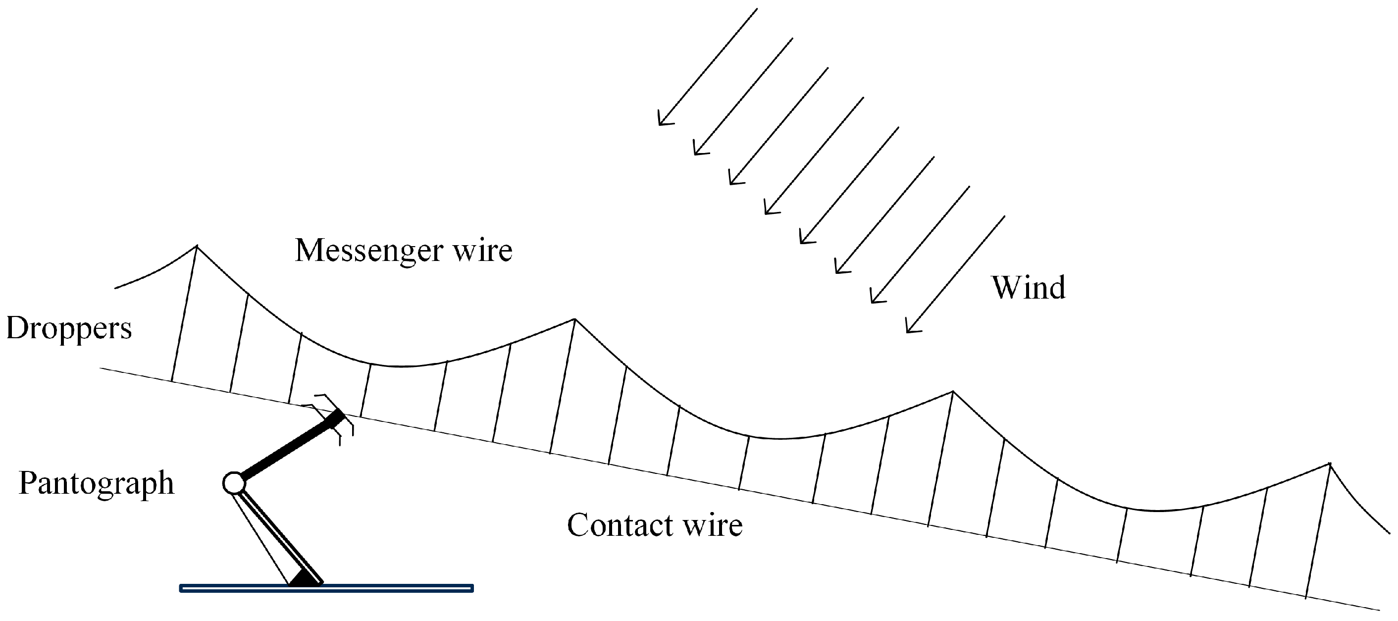
As a critical component of electrified railways, the stable contact of the pantograph-catenary system ensures the operational reliability of railway systems. However, with the increasing frequency of extreme weather events worldwide, crosswinds acting on overhead contact lines have become more intense, thereby compromising the stability of the pantograph-catenary system (As illustrated in Figure 1). Statistical data reveal numerous instances of wind-induced train service suspensions. For example, Train L656 on the Lanzhou-Xinjiang Railway was forced to stop due to strong winds, causing a cascading delay of nearly 7.5 h for subsequent trains. Improving the dynamic response characteristics of the pantograph-catenary system under crosswind conditions is essential for enhancing the operational stability of electrified railways and effectively mitigating the risks of service interruptions caused by routine crosswinds.

Extensive research has been conducted by scholars worldwide on the contact performance of pantograph-catenary systems under crosswind conditions. Some scholars have investigated the effects of crosswind speed, angle of attack, and turbulence intensity on the pantograph-catenary system by establishing wind field models. The results demonstrate that these factors exacerbate the vibration of the catenary, significantly impairing the current collection stability of the system and posing a serious threat to train operational safety [1,2,3,4]. Luo et al. [5] established a pantograph-catenary coupled system using the absolute nodal coordinate formulation (ANCF) and relevant standards, demonstrating that contact force fluctuations intensify with increasing wind speed. Niu and Zhou [6] examined crosswind effects on pantograph heads during tunnel entry and exit, identifying stronger dynamic responses during exit phases. Daocharoenporn and Mongkolwongrojn [7] employed multibody system (MBS) dynamics to simulate wear mechanisms, correlating increased wind speed with elevated contact wire wear and separation rates. Li et al. [8] analyzed lateral displacement under crosswind effects using a proposed prediction model and conducted a contact stability analysis. Xie and Zhi [9] used sensor arrays to collect measurement-point data and examined wind effects on the catenary through wind tunnel experiments. Numerical simulations revealed significant displacement of the catenary under wind loads, adversely affecting the contact stability of the coupled pantograph-catenary system. Pan et al. [10] evaluated dropper fatigue life via MATLAB R2023a, linking crosswinds to accelerated wear. Duan et al. [11] characterized contact wires with varying wear levels under wind loads and proposed design improvements. Chen et al. [12] established wind fields to analyze fluctuation velocities, demonstrating that pulsation intensity is proportional to contact wire impacts. Based on the aforementioned findings, it can be concluded that crosswinds exert significant adverse effects on the operational stability of pantograph-catenary systems.

Compared with studies investigating the current collection performance of pantograph-catenary systems under crosswinds, relatively limited research has focused on maintaining and improving such performance under crosswind conditions. Song et al. [13] developed a nonlinear catenary model and a multibody dynamic pantograph model, and proposed a control strategy using a PD controller with different actuator configurations. The reliability of the approach was validated under strong wind conditions. Addressing stochastic wind fields, Song et al. [14] introduced an active pantograph control strategy based on PD sliding-mode surfaces, which effectively suppresses contact force fluctuations by reducing the pantograph head’s mechanical impedance. Ren et al. [15] applied sliding-mode control to a three-mass pantograph model under pulsating wind loads, achieving significant vibration suppression and a reduced standard deviation of contact forces. For transitional windbreak wall zones, Zhang et al. [16] proposed a localized optimization approach to counteract train yaw effects. Dong et al. [17] enhanced catenary performance by installing porous wind barriers on top of embankment windbreak walls. Their parametric study on porosity ratios revealed that optimal porosity configurations can effectively minimize conductor displacement. However, these studies predominantly rely on infrastructure-based methodologies and conventional control strategies.

In recent years, an increasing number of studies have applied advanced control strategies to nonlinear systems, such as state-filtering-based disturbance rejection control [18] and multi-layer neural control strategies [19]. However, due to issues such as potential high-frequency noise in the pantograph–catenary system itself and substantial computational demands, these methods exhibit certain limitations. Neural network-based PID control has been widely applied in the field of active suspension systems. Some studies have introduced disturbances to simulate road unevenness and utilized neural network PID controllers to optimize suspension performance [20,21]. Duan et al. [22] employed an improved neural network PID strategy to enhance the performance of a passive suspension model under various road conditions. Liu et al. [23] optimized vehicle performance indicators using a proposed BP-PID control method and validated its superiority through comparison with conventional PID approaches. Effendi et al. [24] developed a PID tuning method based on a backpropagation neural network combined with a genetic algorithm to improve ride comfort, demonstrating its effectiveness through computed metrics and relevant evaluation standards. However, research on the application of neural network PID control to pantograph-catenary systems under crosswind conditions remains relatively limited.

As evidenced by the aforementioned research, while active control methods represent an effective approach for improving the current collection performance of pantograph-catenary systems under crosswind conditions, current studies still exhibit certain limitations. Firstly, the catenary models employed are often oversimplified; secondly, existing active control strategies tend to be overly complex, making them difficult to implement in practical pantograph systems. To better enhance the current collection quality of high-speed railway pantograph-catenary systems under crosswind effects, this paper adopts an offline and online combined neural network-based PID strategy within the MATLAB environment for system control. Owing to the hybrid offline-online nature of the proposed method, a feedback structure is utilized in this study. Given that PID control is most likely to be implemented in practical pantograph-catenary applications and considering the inherent capabilities of Radial Basis Function (RBF) networks, the proposed framework employs a PID controller with RBF-based algorithm parameter adjustment.

This study proposes a neural network-based PID control approach for the pantograph-catenary system to optimize current collection quality under crosswind disturbances. First, models of the pantograph, catenary, and crosswind are established. A simplified stitched catenary model is formulated using the Lagrange equation, while the pantograph is modeled as a two-mass block system. The coupling relationship between the pantograph and catenary is then established via the penalty function method, forming a complete pantograph-catenary system into which the crosswind effect is incorporated. Subsequently, the contact quality is optimized using a neural network PID method, with contact force selected as the feedback variable and the output lifting force controlled through the proposed strategy. By selecting appropriate initial values for the proportional-integral-derivative (PID) controller and initializing learning rates as well as weight coefficients, effective system control is achieved with favorable results. Section 2 develops the pantograph–catenary interaction model based on the derived dynamic equations, incorporating crosswind models at varying wind speeds; Section 3 constructs the neural network PID control framework; Section 4 analyzes the control outcomes, with comparative validation demonstrating the effectiveness of the proposed method; Section 5 presents the conclusions.

2. Pantograph-Catenary Interaction System Model Under Crosswind Conditions

Establishing a pantograph-catenary coupled dynamic model considering crosswind effects is fundamental to investigating its active control strategies (as illustrated in Figure 2). The reduced pantograph-catenary model was employed to establish a high-speed railway pantograph-catenary interaction model. By incorporating established crosswind models into this coupled dynamic system, the analysis of interaction behavior under crosswind conditions was achieved. The specific modeling procedure is detailed below.

2.1. Catenary Model

This study adopts a simple stitched catenary for investigation, the structure of which primarily consists of a contact wire, droppers, and a messenger wire, as illustrated in Figure 2. A nonlinear catenary model capable of accurately reflecting the system’s dynamic characteristics was established using the modal superposition method. Relevant parameters are detailed in

Table 1. Catenary system parameters.

Parameter	$\mathbf{Density}/\mathbf{k}\mathbf{g}\cdot {\mathbf{m}}^{-3}$	Young’s Modulus/Pa	Shear Modulus/Pa	Cross-Sectional Area/m2	Torsional Inertia/m4	Tension/N
Contact wire	8920	1.2 × 1011	0.46 × 1011	1 × 10−4	17.4402 × 10−10	15,800
Messenger wire	8920	1.2 × 1011	0.46 × 1011	0.5 × 10−4	7.4402 × 10−10	8600

[25].

According to [26], the contact wire and messenger wire are modeled as Euler-Bernoulli beams, whose kinetic energy expressions can be formulated as follows:

$$T_m={\displaystyle \frac{1}{2}}{\displaystyle \underset{\Omega }{\int }{\rho }_m{{\dot{y}}_m}^2\mathrm{d}\Omega }+{\displaystyle \frac{1}{2}}{\displaystyle \underset{\Omega }{\int }{\rho }_m{{\dot{z}}_m}^2\mathrm{d}\Omega }+{\displaystyle \frac{1}{2}}{\displaystyle \underset{\Omega }{\int }{\rho }_m\left({y_m}^2+{z_m}^2\right){{\dot{\varphi }}_m}^2\mathrm{d}\Omega }$$

(1)

$$T_c={\displaystyle \frac{1}{2}}{\displaystyle \underset{\Omega }{\int }{\rho }_c{{\dot{y}}_c}^2\mathrm{d}\Omega }+{\displaystyle \frac{1}{2}}{\displaystyle \underset{\Omega }{\int }{\rho }_c{{\dot{z}}_c}^2\mathrm{d}\Omega }+{\displaystyle \frac{1}{2}}{\displaystyle \underset{\Omega }{\int }{\rho }_c\left({y_c}^2+{z_c}^2\right){{\dot{\varphi }}_c}^2\mathrm{d}\Omega }$$

(2)

where $\rho$ represents the beam density; the lateral displacement, vertical displacement, and rotation about the central axis of the beam cross-section are expressed as y, z, and $\varphi$, respectively. The messenger wire and contact wire indicated by the subscripts m and c, respectively, and the dot notation denotes differentiation with respect to time. $\mathrm{d}\Omega$ is the volume integral.

The strain energy of the contact wire and messenger wire is given by Equations (3) and (4), as follows [26]:

$$\begin{array}{l}{U}_m={\displaystyle \frac{1}{2}}{\displaystyle {\int }_0^l{E}_m{I}_{ym}}{\left(z_m^{″}\right)}^2\mathrm{d}x+{\displaystyle \frac{1}{2}}{\displaystyle {\int }_0^l{E}_m{I}_{zm}}{\left(y_m^{″}\right)}^2\mathrm{d}x+{\displaystyle \frac{1}{2}}{\displaystyle {\int }_0^l{G}_m{I}_{{\varphi }_m}}{\left({\varphi }_m^{\prime }\right)}^2\mathrm{d}x\\ \hspace{0.33em}\hspace{0.33em}\hspace{0.33em}+{\displaystyle \frac{1}{2}}{\displaystyle {\int }_0^l{T}_{sm}}{\left(y_m^{\prime }\right)}^2\mathrm{d}x+{\displaystyle \frac{1}{2}}{\displaystyle {\int }_0^l{T}_{sm}}{\left(z_m^{\prime }\right)}^2\mathrm{d}x\end{array}$$

(3)

$$\begin{array}{l}{U}_c={\displaystyle \frac{1}{2}}{\displaystyle {\int }_0^l{E}_c{I}_{yc}}{\left(z_c^{″}\right)}^2\mathrm{d}x+{\displaystyle \frac{1}{2}}{\displaystyle {\int }_0^l{E}_c{I}_{zc}}{\left(y_c^{″}\right)}^2\mathrm{d}x+{\displaystyle \frac{1}{2}}{\displaystyle {\int }_0^l{G}_c{I}_{\varphi c}}{\left({\varphi }_c^{\prime }\right)}^2\mathrm{d}x\\ \hspace{0.33em}\hspace{0.33em}\hspace{0.33em}+{\displaystyle \frac{1}{2}}{\displaystyle {\int }_0^l{T}_{\mathit{sc}}}{\left(y_c^{\prime }\right)}^2\mathrm{d}x+{\displaystyle \frac{1}{2}}{\displaystyle {\int }_0^l{T}_{sc}}{\left(z_c^{\prime }\right)}^2\mathrm{d}x\end{array}$$

(4)

where E and G represent the Young’s modulus and shear modulus of the beam, respectively; the moment of inertia of the beam cross-section about the y-axis, z-axis, and torsional axis are denoted as $I_y$, $I_z$, and $I_{\varphi }$, respectively; $T_s$ represents the tension in the beam; the notations ${(\cdot )}^{’}$ and ${(\cdot )}^{’’}$ denote the first- and second-order partial derivatives with respect to x, respectively. According to [26], in Equations (1)–(4), the variables y, z, and x are expressed by Equations (5) and (6).

$$y_m(x,t)=Y_m(x)q_{my}(t), z_m(x,t)=Z_m(x)q_{mz}(t), {\varphi }_m(x,t)={\Phi }_m(x)q_{mx}(t)$$

(5)

$$y_c(x,t)=Y_c(x)q_{cy}(t), z_c(x,t)=Z_c(x)q_{cz}(t), {\varphi }_c(x,t)={\Phi }_c(x)q_{cx}(t)$$

(6)

where $Y, Z, \Phi$ represents the shape function; $q$ denotes the generalized coordinate vector. The modal superposition method simplifies the structural response into a linear combination of shape functions and generalized coordinates by introducing shape functions, thereby decomposing the model into a superposition of multiple simple modes. This approach enables modal decomposition of the model, improving computational efficiency and facilitating the construction of catenary models.

The expression for the force generated by the dropper in the catenary model is given by [26]:

$$F_d=K_d{d}_i$$

(7)

where $K_d$ represents the dropper stiffness, and $d_i$ denotes the relative displacement between the contact wire and messenger wire.

Based on the aforementioned kinetic energy, strain energy, and related expressions, the dynamic equations for the contact wire and messenger wire are derived as follows [26]:

$$M_m{\ddot{q}}_m+C_m{\dot{q}}_m+K_m{q}_m=Q_m$$

(8)

$$M_c{\ddot{q}}_c+C_c{\dot{q}}_c+K_c{q}_c=Q_c$$

(9)

where M is the mass matrix, C is the damping matrix, and K is the stiffness matrix; Q represents the generalized force, which includes the dropper force, the gravitational forces of the messenger wire and contact wire, as well as the suspension force. The detailed expressions of these matrices can be seen in [26].

2.2. Pantograph Model

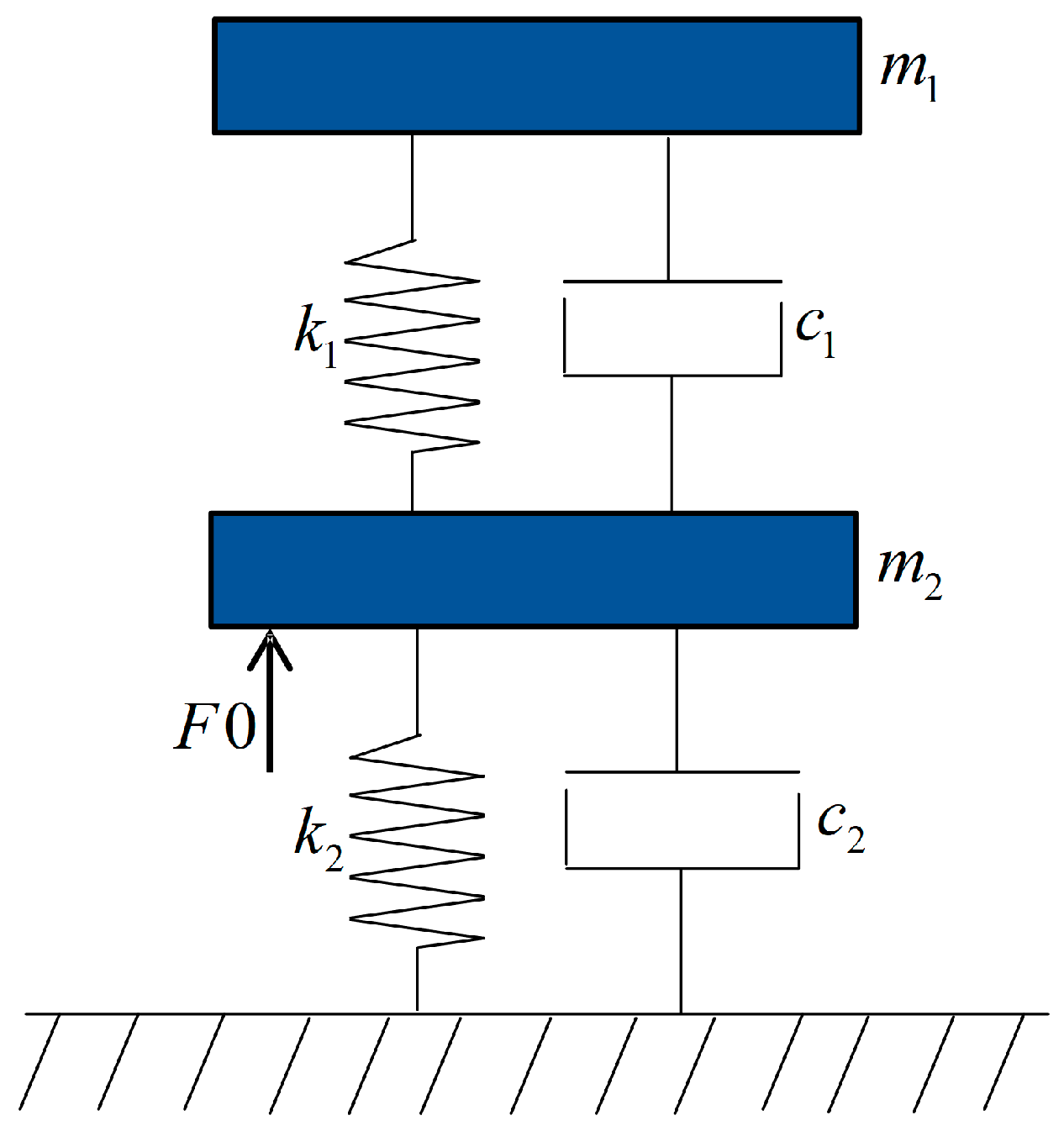
As a vital component of the pantograph-catenary system, the pantograph plays a crucial role in powering trains by collecting electricity through contact with the catenary, thereby enabling vehicle propulsion. Research on current collection systems predominantly employs lumped-mass pantograph models, specifically two-mass and three-mass configurations. Since this study primarily focuses on the impact of crosswinds on the catenary system, with minimal influence on the pantograph, the two-mass model—despite providing a simplified structural representation compared to nonlinear pantograph models—effectively captures the dynamic characteristics of the pantograph. Accordingly, this study adopts the lumped-mass modeling approach, implementing a two-degree-of-freedom pantograph model using MATLAB numerical simulation platform [25] (as shown in Figure 3). The system configuration comprises a pantograph head (mass $m_1$) and a pantograph frame (mass $m_2$), mechanically coupled through spring ($k_1$, $k_2$) and damper ($c_1$, $c_2$) elements, with the frame mounted to the vehicle body. The static uplift force F0 is maintained at 50 N throughout simulations. In compliance with standards for high-speed operation (≥200 km/h), the target contact force is calculated as follows:

$$F=50 + 0.00097V^2$$

(10)

The pantograph dynamic equation is formulated as follows [26]:

$$M_p{\ddot{q}}_p+C_p{\dot{q}}_p+K_p{q}_p=Q_{cp}+Q_p$$

(11)

where $M_p$ represents the pantograph mass; $C_p$ represents the pantograph stiffness; $K_p$ represents the pantograph damping coefficient; $Q_{cp}$ is the contact force; $Q_p$ representing the aerodynamic uplift force and static uplift force, respectively. The expression of the matrices in Equation (11) can be found in [25].

2.3. Crosswind Model

Under crosswind conditions, both the static and dynamic characteristics of the catenary undergo modifications, consequently affecting the pantograph-catenary coupled dynamics. By establishing a crosswind model, the generalized wind-induced forces can be derived and incorporated into the pantograph-catenary system model, enabling a comprehensive investigation of the wind-affected current collection performance. Figure 4 illustrates the catenary model subjected to crosswind excitation.

The present study establishes a crosswind model based on stochastic wind field theory, in which the stochastic wind field primarily consists of mean wind and fluctuating wind components. Currently, the most widely used stochastic wind field models in domestic and international research are power spectral density formulations, including the Davenport spectrum, Kaimal spectrum, and Von Karman spectrum [27]. Among these, the Davenport spectrum has been extensively applied in crosswind analysis of overhead contact lines. Therefore, this study employs the Davenport spectrum to simulate crosswind effects on the contact line. The Davenport spectrum [27], proposed by A. G. Davenport in 1961, characterizes the frequency-dependent variation in turbulent wind velocity in natural wind fields. Its mathematical expression is given by:

$$S_u\left(f\right)={\displaystyle \frac{4K{U}^2}{f}}·{\displaystyle \frac{X^2}{{\left(1+X^2\right)}^{4/3}}}$$

(12)

where $S_u\left(f\right)$ represents the wind speed spectral density; f denotes the frequency of wind speed fluctuations; K denotes the surface roughness coefficient, dependent on terrain characteristics; U indicates the mean wind speed at the given location; dimensionless parameter $X={\displaystyle \frac{1200f}{U}}$. Based on this stochastic wind field power spectrum, the frequency distributions of wind fields corresponding to different mean wind speeds can be derived. Subsequently, by further transforming the spectrum and employing the spectral representation method, the following can be derived:

$$u\left(t\right)={\displaystyle \sum _{n=1}^N\sqrt{2S_u\left(f_n\right)\Delta f}}\cos \left(2\pi f_{n}t+{\varphi }_n\right)$$

(13)

where N denotes the number of frequency steps; $\Delta f$ represents the frequency interval; ${\varphi }_n$ represents the stochastic phase angle. Using the above formulation, the stochastic wind field spectral density and corresponding time-history curves can be computed for various wind speeds. Figure 5 displays the stochastic wind speed spectra and corresponding time-history curves under different wind speed levels.

According to the principles of fluid dynamics, the specific calculation formula for the wind force acting on an object is [28]:

$$F\left(t\right)={\displaystyle \frac{1}{2}}\rho C_{d}Au{\left(t\right)}^2$$

(14)

where $\rho$ denotes the air density, $C_d$ represents the air damping coefficient, and A stands for the windward projected area of the object.

Further considering the influence of fluctuating wind, the wind speed can be decomposed into the mean wind speed U and the fluctuating wind speed $u^{\prime }\left(t\right)$. Accordingly, Equation (14) can be further derived as:

$$F\left(t\right)={\displaystyle \frac{1}{2}}\rho C_{d}A{\left(U+u^{\prime }\left(t\right)\right)}^2$$

(15)

Expanding the equation yields:

$$F\left(t\right)={\displaystyle \frac{1}{2}}\rho C_{d}A\left(U^2+2U{u}^{\prime }\left(t\right)+u^{\prime }{\left(t\right)}^2\right)$$

(16)

Since the fluctuating wind speed is typically negligible, Equation (16) can be simplified as:

$$F\left(t\right)={\displaystyle \frac{1}{2}}\rho C_{d}A\left(U^2+2U{u}^{\prime }\left(t\right)\right)$$

(17)

Ultimately, the expression for the wind-induced force acting on the structure under stochastic wind field conditions can be formulated as:

$$F\left(t\right)={\displaystyle \frac{1}{2}}\rho C_{d}A{U}^2+\rho C_{d}AU{u}^{\prime }\left(t\right)$$

(18)

The above stochastic wind field force is imported to establish a pantograph-catenary coupled dynamics model under crosswind conditions. Since the crosswind acts as a distributed load on a continuous structure, the generalized force expression is as follows:

$$Q_w={\displaystyle {\int }_0^{l}F\left(t\right)}N\left(x\right)dx$$

(19)

where N represents the shape function.

2.4. Coupled Pantograph-Catenary Model Under Crosswind Conditions

The final coupled dynamics equations of the pantograph-catenary system under crosswind excitation are derived from Equations (8), (9) and (11). The detailed derivation process and the definitions of parameters within the matrices can be found in [26]. The relevant parameters in the matrices are provided in Table 1 and

Table 2. Pantograph parameters.

Parameter	Value
$m_1$	6.6 kg
$c_1$	75.6 $\mathrm{N}\cdot \mathrm{s}\cdot {\mathrm{m}}^{-1}$
$k_1$	2200 $\mathrm{N}\cdot {\mathrm{m}}^{-1}$
$m_2$	5.56 kg
$c_2$	63.5 $\mathrm{N}\cdot \mathrm{s}\cdot {\mathrm{m}}^{-1}$
$k_2$	1,000,000 $\mathrm{N}\cdot {\mathrm{m}}^{-1}$
$F0$	50 N

.

$$\left[\begin{array}{ccc}{M}_m& 0& 0\\ 0& M_c& 0\\ 0& 0& M_P\end{array}\right]\left[\begin{array}{c}{\ddot{q}}_m\\ {\ddot{q}}_c\\ {\ddot{q}}_p\end{array}\right]+\left[\begin{array}{ccc}{C}_m& 0& 0\\ 0& C_c& 0\\ 0& 0& C_P\end{array}\right]\left[\begin{array}{c}{\dot{q}}_m\\ {\dot{q}}_{\mathrm{c}}\\ {\dot{q}}_p\end{array}\right]+\left[\begin{array}{ccc}{K}_m& 0& 0\\ 0& K_c& 0\\ 0& 0& K_P\end{array}\right]\left[\begin{array}{c}{q}_m\\ q_c\\ q_p\end{array}\right]=\left[\begin{array}{c}{Q}_m+Q_w\\ Q_c+Q_{pc}+Q_w\\ Q_{cp}+Q_p\end{array}\right]$$

(20)

where $Q_{cp}$ represents the contact force.

In the calculation of contact forces, the displacement and velocity at the zero-state are input as initial conditions. The coupled pantograph-catenary dynamic equations are then solved using MATLAB’s ode15s solver, yielding displacement and velocity solutions from time zero to the current step. These solutions subsequently serve as initial conditions for the next step’s contact force computation. This iterative process continues until the simulation reaches 5 s. Finally, the pantograph-catenary contact force is ultimately obtained through Equation (21):

$$Q_{cp}=\left\{\begin{array}{c}\begin{array}{cc}Kd& d\ge 0\end{array}\\ \begin{array}{cc}0& d<0\end{array}\end{array}\right.$$

(21)

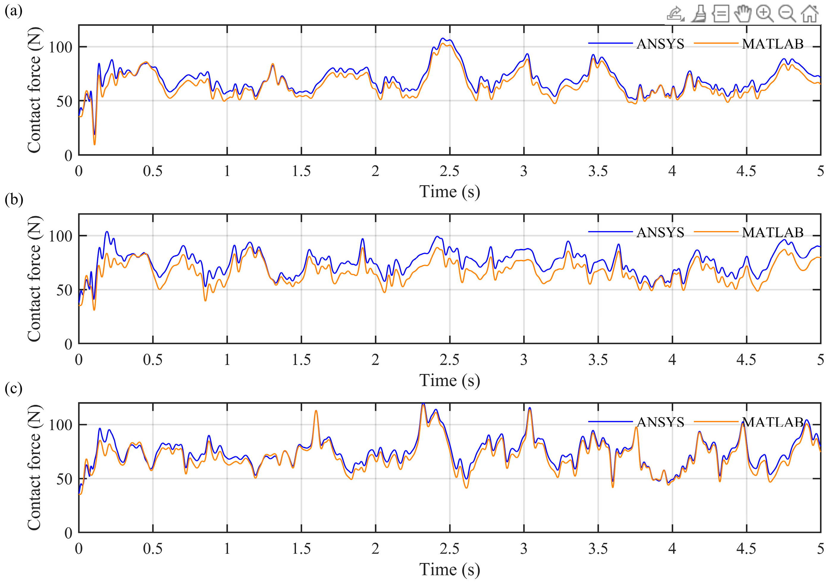
where the contact stiffness K is taken as 50,000 KN/m, and d denotes the vertical relative displacement between the pantograph head and contact wire. The proposed pantograph-catenary model has been validated in ref. [26], thus no further validation is repeated here. Considering the critical role of the pantograph-catenary model under crosswind conditions in evaluating controller performance, this paper verifies the reliability of the model by comparing it with results from the commercial software ANSYS 2021R1. The same pantograph-catenary system is modeled in ANSYS, and the wind data is also used as inputs. Since three speed levels are selected in this study, images corresponding to a speed of 200–300 km/h and a crosswind speed of 15 m/s are chosen for comparison. In the Figure 6, MATLAB denotes the MATLAB-generated results, while ANSYS represents the ANSYS-generated results. It can be observed from the figures that the trends in both MATLAB and ANSYS are generally consistent, where the maximum relative difference between these two results is no more than 4.5%. This demonstrates the reliability of the constructed model.

2.5. Initial Simulation Results

This study first analyzes the coupled pantograph-catenary dynamic response under crosswind conditions. By establishing dynamic models under different operating conditions and train speeds, the contact force response characteristics of the system under crosswind disturbance are obtained. The contact force time-history curves are obtained through Equation (20). During simulations, the train speed and crosswind velocity were set to four distinct levels to examine contact pressure variations under different operating conditions. Time-history curve of pantograph-catenary coupled contact force under different working conditions are shown in Figure 7. Simulation results of contact force are shown in

Table 3. Simulation results of contact force under four crosswind speed levels.

Speed		Max/N	Min/N	$\stackrel{\wedge }{\mathit{F}}$/N	$\mathit{\sigma }$/N
200 km/h	0 m/s	96.23	29.89	72.90	10.79
	10 m/s	111.86	27.72	69.41	12.87
	20 m/s	122.92	−3.27	56.98	26.02
	30 m/s	202.67	−6.37	32.86	38.52
250 km/h	0 m/s	106.87	35.33	74.89	10.69
	10 m/s	89.58	30.73	66.74	10.48
	20 m/s	136.23	−2.56	58.88	27.74
	30 m/s	207.39	−5.63	34.32	38.06
300 km/h	0 m/s	127.42	35.33	77.84	16.73
	10 m/s	138.51	18.39	73.37	17.49
	20 m/s	154.59	−5.27	60.79	33.09
	30 m/s	231.76	−8.78	38.51	42.17

Where Max is the maximum value, Min is the minimum value, $\stackrel{\wedge }{F}$ is the average value, $\sigma$ is the Standard deviation.

. When the contact force reaches zero or negative values, it indicates a pantograph-catenary contact loss. As clearly observed in Figure 7, without crosswind, no contact loss occurs throughout the operation. However, when the crosswind speed exceeds a certain threshold, significant separation phenomena are observed at multiple time points, with the contact force exhibiting substantial fluctuations or even dropping to zero. These results demonstrate that crosswinds significantly affect the stability of pantograph-catenary systems, leading to intensified contact force fluctuations and even separation states, which seriously threaten train operational safety. Therefore, it is essential to implement measures to enhance the anti-interference capability and operational stability of pantograph-catenary systems under crosswind disturbances.

3. Neural Network-Based PID Control Method

3.1. PID Control

The PID control algorithm consists of proportional, integral, and derivative components, making it one of the most widely used control methods in engineering due to its simplicity, flexibility, and convenience [29,30]. The fundamental principle of PID control involves calculating the error $e(k)$ between the system feedback $y(k)$ and the target value $r(k)$, and by adjusting the proportional $K_P$, integral $K_I$, and derivative coefficients $K_D$ to achieve comprehensive system control.

According to [30], the relationship between the error and the control force in PID control is given by Equation (22):

$$u(k)=K_{P}e(k)+K_I{\displaystyle {\int }_0^{t}e(k)\mathrm{d}t}+K_D{\displaystyle \frac{\mathrm{d}e(k)}{\mathrm{d}t}}$$

(22)

Discretizing the above equation yields both positional PID and incremental PID algorithms. These two algorithms differ in structure: the positional PID directly computes the current control output, while the incremental PID calculates the control increment $\Delta u(k)$. The mathematical expression for the positional PID algorithm is shown in Equation (23):

$$u(k)=K_{P}e(k)+K_I{T}_s{\displaystyle {\sum }_{i=0}e(i)}+{\displaystyle \frac{K_D}{T_s}}\left[e(k)-e(k-1)\right]$$

(23)

where $T_s$ represent the sampling period.

The mathematical formulation of the incremental PID algorithm is expressed as follows:

$$\begin{array}{l}\Delta u(k)=u(k)-u(k-1)=K_P\left[e(k)-e(k-1)\right]+K_{i}e(k)\\ +K_d\left[e(k)-2e(k-1)+e(k-2)\right]\end{array}$$

(24)

where $e(k-1)$ and $e(k-2)$ represent the error terms at the (k−1)-th and (k−2)-th sampling instants, respectively. $K_i=K_I{T}_s$ and $K_d={\displaystyle \frac{K_D}{T_s}}$.

Standard deviation is calculated using the formula:

$$\sigma =\sqrt{{\displaystyle \frac{{\displaystyle \sum {\left(x_i-\mu \right)}^2}}{N}}}$$

(25)

where $x_i$ is the value of each individual data point, $\mu$ is the population mean, N is the total number of data points in the population.

3.2. RBF-PID Control

Due to the limited regulatory effect of traditional PID control in nonlinear and time-varying systems, which makes it difficult to adapt to dynamic changes or complex working conditions, a radial basis function (RBF) neural network is incorporated into the control scheme for improvement [31]. This control strategy, which combines traditional PID control with an RBF neural network, represents an adaptive control method. This three-layer neural network exhibits exceptional approximation capabilities, making it particularly suitable for nonlinear, time-varying systems. It enables online adjustment of PID parameters to better accommodate pantograph–catenary contact force control requirements.

In the control strategy, the RBF neural network dynamically adjusts its center points c, widths b, and weights w based on input data, thereby modifying PID gains. The Jacobian information of the controlled object refers to the partial derivative of the output variables with respect to the control variables. In the algorithm, the adjusted PID parameters are obtained through gradient descent by utilizing this result, the existing PID parameters, the learning rate, and the PID input variables. This process ultimately achieves adaptive tuning of PID parameters. The control schematic diagram of RBF-PID is illustrated in Figure 8.

In Figure 8, r is the target value, e denotes the error signal, u represents the control force, y is the actual output, $y_m$ indicates the output layer value, and $\Delta k_p,\Delta k_i,\Delta k_d$ stands for the adjustment quantity.

The performance metrics of the neural network are defined as follows:

$$J={\displaystyle \frac{1}{2}}{\left(y(k)-y_m(k)\right)}^2$$

(26)

The tuning indices are as follows [21]:

$$E(k)={\displaystyle \frac{1}{2}}{e}^2(k)$$

(27)

In this system, Gaussian basis functions are typically employed as the nonlinear mapping functions. The Gaussian basis function is defined as [21]:

$$h_j=\exp \left({{\displaystyle \frac{-‖X-C_j‖}{2b_j^2}}}^2\right)\left(j=1,2,3,\dots ,m\right)$$

(28)

where $X=\left[x_1,x_2,x_3,\dots ,x_n\right]$ is the input vector of the network, and $C_j=\left[c_1,c_2,c_3,\dots ,c_n\right]$ represents the center vector of the network nodes. The output $y_m=wh$ is denoted as, and in the neural network, the output weight vector w, basis width vector b, and center node vector c are learned via the gradient descent method, formulated as:

$$\begin{array}{l}{w}_j(k)=w_j(k-1)+\alpha (y(k)-y_m(k))h_j+\beta (w_j(k-1)-w_j(k-2))\\ +\gamma (w_j(k-2)-w_j(k-3))\end{array}$$

(29)

$$\begin{array}{l}{b}_j(k)=b_j(k-1)+\alpha ((y(k)-y_m(k))w_j{h}_j{{\displaystyle \frac{‖X-C_j‖}{b_j^3}}}^2+\beta (b_j(k-1)-b_j(k-2))\\ +\gamma (b_j(k-2)-b_j(k-3))\end{array}$$

(30)

$$\begin{array}{l}{c}_{ji}(k)=c_{ji}(k-1)+\alpha ((y(k)-y_m(k))w_j{\displaystyle \frac{x_j-c_{ji}}{b_j^2}}+\beta (c_{ji}(k-1)-c_{ji}(k-2))\\ +\gamma (c_{ji}(k-2)-c_{ji}(k-3))\end{array}$$

(31)

where $\alpha$ denotes the learning rate, and $\beta ,\gamma$ represents the momentum factor. Typically, the center points c are primarily selected based on methods such as K-means [32], the widths b are mainly chosen using fixed-width methods, and the weights w are initially randomized. In this study, these parameters are empirically determined.

The adjustment of PID parameters is given by:

$$\left\{\begin{array}{c}\Delta K_{\mathrm{p}}=\alpha e(k){\displaystyle \frac{\mathrm{\delta }y(k)}{\mathrm{\delta }\Delta u}}(e(k)-e(k-1))\\ \Delta K_i=\alpha e(k){\displaystyle \frac{\mathrm{\delta }y(k)}{\mathrm{\delta }\Delta u}}e(k)\\ \Delta K_d=\alpha e(k){\displaystyle \frac{\mathrm{\delta }y(k)}{\mathrm{\delta }\Delta u}}(e(k)-2e(k-1)+e(k-2))\end{array}\right.$$

(32)

where ${\displaystyle \frac{\mathrm{\delta }y(k)}{\mathrm{\delta }\Delta u}}={\displaystyle {\sum }_{j=1}^m{w}_j{h}_j}{\displaystyle \frac{c_j-x_1}{2b_j^2}}$ represents the Jacobian information of the controlled plant [20], which is identified through the neural network. In the controller, the control output $u(k)=u(k-1)+\Delta u(k)$ is obtained based on the parameter adjustments.

3.3. RBF-PID Control Method of the Present Pantograph-Catenary System

The designed controller is applied to regulate the pantograph head in this study, where the contact force is adjusted by applying control forces to the pantograph. For practical implementation, electromagnetic actuators could be employed as the actuating deices due to their suitability for installation on the pantograph head, low power requirements, minimal mass addition, wide bandwidth, and reduced sensitivity to high-voltage environments [33]. Although such actuators have not yet been fully deployed in operational systems, their gradual refinement in future developments is expected to enable practical applications. The contact force is derived from the pantograph head acceleration and the pantograph head suspension force, which is consistent with actual engineering practices.

The neural network structure of the RBF-PID controller in this study adopts a 3-6-1 architecture (with 3 nodes in the input layer, 6 nodes in the hidden layer, and 1 node in the output layer), where $\left[\begin{array}{ccc}\Delta u(k)& y(k)& y(k-1)\end{array}\right]$ is the controller input vector. The initial values of the center points c, widths b, and weights w are set to 20, 10, and 5, respectively. The output of the output layer is computed through forward propagation, while the center points, widths, and weights are updated via backpropagation. The Jacobian information is utilized to compute the incremental changes in PID parameters, which are then applied in the controller to ultimately determine the final control output. To evaluate the performance of the improved control strategy in the pantograph-catenary coupling model, experiments are conducted under three different operating speeds and three different crosswind speeds for analysis and verification. Figure 9 illustrates the neural network structure.

This study adopts an offline-online integrated neural network PID strategy. This approach reduces training time and enhances computational speed compared to purely online methods. Specifically, 5 s of data are collected from the pantograph-catenary system, followed by 50 iterative cycles to derive the control command required every 0.1 s. The resulting 50 sets of control outputs are applied to the system to obtain the contact force, and the cycle repeats to optimize the control performance. In practical computations, this method significantly reduces the computational burden: the offline training process for the 5 s operational data requires approximately 150 min, which can be executed on a standard computer, while the online training phase only takes 10 milliseconds. Additionally, the sensors used operate at a sampling frequency of 10,000 Hz, ensuring real-time responsiveness.

The proposed control strategy is implemented as follows: the training target is the contact force sampled every 0.1 s, aiming to achieve accurate tracking of the desired reference values. Special emphasis is placed on control optimization when the contact force falls below 50 N (indicating contact loss). The RBF-PID control strategy can be implemented through the procedure in

Table 4. Pseudocode of the controller.

Controller Output Process
1. Start
2. For each time step k = 1 to n
Calculate contact force of controlled object
For each iteration i = 1 to 50
Compute hidden layer output h using Equation (28)
Update c, b, w using Equations (29)–(31)
Calculate parameter adjustment using Equation (32)
Compute control output using updated parameters and Equation (24)
Output $u(i)$
End inner loop
End outer loop
3. End

.

4. Results and Discussion

4.1. Control Results

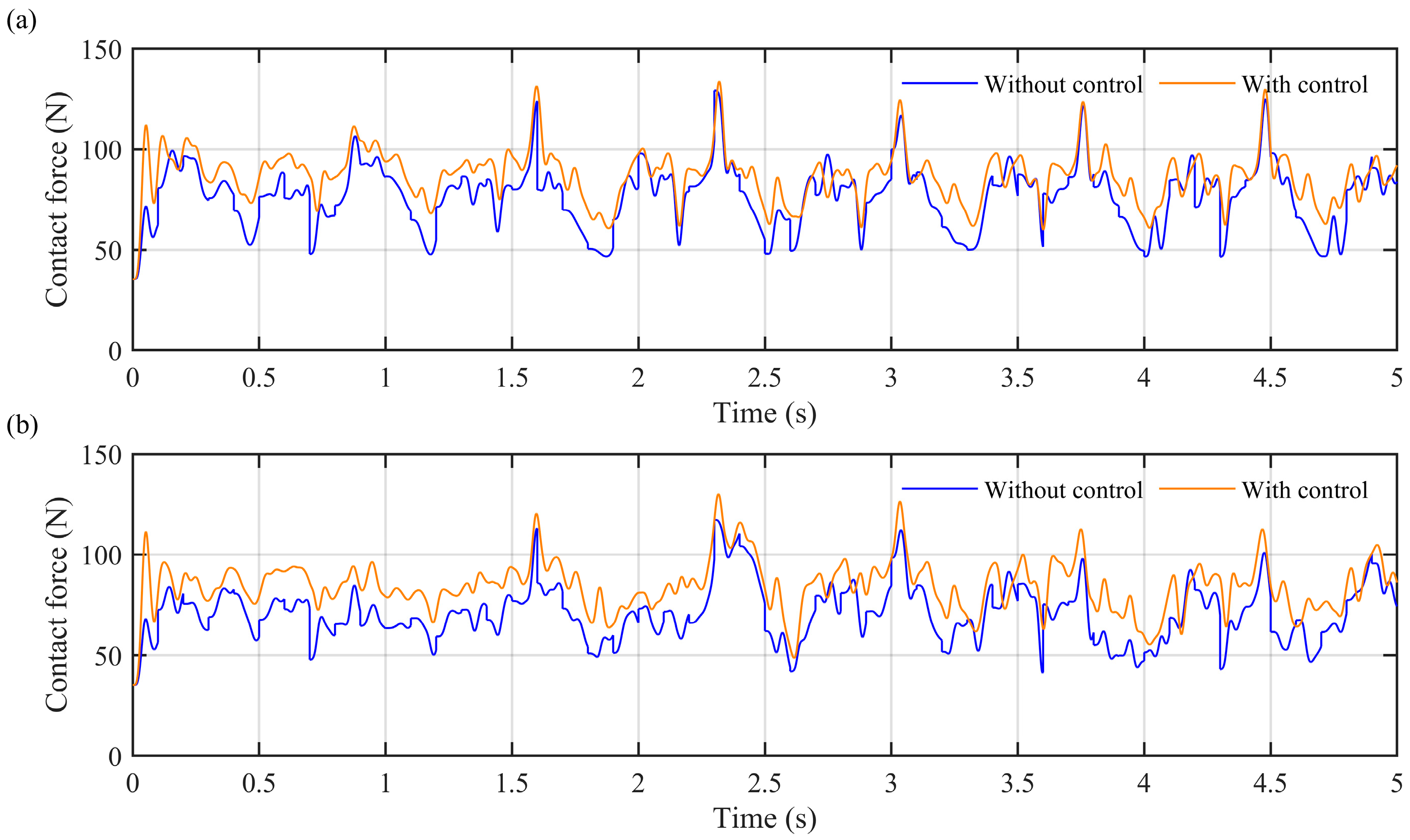
Based on the aforementioned model, this study investigates control strategies for the pantograph-catenary coupled system under crosswind conditions of 5–25 m/s and operating speeds of 200–300 km/h. The initial control implementation focuses on the pantograph under varying wind speeds of 5–25 m/s at an operating speed of 200 km/h. It should be noted that uncontrolled models may exhibit slight variations in simulations due to the adoption of different control strategies. For comparative purposes, this paper selects the uncontrolled model under PID control as the benchmark case. In the figures, Without control refers to the curve without applied control force, while With control indicates the curve under RBF-PID control. The percentage values represent the reduction rate of the standard deviation of the system after control implementation compared to the uncontrolled case.

The control outcomes are presented Figure 10 as follows:

Table 5. Comparison of standard deviations for different control strategies under varying crosswind conditions at 200 km/h.

Wind Speed/(m/s)	$\mathit{\sigma }$/N
	Without Control	PID Control	RBF-PID Control
5 m/s	10.19	9.76 (4.22%)	8.94 (12.27%)
15 m/s	11.72	11.67 (0.43%)	8.78 (25.09%)
25 m/s	13.35	12.96 (2.92%)	10.10 (24.34%)

results indicate that compared with conventional control methods, the proposed approach can more effectively reduce vibration amplitudes at a speed of 200 km/h under various crosswind conditions, thereby significantly improving system operational stability. Furthermore, this method successfully eliminates the contact loss phenomenon occurring around 3.8 s and reduces the overall contact loss rate to zero, exhibiting excellent crosswind resistance control performance.

Table 6. Controller parameter at 200 km/h.

Parameter	PID			RBF-PID
	5 m/s	15 m/s	25 m/s	5 m/s	15 m/s	25 m/s
P	0.3	1	0.01	0.3	1	0.3
I	0.00001	0.00001	0.0001	0.00001	0.00001	0.0001
D	0.1	0.1	1	0.1	0.1	0.5

present the tuned parameters.

The control performance at 250 km/h under 5–25 m/s crosswinds is presented Figure 11 below:

The comparative results in

Table 7. Comparison of standard deviations for different control strategies under varying crosswind conditions at 250 km/h.

Wind Speed/(m/s)	$\mathit{\sigma }$/N
	Without Control	PID Control	RBF-PID Control
5 m/s	10.25	10.04 (2.05%)	8.10 (20.98%)
15 m/s	10.22	10.04 (1.76%)	9.26 (9.39%)
25 m/s	27.43	24.21 (11.74%)	17.19 (37.33%)

indicate that the improved control method shows significant effectiveness under crosswinds of 5–25 m/s at 250 km/h, enabling the contact force to better approach the target value with markedly reduced fluctuations. Most notably, the method completely eliminates contact loss (0% contact loss rate), displaying outstanding resistance to crosswind disturbances.

Table 8. Controller parameter at 250 km/h.

Parameter	PID			RBF-PID
	5 m/s	15 m/s	25 m/s	5 m/s	15 m/s	25 m/s
P	0.01	0.01	0.0001	0.01	0.01	0.7
I	0.00001	0.00001	0.0000007	0.00001	0.00001	0.0001
D	0.1	0.1	0.7	0.1	0.1	0.1

present the tuned parameters.

The control performance at 300 km/h under 5–15 m/s crosswinds is presented Figure 12 below:

The comparative results in

Table 9. Comparison of standard deviations for different control strategies under varying crosswind conditions at 300 km/h.

Wind Speed/(m/s)	$\mathit{\sigma }$/N
	Without Control	PID Control	RBF-PID Control
5 m/s	15.68	15.68 (0%)	12.81 (18.30%)
15 m/s	13.9	13.89 (0.14%)	12.69 (8.71%)

indicate that the improved control method can more effectively maintain the contact force close to the target value while significantly reducing its standard deviation under crosswinds of 5–15 m/s at 300 km/h, demonstrating superior anti-crosswind control performance. As can be seen from the data in Table 9, under the conditions of a 5 m/s wind speed and a train speed of 300 km/h, the PID control fails while the RBF-PID control remains effective, which demonstrates the validity of the RBF-PID control strategy. The adaptive ranges of the parameters $K_P$, $K_i$ and $K_d$ are 0.0001–1.55, 0.000001–0.02, and 0.01–0.16, respectively.

Table 10. Controller parameter at 300 km/h.

Parameter	PID		RBF-PID
	5 m/s	15 m/s	5 m/s	15 m/s
P	0	0.0001	0.0001	0.0001
I	0	0.000001	0.00001	0.000001
D	0	0.0001	0.01	0.01

present the tuned parameters.

However, operation at 300 km/h under 25 m/s wind speeds was not considered in this study due to the excessive wind velocity that could potentially cause train service suspension.

4.2. Robustness Analysis of the Control System

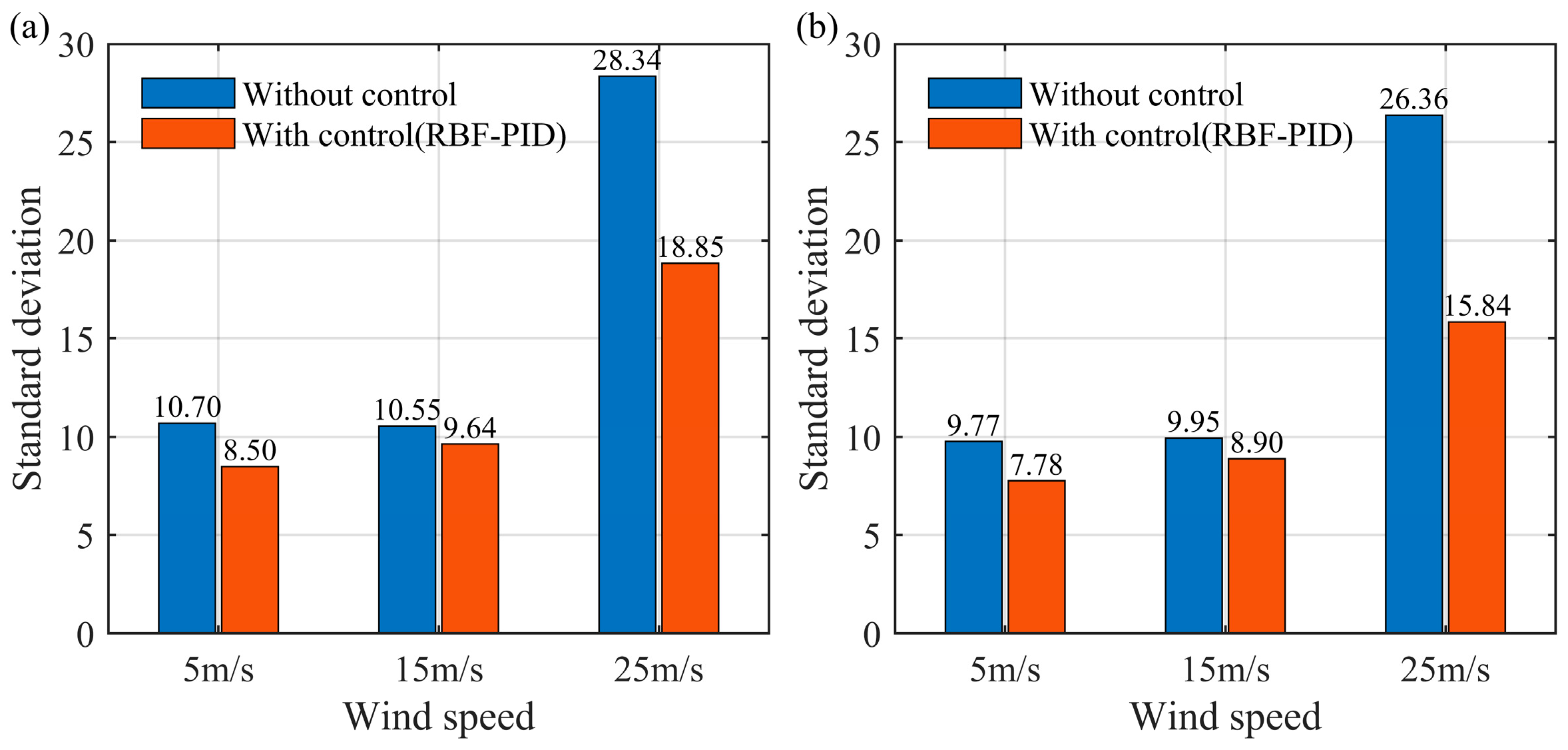
In practical applications, model parameters may become uncertain due to factors such as aging. Therefore, this study simulates such variations by altering pantograph parameters and evaluates the controller’s capability to handle model parameter uncertainties [32]. Fluctuations in pantograph parameters may lead to variations in contact force, thereby degrading the original system performance and significantly affecting the contact quality. To assess the robustness of the proposed controller, its performance was evaluated under parameter perturbation conditions. Specifically, random parameter fluctuations were simulated by altering the pantograph suspension stiffness by $\pm$10%, with the corresponding control performance results illustrated in Figure 13. As observed in the figure, the proposed control method effectively suppresses fluctuations even under parameter variations, demonstrating its strong robustness.

5. Conclusions

This study presents a neural network PID-based active control strategy for pantograph-catenary systems operating under crosswind conditions, effectively overcoming the inadequate performance of traditional PID controllers in complex, time-varying environments. A pantograph-catenary interaction model under crosswind was established using a truncated beam approach within the MATLAB simulation environment, incorporating crosswind effects modeled via wind spectra. A nonlinear neural network PID controller was designed and integrated into this dynamic system. The results indicate that the RBF-PID controller effectively enhances the dynamic response characteristics of the pantograph-catenary system, significantly suppresses contact force fluctuations, and nearly eliminates the offline phenomenon under crosswind disturbances. Compared with conventional PID controllers, the neural network PID approach ensures more stable and reliable current collection. Robustness analyses further demonstrate that the controller consistently maintains high performance despite variations in pantograph parameters, indicating strong adaptability to practical engineering applications. For real-world implementation, it is feasible to embed micro-actuators within the pantograph head to enable real-time control adjustment, thereby improving adaptability to changing catenary conditions and enhancing current collection stability. While certain engineering challenges-such as high-voltage insulation, spatial constraints, and equipment reliability-remain to be addressed, ongoing advances in materials science, micro-actuation, and embedded control technology are accelerating progress toward practical deployment of active pantograph control. Overall, the method proposed in this study not only provides a solid theoretical foundation and technical guidance for improving the stability of pantograph-catenary systems under wind conditions, but also offers novel insights and references for the intelligent and adaptive control of high-speed rail systems under complex external disturbances.

References

1. Song, Y.; Liu, Z.; Wang, H.; Lu, X.; Zhang, J. Nonlinear analysis of wind-induced vibration of high-speed railway catenary and its influence on pantograph–catenary interaction. Veh. Syst. Dyn. 2016, 54, 723–747. [Google Scholar] [CrossRef]
2. Song, Y.; Duan, F.; Gao, S.; Wu, F.; Liu, Z. Crosswind effects on current collection quality of railway pantograph–catenary: A case study in Chengdu–Chongqing passenger special line. IEEE Trans. Instrum. Meas. 2021, 71, 1–13. [Google Scholar] [CrossRef]
3. Song, Y.; Zhang, M.; Øiseth, O.; Rønnquist, A. Wind deflection analysis of railway catenary under crosswind based on nonlinear finite element model and wind tunnel test. Mech. Mach. Theory 2022, 168, 104608. [Google Scholar] [CrossRef]
4. Song, Y.; Zhang, M.; Wang, H. A response spectrum analysis of wind deflection in railway overhead contact lines using pseudo-excitation method. IEEE Trans. Veh. Technol. 2021, 70, 1169–1178. [Google Scholar] [CrossRef]
5. Luo, Q.; Mei, G.; Chen, G.; Zhang, W. Study of pantograph-catenary system dynamic in crosswind environments. Veh. Syst. Dyn. 2024, 62, 813–836. [Google Scholar] [CrossRef]
6. Niu, J.-Q.; Zhou, D. Aerodynamic effects of ravine wind to pantograph of high-speed train arriving and leaving a tunnel. In Proceedings of the CICTP 2014: Safe, Smart, and Sustainable Multimodal Transportation Systems, Changsha, China, 4–7 July 2014; pp. 162–175. [Google Scholar] [CrossRef]
7. Daocharoenporn, S.; Mongkolwongrojn, M. Effects of crosswind on pantograph–catenary wear using nonlinear multibody system dynamic algorithms. World Electr. Veh. J. 2023, 14, 250. [Google Scholar] [CrossRef]
8. Li, Y.-H.; Cao, Y.; Wu, Y.-X.; Bai, X.-N.; Mao, J.-W. Pantograph-catenary contact reliability analysis under crosswind. Int. J. Struct. Integr. 2021, 12, 629–644. [Google Scholar] [CrossRef]
9. Xie, Q.; Zhi, X. Wind tunnel test of an aeroelastic model of a catenary system for a high-speed railway in China. J. Wind Eng. Ind. Aerodyn. 2019, 184, 23–33. [Google Scholar] [CrossRef]
10. Pan, L.; Yang, C.; Shen, X.; He, F.; Zhu, X.; Zhao, Y.; Yuan, Y.; Zhao, Q.; Meng, Q.; Dong, B. Fatigue analysis of railway catenary dropper based on its stress incorporating displacement loading and fluctuating wind load. Sci. Prog. 2025, 108, 00368504241311432. [Google Scholar] [CrossRef] [PubMed]
11. Duan, F.; Song, Y.; Gao, S.; Liu, Y.; Chu, W.; Lu, X.; Liu, Z. Study on aerodynamic instability and galloping response of rail overhead contact line based on wind tunnel tests. IEEE Trans. Veh. Technol. 2023, 72, 7211–7220. [Google Scholar] [CrossRef]
12. Chen, X.; Zhang, X.; Wang, Y.; Wang, X.; Zhong, D. Influence of environmental wind on fluctuation velocity of contact wire of high-speed railway. J. Traffic Transp. Eng. 2020, 20, 93. [Google Scholar] [CrossRef]
13. Song, Y.; Ouyang, H.; Liu, Z.; Mei, G.; Wang, H.; Lu, X. Active control of contact force for high-speed railway pantograph-catenary based on multi-body pantograph model. Mech. Mach. Theory 2017, 115, 35–59. [Google Scholar] [CrossRef]
14. Song, Y.; Liu, Z.; Ouyang, H.; Wang, H.; Lu, X. Sliding Mode Control with PD Sliding Surface for High-Speed Railway Pantograph-Catenary Contact Force under Strong Stochastic Wind Field. Shock Vib. 2017, 2017, 4895321. [Google Scholar] [CrossRef]
15. Ren, Z.; Wang, Y.; Mu, X.; Chen, X.; Chang, Z. Active Control of Pantograph Sliding Mode Under Fluctuating Wind Excitation. In Proceedings of the International Conference on Electrical and Information Technologies for Rail Transportation, Beijing, China, 19–21 October 2023; pp. 215–222. [Google Scholar] [CrossRef]
16. Zhang, J.; Huang, F.; Liu, T.; Xu, A.; Li, Y.; Ji, P.; Liu, T. An external design on performance improvement of the transition windbreak wall between an embankment and a hill cut along the high-speed railway. Transp. Saf. Environ. 2025, 7, tdaf010. [Google Scholar] [CrossRef]
17. Dong, X.; Liu, T.; Shi, Z.; Xia, Y.; Yang, F.; Chen, Z. Influence of porosity of reformed earth embankment windbreak wall on flow field and displacement of catenary under crosswinds. J. Wind Eng. Ind. Aerodyn. 2021, 214, 104652. [Google Scholar] [CrossRef]
18. Yang, G. State filtered disturbance rejection control. Nonlinear Dyn. 2025, 113, 6739–6755. [Google Scholar] [CrossRef]
19. Yang, G.; Yao, J. Multilayer neurocontrol of high-order uncertain nonlinear systems with active disturbance rejection. Int. J. Robust Nonlinear Control 2024, 34, 2972–2987. [Google Scholar] [CrossRef]
20. Qiu, R. Adaptive Control of Vehicle Active Suspension Based on Neural Network Optimization. In Proceedings of the 2021 7th International Conference on Energy Materials and Environment Engineering (ICEMEE 2021), Zhangjiajie, China, 23–25 April 2021; p. 03046. [Google Scholar] [CrossRef]
21. Zhao, W.; Gu, L. RBF neural network-based adaptive PID controller for active suspension. Authorea Prepr. 2023. [Google Scholar] [CrossRef]
22. Duan, J.; Zhao, H.; Zhou, C.; Peng, Z.; Chen, X. Research on control strategy of active suspension based on improved RBF neural network. In Proceedings of the International Workshop on Automation, Control, and Communication Engineering (IWACCE 2024), Hohhot, China, 19–21 August 2024; pp. 502–508. [Google Scholar] [CrossRef]
23. Liu, J.; Li, X.; Zhang, X.; Chen, X. Modeling and Simulation of Energy-Regenerative Active Suspension Based on BP Neural Network PID Control. Shock Vib. 2019, 2019, 4609754. [Google Scholar] [CrossRef]
24. Effendi, M.; Pande, D.; Harnany, D.; Hendrowati, W. Optimization of PID Control Parameters for Quarter-Vehicle Model Active Suspension System Using Back Propagation Neural Network and Genetic Algorithm Methods. In Proceedings of the International Conference on Mechanical Engineering, Dhaka, Bangladesh, 18–19 December 2023; pp. 147–154. [Google Scholar] [CrossRef]
25. Liu, Z.; Jönsson, P.-A.; Stichel, S.; Rønnquist, A. Implications of the operation of multiple pantographs on the soft catenary systems in Sweden. Proc. Inst. Mech. Eng. Part F J. Rail Rapid Transit. 2016, 230, 971–983. [Google Scholar] [CrossRef]
26. Xu, Y.; Liu, Z.; Stichel, S.; Zhu, W.; Lei, J.; Yao, Y. A comparative study on the influence of typical track failures on high-speed pantograph-catenary interaction dynamics. Veh. Syst. Dyn. 2024, 62, 2883–2911. [Google Scholar] [CrossRef]
27. Davenport, A.G. The application of statistical concepts to the wind loading of structures. Proc. Inst. Civ. Eng. 1961, 19, 449–472. [Google Scholar] [CrossRef]
28. Wang, B.H.; Wang, D.B.; Ali, Z.A.; Ting Ting, B.; Wang, H. An overview of various kinds of wind effects on unmanned aerial vehicle. Meas. Control 2019, 52, 731–739. [Google Scholar] [CrossRef]
29. Borase, R.P.; Maghade, D.; Sondkar, S.; Pawar, S. A review of PID control, tuning methods and applications. Int. J. Dyn. Control 2021, 9, 818–827. [Google Scholar] [CrossRef]
30. Patil, R.S.; Jadhav, S.P.; Patil, M.D. Review of intelligent and nature-inspired algorithms-based methods for tuning PID controllers in industrial applications. J. Robot. Control 2024, 5, 336–358. [Google Scholar] [CrossRef]
31. Mohammadzaheri, M.; Chen, L.; Grainger, S. A critical review of the most popular types of neuro control. Asian J. Control 2012, 14, 1–11. [Google Scholar] [CrossRef]
32. Ma, D.; Song, M.; Yu, P.; Li, J. Research of RBF-PID control in maglev system. Symmetry 2020, 12, 1780. [Google Scholar] [CrossRef]
33. Ferré, F.G.; Johansson, A.; Herrmann, L.; Korbel, J.; Erford, T.; Riechert, U. A lightweight electromagnetic actuator for high voltage DC power grids. Addit. Manuf. 2019, 27, 533–539. [Google Scholar] [CrossRef]
Figure 1. Coupled pantograph-catenary system under crosswind conditions.
Machines 13 00897 g001
Figure 2. Catenary model.
Machines 13 00897 g002
Figure 3. Two-mass pantograph model.
Machines 13 00897 g003
Figure 4. Catenary model under crosswind excitation.
Machines 13 00897 g004
Figure 5. Stochastic wind speed spectra and corresponding time-history curves under different wind speed levels: (a) Davenport wind speed spectrum at 5 m/s; (b) Davenport wind speed spectrum at 15 m/s; (c) Davenport wind speed spectrum at 25 m/s; (d) Time-history curve of stochastic wind speed at 5 m/s; (e) Time-history curve of stochastic wind speed at 5 m/s; (f) Time-history curve of stochastic wind speed at 5 m/s.
Machines 13 00897 g005
Figure 6. Comparison of MATLAB and ANSYS Verification Results: (a) 200 km/h, 15 m/s; (b) 250 km/h, 15 m/s; (c) 300 km/h, 15 m/s.
Machines 13 00897 g006
Figure 7. Time-history curve of pantograph-catenary coupled contact force: (a) 200 km/h, 0–30 m/s; (b) 250 km/h, 0–30 m/s; (c) 300 km/h, 0–30 m/s.
Machines 13 00897 g007
Figure 8. Schematic of RBF-PID control.
Machines 13 00897 g008
Figure 9. An RBF neural network with a three-layer structure.
Machines 13 00897 g009
Figure 10. Control results under different crosswind conditions at a speed of 200 km/h: (a) V = 200 km/h, U = 5 m/s; (b) V = 200 km/h, U = 15 m/s; (c) V = 200 km/h, U = 25 m/s.
Machines 13 00897 g010
Figure 11. Control results under different crosswind conditions at a speed of 250 km/h: (a) V = 200 km/h, U = 5 m/s; (b) V = 200 km/h, U = 15 m/s; (c) V = 200 km/h, U = 25 m/s.
Machines 13 00897 g011
Figure 12. Control results under different crosswind conditions at a speed of 300 km/h: (a) V = 200 km/h, U = 5 m/s; (b) V = 200 km/h, U = 15 m/s.
Machines 13 00897 g012
Figure 13. Robustness analysis results under pantograph suspension stiffness variations at 250 km/h: (a) Parameter increase; (b) Parameter decrease.
Machines 13 00897 g013