A Multi-Category Defect Detection Model for Rail Fastener Based on Optimized YOLOv8n

Abstract

Currently, object detection-based rail fastener defect detection methods still face challenges such as limited detection categories, insufficient accuracy, and high computational complexity. To this end, the YOLOv8n-FDD, an advanced multi-category fastener defect detection model designed upon the YOLOv8n with comprehensive optimizations is developed in this paper. Concretely, by introducing the CUT-based style transfer model to generate diverse defect samples, the concern due to imbalanced distribution of sample categories is effectively alleviated. The CA mechanism is incorporated to enhance the feature extraction capability, and the bounding box loss function is further upgraded to improve the model’s generalization performance. With respect to efficiency, the Conv and c2f modules of the YOLOv8n model are, respectively, replaced with the GSConv and VoVGSPCP modules, accordingly achieving a lightweight design. Comparative experimental results demonstrate that the presented YOLOv8n-FDD model outperforms several classic object detection models in terms of detection accuracy, detection speed, model size, and computational complexity.

1. Introduction

The rail fastening system (hereinafter referred to as ‘fastener’), as a vital part of the track structure, serves to connect the rail and the underlying supporting structure. It performs functions such as fixing the rail position and providing elastic support to the rail, thus playing a crucial role in ensuring the stability and smoothness of the track structure as well as the safe operation of trains [1,2,3].

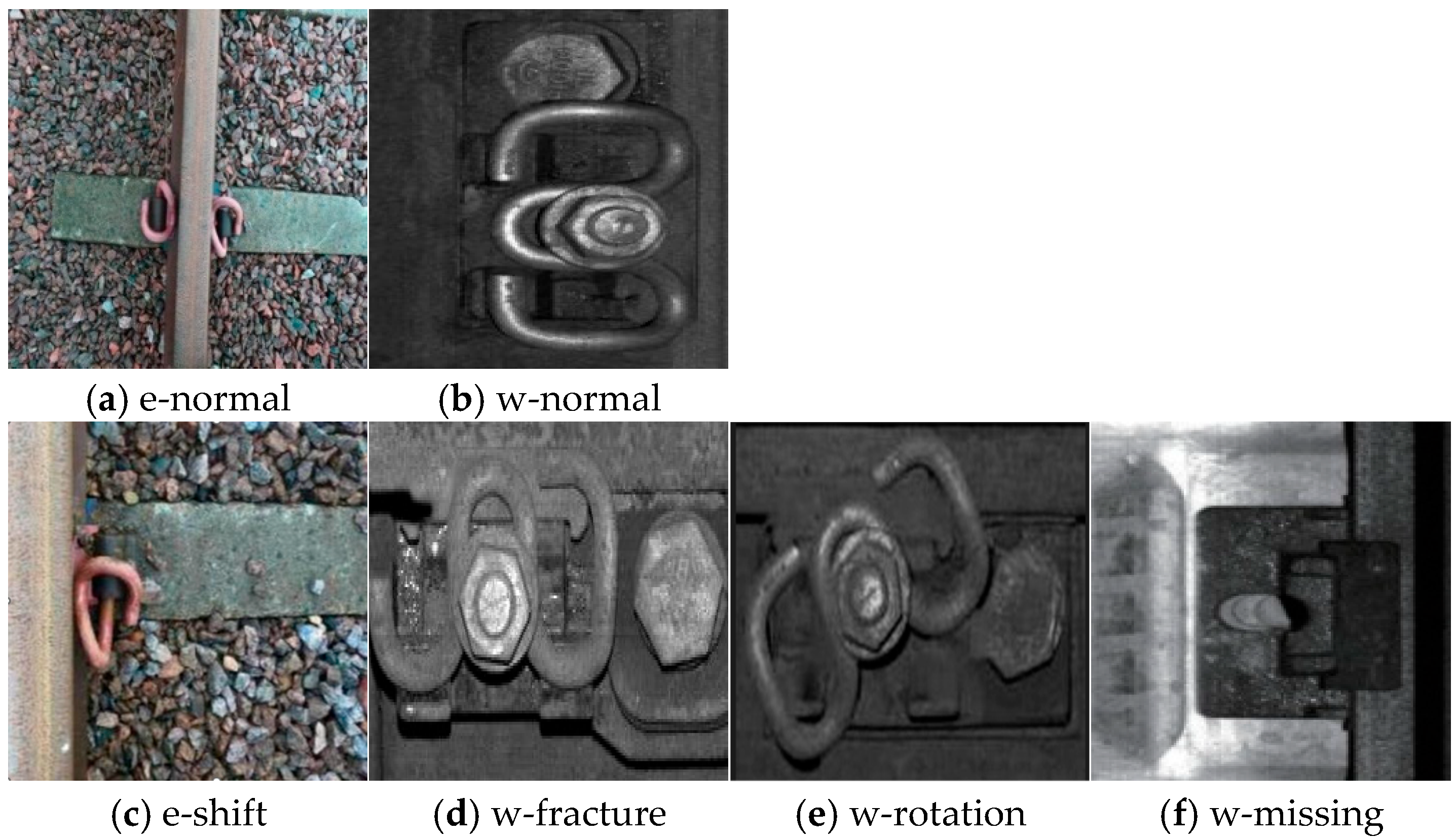
The fastener is primarily composed of three categories of components: the spring clip, the bolt, and the rail pad, and its functions are achieved through the coordination among these individual parts, as depicted in Figure 1. Under the long-term combined effects of cyclic train dynamic loads and complex and variable environmental loads, some typical damage and degradation issues have been exposed in fasteners currently in operation, e.g., fracture, missing and rotation of spring clips [4,5], protrusion and breakage of bolts [6,7], as well as aging and crushing of rail pads [8], etc. Such issues will lead to the attenuation or loss of fastening pressure and elastic support performance, thereby reducing the integrity and stability of the track structure, causing local damage or even overall failure of the track structure, ultimately deteriorating ride quality and endangering running safety. Therefore, the detection of the service condition of fasteners has always been a research focus.

Traditional fastener defect detection methods heavily rely on manual periodic inspections and empirical judgments, resulting in temporal discontinuity, spatial gaps, and lack of rigor in diagnosis. In recent years, with the rapid development of computer technology, intelligent detection of fastener defects has become a current research hotspot. Wang et al. [9] transformed the original image into HOG feature vectors and subsequently generated left–right and up–down symmetrical images, respectively, and finally achieved the detection of defective fasteners. The detection of missing fasteners was conducted through combining the stability of the fastener edge contours and template matching with curve feature projection [10]. Hu et al. [11] identified and located loose fasteners by utilizing a temporal Bayesian approach in conjunction with track vibration data. Fan et al. [12] proposed an image recognition method optimized by an IFOA algorithm on the basis of an improved SVM model, which was subsequently applied to the abnormal monitoring of fasteners. Considerable progress has been made in the research of fastener defect detection using the aforementioned methods. Nevertheless, several pressing issues remain to be addressed. For instance, the recognition of numerous edge feature points on some fasteners results in a complex sorting and iteration process. Secondly, Bayesian algorithms can be sensitive to outliers and noise when processing vibration data, and the presence of significant interference or abnormalities in the data can lead to the accumulation of errors, thereby affecting the detection accuracy. Additionally, due to the diversity of shapes and backgrounds, it is challenging to manually design accurate and robust features for fastener components using SVM models, consequently hindering the improvement of detection precision.

Nowadays, research on fastener defect detection based on deep learning technologies has emerged continuously, with object detection methods serving as the primary representative. One type of method is based on the end-to-end one-stage algorithm, primarily represented by the YOLO series of models [13]. For example, Hsieh et al. [14] implemented the detection of missing and fracture of spring clips by applying the YOLOv4Tiny model. Li et al. [15] proposed a novel method for detecting fastener defects by introducing the CBAM attention mechanism and a weighted bidirectional feature pyramid network on the basis of the YOLOv5s model. Meanwhile, Cai et al. [16] presented the FSS-YOLO detection model by improving the YOLOv5n model, which combines the morphological characteristics of fastener bolts to achieve rapid detection of bolt defects. The aforementioned methods have demonstrated remarkable advantages in fastener defect detection owing to their fast detection speed and ease of implementation and deployment. However, due to the fact that these methods generally require only one forward propagation to complete detection, there may be certain limitations in terms of localization accuracy, particularly when dealing with clustered targets, where their performance still needs further enhancement and optimization.

Another type of method involves the two-stage algorithm based on target candidate regions [17], which exhibits good robustness and high accuracy in complex scenarios. For instance, Bai et al. [18] proposed an optimized detection method based on an improved Faster R-CNN model, achieving effective localization of fastener defects. Moreover, Shang et al. [19] shifted the focus from qualitative analysis of fasteners to more accurate quantitative analysis by introducing an advanced image segmentation network model, namely Mask-FRCN. Nevertheless, it is noteworthy that due to the pixel-level segmentation processing involved in such two-stage algorithms, their computational complexity is relatively high, which to some extent limits the application in scenarios requiring high real-time object detection.

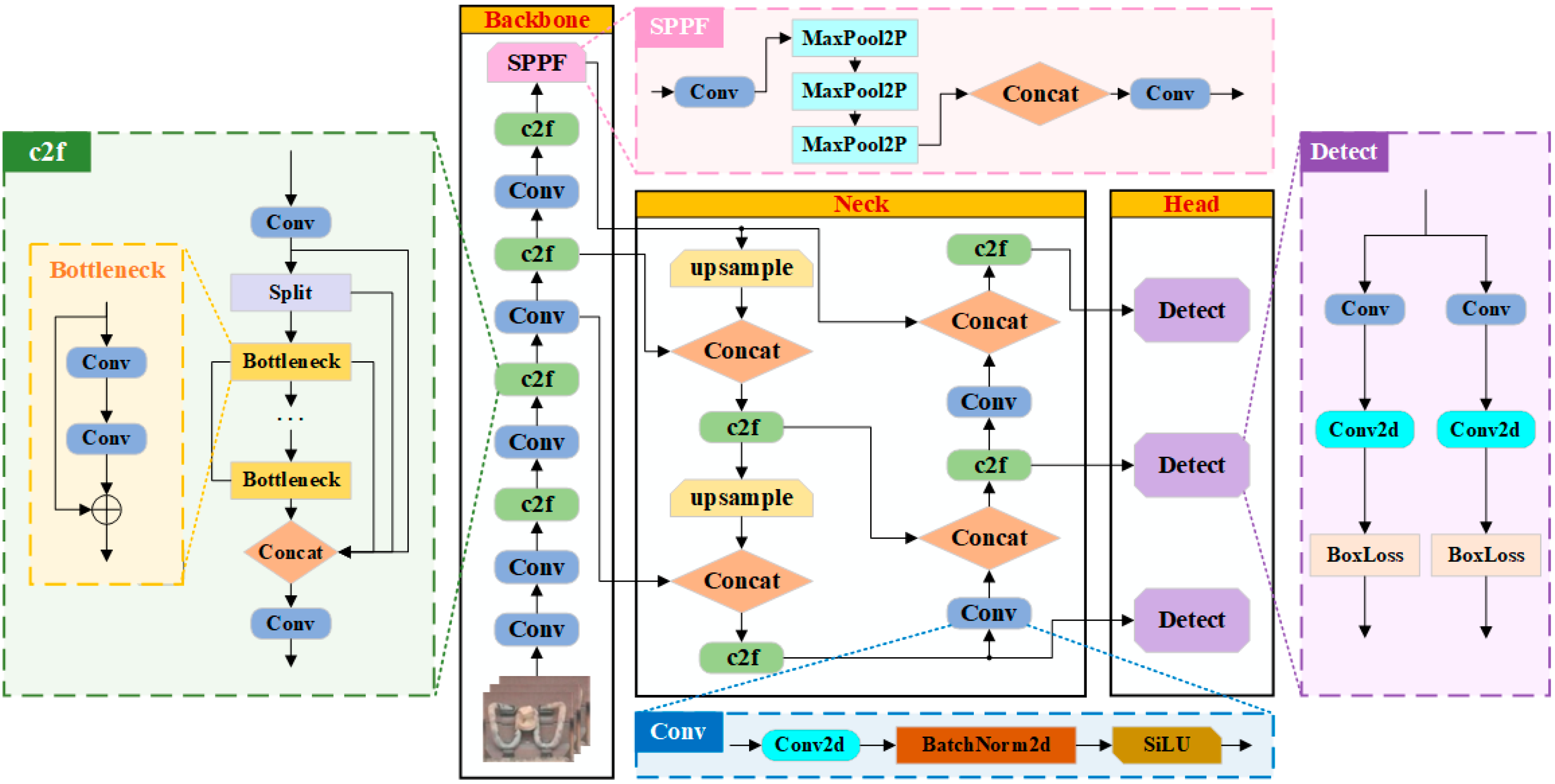
The YOLO series models have developed rapidly in the field of object detection [20,21]. Notably, the YOLOv8 [22] model stands out as the primary representative of the current YOLO series due to its advanced training methodology, high training efficiency, and robust generalization capability. To address the object detection tasks in complex and diverse real-world scenarios, the YOLOv8 model has been devised with multiple size variants, spanning various scales including n, s, m, l, and x, catering to a wide range of requirements from lightweight to high-performance. Among them, the YOLOv8n model, with its relatively compact size, boasts not only high detection accuracy but also the fastest detection speed, making it particularly suitable for tasks that demand extreme real-time performance. In light of this, this study focuses on the real-time detection of fastener defects, and an improved model namely YOLOv8n-Fastener Defect Detection (YOLOv8n-FDD) is developed, which is derived from and tailored based on the original YOLOv8n model, aiming to achieve high-precision and efficient detection of multiple common types of fastener defects.

2. Models and Improvements

2.1. Original YOLOv8n Model

The original YOLOv8n model comprises three parts: the backbone structure, the neck structure, and the head structure, with its overall architecture illustrated in Figure 2. The backbone structure is responsible for capturing and extracting rich feature information from input images, consisting of Convolutional (Conv) blocks, CSP Bottleneck with 2 convolutions (c2f) modules [23], and Spatial Pyramid Pooling Fast (SPPF) modules [24]. The neck structure, serving as a crucial connection between the backbone and the head structures, holds the pivotal task of further fusing and enhancing features. Ultimately, the fully fused features from the neck structure are transmitted to the head structure for final object detection at multiple scales.

2.2. Improvement of the YOLOv8n Model: YOLOv8n-FDD Model

The YOLOv8n model has demonstrated superior performance in detecting large objects on the general dataset COCO [25]. However, when dealing with image detection tasks of fasteners with complex backgrounds, its feature extraction and representation capabilities are still required to be optimized, and the model’s complexity also needs to be further reduced to enhance detection efficiency. Hence, this paper focuses on the specific requirements of the fastener defect detection, and targeted improvements are implemented to the YOLOv8n model, leading to the proposal of the YOLOv8n-FDD model. The detailed improvement strategies are elaborated as follows.

Firstly, in order to enhance the sensitivity of the model to subtle features of fastener images and its recognition ability under complex background interferences, the Coordinate Attention (CA) mechanism [26] is embedded between the c2f module and the SPPF module in the backbone structure, which enables the model to more effectively concentrate on key feature information of fastener images, thereby improving detection accuracy. Secondly, to reduce the computational cost while ensuring detection accuracy, the fourth traditional Conv block in the bottom-up direction of the backbone structure is replaced with a more efficient GSConv module [27], and the c2f module in the neck structure is upgraded to a VoVGSPCP module [27]. Lastly, to address potential issues of sample imbalance in the dataset and the subsequent decline in convergence during model training, the bounding loss function in the YOLOv8n model is optimized from Complete Intersection over Union (CIoU) [28] to Wise-IoU (WIoU) [29], thereby further enhancing the model’s training effectiveness and detection performance. The structure of the improved YOLOv8n-FDD model is presented in Figure 3.

2.2.1. Adding CA Mechanism

To more accurately integrate positional information into the detection model and enhance the modeling ability of inter-channel relationships and long-term dependencies, the CA mechanism is embedded between the c2f module and SPPF module of the backbone structure, as shown in Figure 4. The innovation of the CA mechanism lies in its decomposition of the traditional global average pooling operation into two independent steps along two dimensions, namely, conducting average pooling along the height (H) and width (W) directions of the input feature map, respectively. This decomposition strategy effectively avoids the potential loss of details that may result from simply compressing all spatial information into the channel dimension, thereby preserving more spatial positional details and enabling the model to capture long-range spatial interactions with precise positional information.

The average pooling along the height dimension is expressed as follows:

$${fm}_c^1\left(H\right)={\displaystyle \frac{1}{W}}{\sum }_{i=1}^W{fm}_c\left(\mathrm{i}, :\right)$$

(1)

where fm_c denotes the input feature map of the cth channel and ${fm}_c^1$(H) denotes the height feature map, with a size of C*H*1, where C is the number of channels.

Analogously, the average pooling along the width dimension is expressed as follows:

$${fm}_c^1\left(W\right)={\displaystyle \frac{1}{H}}{\sum }_{j=1}^H{fm}_c\left(:, \mathrm{j}\right)$$

(2)

where ${fm}_c^1$(W) represents the width feature map, with a size of C*1*W.

The process of average pooling along the height and width dimensions of the input feature map is depicted in Figure 5. Next, the obtained height feature map ${fm}_c^1$(H) and width feature map ${fm}_c^1$(W) are concatenated along the channel dimension, as shown in Figure 6. Meanwhile, a convolution operation with a kernel size of 1*1 is applied to the concatenated feature map to achieve dimensionality reduction, accordingly generating a new feature map ${fm}_c^2$. Then, the feature map ${fm}_c^2$ is subjected to batch normalization (BN) [30] and passed through the nonlinear activation function Mish [31] to obtain a new feature map ${fm}_c^3$. The calculations for ${fm}_c^2$ and ${fm}_c^3$ are, respectively, shown in Equations (3) and (4).

$${fm}_c^2=Conv(\mathrm{Concat}\left({fm}_c^1\left(H\right),{fm}_c^1\left(W\right))\right)$$

(3)

$${fm}_c^3=\mathrm{Mish}\left(\mathrm{BN}\left({fm}_c^2\right)\right)$$

(4)

where Concat$\left(·\right)$ represents concatenate operation; Conv$\left(·\right)$ represents convolution operation; and the size of the ${fm}_c^2$ is C/r*1*(H + W), where r is a control parameter used to adjust the ratio of dimensionality reduction.

Subsequently, the feature map ${fm}_c^3$ is split along both the height and width dimensions to obtain the height feature map ${fm}_c^3$ (H) and the width feature map ${fm}_c^3$ (W), respectively. And a convolution operation with a kernel size of 1*1 is applied to these two feature maps to achieve dimensionality expansion. The convolution results are passed through the sigmoid activation function σ to acquire the attention vectors g_c(H) and g_c(W) in the height and width dimensions, respectively, which can be derived by

$$g_c\left(H\right)=\sigma \left(Conv\left({fm}_c^3\left(H\right)\right)\right)$$

(5)

$$g_c\left(W\right)=\sigma \left(Conv\left({fm}_c^3\left(W\right)\right)\right)$$

(6)

Finally, the obtained attention vectors g_c(H) and g_c(W) are utilized to perform element-wise multiplication with each channel of the original input feature map by the broadcast mechanism [32], assigning different attention weights to different channels, accordingly enhancing the model’s representation and feature learning capabilities. The weighted feature representation is the final output feature map ${fm}_c^4$ derived through the CA mechanism, as shown in Equation (7).

$${fm}_c^4={fm}_c\times g_c\left(H\right)\times g_c\left(W\right)$$

(7)

2.2.2. Introducing GSConv and VoVGSPCP Lightweight Modules

To mitigate the current high computational costs, lightweight model design emerges as an effective optimization strategy. On the premise of ensuring the detection accuracy of the model, the GSConv module is introduced in this paper to replace the fourth Conv module in the backbone structure, thereby achieving lightweighting of the model. The structure of the GSConv module is depicted in Figure 7.

The GSConv module combines the versatility of Standard Convolution with the high efficiency of Depth-wise Separable Convolution (DSC) [33]. DSC consists of two parts: depth-wise convolution and pointwise convolution. Depth-wise convolution, as an efficient variant of standard convolution, preserves the independence of information between channels by independently assigning convolution kernels to each input channel, while significantly reducing the number of parameters and computational complexity, thereby improving the processing efficiency of the model. The parameter quantity for depth-wise convolution can be deduced by

P_DSC = (C_in × k_size × k_size × H_DSC × W_DSC) + (C_in × C_out × H_DSC × W_DSC)

(8)

where C_in and C_out respectively represent the number of input and output channels; K_size is the size of the convolution kernel; and H_DSC and W_DSC correspond to the height and width of the feature map input into the DSC, respectively.

Afterward, point-wise convolution performs a convolution operation with a kernel size of 1*1 at each position, flexibly adjusting the number of channels in the feature map while maintaining the spatial dimensions unchanged, achieving the purpose of dimensionality reduction or expansion. Furthermore, nonlinear transformations are also introduced to further enhance the representation ability of the model.

Notably, the GSConv module innovatively incorporates a shuffle operation, which mixes the information extracted by standard convolutions with the outputs of depth-wise convolutions, ensuring comprehensive information exchange and fusion, consequently improving the information processing capability and generalization performance of the entire module.

To further optimize the computational efficiency of the model, an improvement to the neck structure of the original YOLOv8n model is proposed in this paper. Concretely, the c2f module in the neck structure is substituted with the VoVGSPCP module, as shown in Figure 8. Considering the GSConv module, a bottleneck structure and skip connection are adopted in the VoVGSPCP module to construct the cross-stage network module, GS bottleneck [27], which effectively controls model complexity and significantly enhances training efficiency. The VoVGSPCP module, with its distinctive multi-path feature fusion mechanism and global information perception capability, not only preserves the richness and diversity of features, but also greatly simplifies the complexity of feature propagation, mitigating unnecessary computational resource consumption, thus improving the inference speed of the model.

2.2.3. Adopting the Bounding Box Loss Function WIoU

The loss function of the YOLOv8n model consists of three parts: bounding box loss, classification loss, and confidence loss. Wherein, the bounding box loss is particularly critical and directly related to the accuracy of object localization, exerting a significant impact on the overall training process and ultimate performance of the model.

In object detection tasks, Intersection over Union (IoU) is one of the most commonly used metrics to evaluate the accuracy of bounding boxes, measuring the degree of overlap between the predicted bounding box and the ground-truth bounding box. However, within the YOLOv8n framework, to further enhance the precision of bounding boxes, a more comprehensive metric called CIoU is adopted. CIoU not only considers the basic overlap of IoU but also incorporates multiple penalty terms, including the distance between the center points and the size differences of bounding boxes. Especially, through the aspect ratio influence factor αv, CIoU effectively strengthens the penalty for aspect ratio inconsistency, as presented in Equation (9).

$$CIoU=IoU-\left({\displaystyle \frac{{\rho }^2\left(b,b^{gt}\right)}{l^2}}+\alpha v\right)$$

(9)

where ${\rho }^2\left(b,b^{gt}\right)$ denotes the square of Euclidean distance between the centroids of the predicted bounding box b and the ground-truth bounding box $b^{gt}$; l denotes the diagonal length of the smallest enclosing rectangle that can encompass both the predicted and ground-truth bounding boxes; α is the weighting function, and v is used to measure the consistency of the aspect ratios of the bounding boxes, with their calculations given by Equations (10) and (11), respectively.

$$\alpha ={\displaystyle \frac{v}{\left(1-IoU\right)+v}}$$

(10)

$$v={\displaystyle \frac{4}{{\pi }^2}}{(arctan{\displaystyle \frac{w^{gt}}{h^{gt}}}-arctan{\displaystyle \frac{w}{h}})}^2$$

(11)

where $w$ and $h$ are the width and height of the predicted bounding box, respectively, while $w^{gt}$ and $h^{gt}$ are the width and height of the ground-truth bounding box, respectively.

Although CIoU demonstrates excellent performance in enhancing the quality of bounding box regression, its relatively high computational complexity somewhat imposes a burden on model training, potentially affecting convergence speed. Furthermore, when the aspect ratio of the predicted bounding box is similar to that of the ground-truth bounding box, the gradient of αv may tend towards zero, limiting the optimization potential of the model for aspect ratio prediction. To overcome the limitations of CIoU, the WIoU is introduced in the proposed improved YOLOv8n-FDD model as the bounding box loss function. By incorporating a dynamic non-monotonic mechanism and a rational gradient gain allocation strategy, WIoU effectively mitigates the impact of large or detrimental gradients caused by extreme samples, enabling the model to focus more on learning from samples of average quality, thereby enhancing the model’s generalization ability and overall performance.

On this basis, the WIoUv1 [29], with a two-level attention mechanism, is constructed in this paper, which innovates distance attention through distance metrics, and its calculation is shown in Equation (12). When the overlap between the predicted and ground-truth bounding boxes is high, the WIoUv1 reduces the penalty on geometric factors through an exponential function form, facilitating the model to perform finer-grained bounding box adjustments in the later stages of training, thereby avoiding overfitting.

$$L_{WIoUv1}=R_{WIoU}\times L_{IoU}$$

(12)

$$R_{WIoU}=e^{{\displaystyle \frac{{\rho }^2\left(b,b^{gt}\right)}{c^2}}}$$

(13)

$$L_{IoU}=1-IoU$$

(14)

To further enhance the performance of WIoUv1, a non-monotonic focusing coefficient $L_{IOU}^{*}/L_{IoU}$ is applied to construct $L_{WIoUv2}$ [28], as shown in Equations (15)–(17). This coefficient enables the loss function to focus more on difficult samples during training, while addressing the issue of slow convergence speed in the later stages of training.

$$L_{IOU}^{*}={\displaystyle \frac{L_{IoU}-{\mu }_{batch}}{L_{IoU}{\sigma }_{batch}}}$$

(15)

$$\beta ={\displaystyle \frac{L_{IoU}}{L_{IOU}^{*}}}$$

(16)

$$L_{WIoUv2}={\displaystyle \frac{\beta }{\eta {\mathsf{\gamma }}^{\beta -\eta }}}\times L_{WIoUv1}$$

(17)

where u_batch and σ_batch represent the mean and standard deviation, respectively, of all sample L_IoU values in the current training batch; γ and η represent learning parameters, while β denotes the outlier degree, which balances the gradient contributions of anchors with varying qualities during training, optimizing the model’s learning effect for boundary boxes of different sizes.

3. Fastener Dataset Preparation

3.1. Image Collection

Given the challenges posed by environmental factors and the regulatory requirements of the railway department, acquiring a comprehensive fastener dataset is particularly difficult. In this paper, the fastener dataset is primarily acquired through two methods: field photography and online collection from relevant websites. By filtering the collected images and removing those that are blurry, backlit, or heavily obscured images, a final set of 714 images is organized to constitute the original dataset. The dataset comprises two types of normal fasteners and four types of defective fasteners, as shown in Figure 9. Among them, the normal types are labeled as: e-normal fastener and w-normal fastener; The defective types are labeled as: e-shift fastener, w-fracture fastener, w-rotation fastener, and w-missing fastener.

3.2. Data Preprocessing

The sufficiency and diversity of sample size play a crucial role in determining the training effectiveness of network models. In practical scenarios, compared to abundant normal fastener samples, the number of defective fastener samples is scarce, leading to an imbalanced class distribution in the dataset and severely impacting the model’s generalization capability and accuracy [34]. To address this pressing concern, data augmentation and style transfer strategies are, respectively, employed in this paper to preprocess the original dataset, which can mitigate the risk of overfitting due to the limited number of training samples, while simultaneously preventing the decrement in model accuracy arising from the imbalance in sample classes.

3.2.1. Data Augmentation

Owing to the position-sensitive characteristic of the fastener dataset, directly applying traditional data augmentation methods such as random scaling or random rotation may compromise key information in the images, consequently affecting the accuracy of model learning. Thus, more refined and targeted data augmentation methods are adopted in this paper to preprocess the original dataset, including clockwise 90° rotation, addition of Gaussian noise [35] and salt-and-pepper noise [36], as well as brightness variation [37]. The comparison of the effects before and after data augmentation is exhibited in Figure 10.

3.2.2. Generation of Fastener Defect Samples Based on the CUT Style Transfer Model

Style transfer refers to the process of transferring the visual style of an input image to a target image. Compared to traditional sample augmentation methods, data generation methods based on style transfer significantly alter the characteristics of the original image, enabling the generation of negative samples. Inspired by reference [38], masks of different defect types are performed in this paper by transferring the visual style of real images to masked images and subsequently modifying these masked images, thereby achieving diversified defect sample generation. Due to the scarcity of defect samples, it is difficult to form sufficient pairs of masked and real images as training data. Therefore, a style transfer model based on CUT (Contrastive Unpaid Translation, CUT) [39,40] is proposed in this paper.

The CUT model, leveraging a contrastive learning mechanism, is capable of generating images that closely match the target image in both content and style without the need for paired training data. Figure 11 illustrates the process of fastener defect sample generation based on the CUT style transfer model. The specific steps are as follows: Firstly, the original image is converted into a masked image using the Labelme labeling tool. Next, different types of defects are simulated by adjusting the mask configuration of the fastener system. Finally, the modified masked image is input into the CUT style transfer model, which converts it into an image with a style similar to real fastener images while preserving the defect information introduced in the masked image.

Figure 12 presents the generation of fastener defect samples based on the style transfer technique. Specifically, Figure 12a shows, from left to right, the mask images of three types of fastener defects in the dataset: w-fracture fastener, w-rotation fastener, and w-missing fastener. Figure 12b shows the new defect samples generated by processing these three types of defect mask images through the CUT model. As evident from the figures, the defect data generation method based on style transfer effectively addresses the imbalance between positive and negative samples, ensuring the balance and diversity of the training dataset. This, in turn, enhances the generalization capability of the defect detection model, making it better suited for various practical application scenarios.

In this section, the FID (Frechet Inception Distance) metric is employed to assess the distributional discrepancy between generated images and real images. The FID comprehensively reflects the distributional consistency of the generated data in the feature space, where a lower FID value indicates that the generated samples are closer to the real data in terms of visual features and diversity. Specifically, FID quantifies the difference in high-order statistics between generated and real images using feature vectors extracted by the Inception-v3 network, as formalized in Equation (18):

$$FID=\parallel {\mu }_{\mathrm{r}}-{\mu }_{\mathrm{g}}{\parallel }^2+Tr\left({\Sigma }_{\mathrm{r}}+{\Sigma }_{\mathrm{g}}-2{\left({\Sigma }_{\mathrm{r}}{\Sigma }_{\mathrm{g}}\right)}^{1/2}\right)$$

(18)

where µ_r and µ_g represent the mean vectors of the features extracted from real and generated images, respectively; Σ_r and Σ_g are the corresponding covariance matrices; and T_r denotes the trace operation of a matrix.

The FID values of masked images and style-transferred images with those of real images are then compared. The results indicate that the FID value for masked images is 410.31, while the FID value for style-transferred images is significantly reduced to 148.40, which demonstrates that style-transferred images achieve a better data augmentation effect compared to the original images, substantially enriching sample diversity while preserving the visual features of the original dataset.

Ultimately, after preprocessing the original dataset through data augmentation and style transfer-based data generation, the dataset was expanded to 3570 images. The distribution of samples across different categories is as follows: 17% e-Normal, 20% w-Normal, 6% e-Shift, 19% w-Fracture, 10% w-Rotation, and 28% w-Missing. Notably, samples generated using the CUT model account for 29% of the dataset. The number of images and corresponding annotations for different types of fastener states are presented in

Table 1. Number of images and annotations for different service status types of fasteners.

Fastener State	e-Normal	w-Normal	e-Shift	w-Fracture	w-Rotation	w-Missing
Number of images	615	711	230	662	370	982
Number of annotations	1463	1521	463	673	442	1562

.

4. Experiments and Results

4.1. Experimental Environment and Parameter Setting

The hardware and software configurations related to the experiments conducted in this paper are shown in

Table 2. Experimental configuration.

Hardware Configuration	Software Configuration
GPU: NVIDIA RTX4090 24G	System: Linux 6.8.0-60-generic
CPU: 13900HX	Framework: PyTorch 2.2.1
Memory: 64 GB	Programming Language: Python 3.10.13
Hard Drive: Kingston 1T	Editing Software: PyCharm (professional edition) 23.1.4

.

To ensure a clear comparison with the original YOLOv8n model, the hyperparameter values of the proposed improved model YOLOv8n-FDD, are set to be largely consistent with the default settings of the YOLOv8n model, as detailed in

Table 3. Network hyperparameter settings.

Hyperparameter	Value
epochs	300
momentum	0.937
Learning rate	0.01
Image size	640 × 640
Batch size	128
Mosic	1

.

4.2. Evaluation Metrics

In this study, a comprehensive evaluation of the proposed model’s performance is systematically conducted across four key dimensions: object detection accuracy, inference speed, model memory foodprint, and computational complexity.

In terms of detection accuracy, evaluation metrics commonly used in the field of object detection are selected, including precision, recall, and mean Average Precision (mAP).

Precision, represented by P, measures the proportion of samples predicted by the model as follows:

$$P={\displaystyle \frac{TP}{TP+FP}}$$

(19)

where TP denotes the number of true positives, and FP denotes the number of false positives.

Recall, represented by R, measures the ability of the model to correctly identify positive samples, i.e., the proportion of instances that the model is able to identify as positive when they are truly positive, as defined in Equation (20):

$$R={\displaystyle \frac{TP}{TP+FN}}$$

(20)

where FN denotes the number of false negatives.

mAP, considers the Average Precision (AP) at different recall levels to provide a more comprehensive reflection of the overall performance of the model. mAP is calculated by averaging the AP values of all categories at a fixed IoU threshold (notably, the IoU threshold is set to 0.5 in this paper), as shown in Equation (21):

$$\mathrm{m}\mathrm{A}\mathrm{P}={\displaystyle \frac{\sum _{i=1}^{n_{\mathrm{c}}}{AP}_i}{n_{\mathrm{c}\mathrm{a}\mathrm{t}}}}$$

(21)

where n_cat is the number of categories and AP_i is the average precision for samples belonging to the ith category.

Inference speed is commonly assessed using the frames-per-second (FPS) metric, which quantifies the rate at which a model can process sequential image frames within a one-second interval.

Model memory footprint is defined as the model size, evaluated by examining the storage requirements of the final trained model, representing the actual memory space needed for deployment.

Computational complexity is analyzed through Floating Point Operations (FLOPs), which approximate the theoretical arithmetic intensity by counting the number of multiply–accumulate operations required for a single inference pass.

4.3. Model Training and Performance Analysis

The preprocessed dataset is randomly divided into training, validation, and testing sets at a ratio of 8:1:1. Subsequently, both the YOLOv8n model and the improved YOLOv8n-FDD model proposed in this paper are trained on the training set for 300 epochs. The results of the training process are illustrated in Figure 13.

Figure 13a compares the changes in loss values between the YOLOv8n model and the YOLOv8n-FDD model during the training process. It can be observed that as the number of epochs increases, the loss values of both models continuously decrease. In the first 25 epochs, the loss values of the two models are relatively close and both decrease rapidly. However, starting from the 26th epoch, the loss value of the YOLOv8n-FDD model gradually becomes smaller than that of the YOLOv8n model. After the 50th epoch, the loss values of both models tend to stabilize, and ultimately the YOLOv8n-FDD model stabilizes at 0.104. Figure 13b compares the changes in mAP values during the training process between the YOLOv8n model and the YOLOv8n-FDD model. It can be seen that the mAP values increase consistently as the number of epochs progresses. For the first 35 epochs, the mAP values of both models are almost the same, while after the 35th epoch, the mAP value of the YOLOv8n-FDD model begins to surpass that of the YOLOv8n model. After the 100th epoch, the convergence rate of both models slows down until they stabilize. In the end, the YOLOv8n-FDD model achieves a peak mAP value of 0.961.

Figure 14 demonstrates the comparison of detection accuracy of the improved model, YOLOv8n-FDD, for different types of fastener defects on the test set. Firstly, it is evident that for the entire test set comprising samples from six fastener categories, the YOLOv8n-FDD model achieves 0.963, 0.941, and 0.961 in terms of P, R, and mAP, respectively. Furthermore, further observation reveals that for the normal categories, e-normal and w-normal, the P, R, and mAP values of the YOLOv8n-FDD model are slightly higher than the other four defect categories. Meanwhile, it is worth noting that the mAP values of the YOLOv8n-FDD model for each type of fastener reach more than 0.95, indicating that the YOLOv8n-FDD model fully meets the requirements for detecting fastener defects.

4.4. Comparative Experiments on Improvement Points

4.4.1. Attention Mechanisms

To analyze the impact of different attention mechanisms on the performance of the YOLOv8n model, MHSA [41], CBAM [42], and the CA mechanism modules are individually incorporated into the backbone structure of the YOLOv8n model. Four sets of comparative experiments are conducted under the same experimental conditions. The first group serves as the control group without adding any attention mechanism. The comparison results of model performance under different attention mechanism modules are presented in

Table 4. Comparison results of different attention mechanism modules with the same baseline.

Model	P/%	R/%	mAP/%	FPS	Model Size/MB	FLOPs/109
YOLOv8n	95.1	93.1	94.1	83	6.2	8.1
YOLOv8n + MHSA	94.7	93.1	93.6	84	6.2	8.4
YOLOv8n + CBAM	95.2	93.2	94.6	84	6.2	8.3
YOLOv8n + CA	95.6	93.7	95.0	85	6.2	8.2

.

As can be seen from Table 4, the detection accuracy of the improved model with the addition of the CA mechanism shows a significant increase compared to the original YOLOv8n model. Furthermore, compared to the other two attention mechanism modules, the YOLOv8n + CA model still performs the best in detection accuracy, with mAP being 1.4% and 0.4% higher than the YOLOv8n+MHSA model and YOLOv8n + CBAM model, respectively. However, in terms of the FPS and model size, the values corresponding to the three attention mechanism modules remain the same. Certainly, the FLOPs value increases when the attention mechanism is incorporated. However, compared to the other two attention mechanisms, the FLOPs value remains the smallest when the CA mechanism is employed. Consequently, adding CA mechanism is more helpful in improving the accuracy of fastener defect detection.

4.4.2. Model Lightweighting Modules

To investigate the effect of the model lightweighting modules introduced in Section 2.2.2 of this paper on the performance of the YOLOv8n model, two sets of comparative experiments are carried out under same experimental conditions. The comparison results are shown in

Table 5. Comparison results of model performance with and without model lightweight modules.

Model	P/%	R/%	mAP/%	FPS	Model Size/MB	FLOPs/109
YOLOv8n	95.1	93.1	94.1	83	6.2	8.1
YOLOv8n + GSConv + VoVGSPCP	95.9	94.0	95.6	100	6.0	7.3

.

From Table 5, it is evident that compared to the original YOLOv8n model, the improved model with the addition of the lightweighting modules achieves a decrease in model size and FLOPs, subsequently resulting in an increase in detection speed. Specifically, the FPS increased by about 20%. Concurrently, the detection accuracy of the improved model is also enhanced, with the mAP value of the YOLOv8n + GSConv + VoVGSPCP model exceeding that of the YOLOv8n model by 1.5%. Thus, adding lightweighting modules has proven effective in improving the overall performance of fastener defect detection.

4.4.3. Bounding Box Loss Functions

To validate the effect of different bounding box loss functions on the performance of the YOLOv8n model, three widely used bounding box loss functions in the field of object detection, namely CIoU, DIoU [43], and EIoU [44], are adopted here and compared with the WIoU bounding box loss function introduced in Section 2.2.3. The comparison results of model performance are presented in

Table 6. Comparison results of different bounding box loss functions with the same baseline.

Model	P/%	R/%	mAP/%	FPS	Model Size/MB	FLOPs/109
YOLOv8n + CIoU	95.1	93.1	94.1	83	6.2	8.1
YOLOv8n + DIoU	94.8	92.9	93.8	83	6.2	8.1
YOLOv8n + EIoU	95.3	93.2	94.3	83	6.2	8.1
YOLOv8n + WIoU	95.3	93.4	94.5	83	6.2	8.1

.

It can be observed from Table 6 that compared with the YOLOv8n + CIOU model, the detection accuracy of the YOLOv8n+WIoU model has been improved. In addition, the mAP value of the YOLOv8n + WIoU model is 0.7% and 0.2% higher than that of the YOLOv8n+DIoU and YOLOv8n + EIoU models, respectively, when compared to the other two bounding box loss functions. In terms of the FPS, model size, as well as FLOPs, the values corresponding to the three bounding box loss functions are the same. Hence, adopting the WIoU bounding box loss function is also more effective in enhancing the accuracy of fastener defect detection.

4.5. Comparative Experiments of Different Models

To further verify the superiority of the improved model proposed in this paper, based on the same software, hardware environment, and fastener defect dataset, the YOLOv8n-FDD model is compared with the existing mainstream object detection models, including SSD [45], YOLOv3u [22], YOLOv4 [22], YOLOv6n [22], and YOLOv8n. The detection performances of each model are presented in

Table 7. Performance comparison results of different object detection models.

Model	mAP/%	FPS	Model Size/MB	FLOPs/109
SSD	87.3	29	210.3	350.2
YOLOv3u	91.3	39	207.7	278.9
YOLOv4	92.1	44	210.3	280.5
YOLOv6n	93.3	77	10.2	11.4
YOLOv8n	94.1	83	6.2	8.1
YOLOv8n-FDD	96.1	91	6.0	7.4

.

As evident from Table 7, in terms of detection accuracy, the mAP of the YOLOv8n-FDD model can reach 0.961, which represents a 2% improvement over YOLOv8n and 8.8%, 4.8%, 4%, and 2.8% improvements, respectively, over SSD, YOLOv3u, YOLOv4, and YOLOv6n models. In terms of detection speed, model size, and computational complexity, the YOLOv8n-FDD model demonstrates significant advantages. Specifically, the presented model achieves an FPS of 91, representing an increase of 8 compared to the baseline model YOLOv8n. Its model size is only 6.0 MB, which is 0.2 MB smaller than that of YOLOv8n. The FLOPs value of the model is 7.4, indicating a reduction of 0.7 compared to YOLOv8n. When compared to models such as SSD, YOLOv3u, YOLOv4, and YOLOv6n, the YOLOv8n-FDD model achieves varying degrees of optimization across these three metrics. Summarily, for the fastener defect dataset, compared with other object detection models, the improved model proposed in this paper performs better in detection accuracy, detection speed, model size, and computational complexity.

In addition, to demonstrate that the improved model proposed in this paper is not only applicable to the fastener defect dataset but also other data, a generalization experiment is conducted by comparing the YOLOv8n-FDD model with the YOLOv8n model on two classic public datasets in the field of object detection: VOC2007 [46] and COCO128 [25]. The performance comparison results are shown in

Table 8. Performance validation of YOLOv8n-FDD model on public dataset.

Dataset	Model	mAP/%	FPS	Model Size/MB	FLOPs/109
VOC2007	YOLOv8n	79.1	83	6.3	8.1
	YOLOv8n-FDD	80.3	91	6.0	7.4
COCO128	YOLOv8n	87.0	83	6.6	8.1
	YOLOv8n-FDD	87.7	91	6.3	7.4

. It can be clearly seen that the detection performance of the YOLOv8n-FDD model is superior to that of the YOLOv8n model on both public datasets, indicating the universality of the proposed improvement scheme, which can be applied to detection tasks of diverse objects.

4.6. Visualization Results Analysis

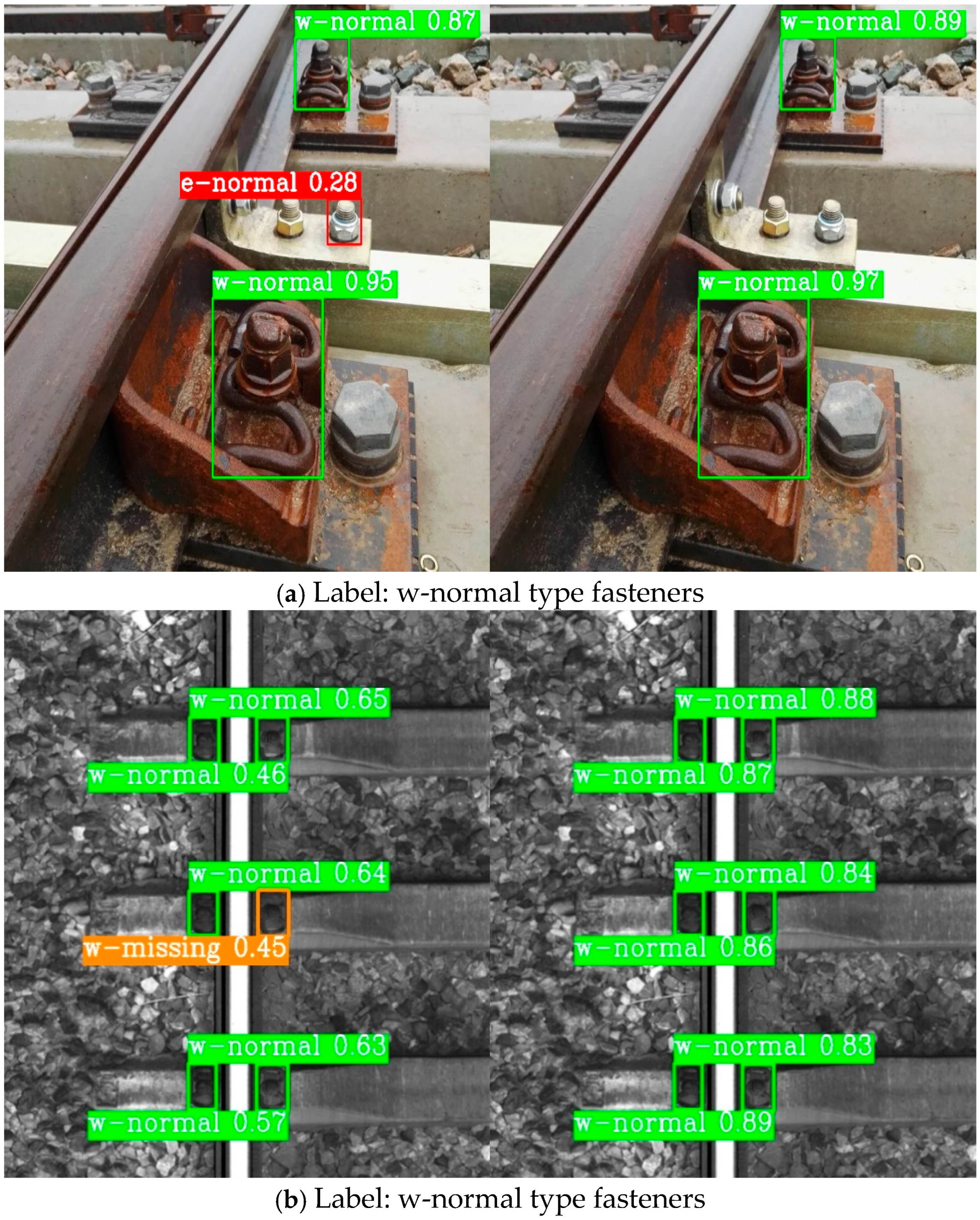
To intuitively demonstrate the superiority of the improved model proposed in this paper in terms of detection performance, a visual comparison of the detection results between the original YOLOv8n model and the YOLOv8n-FDD model on the test set is presented here. The specific results are shown in Figure 15, where the left and right images represent the detection results of the YOLOv8n model and the YOLOv8n-FDD model, respectively.

Specifically, it can be observed in Figure 15a that when detecting w-normal fasteners, the YOLOv8n model exhibits false detections, mistakenly identifying a bolt located outside the fastener position as an e-normal fastener. Similarly, in Figure 15b, the YOLOv8n model once again misclassifies a w-normal fastener as a w-missing fastener, revealing its limitations in distinguishing similar objects against complex backgrounds. 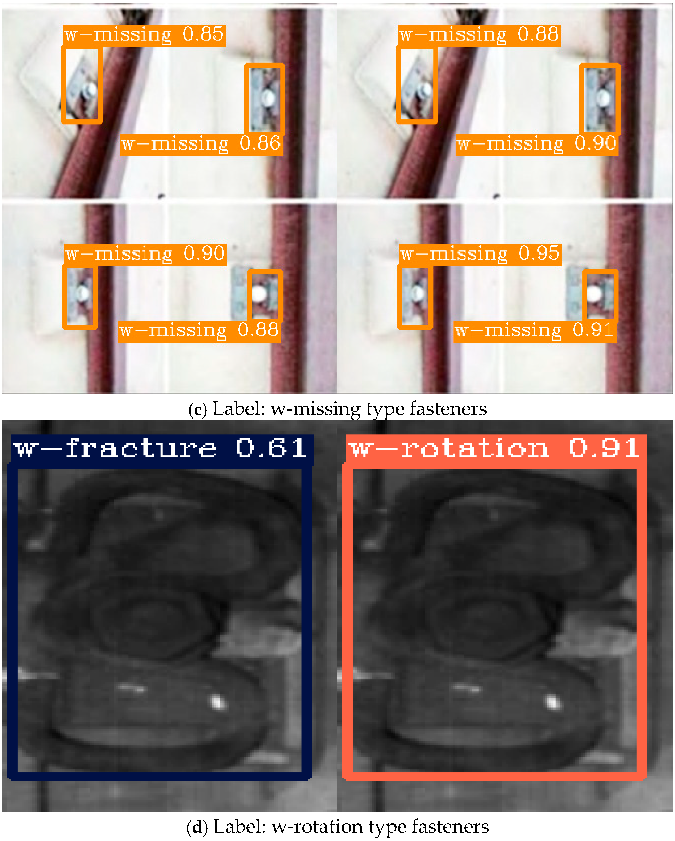In contrast, in Figure 15c, when detecting w-missing fasteners, both models are able to achieve accurate recognition and localization, but the YOLOv8n-FDD model outputs a higher confidence level, demonstrating its superior detection certainty and robustness. Lastly, in Figure 15d, when detecting a w-rotation fastener with rotated morphology, the YOLOv8n model again experiences a false detection, incorrectly identifying it as a w-fracture fastener. Conversely, the YOLOv8n-FDD model accurately recognizes the w-rotation fasteners, indicating its superior feature extraction and adaptability.

In summary, for the detection of different types of fastener defects, the proposed improved model YOLOv8n-FDD exhibits lower false detection rate, higher classification accuracy, and stronger robustness compared to the original YOLOv8n model.

5. Concluding Remarks

This paper focuses on the task of fastener defect detection. By selecting the current advanced object detection model, YOLOv8n, and improving upon it, a YOLOv8n-FDD model specifically designed for fastener defect detection is proposed and the high accuracy and real-time detection of various types of fastener defects is conducted.

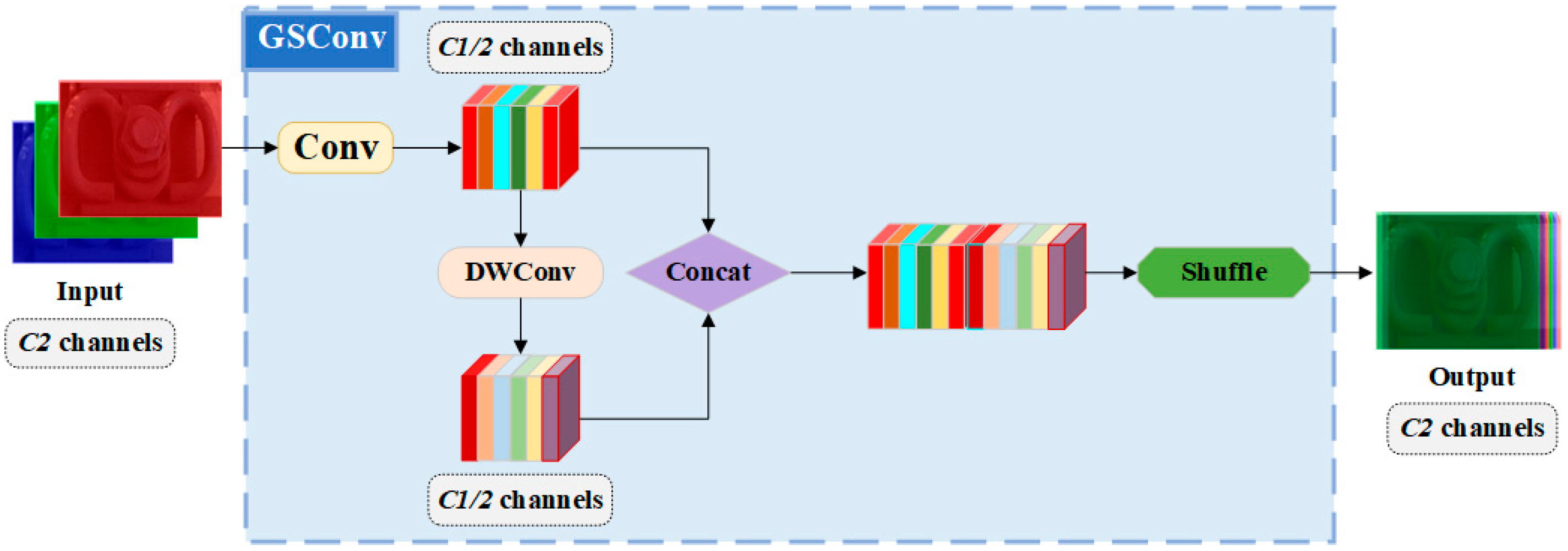
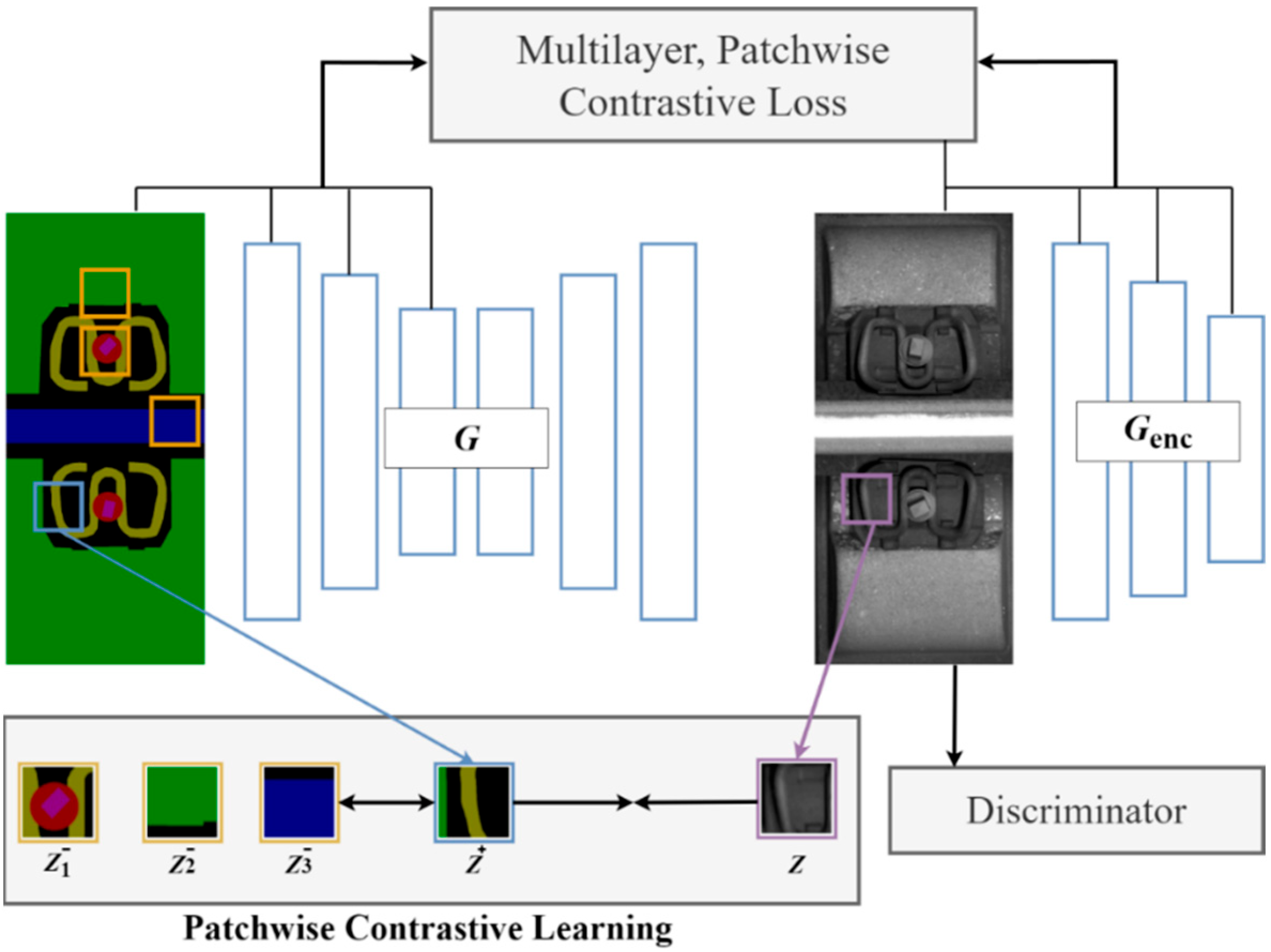
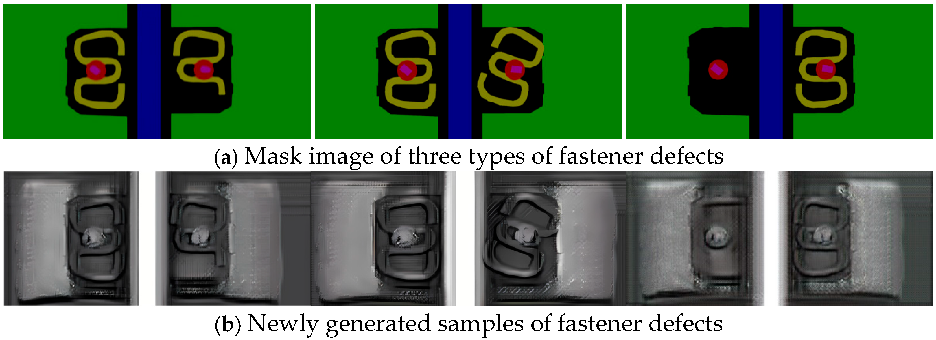
Firstly, to enhance detection accuracy, the CA mechanism is incorporated into the backbone structure of the original YOLOv8n model, thereby optimizing detection performance. Secondly, with respect to the detection efficiency, the traditional Conv module in the backbone structure and the c2f module in the neck structure of the YOLOv8n model are, respectively, replaced with the GSConv and VoVGSPCP modules, effectively reducing the computational complexity of the YOLOv8n-FDD model and achieving model lightweighting. Finally, by upgrading the bounding box loss function of the YOLOv8n model from CIoU to WIoU, the YOLOv8n-FDD model’s generalization ability and overall detection performance in handling complex scenarios are further improved. Additionally, a fastener dataset containing two types of normal fasteners and four types of defective fasteners is established and subsequently preprocessed by the fastener defect sample generation strategy based on the CUT style transfer model, effectively addressing the issue of imbalance distribution in sample categories.

Through comparative experimental validation, the addition of the CA mechanism and the selection of WIoU as the bounding box loss function both contribute to an improvement in detection accuracy compared to the YOLOv8n model. Meanwhile, the introduction of the GSConv and VoVGSPCP modules optimizes the detection speed while reducing both the model size and computational complexity. When benchmarked against other mainstream object detection models, the proposed improved model exhibits superior performance across key metrics. Specifically, the YOLOv8n-FDD model achieves a mAP of 96.1%, a throughput of 91 FPS, a model size of 6 MB, and a computational complexity of 7.4 billion FLOPs.

References

1. Xu, L.; Gao, J.; Zhai, W. On effects of rail fastener failure on vehicle/track interactions. Struct. Eng. Mech. 2017, 63, 659–667. [Google Scholar]
2. Sadeghi, J.; Seyedkazemi, M.; Khajehdezfuly, A. Nonlinear simulation of vertical behavior of railway fastening system. Eng. Struct. 2020, 209, 110340. [Google Scholar] [CrossRef]
3. Yuan, X.; Zhu, S.; Zhai, W. Dynamic performance evaluation of rail fastening system based on a refined vehicle-track coupled dynamics model. Veh. Syst. Dyn. 2021, 60, 2564–2586. [Google Scholar] [CrossRef]
4. Wang, P.; Lu, J.; Zhao, C.; Chen, M.; Xing, M. Numerical investigation of the fatigue performance of elastic rail clips considering rail corrugation and dynamic axle load. Proc. Inst. Mech. Eng. Part F J. Rail Rapid Transit. 2020, 235, 339–352. [Google Scholar] [CrossRef]
5. Yuan, Z.; Zhu, S.; Yuan, X.; Zhai, W. Vibration-based damage detection of rail fastener clip using convolutional neural network: Experiment and simulation. Eng. Fail. Anal. 2021, 119, 104906. [Google Scholar] [CrossRef]
6. Oregui, M.; Li, S.; Núñez, A.; Li, Z.; Carroll, R.; Dollevoet, R. Monitoring bolt tightness of rail joints using axle box acceleration measurements. Struct. Control Health Monit. 2016, 24, e1848. [Google Scholar] [CrossRef]
7. Li, S.; Jin, L.; Jiang, J.; Wang, H.; Nan, Q.; Sun, L. Looseness identification of track fasteners based on ultra-weak FBG sensing technology and convolutional autoencoder network. Sensors 2022, 22, 5653. [Google Scholar] [CrossRef]
8. Zhu, S.; Cai, C.; Spanos, P. A nonlinear and fractional derivative viscoelastic model for rail pads in the dynamic analysis of coupled vehicle–slab track systems. J. Sound Vib. 2015, 335, 304–320. [Google Scholar] [CrossRef]
9. Wang, Z.; Wang, S. Research of method for detection of rail fastener defects based on machine vision. In Proceedings of the 4th International Conference on Mechatronics, Materials, Chemistry and Computer Engineering 2015, Xi’an, China, 12–13 December 2015. [Google Scholar]
10. Ma, H.; Min, Y.; Yin, C.; Cheng, T.; Xiao, B.; Yue, B.; Li, X. A real time detection method of track fasteners missing of railway based on machine vision. Int. J. Perform. Eng. 2018, 14, 1190–1200. [Google Scholar] [CrossRef]
11. Hu, Q.; Fang, F.; Yuan, R. Fastener partial looseness identification of the ballastless track by a time-domain Bayesian approach. Adv. Struct. Eng. 2023, 26, 1835–1846. [Google Scholar] [CrossRef]
12. Fan, X.; Jiao, X.; Shuai, M.; Qin, Y.; Chen, J. Application research of image recognition technology based on improved SVM in abnormal monitoring of rail fasteners. J. Comput. Methods Sci. Eng. 2023, 23, 1307–1319. [Google Scholar] [CrossRef]
13. Wang, X.; Li, H.; Yue, X.; Meng, L. A comprehensive survey on object detection YOLO. In Proceedings of the 5th International Symposium on Advanced Technologies and Applications in the Internet of Things, Kusatsu, Japan, 28–29 August 2023; Volume 3459, pp. 77–89. [Google Scholar]
14. Hsieh, C.; Hsu, T.; Huang, W. An online rail track fastener classification system based on YOLO Models. Sensors 2022, 22, 9970. [Google Scholar] [CrossRef]
15. Li, X.; Wang, Q.; Yang, X.; Wang, K.; Zhang, H. Track fastener defect detection model based on improved YOLOv5s. Sensors 2023, 23, 6457. [Google Scholar] [CrossRef]
16. Cai, Y.; He, M.; Tao, Q.; Xiao, J.; Zhong, F.; Zhou, H. Fast rail fastener screw detection for vision-based fastener screw maintenance robot using deep learning. Appl. Sci. 2024, 14, 3716. [Google Scholar] [CrossRef]
17. Du, L.; Zhang, R.; Wang, X. Overview of two-stage object detection algorithms. J. Phys. Conf. Ser. 2020, 1544, 012033. [Google Scholar] [CrossRef]
18. Bai, T.; Yang, J.; Xu, G.; Yao, D. An optimized railway fastener detection method based on modified Faster R-CNN. Measurement 2021, 182, 109742. [Google Scholar] [CrossRef]
19. Shang, Z.; Li, L.; Zheng, S.; Mao, Y.; Shi, R. FIQ: A fastener inspection and quantization method based on mask FRCN. Appl. Sci. 2024, 14, 5267. [Google Scholar] [CrossRef]
20. Wang, Y.; Ren, B. Quadrotor-enabled autonomous parking occupancy detection. In Proceedings of the IEEE International Conference on Intelligent Robots and Systems, Las Vegas, NV, USA, 25–29 October 2020; pp. 8287–8292. [Google Scholar]
21. Tan, L.; Lv, X.; Lian, X.; Wang, G. YOLOv4_Drone: UAV image target detection based on an improved YOLOv4 algorithm. Comput. Electr. Eng. 2021, 93, 107261. [Google Scholar] [CrossRef]
22. Hussain, M. YOLOv1 to v8: Unveiling each variant-a comprehensive review of YOLO. IEEE Access 2024, 12, 42816–42833. [Google Scholar] [CrossRef]
23. Jin, Y.; Tian, X.; Zhang, Z.; Liu, P.; Tang, X. C2F: An effective coarse-to-fine network for video summarization. Image Vis. Comput. 2024, 144, 104962. [Google Scholar] [CrossRef]
24. Dong, X.; Li, S.; Zhang, J. YOLOV5s object detection based on Sim SPPF hybrid pooling. Optoelectron. Lett. 2024, 20, 367–371. [Google Scholar] [CrossRef]
25. Sharma, D. Information measure computation and its impact in MI COCO dataset. In Proceedings of the 7th International Conference on Advanced Computing & Communication Systems, Coimbatore, India, 19–20 March 2021; pp. 1964–1969. [Google Scholar]
26. Hou, Q.; Zhou, D.; Feng, J. Coordinate attention for efficient mobile network design. In Proceedings of the IEEE Computer Society Conference on Computer Vision and Pattern Recognition, Nashville, TN, USA, 20–25 June 2021; pp. 13708–13717. [Google Scholar]
27. Li, H.; Li, J.; Wei, H.; Liu, Z.; Zhan, Z.; Ren, Q. Slim-neck by GSConv: A better design paradigm of detector architectures for autonomous vehicles. arXiv 2024, arXiv:2206.02424. [Google Scholar]
28. Du, S.; Zhang, B.; Zhang, P.; Xiao, P. An improved bounding box regression loss function based on CIOU loss for multi-scale object detection. In Proceedings of the IEEE 2nd International Conference on Pattern Recognition and Machine Learning, Chengdu, China, 16–18 July 2021; pp. 92–98. [Google Scholar]
29. Tong, Z.; Chen, Y.; Xu, Z.; Yu, R. Wise-IoU: Bounding box regression loss with Dynamic focusing mechanism. arXiv 2023, arXiv:2301.10051. [Google Scholar]
30. Ioffe, S.; Szegedy, C. Batch normalization: Accelerating deep network training by reducing internal covariate shift. In Proceedings of the 32nd International Conference on Machine Learning, Lille, France, 6–11 July 2015; pp. 448–456. [Google Scholar]
31. Misra, D. Mish: A self regularized non-monotonic activation function. arXiv 2019, arXiv:1908.08681. [Google Scholar]
32. Walt, S.; Colbert, S.; Varoquaux, G. The NumPy array: A structure for efficient numerical computation. Comput. Sci. Eng. 2011, 13, 22–30. [Google Scholar] [CrossRef]
33. Hannun, A.; Lee, A.; Xu, Q.; Collobert, R. Sequence-to-sequence speech recognition with time-depth separable convolutions. arXiv 2019, arXiv:1904.02619. [Google Scholar]
34. Iqbal, I.; Odesanmi, G.; Wang, J.; Liu, L. Comparative investigation of learning algorithms for image classification with small dataset. Appl. Artif. Intell. 2021, 35, 697–716. [Google Scholar] [CrossRef]
35. Byun, J.; Cha, S.; Moon, T. Fbi-denoiser: Fast blind image denoiser for poisson-gaussian noise. In Proceedings of the IEEE Conference on Computer Vision and Pattern Recognition, Nashville, TN, USA, 20–25 June 2021; pp. 5768–5777. [Google Scholar]
36. Kumain, S.; Kumar, K. Quantifying salt and pepper noise using deep convolutional neural network. J. Inst. Eng. Ser. B 2022, 103, 1293–1303. [Google Scholar] [CrossRef]
37. Li, C.; Zhu, J.; Bi, L.; Zhang, W.; Liu, Y. A low-light image enhancement method with brightness balance and detail preservation. PLoS ONE 2022, 17, e0262478. [Google Scholar] [CrossRef]
38. Qiu, S.; Cai, B.; Wang, W.; Wang, j.; Zaheer, Q.; Liu, X.; Hu, W.; Peng, J. Automated detection of railway defective fasteners based on YOLOv8-FAM and synthetic data using style transfer. Autom. Constr. 2024, 162, 105363. [Google Scholar] [CrossRef]
39. Park, T.; Efros, A.; Zhang, R.; Zhu, J. Contrastive learning for unpaired image-to-image translation. In Proceedings of the Computer Vision-ECCV 2020: 16th European Conference, Glasgow, UK, 23–28 August 2020; pp. 319–345. [Google Scholar]
40. Brooks, T.; Holynski, A.; Efros, A. InstructPix2Pix: Learning to follow image editing instructions. In Proceedings of the IEEE Computer Society Conference on Computer Vision and Pattern Recognition, Vancouver, BC, Canada, 17–24 June 2023; pp. 18392–18402. [Google Scholar]
41. Tan, H.; Liu, X.; Yin, B.; Li, X. MHSA-Net: Multihead self-attention network for occluded person re-identification. IEEE Trans. Neural Netw. Learn. Syst. 2022, 34, 8210–8224. [Google Scholar] [CrossRef] [PubMed]
42. Yang, J.; Jiang, J. Dilated-CBAM: An efficient attention network with dilated convolution. In Proceedings of the IEEE International Conference on Unmanned Systems, Beijing, China, 27–28 November 2021; pp. 11–15. [Google Scholar]
43. Zheng, Z.; Wang, P.; Liu, W.; Li, J.; Ye, R.; Ren, D. Distance-IoU loss: Faster and better learning for bounding box regression. Proc. AAAI Conf. Artif. Intell. 2020, 34, 12993–13000. [Google Scholar] [CrossRef]
44. Zhang, Y.; Ren, W.; Zhang, Z.; Jia, Z.; Wang, L.; Tan, T. Focal and efficient IOU loss for accurate bounding box regression. Neurocomputing 2022, 506, 146–157. [Google Scholar] [CrossRef]
45. Liu, W.; Anguelov, D.; Erhan, D.; Szegedy, C.; Reed, S.; Fu, C.; Berg, A. SSD: Single shot multibox detector. In Proceedings of the European Conference on Computer Vision, Amsterdam, The Netherlands, 11–14 October 2016; Volume 9905, pp. 21–37. [Google Scholar]
46. Everingham, M.; Gool, L.; Williams, C.; Winn, J.; Zisserman, A. The pascal visual object classes (voc) challenge. Int. J. Comput. Vision. 2010, 88, 303–338. [Google Scholar] [CrossRef]
Figure 1. Schematic diagram of the composition of rail fasteners.
Machines 13 00511 g001
Figure 2. The original YOLOv8n model architecture.
Machines 13 00511 g002
Figure 3. Optimized YOLOv8n-FDD model architecture.
Machines 13 00511 g003
Figure 4. Structure of the CA mechanism.
Machines 13 00511 g004
Figure 5. Schematic diagram of average pooling in height and width dimensions.
Machines 13 00511 g005
Figure 6. Schematic diagram of the concatenated feature map.
Machines 13 00511 g006
Figure 7. Structure of the GSConv module.
Machines 13 00511 g007
Figure 8. Structure of the VoVGSPCP module.
Machines 13 00511 g008
Figure 9. The service status types of fasteners included in the dataset.
Machines 13 00511 g009
Figure 10. Visualization of data augmentation effects.
Machines 13 00511 g010
Figure 11. Schematic diagram of fastener defect sample generation based on the CUT style transfer model.
Machines 13 00511 g011
Figure 12. Comparison before and after the generation of fastener defect samples.
Machines 13 00511 g012
Figure 13. Training process of the YOLOv8n model and YOLOv8n-FDD model.
Machines 13 00511 g013
Figure 14. Comparison of detection accuracy of the YOLOv8n-FDD model for different types of fastener defects.
Machines 13 00511 g014
Figure 15. Detection results of different types of fastener defects (left: YOLOv8n model; right: YOLOv8n-FDD model).
Machines 13 00511 g015aMachines 13 00511 g015b