Article

Gear Target Detection and Fault Diagnosis System Based on Hierarchical Annotation Training

1
College of Electrical Engineering and Automation, Fuzhou University, Fuzhou 350000, China
2
The Key Laboratory of Industrial Automation Control Technology and Information Processing, Education Department of Fujian Province, Fuzhou 350000, China
3
School of Information and Electrical Engineering, Hunan University of Science and Technology, Xiangtan 411201, China
4
Division of Industrial Data Science, School of Data Science, Lingnan University, Hong Kong, China
5
IAP (Fujian) Technology Co., Ltd., Fuzhou 350116, China
*
Author to whom correspondence should be addressed.
Machines 2025, 13(10), 893; https://doi.org/10.3390/machines13100893
Submission received: 1 September 2025 / Revised: 27 September 2025 / Accepted: 28 September 2025 / Published: 30 September 2025
(This article belongs to the Section Machines Testing and Maintenance)

Abstract

Gears are the core components of transmission systems, and their health status is critical to the safety and stability of the entire system. In order to efficiently identify the typical fault types such as missing teeth and broken teeth in gears, this paper collects a rich sample under complex backgrounds from different shooting angles and lighting conditions. Then a hierarchical approach is used to describe gear faults on the image. The gear samples are first segmented for image extraction and then finely labeled for gear fault regions. In addition, imbalanced datasets are produced to simulate the environment with fewer fault samples in the actual industrial process. Finally, a semi-supervised learning framework is trained based on the above method and applied in actual environment. The experimental results show that the model performs well in gear target detection and fault diagnosis, demonstrating the effectiveness of the proposed method.

1. Introduction

In modern industrial processes, as mechanical equipment becomes increasingly complex and automation levels rise [1], gears are widely used as core transmission components in high-end intelligent manufacturing fields such as automobile, aerospace, shipbuilding and rail transit [2]. Therefore, the working status of gears will directly affect the overall performance of the equipment. Due to various problems such as changes in loads and external impacts during long-term operation, gears are prone to faults such as missing teeth and broken teeth [3]. If these faults are not detected and investigated in a timely manner, it will not only reduce the operating efficiency of the equipment, but also cause equipment shutdown and damage, leading to safety accidents and huge economic losses.
Hence, gear fault diagnosis has been an important research direction in the industrial field [4]. Traditional manual detection is time-consuming and labor-intensive, and no longer meets the efficiency requirements of the intelligent manufacturing industry. Signal analysis based on sensors effectively improves detection efficiency and is a common diagnostic method. Xiao et al. [5] use a phonon crystal resonator with directional enhancement capabilities for acoustic signals to identify fault categories by analyzing the acoustic signals of gears. Similarly, spectral analysis is used for fault diagnosis. A blind deconvolution strategy based on spectral kurtosis is proposed, which performs gear fault detection by filtering in the order domain [6]. However, methods based on signal analysis are easily affected by noise when extracting fault features and have certain limitations in practical applications.
Currently, fault diagnosis techniques are categorized into mechanism-based methods and data-driven methods [7]. In terms of mechanism-based methods, a gear crack propagation model is constructed for dynamic simulation to extract fault characteristics [8]. However, due to the insignificant change of early crack propagation in gears, this method is unable to identify faults in time when they occur. To improve the real-time performance and accuracy of fault diagnosis, Dadon et al. [9] propose a new general model of gear dynamics that analyzes the effect of faults on meshing stiffness to simulate common tooth surface defects. Although mechanism modeling methods accurately reflect the dynamic behavior of real systems, the complexity of physical structures and the large computational requirements limit the widespread use of this method.
With the development of machine learning, the fault diagnosis methods based on data modeling have demonstrated powerful capabilities in complex industrial systems [10]. Deep learning has become the foundation for most data-driven fault diagnosis methods due to its ability to better extract underlying features from complex data [11]. Currently popular deep learning models such as convolutional neural networks, long short-term memory networks, graph neural networks and autoencoders have been successfully applied to gear fault identification and have achieved remarkable results [12,13,14]. For example, Heydarzadeh et al. [15] use detection signals in the discrete wavelet domain as input for a deep neural network to diagnose transmission gear faults. Saufi et al. [16] develop a fault diagnosis system based on time-frequency image pattern recognition using stacked sparse autoencoders. However, these methods have high requirements for data balance distribution. In fact, the number of fault samples is much smaller than the number of normal samples [17], making it extremely difficult for the model to capture fault features during training, resulting in false positives and false negatives.
To solve the problem of imbalanced data, traditional oversampling tends to repeat sample noise, resulting in overfitting; while undersampling tends to lose marginal samples, leading to underfitting [18]. In order to optimize traditional sampling methods, Dablain [19] proposes a deep synthesis oversampling technique for minority groups. However, for neighboring samples of different categories, the samples synthesized by this method tend to confuse features. In addition to adjusting the samples, category weights are introduced and integrated with the loss function to strengthen the influence of minority categories on model parameters [20]. However, the setting of category weights depends on experience and the effectiveness of them is limited. Moreover, ensemble learning is also a solution. AdaBoost [21] and Random Forest [22] have been applied to imbalanced data classification problems and have achieved remarkable results. However, existing ensemble learning methods usually rely on strong feature selection, complex model training, and high computational costs [23].
Semi-supervised learning is another approach to mitigating the effects of the imbalanced datasets. Currently, semi-supervised learning is categorized into generative methods, graph-based methods, consistency regularization methods, and pseudo-labeling methods [24]. Generative methods accomplish classification tasks by learning the latent distribution of data through tools such as generative adversarial networks [25]. However, due to the limited amount of labeled data, the training process is less stable. Graph-based methods often incorporate graph neural networks [26], treating samples as nodes and sample similarity as edge weights, thereby assigning identical labels to similar nodes. However, their performance relies on the selection of similarity metric. A classic example of consistency regularization is the teacher–student model [27]. The teacher model provides a more stable target for training of the student model. This approach relies on data augmentation strategies and requires training two models, resulting in high computational costs. Pseudo-labeling methods [28] first train an initial model using the labeled data to assign high-confidence predictions to the unlabeled data, then they are added back to the training set for retraining. However, this approach is prone to accumulating and amplifying errors.
The popular public datasets have balanced sample sizes across all categories and contain images with pure white backgrounds, taken from the same angle and under bright, uniform lighting conditions like Figure 1. This facilitates model training, but images with cluttered backgrounds, tilted shooting angles and shadow interference are very common in actual industrial scenarios. In such cases, models trained by public datasets are likely to experience a decline in accuracy during fault diagnosis because they have not learned gear features under complex environmental conditions. Therefore, this paper collects images of gear samples from different shooting angles and under different lighting conditions in complex environments, and then uses annotation tools to describe gear faults hierarchically. Unlike traditional end-to-end models with weak interpretability in decision-making, where the features for the diagnosis remain unknown, the hierarchical annotation training proposed in this paper provides a clear diagnostic logic. In the first stage, the model extracts the entire gear from complex backgrounds. In the second stage, it locates the faulty area on the gear and then determines the fault type based on this location. Furthermore, three different ratios of imbalance datasets are created. Next, a semi-supervised learning framework that combines convolutional neural networks (CNN) and K-means is trained by using the dataset constructed above. Finally, the trained model is applied to the transmission gear assembly platform, demonstrating excellent performance with high accuracy, precision, and recall. The contributions of this paper are as follows:
1.
Hierarchical training is employed to enhance the gear fault localization capabilities of diagnostic models in complex environments.
2.
Imbalanced datasets are generated for hierarchical annotation, where images are captured under complex backgrounds from varying distances and angles.
3.
The model trained by using the proposed method is applied to actual sites and its excellent performance proves the effectiveness of the method.
The rest of this article is organized as follows. Section 2 describes the data collection and annotation methods as well as the construction of the semi-supervised learning framework. Section 3 conducts the experiments and analyzes the results. Finally, conclusions and future work are presented in Section 4.

2. Methodology

2.1. Data Acquisition

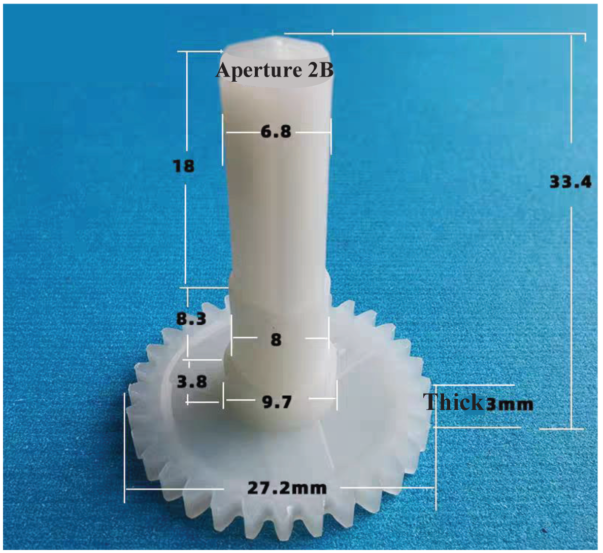
The gear type selected for target detection and fault diagnosis is the 32-teeth hexagonal shaft gear with a connecting rod. The specific dimensions of this gear are shown in Figure 2.
As can be seen from Figure 2, the length of the gear base is only 27.2 mm. Therefore, if a loss or breakage fault occurs on a single gear tooth, the fault area is relatively small. This small local difference places high demands on the feature extraction capabilities of the target detection network. At the same time, due to the 3 mm thickness of the gear profile, if the angle between the camera’s shooting center and the faulty gear is too large, the edge features of the gear are likely to become distorted and blurred, making it easy to confuse the type of gear edge defect. These issues make it difficult for CNNs trained by traditional methods to accurately identify fault types.
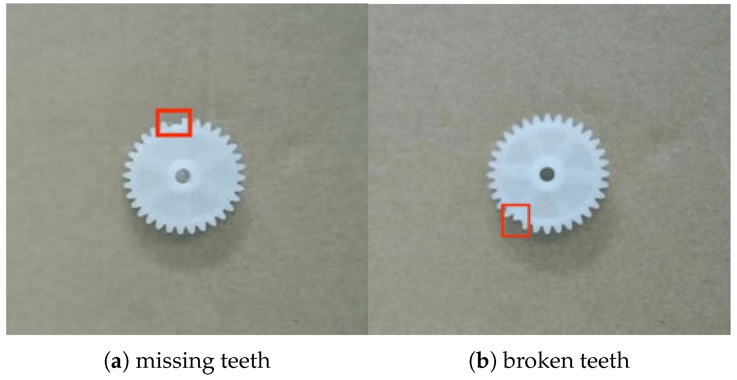
Figure 3 shows a schematic diagram of the faulty gear made from the 32-teeth hexagonal shaft gear. The main faults are missing teeth (Figure 3a) and broken teeth (Figure 3b). Both types of gear faults are common in industrial production, which would cause significant losses in the industrial production process.
Analysis of Figure 3a shows that missing teeth areas typically exhibit characteristics such as discontinuities at the gear edge, local structural defects, and concave contours. Unlike normal gears with periodic contours, missing teeth gears exhibit sudden discontinuities at the boundary. Additionally, the color values and texture characteristics of the missing areas are significantly different from those of the normal teeth sections. As shown in Figure 3b, teeth breakage typically exhibits localized notches or irregular depressions on the teeth tips and teeth surfaces of the gear teeth. Broken-teeth gears differ from normal missing-teeth gears in that the geometric structure of the teeth profile is often irregular, and the crack patterns vary. The surface texture at the broken-teeth location typically exhibits a rough and uneven state, often accompanied by varying degrees of burrs, debris, and microscopic surface fractures.
It can be seen that the image range of fault features are very small. When the gear is placed at a distance close to the camera, an industrial camera that cannot adjust its focus will lose focus, causing the image to be blurred and making it impossible to accurately obtain the gear fault features. When the gear is placed at a distance far from the camera, an industrial camera with low resolution will also be unable to capture clear images of the gear’s edge features. To ensure the quality of gear image acquisition, this paper selects a USB interface camera from RMONCAM as the image acquisition device whose specific parameters are shown in Table 1.
This camera ensures high image clarity and preserves image details. At the same time, the USB interface greatly simplifies the experimental platform setup process and improves deployment efficiency.
Considering that fault features are influenced by shooting conditions, a data collection strategy is employed using different shooting angles, distances, and orientations of gear defects to enhance the diversity and balance of input data for the deep learning model. During the shooting process, the gear samples were fixed on a brown experimental box that could rotate freely and adjust the distance, while the camera was supported by a tripod to maintain a relatively stable acquisition posture. The collected samples included healthy gears, gears with missing teeth, and gears with broken teeth. Considering that gears with the same defect type have differences and diversity in the details of the defect area, each of the three types of gears had ten samples with distinct features. Each gear was placed on the experimental box at different rotation angles to ensure that defects could be captured from all directions of the gear teeth. Additionally, the camera was positioned at different angles relative to the gear center (e.g., −15°, 0°, 15°) and at varying distances (e.g., 20 cm to 60 cm) to obtain a diverse range of gear samples, thereby enhancing the model’s ability to detect changes in the target space. Examples of images under different shooting conditions are presented in Figure 4.

2.2. Hierarchical Annotation

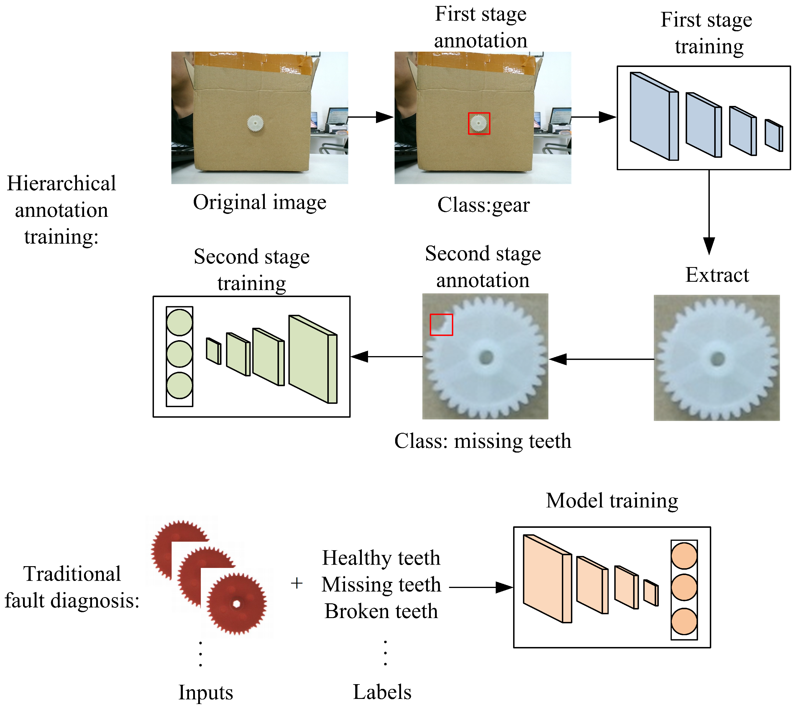
The image acquisition process yields a diverse range of gear samples. However, the shooting environment for the acquisition process is set in a standard indoor workbench area, where the background inevitably includes many irrelevant elements. This factor leads to the raw images containing complex backgrounds and blurred boundaries of the gear targets. If a traditional single-stage object detection process is used, the features on the gear boundaries are confused by background interference. Therefore, improvements to the image annotation strategy are necessary. A hierarchical annotation strategy is employed to describe gear faults, aiming to enhance detection accuracy and system versatility. The first stage focuses on precisely extracting gear targets from complex backgrounds within the overall image, while the second stage concentrates on refined defect identification and classification within the gear images extracted in the first stage.
Both stages of annotation are performed using Labeling software. The annotation format follows the YOLO standard format, with each image corresponding to a .txt file. Each line in the file represents the detection information for a single object, with the data arranged from left to right as follows: the category label of the object, the x and y-coordinate of the center point of the annotation box relative to the image, width and height of the annotation box relative to the image.
In the first stage, sample categories are not distinguished and the annotation box encompasss the entire gear. The model is trained based on the position and size of the annotation box to crop the target gear. The second stage of annotation is based on the single gear subgraphs extracted in the previous stage, but mainly focuses on subgraphs with missing teeth and broken teeth. Healthy gears only need to be categorized, while others also need to be annotated with the local defect areas. For gears with missing teeth, the annotation box should be close to the missing area of the gear edge; while for gears with broken teeth, the annotation box should precisely cover the broken area. Figure 5 illustrates the overall annotation process and demonstrates the difference from traditional approaches where fault samples are directly input into the model.

2.3. Semi-Supervised Learning Framework

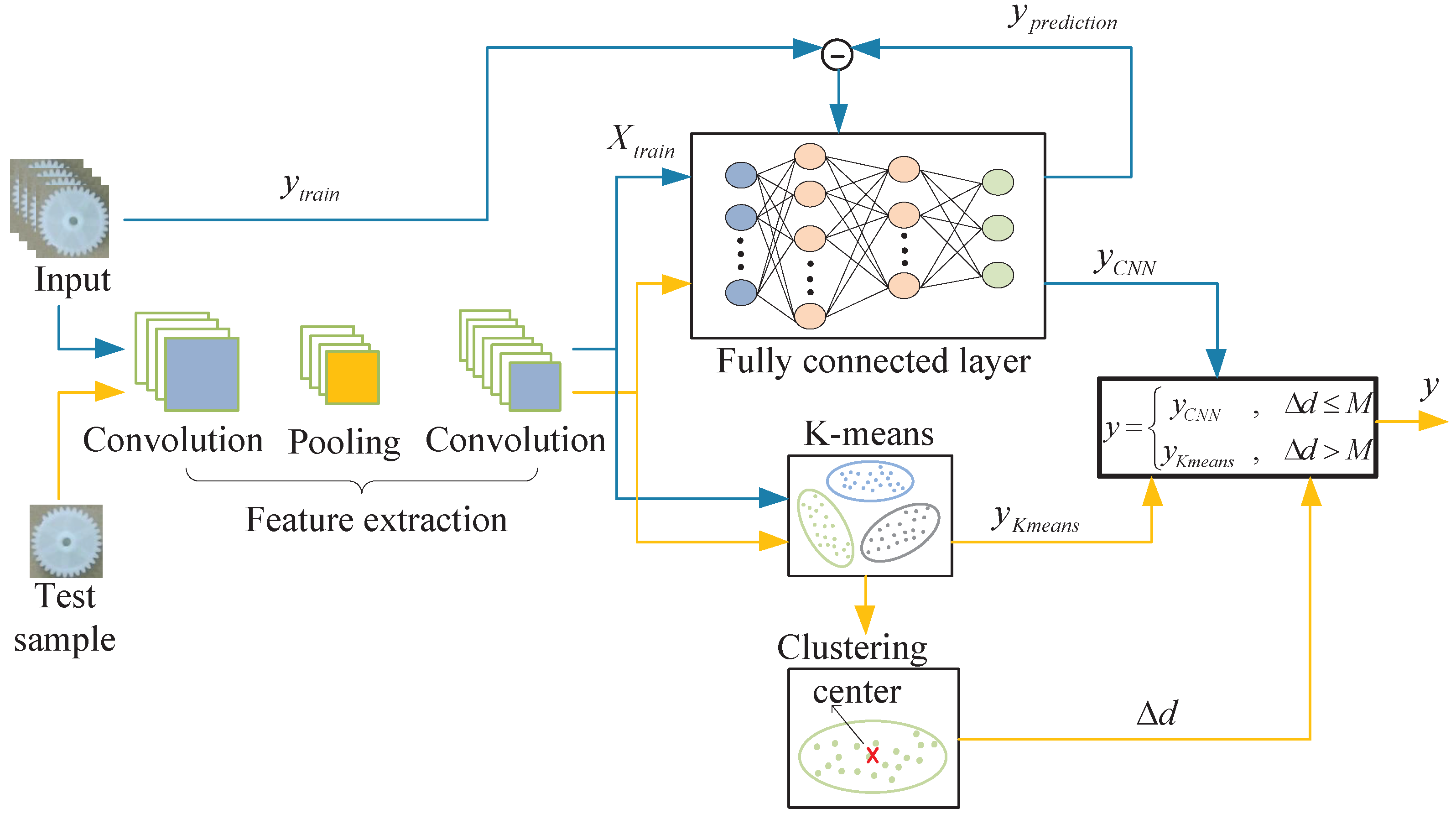
Figure 6 shows the semi-supervised learning framework integrating CNN and K-means.
This framework uses the backbone layer of the YOLOv8 network for feature extraction, obtaining the feature matrix for each training sample. It then clusters the feature matrix using the K-means algorithm to obtain the clustering centers for each type. The feature matrix is then input into the fully connected layers to complete the training for the classification task. During testing, the framework combines the prediction from the CNN with that from K-means and introduces a threshold to make the final decision. The specific decision-making process is as follows: if the CNN and K-means prediction labels are consistent, then the result is directly accepted. Otherwise, a distance metric is introduced for judgment. The Nth testing sample is denoted as x t e s t _ N . The clustering center of the CNN predicted category is C C N N and the clustering center of the K-means predicted category is C K m e a n s . The Euclidean distances d x t e s t _ N , C C N N and d x t e s t _ N , C K m e a n s between the sample and the two clustering centers are calculated. Since the K-means has categorized the sample into a certain type, d x t e s t _ N , C K m e a n s must be less than or equal to d x t e s t _ N , C C N N . However, the K-means algorithm is not very accurate due to the data imbalance and the similarity of features with tiny faults in gears, but the K-means algorithm sometimes predicts accurately in case of wrong prediction by CNN. Thus combining the advantages of both, a threshold M is set for decision making based on the difference between the two distances. When the difference between the two distances is not significant, the CNN prediction with higher accuracy is more convincing. Therefore, if Equation (1) is satisfied, the CNN prediction is used; otherwise the result of K-means is adopted.
d x t e s t _ N , C C N N d x t e s t _ N , C K m e a n s M .

3. Experimentation

3.1. Preparation

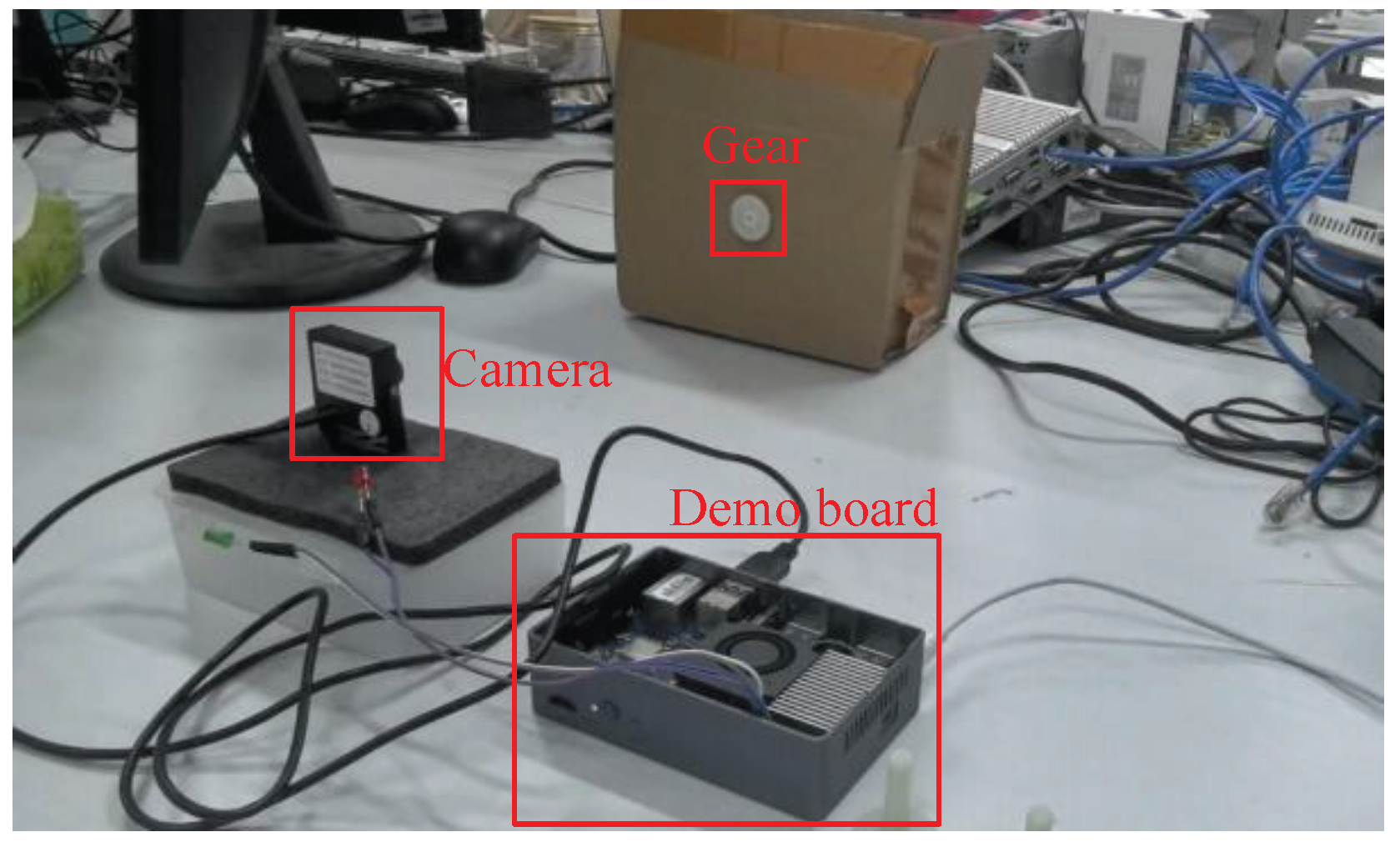
A total of 400 pictures of each type of gears are taken with the RMONCAM camera (RMONCAM, Shenzhen, China). Mirror flip, contrast enhancement, and image center rotation are performed to expand the three types of gears to 1200 pictures respectively. Different numbers of pictures are randomly selected and annotated to create the imbalanced datasets. A total of 500 images of normal gears are randomly selected and a corresponding number of images of the two types of faulty gears are selected and annotated according to different degrees of imbalance. The details of the self-constructed imbalanced datasets are presented in Table 2. After training is complete, the models are deployed on the OrangePi AI Pro demo board (OrangePi, Shenzhen, China) in ONNX format to enable real-time image capture and fault diagnosis tasks. The experimental detection platform is shown in Figure 7.
The testing is conducted on 30 gears with different characteristics, including 10 gears with missing teeth, 10 gears with broken teeth, and 10 normal gears. Each faulty gear exhibits distinct defect characteristics. Each model trained on an imbalance dataset is tested 100 times, with 35 tests on gears with missing teeth or broken teeth and 30 tests on normal gears. The gears are randomly selected and placed on the box at random rotation angles. The test metrics are accuracy, precision and recall, as shown in Equations (2)–(4).
Accuracy = T P + T N T P + F N + F P + T N ,
Precision = T P T P + F P ,
Recall = T P T P + F N ,
where T P , T N , F P , F N are true positive, true negative, false positive and false negative, respectively.

3.2. Hierarchical Training

In the experiment, YOLOv8s is selected as the training model [29]. Since the hierarchical annotation is used, the hierarchical training is also adopted. Each dataset is divided into training and validation sets in an 8:2 ratio. Input images are uniformly scaled to a size of 640 × 640 pixels. The initial learning rate and final learning rate are both set to 0.01, and the training batch size is set to 16. The weights for the target box regression loss, classification loss, and distributed focus loss are fine-tuned near their default values. Since metrics decline on the validation set, the default weights for all three losses are adopted. They are 7.5, 0.5, and 1.5, respectively. Various data augmentation techniques such as random image translation, scaling and color perturbation are enabled. The pre-trained weights of the YOLOv8s on the large-scale public dataset COCO (https://cocodataset.org (accessed on 24 July 2025)) are loaded. This setting improves the generalization of this model across different task environments. During the validation, in addition to precision and recall, mAP50 and mAP50-95 are also employed as metrics. The calculation for mAP is shown in Equation (5).
mAP = 1 N i = 1 N A P i ,
where N is the total number of categories. A P i represents the average precision for ith category, which is essentially the area under the curve formed by the precision and recall axes. mAP50 and mAP50-95 introduce a threshold for the intersection of union (IoU) between predicted and true bounding boxes based on mAP. The definition of IoU is shown in Equation (6).
IoU = S p r e S t r u e S p r e S t r u e ,
where S p r e and S t r u e represent the area of the predicted box and the true box respectively. When IoU exceeds the set threshold, the predicted category is considered correct. mAP50 is the mAP value calculated at a threshold of 0.5, as shown in Equation (7). Within the range from 0.5 to 0.95, 10 thresholds are selected at intervals of 0.05. The mAP value is computed at each threshold, and the average is denoted as mAP50-95, as shown in Equation (8).
mAP50 = mAP 0.5 = 1 N i = 1 N A P i 0.5 ,
mAP50-95 = 1 10 i = 0 9 mAP 0.5 + 0.05 i ,
where mAP k denotes the mAP value at threshold k and A P i 0.5 is the average precision for ith category when the threshold is 0.5.
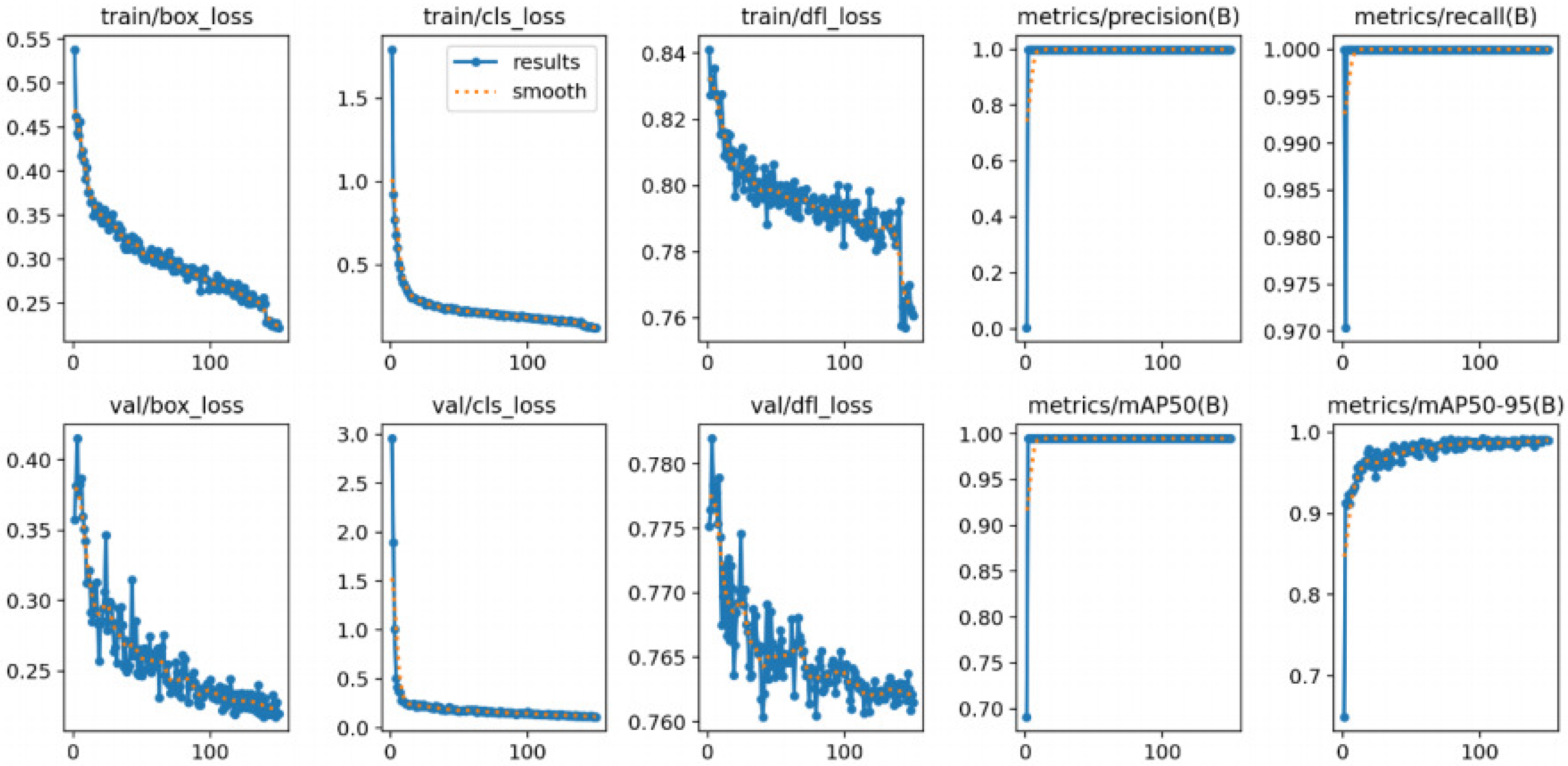
Since the training targets of two stages are not the same, the epochs for two stages is set differently. Using a dataset with an imbalance ratio of 5:1:1 as an example, the training results in the first stage when the epochs is set to 150 are shown in Figure 8. The smoothing in the figure are achieved by using a one-dimensional Gaussian filter with a standard deviation of 3. As shown in the figure, the three loss functions during training and validation all decrease gradually from a relatively high value, indicating that the accuracy and distribution quality of the target boxes are gradually improving. Additionally, the loss function decreases steadily and does not increase in the later epochs, proving that the risk of overfitting is low. The precision, recall, and mAP50 all approach 1.0 and reach saturation after 10 training rounds, while the mAP50-95 also gradually increases and approaches 0.99, proving that the model has virtually no false negatives or false positives. Therefore, it can be concluded that when the epochs is set to 150, the model has strong detection capabilities for gear targets and can proceed to the second stage of training.
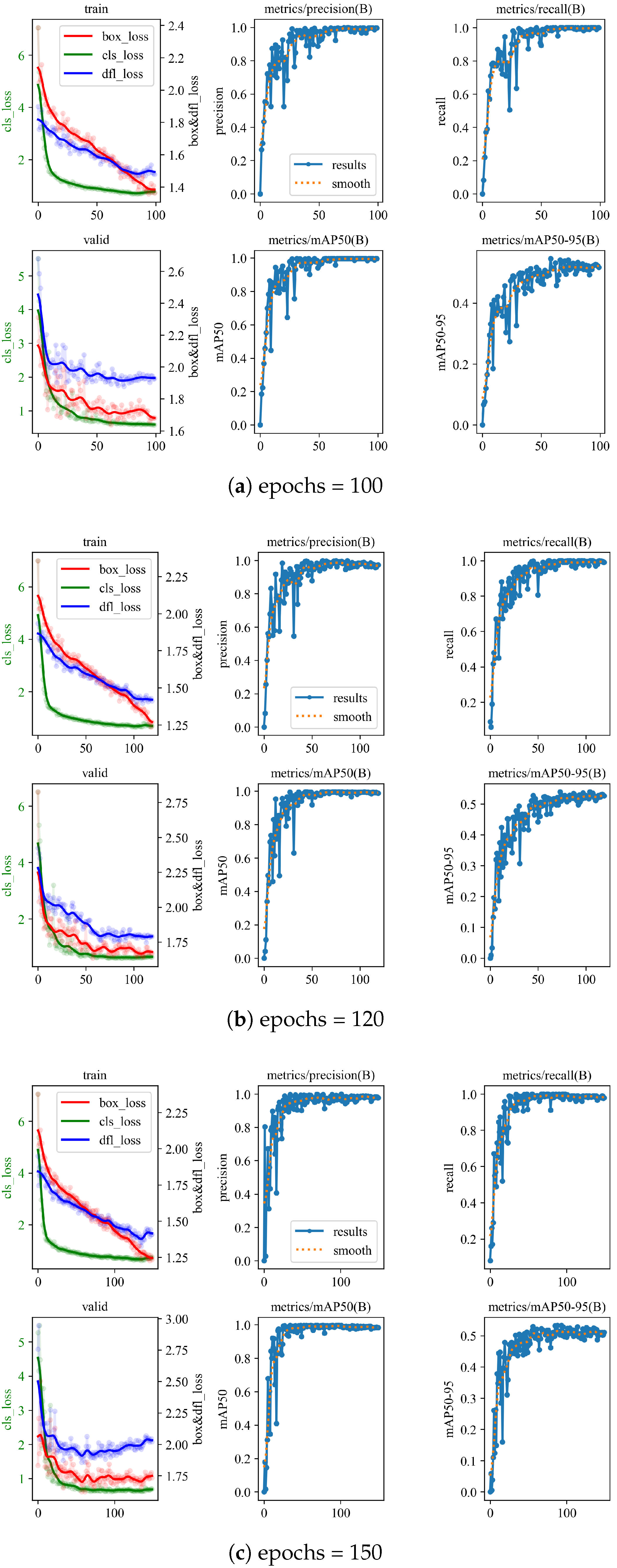
In the second stage, the training results across different epochs are shown in Figure 9. As seen in Figure 9a,b, the three loss curves on the validation set exhibit a declining trend before epoch 50, followed by relative stability. In Figure 9c, the loss curves show an upward trend toward the end, indicating that the model has overfitted and requires early stopping. All four metrics show some fluctuations, suggesting that the model experiences minor detection confusion between missing teeth and broken teeth. The fluctuations of the four metrics in Figure 9a are more pronounced compared to those in Figure 9b. To ensure the accuracy of the second stage model training, the weight file in 120 epochs is saved.
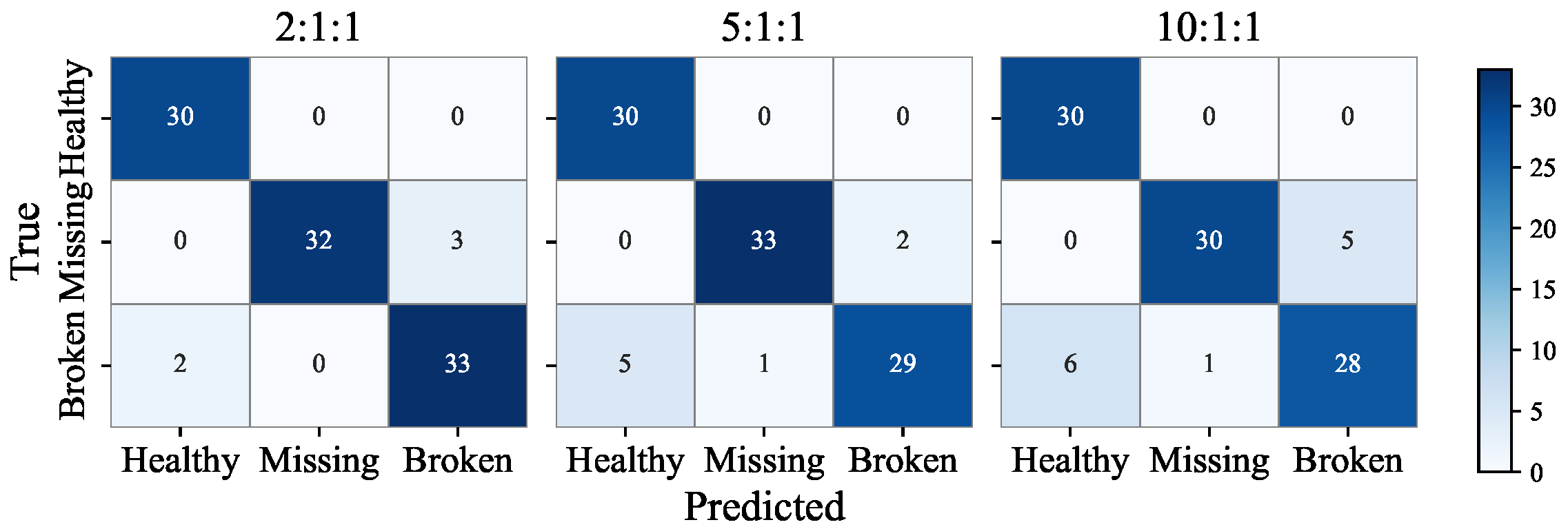
The test results of each model trained with unbalanced data are shown in Figure 10, and the metrics are presented in Table 3. As can be seen from the results, the accuracy of the system shows a decreasing trend as the imbalance of the dataset increases. The system tends to classify minority fault samples as healthy samples. When the imbalance ratio is 2:1:1, the overall performance of the system is balanced, and the model can adequately learn from all types of samples. As imbalance increases, the system generates more false positives for the broken tooth category, indicating that the increased proportion of healthy gear samples in the dataset reduces the ability of the model to learn fault features of small-category samples. Under the influence of severe imbalance, the model prioritizes the identification of majority-category samples while neglecting minority-category samples, leading to a degradation in the model’s detection and diagnostic capabilities.

3.3. Semi-Supervised Learning Framework

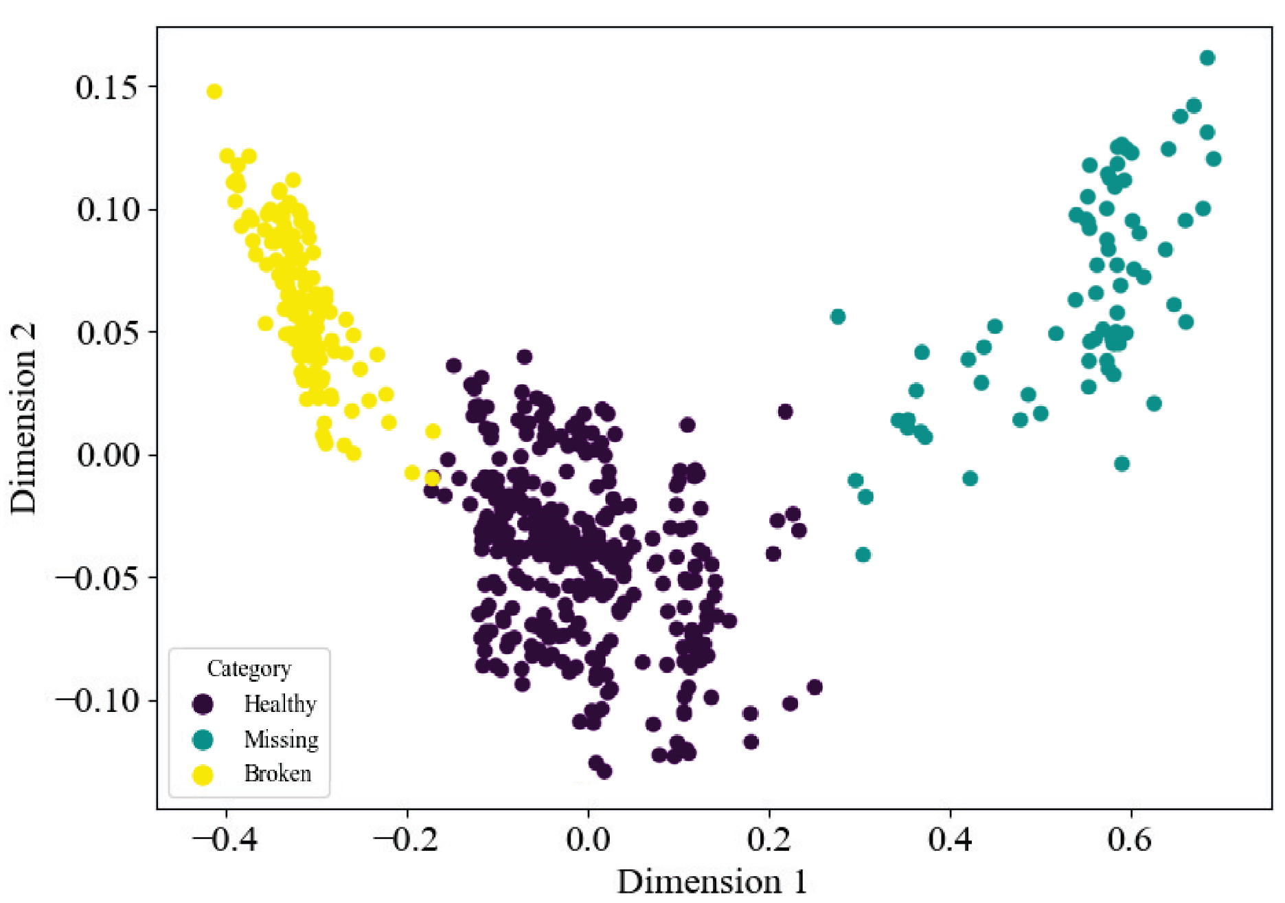
The subgraphs cut out in the second stage are used as inputs for the framework. Images are uniformly scaled to 640 × 640 pixels, and each image label is described in a .csv file, where the first and second columns are the image file names and gear categories, respectively, for supervising the training of the CNN part. The number of cluster categories is set to 3, corresponding to gears with missing, broken, and healthy teeth. To more intuitively evaluate the classification ability of the clustering model, t-SNE is used to reduce the high-dimensional features to a two-dimensional space for visualization. Taking the training results with an imbalance ratio of 5:1:1 as an example, the visualization is shown in Figure 11. It can be observed that the three types of data exhibit distinct separability in the feature space, with each type forming a clear and independent cluster within the feature space. However, similar to the fault features analyzed earlier, the edges of the broken teeth become blurred at certain angles, leading to the broken gear being misclassified as a healthy gear. In the visualization results, the cluster containing the broken gear still overlaps partially with the cluster containing the healthy gears, which would easily cause misclassification during testing. Missing-teeth gears, due to their more pronounced fault features and significant differences in features, exhibit greater distances between samples in the feature space.
The value of threshold M is selected during the training by utilizing the validation set. The test results of the models trained on each imbalanced dataset are shown in Table 4.
The test data shows that the accuracy of this system decreases under a 2:1:1 imbalance ratio compared with the supervised framework, while the accuracy improves under the other two imbalance ratios. From the dimension-reduced space, some sample points of broken teeth and normal categories overlap. When the imbalance is small, more overlapping points occur, causing the system to misclassify broken teeth as normal, thereby reducing overall accuracy. Conversely, as imbalance increases, overlapping points decrease, leading to fewer misclassifications and improved accuracy. The system performs well for the healthy and missing categories, achieving a recall of 1.0 for the healthy category, indicating that no errors occur in classifying actual healthy gears. For the missing category, the system performs stably overall, with precision and recall rates maintaining above 0.88 under various imbalance conditions. Especially under a 5:1:1 imbalance ratio, the missing category exhibits high precision and recall, demonstrating that the K-means can assist decision-making to some extent and effectively enhance the feature recognition capabilities. In contrast, the system still faces challenges in classifying the broken category. Although all metrics remain above 0.82, the recall for the broken category decreases as the imbalance increases. This reflects that broken teeth samples have less distinct features and are more easily overshadowed by the healthy category, leading to overlapping or blurred the clustering boundary and thereby affecting the final decision.

3.4. Comparison

To validate the superiority of the proposed method, the two frameworks are trained using public datasets without hierarchical annotation and their test results are compared. The public dataset is from Roboflow (https://universe.roboflow.com/gear-u48i0/gear-defect (accessed on 24 July 2025)). The experimental environment, training hyperparameters and the threshold of the semi-supervised learning framework remained unchanged. The geometric mean accuracy (G-mean) [30] is used as the metric, as shown in Equation (9).
G - mean = i = 1 m P r e i 1 m ,
where m is the number of types and P r e i represents the precision of the i-th type.
The G-mean values of detection models trained on different datasets are presented in Table 5.
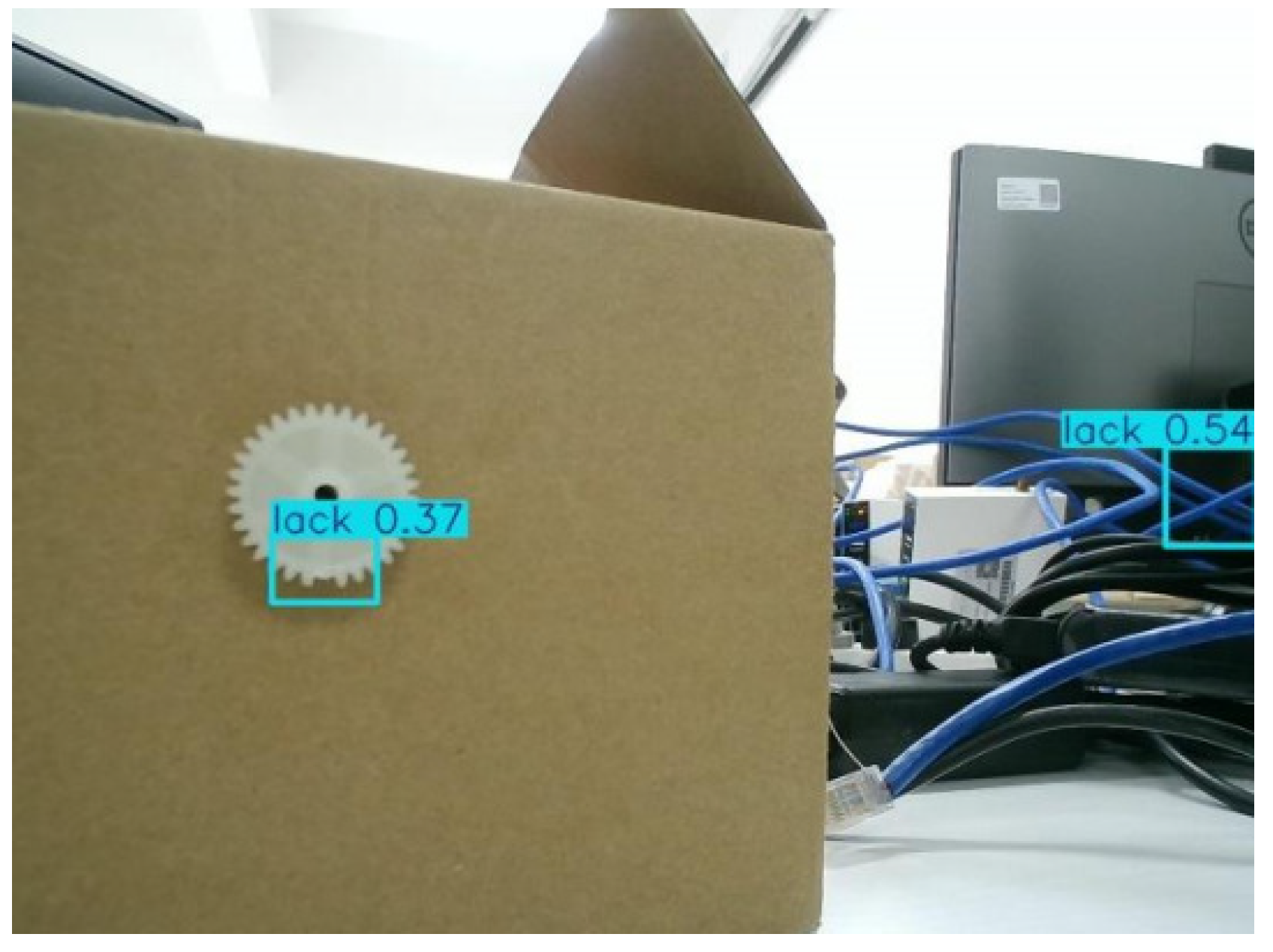
Both frameworks based on hierarchical annotation and training performed well in testing. Under three conditions of imbalance, the G-mean values of both frameworks remained stable at above 0.80, far exceeding the performance achieved when using the public dataset. The poor performance of frameworks trained by the public dataset is due to the significant deviation between the constructed conditions of the public dataset and the actual detection scenarios. The image backgrounds are pure white, lacking the interference information found in complex environments. This results in the features learned during the model training having extremely poor generalization capabilities in real-world tasks. During testing, the system often misidentifies irrelevant factors in the background as faults. For example, as shown in Figure 12, the system mistakenly treats the wires in the background as faults. After using the semi-supervised learning framework, the performance actually decreased. This is due to the lack of two-stage defect area cropping. The system directly extracts features from the collected images, but the gear defect areas in the entire image are very small, resulting in unclear defect features. Features from other areas affect the K-means algorithm, causing the overall performance of the system to decrease. In contrast, the framework based on hierarchical annotation and training demonstrates superior performance. When the imbalance ratio is 2:1:1, the G-mean metric of the semi-supervised learning framework is lower than that of the supervised learning framework. This is because the large number of samples results in closer distances between cluster centers, and the fixed-threshold decision strategy easily leads to the K-means decision covering the CNN prediction, thereby reducing the overall detection accuracy of the system. However, when the imbalance becomes more severe, the G-mean values of the semi-supervised learning framework are all greater than those of the supervised learning framework. This is caused by the fact that the clustering algorithm can classify based on fault features without relying on label information, compensating for the underfitting issue of the deep learning model resulted from the influence of minority class samples. At this point, the fixed threshold setting effectively compensates for the decisions of both approaches. These two phenomena indicate that the threshold in the semi-supervised learning framework should be adaptively set according to specific task requirements.

4. Conclusions

This paper addresses the challenges of tiny target areas and complex backgrounds by proposing a hierarchical annotation training method. The model using the proposed method first crops the entire gear target in a complex environment, then extracts the fault area from the gear target, thereby improving the fault classification capability. To alleviate the sample imbalance issue, a semi-supervised learning framework is introduced based on the extraction of fault areas in the second stage. In this paper, we construct imbalanced datasets using self-shot sample images for model training and deploy it in an actual environment for system testing. The experimental results show that the hierarchical annotation method effectively improves detection accuracy and has certain practical engineering value.
However, there is still room for improvement in our study. The fault areas marked in the second stage are very small, which remains a major challenge for the positioning accuracy of the model. Data augmentation or more powerful deep learning networks will be used in the future research. On the other hand, the threshold setting in semi-supervised models is still flawed and adaptive threshold adjustment is one of the directions for improvement.

Author Contributions

Conceptualization, H.H. and R.W.; methodology, R.W.; software, R.W.; validation, H.H., D.Y., Z.X. and J.W.; formal analysis, D.Y.; investigation, J.W.; resources, R.Z.; data curation, R.W.; writing—original draft preparation, Q.L.; writing—review and editing, H.H. and Q.L.; visualization, J.W.; supervision, Z.X. and D.Y.; project administration, H.H.; funding acquisition, R.Z. All authors have read and agreed to the published version of the manuscript.

Funding

This work was supported by the National Natural Science Foundation of China under Grant 62403136, Innovation Fund Project of Fujian Province Science and Technology Program (2024C0011) and Fujian Province Science and Technology Program (2024H0037).

Data Availability Statement

Dataset available on request from the authors.

Conflicts of Interest

Author Rong Zheng was employed by the company IAP (Fujian) Technology Co., Ltd. The remaining authors declare that the research was conducted in the absence of any commercial or financial relationships that could be construed as a potential conflict of interest.

Abbreviations

The following abbreviations are used in this manuscript:
CNNConvolutional Neural Networks
mAPmean Average Precision
IoUIntersection of Union
G-meanGeometric mean accuracy

References

  1. Lv, H.; Chen, J.; Pan, T.; Zhang, T.; Feng, Y.; Liu, S. Attention mechanism in intelligent fault diagnosis of machinery: A review of technique and application. Measurement 2022, 199, 111594. [Google Scholar] [CrossRef]
  2. Feng, K.; Ji, J.; Ni, Q.; Beer, M. A review of vibration-based gear wear monitoring and prediction techniques. Mech. Syst. Signal Process. 2023, 182, 109605. [Google Scholar] [CrossRef]
  3. Liu, D.; Cui, L.; Wang, H. Rotating Machinery Fault Diagnosis Under Time-Varying Speeds: A Review. IEEE Sens. J. 2023, 23, 29969–29990. [Google Scholar] [CrossRef]
  4. Sharma, V.; Parey, A. A Review of Gear Fault Diagnosis Using Various Condition Indicators. Procedia Eng. 2016, 144, 253–263. [Google Scholar] [CrossRef]
  5. Xiao, J.; Ding, X.; Wang, Y.; Huang, W.; He, Q.; Shao, Y. Gear fault detection via directional enhancement of phononic crystal resonators. Int. J. Mech. Sci. 2024, 278, 109453. [Google Scholar] [CrossRef]
  6. Hashim, S.; Shakya, P. A spectral kurtosis based blind deconvolution approach for spur gear fault diagnosis. ISA Trans. 2023, 142, 492–500. [Google Scholar] [CrossRef] [PubMed]
  7. Junjun, Z.; Quansheng, J.; Yehu, S.; Chenhui, Q.; Fengyu, X.; Qixin, Z. Application of recurrent neural network to mechanical fault diagnosis: A review. J. Mech. Sci. Technol. 2022, 36, 527–542. [Google Scholar] [CrossRef]
  8. Mohammed, O.D.; Rantatalo, M. Gear fault models and dynamics-based modelling for gear fault detection—A review. Eng. Fail. Anal. 2020, 117, 104798. [Google Scholar] [CrossRef]
  9. Dadon, I.; Koren, N.; Klein, R.; Bortman, J. A realistic dynamic model for gear fault diagnosis. Eng. Fail. Anal. 2018, 84, 77–100. [Google Scholar] [CrossRef]
  10. Huang, H.; Peng, X.; Du, W.; Zhong, W. Robust Sparse Gaussian Process Regression for Soft Sensing in Industrial Big Data Under the Outlier Condition. IEEE Trans. Instrum. Meas. 2024, 73, 1–11. [Google Scholar] [CrossRef]
  11. Ahmad, H.; Cheng, W.; Xing, J.; Wang, W.; Du, S.; Li, L.; Zhang, R.; Chen, X.; Lu, J. Deep learning-based fault diagnosis of planetary gearbox: A systematic review. J. Manuf. Syst. 2024, 77, 730–745. [Google Scholar] [CrossRef]
  12. Shao, Z.; Zhang, T.; Kosasih, B. Compound Faults Diagnosis in Wind Turbine Gearbox Based on Deep Learning Methods: A Review. In Proceedings of the 2024 Global Reliability and Prognostics and Health Management Conference (PHM-Beijing), Beijing, China, 11–13 October 2024; pp. 1–8. [Google Scholar]
  13. Sowmya, S.; Saimurugan, M.; Edinbarough, I. Rotational Machine Fault Diagnosis Using Artificial Intelligence (AI) Strategies for the Operational Challenges Under Variable Speed Condition: A Review. IEEE Access 2024, 12, 144870–144889. [Google Scholar] [CrossRef]
  14. Gecgel, O.; Ekwaro-Osire, S.; Dias, J.P.; Serwadda, A.; Alemayehu, F.M.; Nispel, A. Gearbox Fault Diagnostics Using Deep Learning with Simulated Data. In Proceedings of the 2019 IEEE International Conference on Prognostics and Health Management (ICPHM), San Francisco, CA, USA, 17–20 June 2019; pp. 1–8. [Google Scholar]
  15. Heydarzadeh, M.; Kia, S.H.; Nourani, M.; Henao, H.; Capolino, G.A. Gear fault diagnosis using discrete wavelet transform and deep neural networks. In Proceedings of the IECON 2016—42nd Annual Conference of the IEEE Industrial Electronics Society, Florence, Italy, 23–26 October 2016; pp. 1494–1500. [Google Scholar]
  16. Saufi, S.R.; Ahmad, Z.A.B.; Leong, M.S.; Lim, M.H. Gearbox Fault Diagnosis Using a Deep Learning Model with Limited Data Sample. IEEE Trans. Ind. Inform. 2020, 16, 6263–6271. [Google Scholar] [CrossRef]
  17. Krawczyk, B. Learning from imbalanced data: Open challenges and future directions. Prog. Artif. Intell. 2016, 5, 221–232. [Google Scholar] [CrossRef]
  18. Nikpour, B.; Rahmati, F.; Mirzaei, B.; Nezamabadi-pour, H. A comprehensive review on data-level methods for imbalanced data classification. Expert Syst. Appl. 2026, 295, 128920. [Google Scholar] [CrossRef]
  19. Dablain, D.; Krawczyk, B.; Chawla, N.V. DeepSMOTE: Fusing Deep Learning and SMOTE for Imbalanced Data. IEEE Trans. Neural Netw. Learn. Syst. 2023, 34, 6390–6404. [Google Scholar] [CrossRef]
  20. Haixiang, G.; Yijing, L.; Shang, J.; Mingyun, G.; Yuanyue, H.; Bing, G. Learning from class-imbalanced data: Review of methods and applications. Expert Syst. Appl. 2017, 73, 220–239. [Google Scholar] [CrossRef]
  21. Wang, W.; Sun, D. The improved AdaBoost algorithms for imbalanced data classification. Inf. Sci. 2021, 563, 358–374. [Google Scholar] [CrossRef]
  22. Singh, A.; Ranjan, R.K.; Tiwari, A. Credit Card Fraud Detection under Extreme Imbalanced Data: A Comparative Study of Data-level Algorithms. J. Exp. Theor. Artif. Intell. 2022, 34, 571–598. [Google Scholar] [CrossRef]
  23. Ngo, G.; Beard, R.; Chandra, R. Evolutionary bagging for ensemble learning. Neurocomputing 2022, 510, 1–14. [Google Scholar] [CrossRef]
  24. Yang, X.; Song, Z.; King, I.; Xu, Z. A survey on deep semi-supervised learning. IEEE Trans. Knowl. Data Eng. 2022, 35, 8934–8954. [Google Scholar] [CrossRef]
  25. Odena, A. Semi-supervised learning with generative adversarial networks. arXiv 2016, arXiv:1606.01583. [Google Scholar] [CrossRef]
  26. Thekumparampil, K.K.; Wang, C.; Oh, S.; Li, L.J. Attention-based graph neural network for semi-supervised learning. arXiv 2018, arXiv:1803.03735. [Google Scholar]
  27. Rasmus, A.; Berglund, M.; Honkala, M.; Valpola, H.; Raiko, T. Semi-supervised learning with ladder networks. Adv. Neural Inf. Process. Syst. 2015, 28. [Google Scholar]
  28. Lee, D.H. Pseudo-label: The simple and efficient semi-supervised learning method for deep neural networks. In Proceedings of the Workshop on Challenges in Representation Learning, ICML, Atlanta, GA, USA, 20–21 June 2013. [Google Scholar]
  29. Yao, J.; Wang, M.; Mao, X. CDC-YOLO for Gear Defect Detection: Make YOLOv8 Faster and Lighter on RK3588. In Proceedings of the 2024 International Conference on Sensing, Measurement & Data Analytics in the era of Artificial Intelligence (ICSMD), Huangshan, China, 31 October–3 November 2024; pp. 1–6. [Google Scholar]
  30. Ioannou, I.; Christophorou, C.; Nagaradjane, P.; Vassiliou, V. Performance Evaluation of Machine Learning Cluster Metrics for Mobile Network Augmentation. In Proceedings of the 2024 International Conference on Wireless Communications Signal Processing and Networking (WiSPNET), Chennai, India, 21–23 March 2024; pp. 1–7. [Google Scholar]
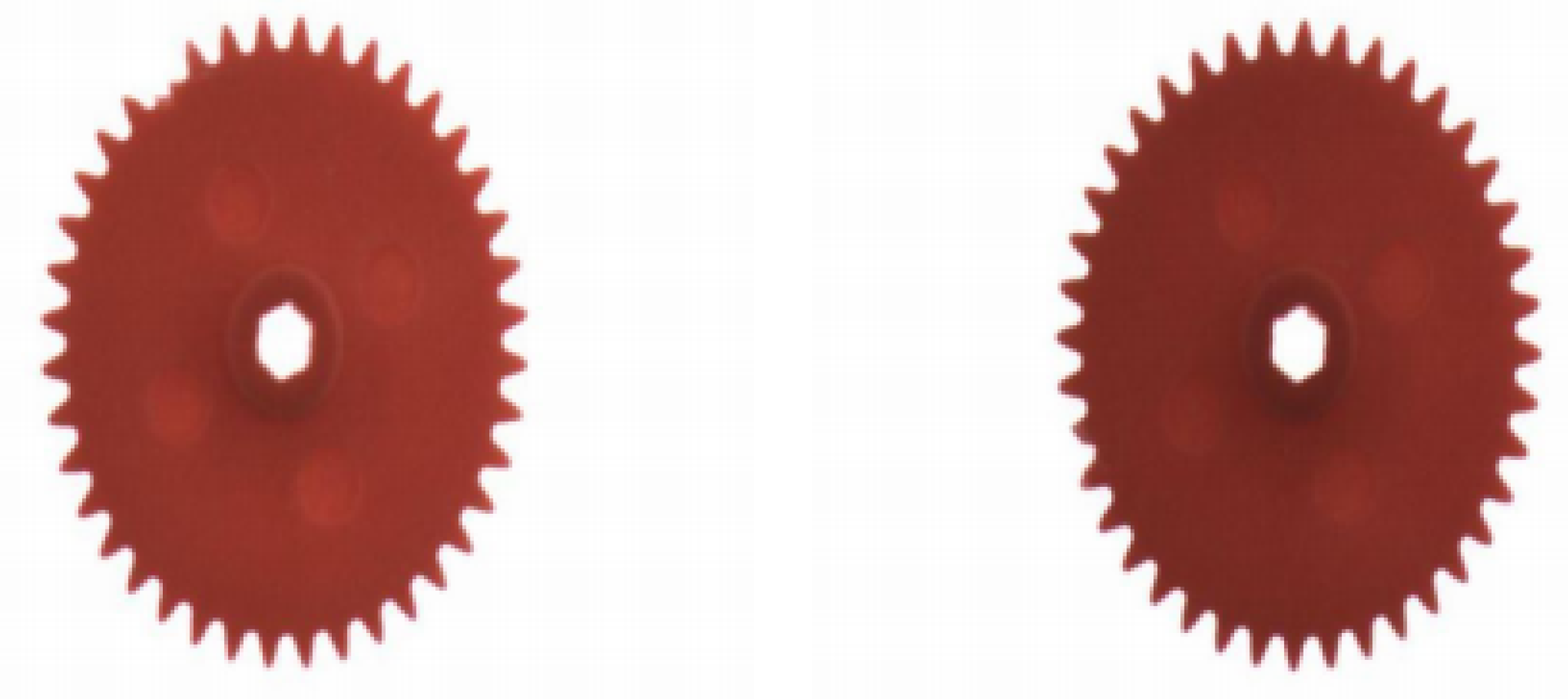
Figure 1. The gear public dataset sample images (https://universe.roboflow.com/gear-u48i0/gear-defect accessed on 24 July 2025). The (left) image shows missing teeth and the (right) shows broken teeth.
Machines 13 00893 g001
Figure 2. Specific dimensions of the hexagonal shaft gear.
Machines 13 00893 g002
Figure 3. Faulty gear sample images.
Machines 13 00893 g003
Figure 4. Examples of images under different shooting conditions. (a) angle = 0°, distance = 40 cm. (b) angle = −15°, distance = 60 cm. (c) angle = 15°, distance = 20 cm.
Machines 13 00893 g004
Figure 5. The overall annotation process and its comparison with traditional methods.
Machines 13 00893 g005
Figure 6. The semi-supervised learning framework.
Machines 13 00893 g006
Figure 7. Panoramic view of the experimental detection platform.
Machines 13 00893 g007
Figure 8. Results of model training in the first stage. The first three columns show the loss during training and validation, and the last two columns show the training metrics.
Machines 13 00893 g008
Figure 9. Training results for the second stage across different epochs. In the first column of the figure, the light-colored points represent actual results, while the solid line corresponds to the smoothed curve.
Machines 13 00893 g009
Figure 10. Confusion matrix heat maps for each model.
Machines 13 00893 g010
Figure 11. Two-dimensional visualization of gear clustering.
Machines 13 00893 g011
Figure 12. One misclassification of the model trained on the public dataset.
Machines 13 00893 g012
Table 1. The parameters of the RMONCAM camera.
ParametersDescriptions
pixel2 million
maximum resolution 1920 × 1080
clarity1080p
communication interfaceUSB
sensor typeCMOS
support systemWindows, Mac OS, Android, Linux
Table 2. The details of the imbalanced datasets.
Degree of ImbalanceNumber of Healthy GearsNumber of Missing GearsNumber of Broken Gears
2:1:1500250250
5:1:1500100100
10:1:15005050
Table 3. The test metrics of each supervised learning model.
Degree of ImbalanceAccuracyTimeCategoryPrecisionRecall
2:1:10.95First stage: 1.17 sHealthy0.93751.0
Second stage: 1.35 sMissing1.00.9143
Total: 2.52 sBroken0.91670.9429
5:1:10.92First stage: 1.16 sHealthy0.85711.0
Second stage: 1.23 sMissing0.97060.9429
Total: 2.39 sBroken0.93550.8286
10:1:10.88First stage: 1.17 sHealthy0.83331.0
Second stage: 1.35 sMissing0.96770.8571
Total: 2.52 sBroken0.84850.80
Table 4. The test metrics of each semi-supervised learning model.
Degree of ImbalanceAccuracyTimeCategoryPrecisionRecall
2:1:10.94First stage: 1.21 sHealthy0.88241.0
Second stage: 1.33 sMissing1.00.9429
Total: 2.54 sBroken0.93940.8857
5:1:10.94First stage: 1.16 sHealthy0.88241.0
Second stage: 1.24 sMissing0.97140.9714
Total: 2.40 sBroken0.96770.8571
10:1:10.90First stage: 1.11 sHealthy0.85711.0
Second stage: 1.19 sMissing0.96880.8857
Total: 2.30 sBroken0.87880.8286
Table 5. The G-mean values of models trained on different datasets.
DatasetsImbalance RatioFrameworks
SupervisedSemi-Supervised
Public1:1:10.1550.035
Self-constructed2:1:10.9280.914
5:1:10.8840.912
10:1:10.8280.857
The bold texts indicate which framework performs better under different degrees of imbalance.
Disclaimer/Publisher’s Note: The statements, opinions and data contained in all publications are solely those of the individual author(s) and contributor(s) and not of MDPI and/or the editor(s). MDPI and/or the editor(s) disclaim responsibility for any injury to people or property resulting from any ideas, methods, instructions or products referred to in the content.