Article

Multi-Objective Structural Parameter Optimization for Stewart Platform via NSGA-III and Kolmogorov–Arnold Network

1
School of Mechanical Science and Engineering, Huazhong University of Science and Technology, Wuhan 430074, China
2
Huazhong Institute of Electro-Optics–Wuhan National Laboratory for Optoelectronics, Wuhan 430223, China
*
Author to whom correspondence should be addressed.
Machines 2025, 13(10), 887; https://doi.org/10.3390/machines13100887
Submission received: 21 August 2025 / Revised: 25 September 2025 / Accepted: 26 September 2025 / Published: 26 September 2025
(This article belongs to the Section Machine Design and Theory)

Abstract

The structural parameters of Stewart platforms play a critical role in enhancing dynamic performance, improving motion accuracy, and enabling effective control strategies. However, practical applications face several key limitations, including the metric balancing for optimization, the limited singularity-free workspace, and low computational efficiency. To overcome those shortcomings, this work proposes a multi-objective optimal design of the structural parameters for Stewart platform based on Non-dominated Sorting Genetic Algorithm III (NSGA-III) and Kolmogorov–Arnold Network (KAN). Firstly, under the stroke constraints of the Stewart platform, this work focuses on optimizing the platform’s key structural parameters. This approach enables both the optimization of existing equipment and the design of new devices. Secondly, this work employs KAN to establish a model that characterizes the relationship between the structural parameters and diverse postures within the maximum singularity-free workspace. This approach not only enhances computational efficiency but also ensures high precision. Finally, this study proposes six performance metrics and utilizes NSGA-III to optimize the structural parameters, thereby achieving a trade-off among these diverse objectives. Simulation and experimental results demonstrate that KAN significantly outperforms the Multi-Layer Perceptron (MLP) in predicting workspace postures. Compared with MLP, KAN achieves higher prediction accuracy and lower error rates across both training and test datasets. When comparing NSGA-III with NSGA-II, the proposed approach demonstrates modest improvements in most performance metrics while preserving acceptable trade-offs between the optimization objectives.

1. Introduction

The Stewart platform, a parallel-kinematic mechanism known for high-precision motion control and strong load-bearing capacity, has been widely used in aerospace engineering [1], precision instrument testing [2], marine wave compensation systems [3], and underwater-vehicle-manipulator-simulation platforms [4]. Given the extensive applications of the Stewart platform, optimizing the structural parameters of this mechanism is of critical importance. This optimization approach maximizes the workspace volume, enhances motion accuracy and dynamic stability, and improves the energy efficiency of the Stewart platform.
Numerous performance indices have been defined to meet these requirements and are applicable to optimization problems [5,6]. Those performance indices include the condition number of the Jacobian matrix [7], velocity amplification factors, and regular workspace shapes as discussed in [8], and the singularity-free workspace [9]. Additionally, stiffness [10], restoration accuracy [11], and the maximum allowable dynamic wrench capability [12] have also been taken into account. Liu [13] employed the condition number and determinant of the kinematic Jacobian matrix as objective functions in the optimal design process. Zhu et al. [14] aimed to achieve the highest positioning accuracy during the design process to determine the optimal geometric parameters of the Stewart platform.
In the past, several optimization methods were proposed for mechanism synthesis, namely the analytical method, single-objective optimization algorithms, and multi-objective optimization algorithms. Some of those methods utilized the analytical form of the objective function to implement the gradient descent method [15]. Nevertheless, when the objective function had no closed-form expression, numerical and evolutionary algorithms were widely used.
Single-objective optimization algorithms are designed to find the optimal solution that either maximizes or minimizes a single objective function. Those algorithms typically operate by iteratively exploring the solution space. Beginning with an initial set of candidate solutions, those algorithms employ specific operators to generate new solutions in each iteration. Differential Evolution (DE) [16,17] and Genetic Algorithms (GA) [18] are two well-known representatives in the domain of single-objective optimization algorithms. Nevertheless, in complex search spaces, both DE and GA frequently encounter premature convergence, becoming prematurely entrapped in local optima. DE and GA exhibit relatively slow convergent speeds, accompanied by limitations in effectively handling multi-modal functions. Li et al. [19] assigned weight coefficients to individual objectives and applied the genetic algorithm to centralize and minimize the natural frequencies of the Hexapod Vibration Isolation System (HVIS). Nevertheless, the use of weight coefficients proved less suitable in this specific case, as weight coefficients were inherently subjective and often difficult to determine with precision. The Artificial Bee Colony (ABC) algorithm [20] was also applied to minimize the weight of structures while satisfying all design requirements. Saputra et al. [21], Wang et al. [22], Duyun et al. [23], and Pisarenko et al. [24] all applied the Particle Swarm Optimization (PSO) algorithm to optimize parameters or determine the workspace of Stewart platform. Nevertheless, the methods [20,21,22,23,24] suffered from low computational efficiency and were incapable of solving multi-objective optimization problems. The Active Set Algorithm [25], Sequential Quadratic Programming (SQP) Algorithm [26], and Interior Point Algorithm [27] were also applied. Nevertheless, those methods were designed for single-objective problems, excelling in single-objective optimization while having limitations in multi-objective scenarios.
Moreover, multi-objective optimization methods, which are designed to optimize multiple conflicting objectives concurrently, have also been employed. Those methods handle complex systems in which enhancing one objective may undermine others, aiming to find a set of Pareto-optimal solutions that represent optimal trade-offs. The Non-dominated Sorting Genetic Algorithm (NSGA-II) [28,29,30,31,32] was used for Multi Objective Optimization (MOO), in which the theory of genetic evolution had been implemented. Nevertheless, when the number of objectives exceeded three in multi-objective optimization, the performance of NSGA-II deteriorated markedly. Another implemented evolutionary algorithm was the Multi-Objective Evolutionary Algorithm based on Decomposition (MOEA/D) [33], which was claimed to be superior to NSGA-II. Nevertheless, the MOEA/D algorithm exhibits high computational complexity, with its efficiency significantly influenced by the population size. Furthermore, only an approximate value for the initial population size required to achieve global search convergence was obtainable. As for NSGA-III [34], this algorithm followed the framework of NSGA-II and outperformed NSGA-II and even MOEA/D in solving many-objective problems. NSGA-III employed reference points and was capable of solving multi-objective optimization problems with a significant number of objective functions.
To address those deficiencies and efficiently optimize structural parameters, while ensuring applicability to any geometric configuration and multiple performance metrics, this work proposes a multi-objective optimal design of the structural parameters in the Stewart platform based on NSGA-III and Kolmogorov–Arnold Network. Firstly, this work mainly focuses on optimizing five key structural parameters within the maximum stroke. This research is applicable to practical applications and can improve the performance indicators of the Stewart platform. Secondly, this work employs NSGA-III to balance multiple performance metrics, including the structural compactness, the force transmission efficiency, the isotropy, the singularity resistance, and orientational workspace capability and positional workspace capability. Thirdly, this work employs a Kolmogorov–Arnold Network [35] to model each orientation and position within the maximum singularity-free workspace. This network exhibits higher fitting accuracy compared with the traditional MLP and is well-suited for real-time computation. The contributions and novelties of this work are presented as follows.
  • This work optimizes five key structural parameters within the maximum stroke. Compared with previous methods, the proposed approach demonstrates superior applicability to practical engineering scenarios and achieves significant improvements in critical performance metrics.
  • This work employs NSGA-III to balance a large number of performance indicators. Compared with previous methods, the proposed approach can take more performance metrics into account and achieve better results.
  • This work employs a Kolmogorov–Arnold Network to model each orientation and position within the maximum singularity-free workspace. Compared with previous methods, this network exhibits higher fitting accuracy than the traditional MLP and is well-suited for real-time computation.
The structure of this paper is presented as follows: Section 2 presents the overview of the proposed method. Section 3 introduces the mathematical model of the Stewart platform, along with the optimization constraint and the optimization indicators. Section 4 delves into the optimization process of the structural parameters of the Stewart platform. Section 5 presents simulations and experiments to validate the optimization effect of the method. Section 6 discusses the results and implications. Finally, Section 7 concludes the study with a summary.

2. Overview

Aiming to optimize the Stewart platform’s structural parameters, this work proposes an algorithm incorporating key performance metrics: the structural compactness, the force transmission efficiency, the isotropy, the singularity resistance, and orientational workspace capability and positional workspace capability. The overview of the proposed method is shown in Figure 1, and the detailed steps are elaborated as follows. This visualization explicitly illustrates the data flow in a sequential process: structural parameters are first input into KAN for workspace metric prediction, then forwarded to NSGA-III for optimization, and finally leading to the derivation of optimal results.
  • Optimizes five key structural parameters of the Stewart platform, a critical kinematic system, under the platform’s stroke constraints. Unlike traditional methods that require comprehensive optimization of numerous parameters, our approach targets five primary parameters to enhance key performance metrics in Stewart platforms. This targeted strategy balances efficiency and precision, avoiding the complexity of adjusting excessive parameters while ensuring systematic performance improvement.
  • Utilizes the KAN, a mathematically proven neural network, for efficient function approximation in the optimization framework. Notably, this approach has the advantage of reducing the computational complexity in genetic algorithms by leveraging a mathematically proven capability to represent any continuous function with minimal layers. Compared to MLPs, KAN outperforms conventional neural networks in both interpretability and approximation accuracy, which makes the KAN particularly suitable for real-time kinematic modeling.
  • Optimize the structural parameters of the Stewart platform using NSGA-III. In contrast to NSGA-II, NSGA-III demonstrates superior performance in addressing multiple conflicting objectives, characterized by uniform solution distribution across the Pareto front, accelerated convergence to optimal regions, and enhanced scalability in high-dimensional objective spaces.

3. Mathematical Modeling for Stewart Platform Optimization

3.1. Structural and Kinematic Characteristics of the Stewart Platform

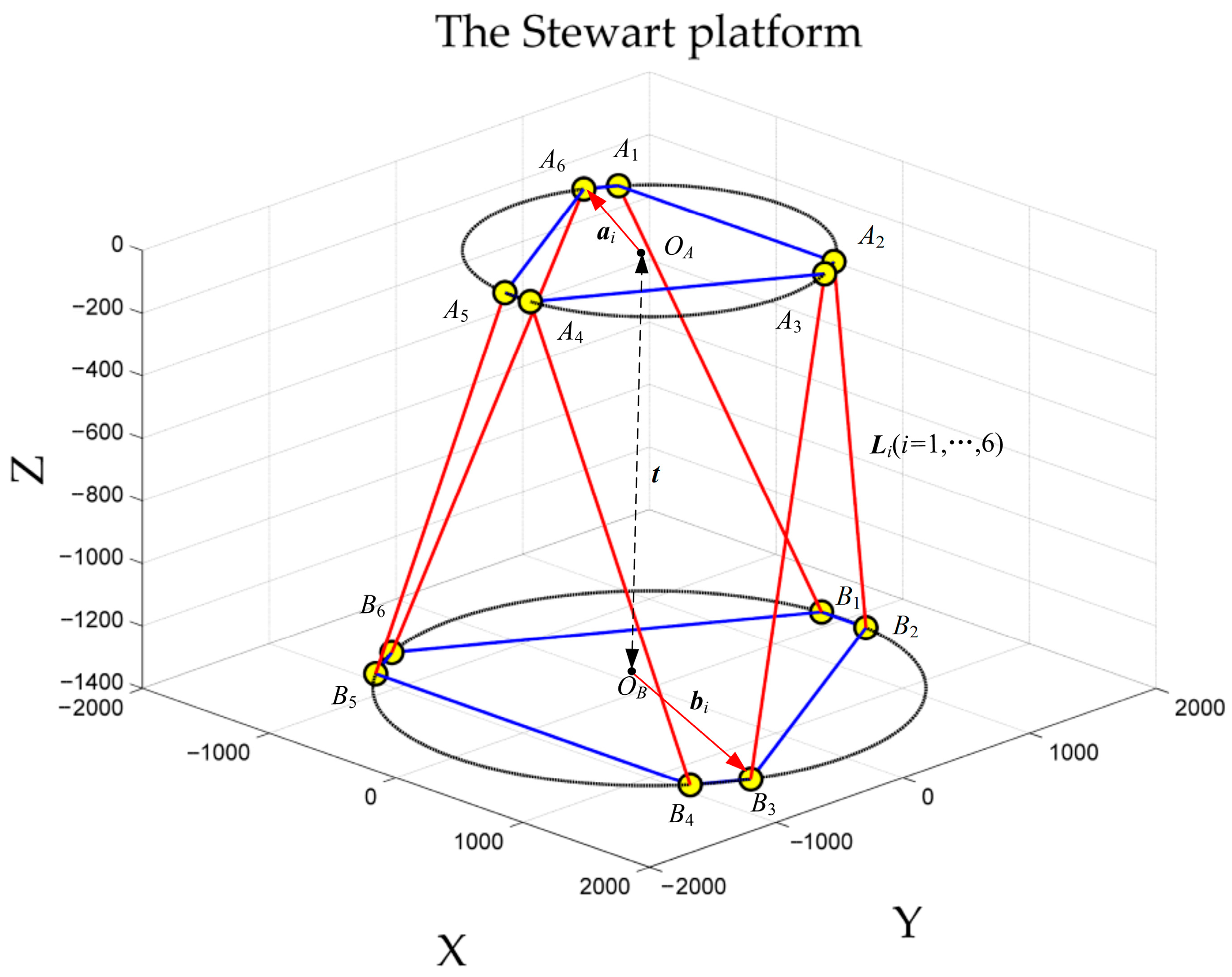
The Stewart platform studied herein is a symmetric 6-DOF parallel robot with universal joints. As analyzed in LAO [36], these universal joints are distributed in equilateral triangles on the upper and lower platforms. As illustrated in Figure 2, it features five key structural parameters: the radii of the moving and fixed platforms R a and R b , the angles θ a and θ b , and the distance d between the circle centers in the initial assembly configuration. These five parameters are the focus of optimization in this study. Such symmetry is widely adopted in engineering because it reduces manufacturing errors and ensures balanced load distribution among the six legs. Figure 2 also labels the translational displacements of the moving platform’s center ( x , y , z ) and the rotational angles determining its orientation ( α , β , γ ), all of which are clearly marked.
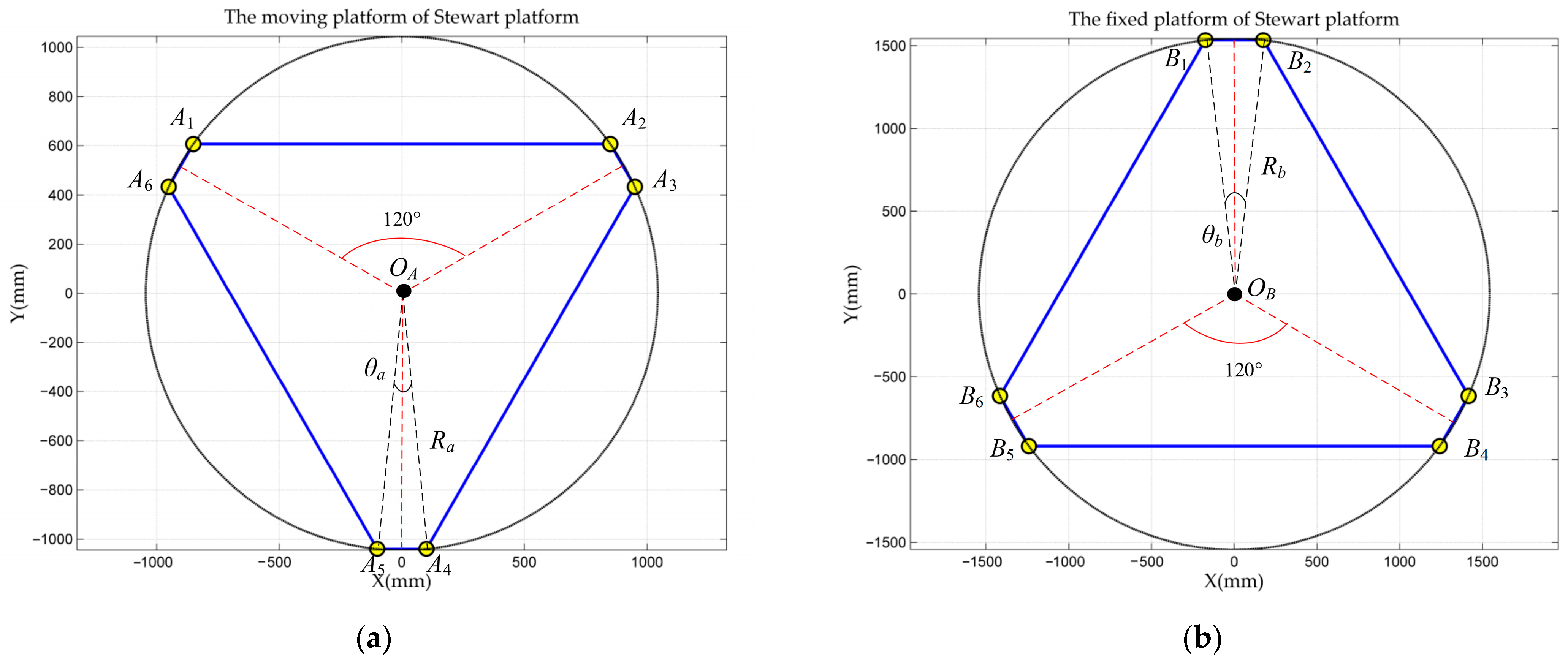
The parameters associated with the moving platform and the fixed platform are presented in Figure 3.
As shown in Figure 3, the joint points of the moving platform ( A 1 A 6 ) and fixed platform ( B 1 B 6 ) are, respectively, distributed on two concentric circles with radii R a and R b ; the figure also labels the central angles θ a (between adjacent A i ) and θ b (between adjacent B i ). The coordinates of joint points on the moving platform are specified as follows:
A =   R a s i n π 3 θ a 2 R a s i n π 3 θ a 2 R a c o s π 6 θ a 2 R a sin θ a 2 R a sin θ a 2 R a cos π 6 θ a 2 R a c o s π 3 θ a 2 R a c o s π 3 θ a 2 R a s i n π 6 θ a 2 R a cos θ a 2 R a cos θ a 2 R a sin π 6 θ a 2 0 0 0 0 0 0
The coordinates of joint points on the fixed platform are specified as follows:
B =   R b sin θ b 2 R b sin θ b 2 R b c o s π 6 θ b 2 R b s i n π 3 θ b 2 R b s i n π 3 θ b 2 R b c o s π 6 θ b 2 R b cos θ b 2 R b cos θ b 2 R b s i n π 6 θ b 2 R b c o s π 3 θ b 2 R b c o s π 3 θ b 2 R b s i n π 6 θ b 2 d d d d d d
The inverse kinematics problem involves calculating the actuator lengths based on the moving platform’s given pose Q , which is defined as follows: Let α (roll, rotation around the x-axis), β (pitch, rotation around the y-axis), and γ (yaw, rotation around the z-axis) denote the rotational angles relative to the Cartesian coordinate system’s three axes; additionally, let x (surge), y (sway), and z (heave) denote the translational displacements along these respective axes:
Q =   [ α ,   β ,   γ ,   x ,   y , z ] T
R denotes the rotation matrix expressed in the Euler angle representation of pitch–roll–yaw, as detailed below:
R =   cos β cos γ s i n α s i n β c o s γ c o s α s i n γ c o s α s i n β c o s γ + s i n α s i n γ c o s β s i n γ s i n α s i n β s i n γ + c o s α s i n γ c o s α s i n β s i n γ s i n α c o s γ s i n β s i n α c o s β c o s α c o s β
With the reference frame fixed, the coordinates of the joint points on the moving platform are a i and those on the fixed platform are b i ( i = 1, …, 6). Here, t is the translation vector from the origin O b of the fixed platform to the origin O a of the moving platform, describing the position offset of the moving platform’s origin relative to the fixed platform’s origin. Based on this, the vectors L i ( i = 1, …, 6) can thus be expressed as follows:
L i = R A i + t b i ,     i   = 1 , , 6
The magnitude of the actuator vector L i corresponds to the length of the i -th electric actuator, which is the key output of the inverse kinematics solution [37].

3.2. Optimization Constraint on Driving Rod Lengths Within Stroke Limits

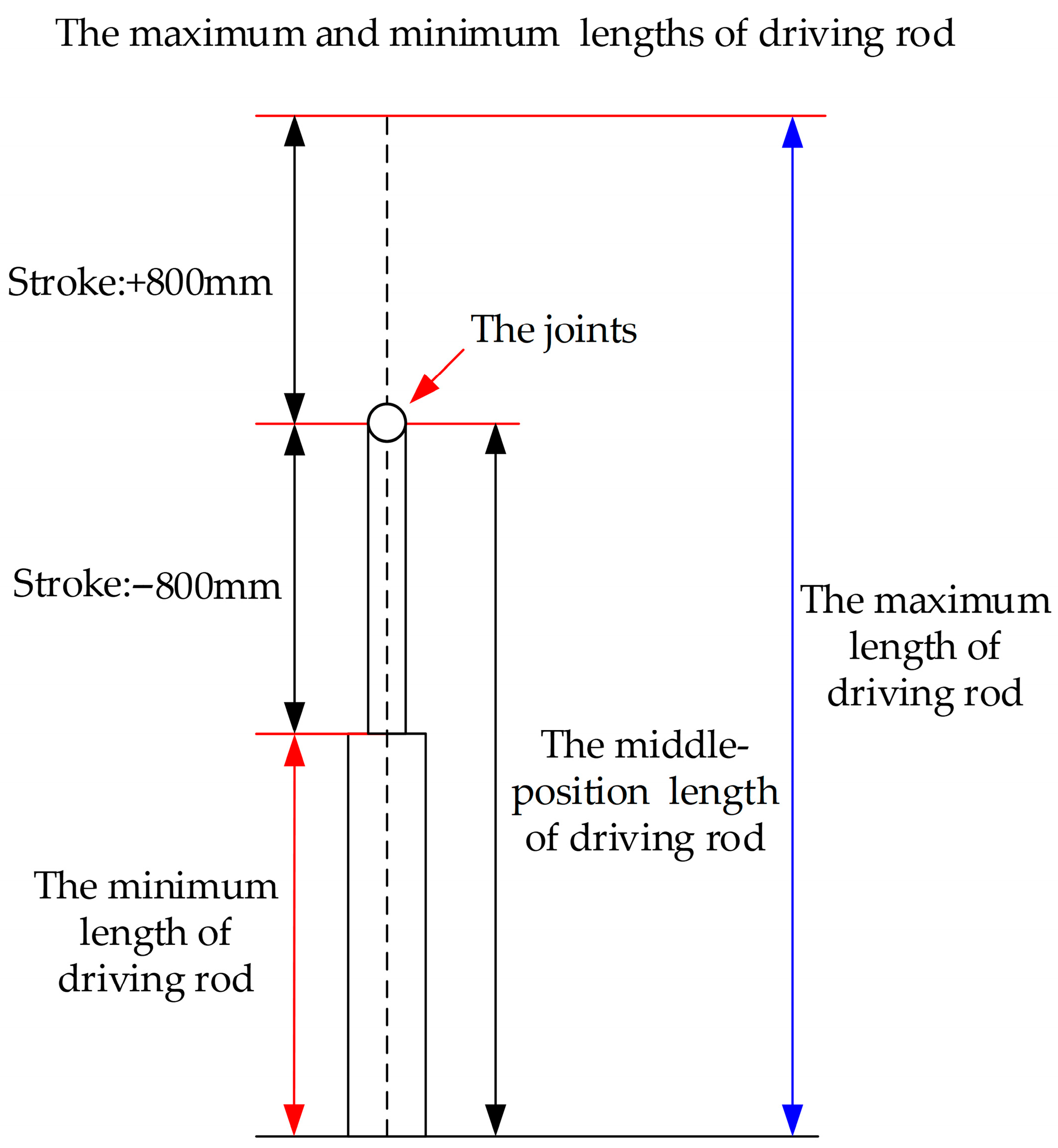
Although the natural lengths of the driving rods connecting the moving and fixed platforms vary, the minimum and maximum strokes of those rods remain invariant. In the multi-objective optimization process, when optimizing the above five parameters, it is necessary to ensure that the stroke of the driving rod stays within a reasonable range—specifically ±800 mm in this paper, as illustrated by the natural-length-based stroke definition in Figure 4. Meanwhile, the length of this variable must ensure no collision among the lengths of all driving rods of the Stewart platform and stay within the maximum and minimum driving strokes.

3.3. Performance Indicators for the Stewart Platform

The Stewart platform in this study is intended for light-load precision manipulation. To address the key requirement of integrating its operational data with structural optimization (outlined in this section), core constraints are defined to delimit the feasible domain for optimization variables ( R a , R b , θ a , θ b , d ). These constraints include two critical aspects: each driving rod’s stroke must stay within practical operational limits to avoid overload; and the moving platform’s positional and attitudinal ranges must align with real-world application requirements, while ensuring these ranges are sufficiently sized to meet operational needs and prevent mechanical interference. The following are several optimization indices for the Stewart platform.
Minimize Structural Compactness ( F 1 )
Optimizing the Stewart platform’s structural parameters to reduce its volume is beneficial. This is particularly true for portable applications, as the optimization enhances portability, reduces material consumption, and may even improve dynamic performance in such scenarios.
This volumetric indicator is calculated as average area multiplied by nominal distance and aligns with “spatial efficiency” in parallel manipulator design, which targets minimizing size for constrained uses (e.g., portable systems), as shown in Ref. [38]. The area of the moving platform is defined in Equation (6):
S A = 3 2 R a 2 ( s i n ( θ a ) + s i n ( 2 π 3 θ a ) )
Meanwhile, the area of the fixed platform is defined in Equation (7):
S B = 3 2 R b 2 ( s i n ( θ b ) + s i n ( 2 π 3 θ b ) )
The structural compactness of the Stewart platform is defined in Equation (8), where F 1 denotes the first optimization indicator and d denotes the nominal distance between the moving and fixed platforms:
F 1 = 1 2 ( S A + S B ) d
This indicator focuses on the spatial occupation of the structure itself for light-load portable scenarios, independent of load weight, applicable to applications with strict volume constraints (e.g., small precision instruments).
Maximize Force Transmission Efficiency ( F 2 )
Performance indicators F 2 , F 3 and F 4 rely on the Stewart platform’s Jacobian matrix J —an 8 × 8 matrix constructed via dual quaternions. The complete form and fundamental derivation of J follow Ref. [37]. This approach aligns with the dual quaternion-based kinematic modeling framework for 6-DOF parallel robots proposed by Yang et al. [39]. Notably, J has inhomogeneous units: one sub-block (for rotational components) is dimensionless, while the other sub-block (for translational components) uses meters. This inhomogeneity is a long-standing challenge in Stewart platform analysis, and Tsai [40] addressed it through dimension-unification strategies. To address this issue, the scaling factor k is adopted from Ref. [37]. Specifically, only the first sub-block of the Jacobian matrix J is scaled by k , while the second sub-block remains unchanged. This relationship is given in Equation (9):
J p =   [ J ζ k , J h ]
where J =   [ J ζ , J h ] denotes the original 8 × 8 Jacobian matrix (constructed with dual quaternions, with J ζ as the first 4 columns and J h as the remaining 4 columns), and J p is the scaled Jacobian matrix. The scaling factor is defined as k   =   t r ( J ζ J ζ T ) t r ( J h J h T ) , and k is defined for the platform’s initial assembly configuration and consequently applies to diverse positions and orientations within the workspace.
This force transmission efficiency indicator reflects the efficiency of energy transfer from the driving rods to the end-effector and is specific to parallel mechanisms. A larger value of this indicator indicates lower energy loss during force transmission, which is critical for precision operations.
D e t ( J p ) represents the determinant of J p . This determinant corresponds to the manipulability concept of a manipulator, first introduced by Yoshikawa [41]. F 2 is defined as the determinant ω of the kinematic Jacobian matrix and serves as the second optimization indicator.
F 2 = ω = d e t ( J p J p T )
Minimize Isotropy ( F 3 )
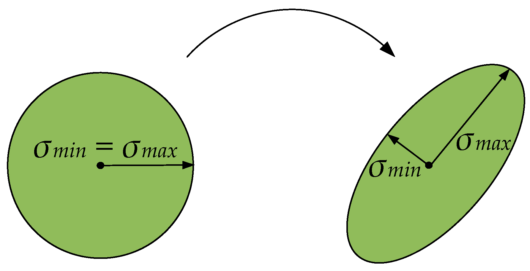
The singular values of the scaled Jacobian matrix J p after unit normalization via the scaling factor k as defined in Equation (4), characterize the “amplification capability” of the matrix across different directions. When the maximum singular value σ m a x and minimum singular value σ m i n are nearly equal (as illustrated by the unit sphere in the left panel of Figure 5), the matrix exhibits isotropic behavior—meaning the platform’s motion and force transmission performance are uniform across all directions. In contrast, a significant disparity between σ m a x and σ m i n (right panel of Figure 5, shown as an ellipse) indicates anisotropy, where performance varies drastically between directions, potentially leading to uneven load distribution or motion limitations [42].
The condition number κ quantifies this anisotropy and is also utilized in Ref. [7] for similar characterization. It is defined as the ratio of the maximum to the minimum of these singular values, as shown in Equation (11):
F 3   =   κ   =   σ m a x σ m i n
A smaller κ (closer to 1) indicates better isotropy, ensuring balanced performance across all degrees of freedom. This is critical for applications requiring uniform precision, such as multi-axis alignment systems.
Maximize Singularity Resistance ( F 4 )
The minimum singular value σ m i n of the Jacobian matrix J p is a key indicator of singularity resistance. This judgment aligns with the research on synthesizing parallel manipulators with singularity-free workspaces [18], where Gallant and Boudreau explicitly verified that σ m i n can directly quantify the distance between a parallel mechanism and its singular configurations.
Specifically, a larger σ m i n means the platform is farther from singular configurations—where σ m i n approaches 0. This distance from singularities brings multiple benefits: it enhances system stability, reduces positional errors, improves robustness in dynamic operations, boosts positional precision, and optimizes manipulator dexterity. Thus, σ m i n acts as the fourth optimization indicator F 4 in Equation (12):
F 4 = σ m i n
Maximize Orientational Workspace Capability ( F 5 )
This indicator quantifies the symmetric rotational range within the singularity-free workspace, with the same filtering applied to exclude singular configurations by preserving the consistent sign of J p ’s determinant.
F 5 = m i n ( m a x α , m i n α , m a x β , m i n β , m a x γ , m i n γ )
where α , β , and γ denote the rotational angles of the moving platform around the global x-axis (roll), y-axis (pitch), and z-axis (yaw), respectively, and are calculated based on Refs. [37,43].
The focus on “symmetric rotational range” aligns with the foundational theory of parallel robot workspace optimization proposed by Gosselin and Angeles [5]. They emphasized that symmetric workspaces enhance operational consistency, which is critical for precision-focused scenarios like small instruments. This design also aligns with the attitudinal range constraints of the moving platform defined in this section, ensuring the calculated rotational workspace is practically feasible. F 5 captures the largest symmetric angular interval for safe rotation, and a larger F 5 indicates a broader symmetric rotational range.
Maximize Positional Workspace Capability ( F 6 )
This indicator quantifies the symmetric translational range within the singularity-free workspace, in which a filtering step is applied to retain only configurations where the sign of the determinant of J p remains unchanged, thus excluding singular positions. The equation is shown as follows:
F 6   =   m i n ( m a x x , m i n x , m a x y , m i n y , m a x z , m i n z )
where x , y , and z denote the translational coordinates of the moving platform’s geometric center in the fixed platform coordinate system.
This coordinate system, whose origin is at the fixed platform’s center and z-axis is perpendicular to the fixed platform’s plane, follows the standard kinematic modeling framework for Stewart platforms. This framework was established in Tsai’s authoritative work on robot analysis [40], ensuring consistency with mainstream design methodologies. These coordinates ( x , y , z ) are calculated with reference to Refs. [37,43]. This coordinate range is constrained by the positional limits of the moving platform specified earlier, aligning the translational workspace with practical operational needs. By taking the minimum of these absolute extrema, the resulting F 6 reflects the largest symmetric interval for safe translation; a larger value of this F 6 thus indicates a broader symmetric translational range.

4. Optimizing the Structural Parameters of the Stewart Platform

4.1. The Multi-Objective Optimization Algorithm NSGA-III

The Non-dominated Sorting Genetic Algorithm (NSGA), a widely used multi-objective optimization algorithm, aims to identify a set of Pareto-optimal solutions within the search space. NSGA classifies solutions into non-dominated fronts according to their non-dominance relationships. Subsequently, genetic operators including selection, crossover, and mutation are employed to iteratively enhance the population, thereby steering the search towards the Pareto-optimal front.
Popular multi-objective evolutionary algorithms NSGA-II and NSGA-III [44] diverge in their diversity maintenance mechanisms: NSGA-II leverages crowding distance for fewer objectives, whereas NSGA-III employs reference-point niching to address ≥3-objective scenarios. Given the six independent optimization metrics detailed in Section 3.3, this study selects NSGA-III for multi-objective parameter optimization due to its demonstrated superiority in high-dimensional objective spaces, a domain where conventional NSGA-II faces scalability limitations.
In this paper, the NSGA-III algorithm is configured with a population size of 100, crossover probability of 0.5, mutation probability of 0.5, and maximum iterations set to 60, and the termination condition is based on reaching the maximum iterations.
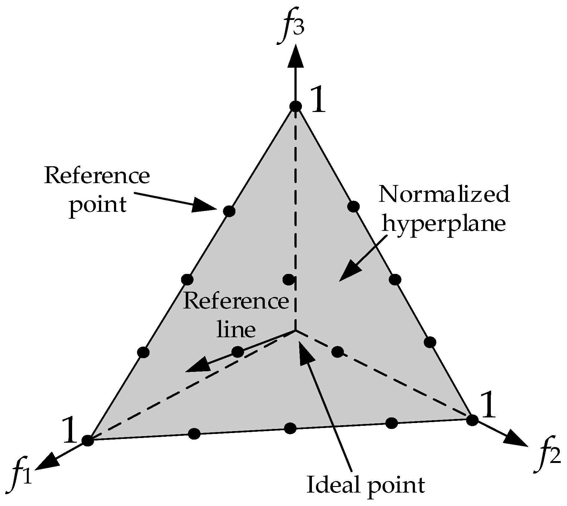
Figure 6 shows 15 reference points on a normalized hyperplane for a three-objective problem ( p = 4). The f 1 , f 2 , f 3 axes (vertex value 1) represent the objectives. The hyperplane is the basic structure, with the ideal point and reference lines aiding in visualizing relationships, facilitating analysis of reference-point distribution for multi-objective optimization.
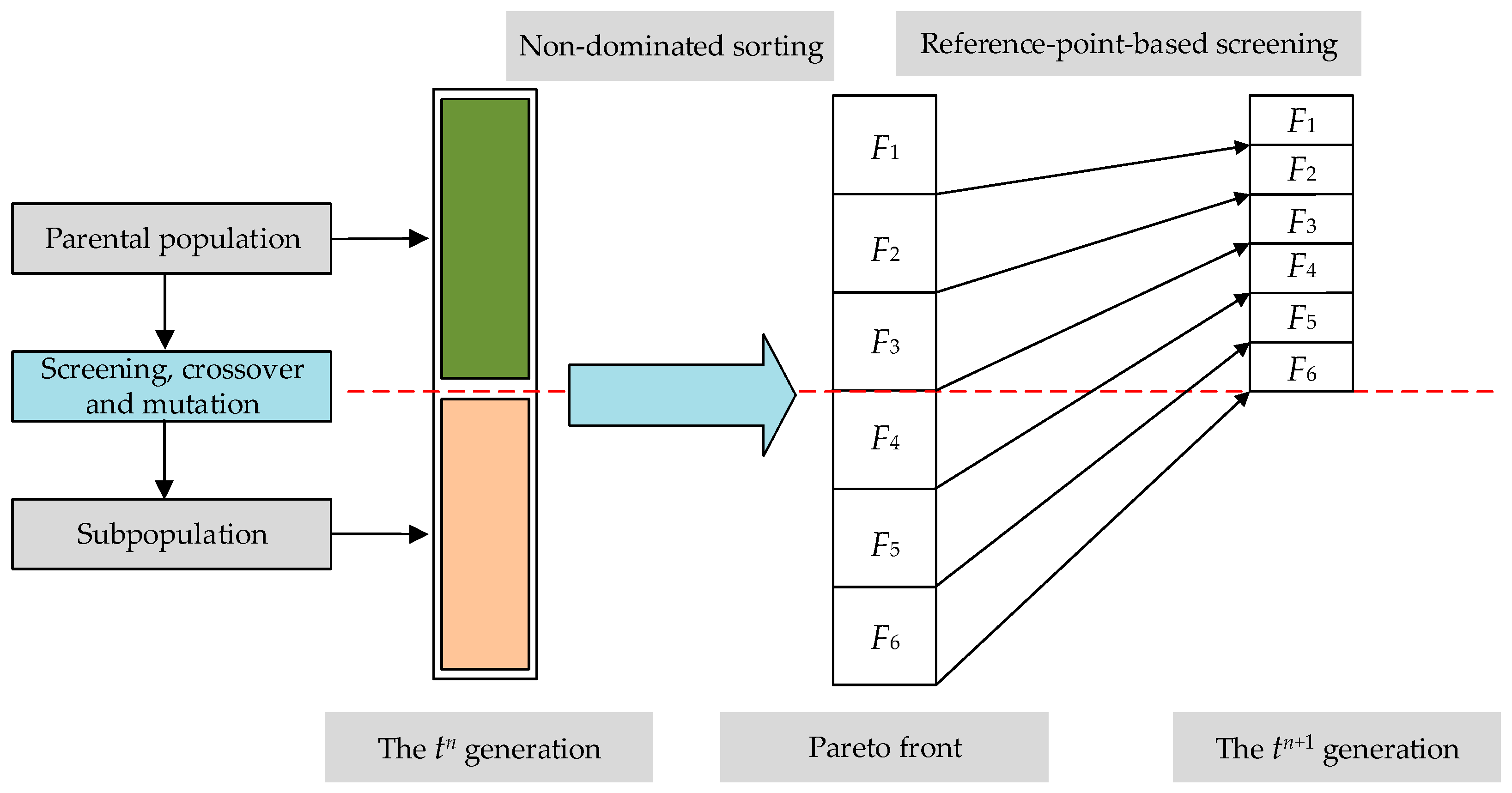
Figure 7 details the evolutionary workflow of the NSGA-III algorithm in multi-objective optimization, elucidating two core mechanisms. First, the parental population (from generation t ) and the subpopulation—produced via selection, crossover, and mutation—are merged into a single candidate set. This merged pool then undergoes non-dominated sorting: solutions are ranked into hierarchical fronts, where a solution A dominates B if A outperforms B in at least one objective and is not inferior in others. In the figure, the upper green region represents the first non-dominated front (the most optimal subset, as no member here is dominated by others), while the lower orange layer contains subsequent dominated fronts.
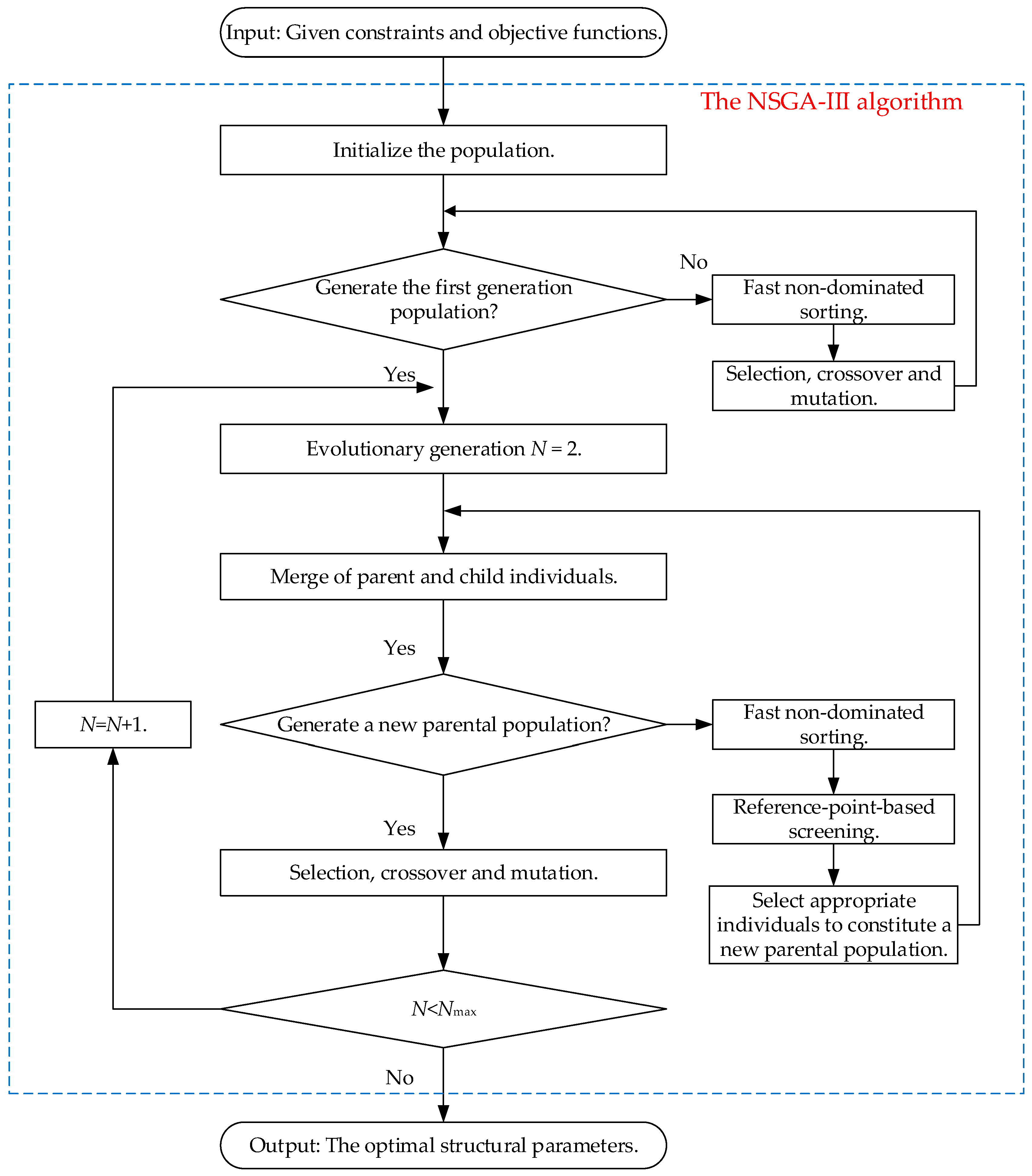
In the NSGA-III algorithm, to eliminate biases caused by disparate objective scales (e.g., varying units or magnitude ranges), each objective function is normalized to the interval [0, 1] using min-max scaling. N represents the current iteration number, while N m a x denotes the predefined maximum iteration number that acts as the termination criterion. This preprocessing ensures equitable participation of all objectives in the optimization process. Figure 8 presents the algorithm’s flowchart, which structures its iterative cycle: starting with population initialization, the workflow involves merging parent and offspring populations, performing non-dominated sorting to identify Pareto-front candidates, and applying reference-point-based screening to preserve solution diversity—highlighting how normalization supports NSGA-III’s core mechanisms for balanced multi-objective parameter optimization. The flowchart of NSGA-III is shown in Figure 8.

4.2. The Neural-Network-Fitting Algorithm KAN

Rooted in Kolmogorov’s theorem, which asserts that any continuous function f : R n R m can be represented as a finite superposition of single-variable functions, KAN instantiates a structured hierarchy of layers designed to enforce this theoretical decomposition. The network architecture comprises three functionally distinct modules: input layer, theorem-specific hidden layers, and output layer [45].
KAN is well-suited for modeling the structural parameter-singularity-free workspace relationship of the Stewart platform due to its edge-based activation aligning with the platform’s kinematic features—strongly nonlinear analytic mappings, high-dimensional sparse parameter interactions, and sharp stroke constraints. Unlike MLP’s node-based activation (which smears information via aggregated nonlinearity), KAN preserves analytic structures, efficiently models sparse couplings, and better adapts to constraints, explaining its superior prediction accuracy, especially near singularity boundaries.
The input layer accepts n -dimensional input vectors corresponding to the structural parameters of the Stewart platform, and the inputs are normalized to the interval [ 1 ,   1 ] via feature-wise min-max scaling to enhance activation function sensitivity and numerical stability. The theorem-specific hidden layers incorporate 2 n + 1 hidden layers required by the theorem for n -dimensional inputs. Those hidden layers are organized into three functional components: phase layers, amplitude layers, and an aggregation layer. The first n layers, termed phase layers, employ trigonometric functions (e.g., sine and cosine) to model periodic dependencies in kinematic mappings. The subsequent n amplitude layers utilize cubic polynomial functions to model the non-linear scaling of input features, complementing the periodic transformations applied by the phase layers. The aggregation layer linearly combines the outputs from the phase and amplitude layers to form a composite representation, adhering to the theorem’s additive superposition principle. Finally, the output layer maps the aggregated hidden representation to the m-dimensional output space. The training protocol balances theoretical and empirical approaches to ensure accurate, physically meaningful solutions for Stewart platform kinematics, involving synthetic dataset generation via forward kinematics, feature normalization, stratified data partitioning, a mean squared error loss with adaptive regularization, and validation through kinematic accuracy metrics and post-training parameter adjustments for generalizability.
The Kolmogorov–Arnold Network (KAN) has emerged as a promising alternative to the Multi-Layer Perceptron (MLP). Both KAN and MLP are underpinned by robust mathematical foundations. Nevertheless, KAN offers greater mathematical rigor, accuracy, and interpretability than MLP. Compared to the standard MLP, KAN makes two main modifications: (1) activation functions change from fixed to learnable components; (2) activation functions are located on edges rather than nodes.
Full Factorial Design was adopted for sampling, involving 5 variables (each divided into 7 intervals) and a total of 16,807 samples. The dataset was split into an 80% training set (13,446 samples) and a 20% validation set (3361 samples). The MLP is a 4-layer network, consisting of 5 input neurons, 2 hidden layers (5 neurons each, with tanh activation), and 6 output neurons. It uses the Adam optimizer (learning rate = 0.001) and MSE as the loss function. The KAN has a width configuration of [5, 5, 5, 6], corresponding to a 4-layer structure (matching the MLP in total neuron count). Its hidden layers use B-spline activation (controlled by grid = 5 and k = 3), with the LBFGS optimizer (1000 training steps) and MSE as the loss function. Both models’ training/test loss curves decline steadily without divergence and show no signs of overfitting.
In terms of activation functions and neuron connections, KAN uses a B-spline activation with “local support” that adjusts outputs only within specific input intervals to capture local nonlinear fluctuations accurately, and it employs adaptive links that dynamically adjust the association strength between neurons, retaining only output-relevant links to avoid redundant noise and focus on core nonlinear relationships for high-precision variables, while MLP relies on a tanh activation that prioritizes global smoothness, struggles with strong local nonlinearity and causes larger local errors, and uses a fixed-weight fully connected structure that introduces redundant associations, weakens the contribution of key features and limits fitting precision.
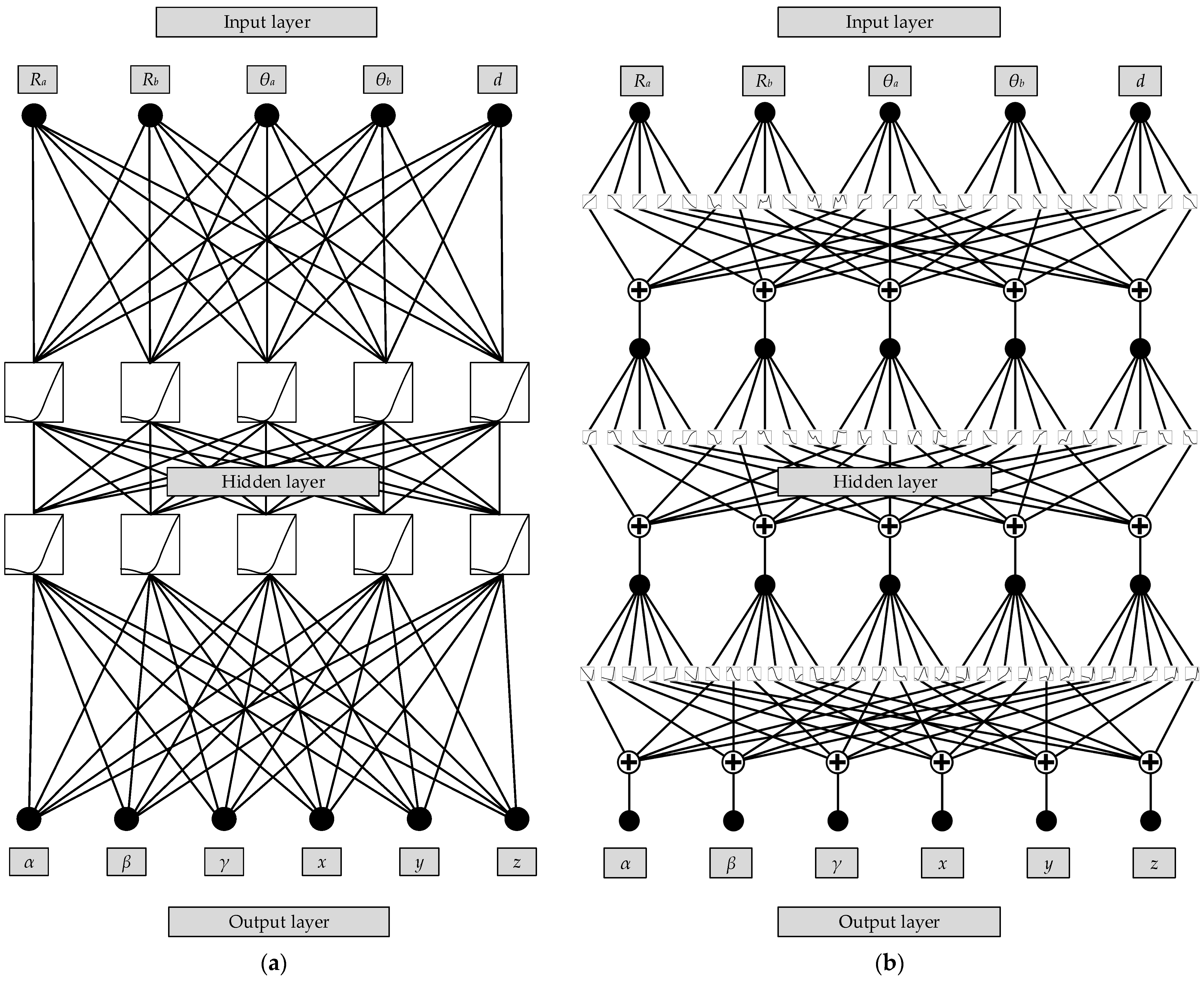
The model architecture designed based on the KAN superposition theorem transforms the approximation and fitting of high-dimensional functions into the learning of one-dimensional variational activation functions with polynomial-level growth. This effectively exploits the smoothness property of spline activation functions, reducing the non-smoothness in the gradient landscape of the approximation function and enhancing the model’s accuracy in approximating the real data distribution. The schematic diagrams of MLP and KAN are presented in Figure 9.
In an MLP, activation functions are applied to the nodes (neurons). For the j-th neuron, the weighted input z j is calculated as follows:
z j   =   i = 1 n w j i x i + b j
where w j i represents the weight from the i-th input neuron to the j-th neuron, x i is the input value corresponding to the i-th input neuron, and b j is the bias of the j-th neuron.
Commonly used fixed activation functions in MLP include the Sigmoid Function, ReLU Function and tanh Function. After passing through the activation function, the output a j of the j-th neuron is as follows:
a j   =   f z j
where f is one of the aforementioned fixed activation functions.
In a KAN, activation functions are placed on the edges and are learnable. Let the set of input-layer nodes be V i n = v 1 , v 2 , , v n T , and the set of hidden-layer nodes be V h i d = u 1 , u 2 , , u m T . The edge from the input-layer node v i to the hidden-layer node u j is denoted as e i j . For the edge e i j , the traditional weight ω i j is replaced by a univariate function ϕ i j x . Assuming a linear spline function, it can be expressed as follows:
ϕ i j x   =   k = 1 K c i j k B k x i
where B k x is the k-th basis function (e.g., B-spline basis function), and c i j k are the learnable coefficients.
Given an input vector X = x 1 , x 2 , , x n T (where x i is the input value for the i-th input node vi), the input s j to the hidden-layer node u j is:
s j   =   i = 1 n ϕ i j x i = i = 1 n k = 1 K c i j k B k x i
Suppose the weights from the hidden layer to the output layer are θ l j ( l represents the index of the output-layer node), and the activation function of the hidden layer is g . The output y l of the output-layer node l is given by:
y l   =   i = 1 m θ l j g s j + b l
where b l is the bias term of the output-layer node y l .
Within an MLP, nodes known as neurons maintain a fixed state. By contrast, KAN uses adjustable activation functions on edges, which act like weights. This system removes all linear weights entirely: each weight becomes a simple function based on a spline. This minor modification enables KAN to outperform MLP in two critical domains: accuracy and understandability. For tasks like fitting data or solving partial differential equations (PDEs), smaller KAN models often match or beat larger MLP models in accuracy. Both theory and experiments show that KAN improves faster with more data than MLP. When it comes to understanding how the model works, KAN allows clear visual explanations and easy human interaction, making it simpler to use than traditional neural networks.

5. Simulations and Experiments

Offline calculation is conducted on a computer equipped with an i9-13980HX processor, boasting a maximum turbo boost frequency of 5.6 GHz, and featuring 32 GB of RAM. The software platform utilized is MATLAB 2024b.

5.1. Experimental Design and Condition

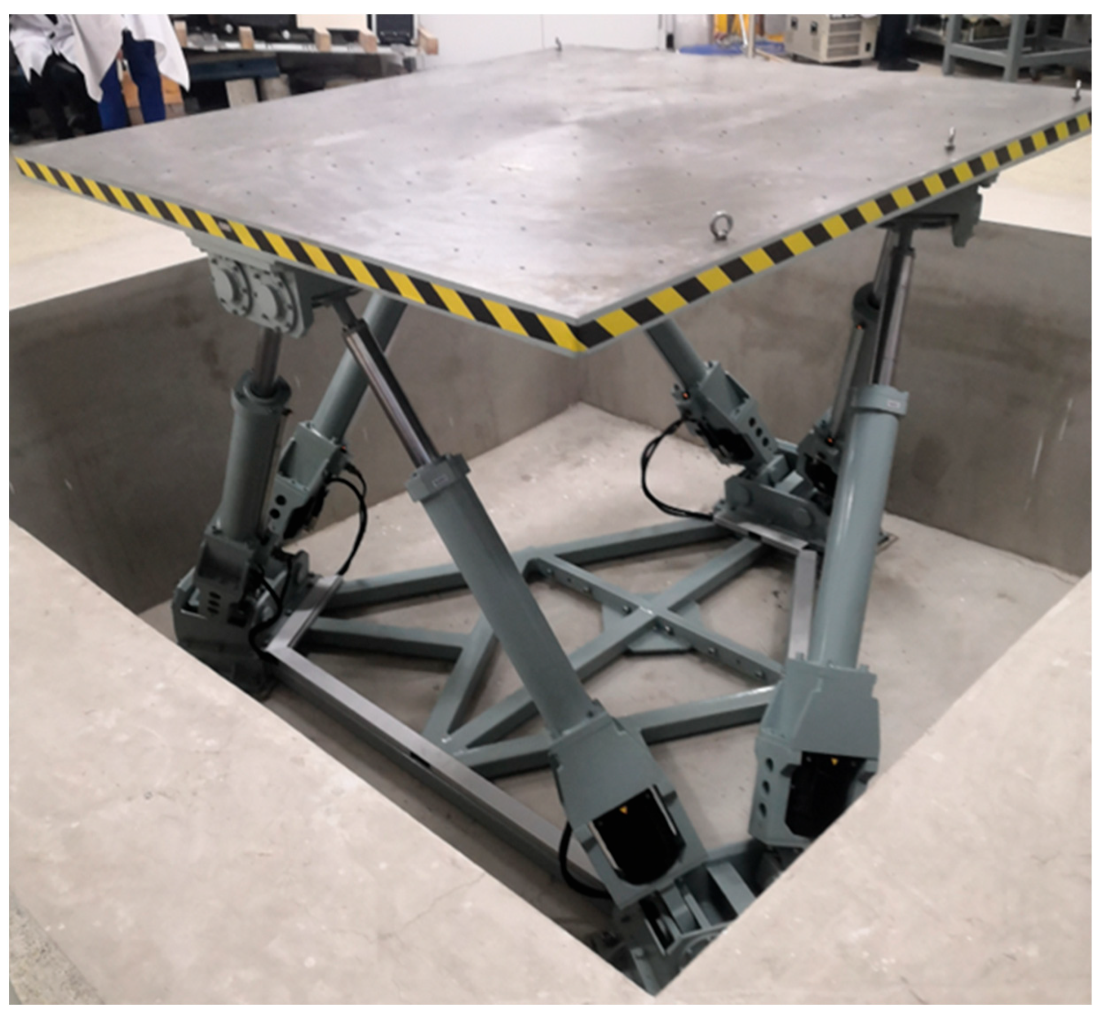
The experimental Stewart platform (YBT6-2000) is shown in Figure 10. For YBT6-2000, R a = 1044.797 mm, R b = 1544.386 mm, θ a = 11°, θ b = 13°, d = 1399.764 mm, and the stroke of the driving rod is ±800 mm. The equipment YBT6-2000 is procured from Wuhan Huazhiyang Technology Co., Ltd., which is situated in Wuhan, China.
For structural parameter optimization, each parameter is adjusted within a defined range around its baseline, with constraints preventing driving rod interference and ensuring rod lengths stay within the Stewart platform’s stroke range. To validly compare KAN and MLP, dataset generation follows a rigorous process: five key system parameters ( R a , R b , θ a , θ b , d ) are randomly sampled within a ±50% range of their default values to reflect practical operational variations, yielding 16,807 unique combinations. All parameter sets are input into Ref. [37]’s kinematic model, incorporating singularity analysis, to generate singularity-free workspace parameters ( α , β , γ , x , y , z ) as training “ground truth”. Training labels derive directly from this theoretical model rather than experiments, eliminating errors and environmental interference to ensure data reliability, and a consistent benchmark for KAN-MLP comparison. The process is shown in Figure 11.
The coordinates of joint points in moving and fixed platforms of YBT6-2000 are shown in Table 1.
The sampling method used is Full Factorial Design, where 5 variables are each divided into 7 equal intervals, resulting in a total of 16,807 samples; the dataset is split into an 80% training set (13,446 samples) and a 20% validation set (3361 samples). For the MLP, it has a 4-layer structure: 5 input neurons, two hidden layers each with 5 neurons, and 6 output neurons. The hidden layers use the tanh activation function, and the model is trained with the Adam optimizer (learning rate = 0.001). For the KAN, its width parameter is set to [5, 5, 5, 6], corresponding to a 4-layer architecture (5 input neurons, two hidden layers each with 5 neurons, and 6 output neurons). It is trained with the LBFGS optimizer for 1000 steps, with additional settings of grid = 5 and k = 3. Both the MLP and KAN show consistent convergence in their training and test loss curves (both curves decline and stabilize without significant divergence), which indicates that the overfitting issue of both models is effectively mitigated.
In neural network training, normalization of input and output data is essential for model convergence and performance. X s c a l e d is the value after normalization, and X is the value before normalization. X m a x and X m i n are the maximum and minimum values, respectively. When normalizing the data to the range between −1 and 1, the formula for normalization is as follows:
X s c a l e d   =   2 ( X X m i n ) X m a x X m i n 1
For different positions and orientations, the following metrics are calculated simultaneously on both the training and validation sets of the neural network, ensuring comprehensive evaluation across all dataset partitions: the coefficient of multiple determination ( R 2 ), mean absolute error (MAE), mean absolute percentage error (MAPE), root mean square error (RMSE), and mean square error (MSE). In Equations (21)–(25), y i (where i = 1, 2, …, n ) represents the actual value in the test set, y ¯ is the average value of y i , and y ^ i denotes the predicted values derived from the neural network:
R 2 = i = 1 n ( y ^ i y ¯ ) 2 i = 1 n ( y i y ¯ ) 2
M A E = 1 n i = 1 n y i y ^ i
M A P E = 1 n i = 1 n y i y ^ i y i × 100 %
M S E = i = 1 n ( y i y ^ i ) 2
R M S E = 1 n i = 1 n ( y i y ^ i ) 2
To evaluate the performance of NSGA-II and NSGA-III on your 6-objective minimization problem, we use one key metric for multi-objective optimization: Spacing (SP). Measures the uniformity of solution distribution. A smaller value indicates more uniform distribution.
Let P = { a 1 ,   a 2 , ,   a n } represent a population of n solutions, where each a i R 6 is a 6-dimensional solution in the objective space. For each solution a i , compute the minimum Euclidean distance to all other solutions in P :
m i = m i n             j i j = 1 , 2 , , n a i a j 2
where . 2 denotes the Euclidean distance in 6-dimensional space.
Mean nearest-neighbor distance is defined as:
ε   = 1 n i = 1 n m i
Spacing (SP) quantifies the uniformity of these distances: a smaller value indicates more evenly distributed solutions.
S P = 1 n 1 i = 1 n ( m i ε ) 2

5.2. Experimental Results and Analysis

As R a varies, the six indicator values F 1 , F 2 , …, F 6 exhibit distinct variations, as visualized in Figure 12. These graphs illustrate the dynamic relationships between each performance indicator and the design parameter R a , while quantitatively demonstrating their parametric evolution and sensitivity trends.
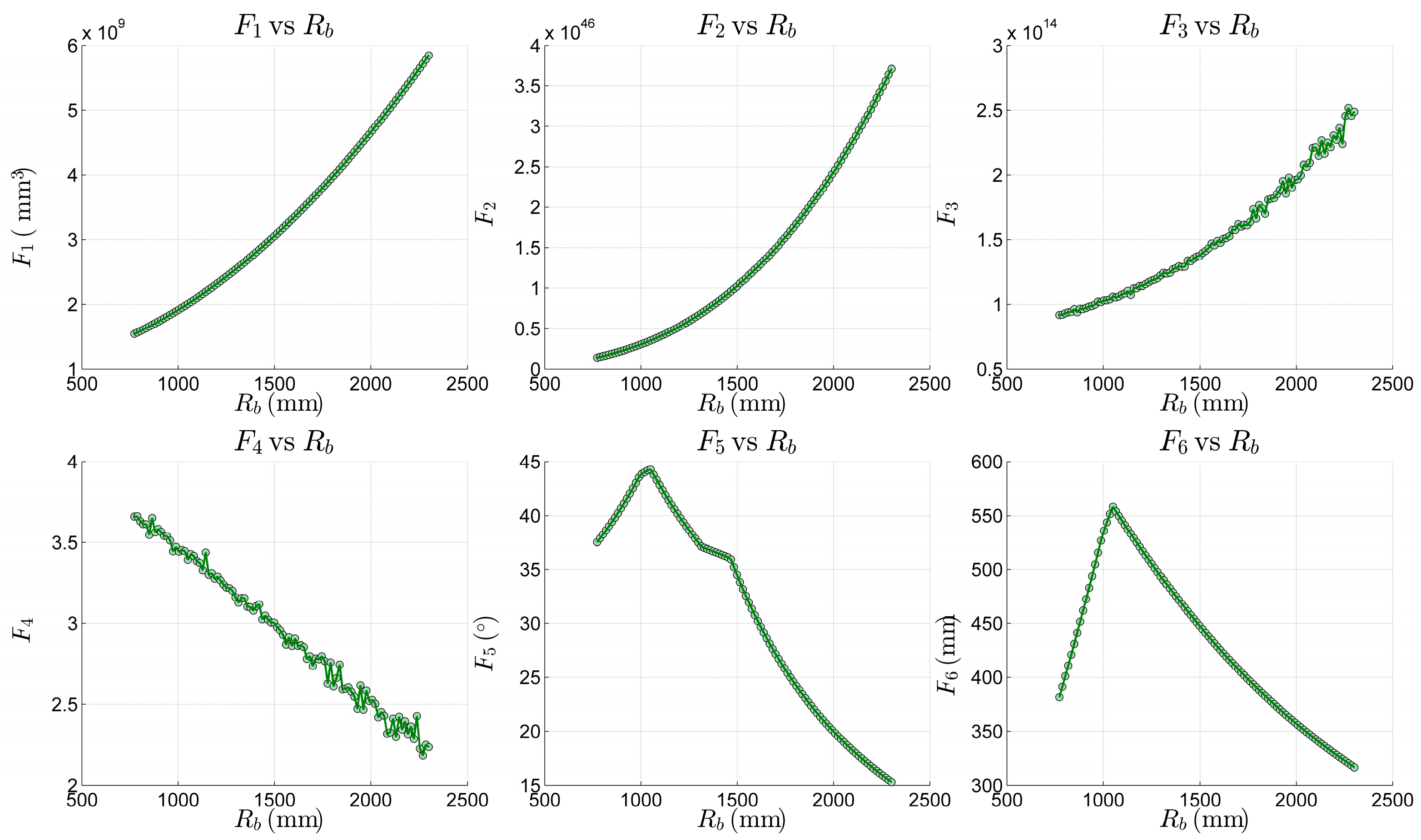
Figure 13 visualizes distinct variations of F 1 F 6 with R b , illustrating their dynamic relationships and sensitivity trends to the design parameter R b .
Figure 14 visualizes distinct variations of F 1 F 6 with θ a .
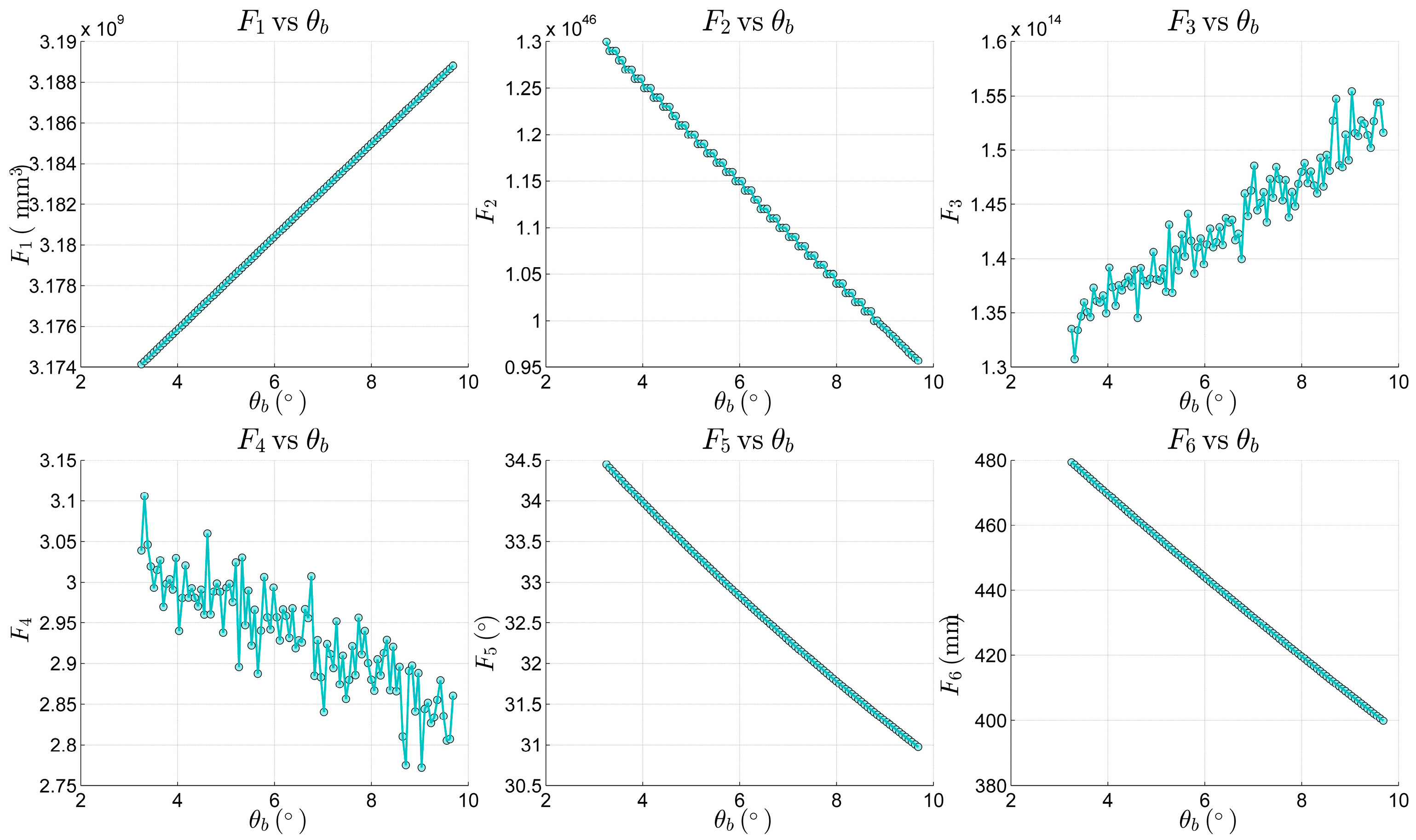
Figure 15 visualizes distinct variations of F 1 F 6 with θ b .
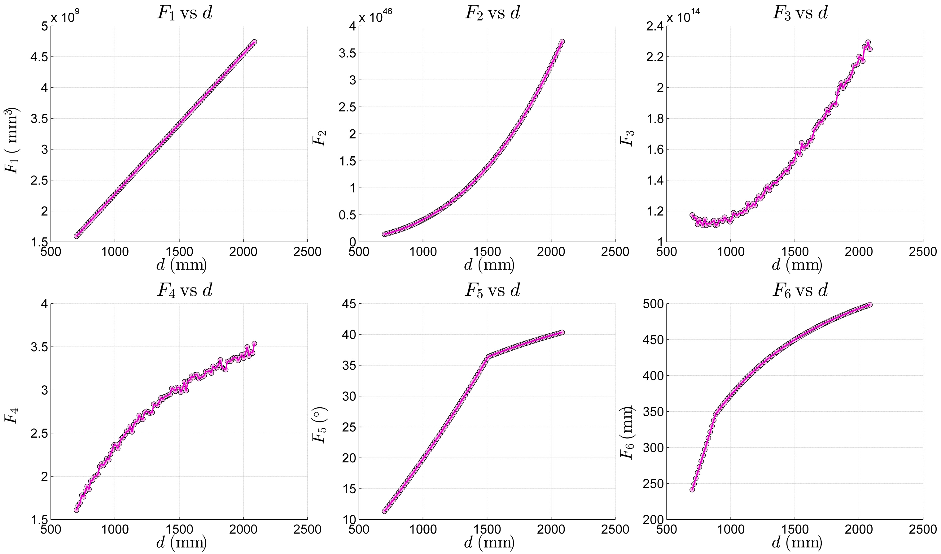
Figure 16 visualizes distinct variations of F 1 F 6 with d .

5.3. Comparison of Efficiency, Accuracy, and Multi-Objective Performance

Both the MLP and KAN neural networks are designed as multi-input multi-output (MIMO) architectures. These networks possess two hidden layers, and each layer contains five neurons. The MLP and KAN neural networks are trained for 1000 epochs, and the comparison of the five metrics is shown below. Table 2 shows that, for the train set, the R 2 of KAN is 3.18% higher than that of MLP. Meanwhile, the MAE, MAPE, MSE, and RMSE of KAN decreased by 85.81%, 87.38%, 97.40%, and 84.53%, respectively, compared with those of MLP.
Table 3 shows that, for the test set, the R 2 of KAN is 3.20% higher than that of MLP. Meanwhile, the MAE, MAPE, MSE, and RMSE of KAN decreased by 85.09%, 81.46%, 97.20%, and 83.54%, respectively, compared with those of MLP.
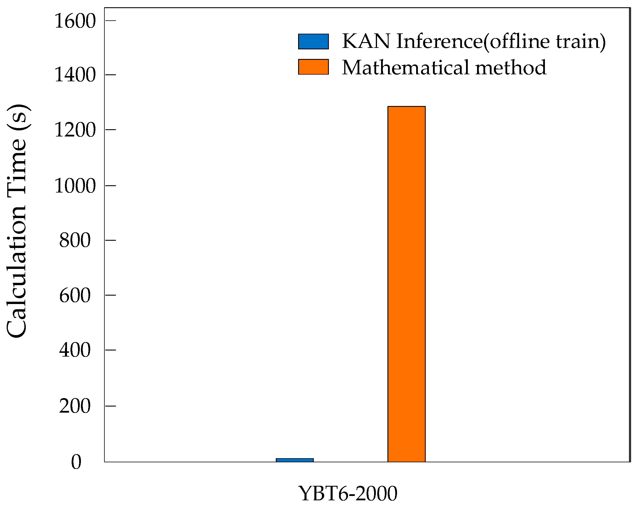
The mathematical method from Ref. [37] takes 1027.43 s for a single maximum singularity-free workspace computation, while the KAN neural network after one 45.07-s training achieves 3.877-millisecond single inference for the same task, showing 99.999% efficiency improvement with consistent single-task comparison. A comparison of the time taken by the two approaches is illustrated in Figure 17.
Under default parameter settings, the structural parameters differ from the values obtained by the NSGA-II and NSGA-III algorithms. Specifically, NSGA-III yields the highest performance index, followed by NSGA-II, with the default configuration achieving the lowest index values. Table 4 presents the structural parameters for the default configuration, NSGA-II, and NSGA-III, with the optimal value of these parameters identified as in NSGA-III.
The NSGA-III Pareto optimal set contains multiple non-dominated solutions, each balancing the six performance metrics. The solution was selected in two steps: first, solutions violating practical engineering constraints were excluded, such as those with parameters beyond equipment’s structural strength or operating range and inapplicable in practice; second, among remaining feasible solutions, the Technique for Order Preference by Similarity to Ideal Solution (TOPSIS) was used to calculate comprehensive scores. Since the six metrics are equally important to the research objectives, each was assigned an equal weight of 1/6. By quantifying each solution’s proximity to the ideal optimal solution, the NSGA-III solution in Table 5 achieved the highest comprehensive score because it balances accuracy, efficiency, and other key dimensions optimally, thus being identified as the final optimal parameter combination. The comparison of the six optimization indicators for the default parameters, NSGA-II, and NSGA-III is presented below.
Compared with the default parameter, NSGA-II shows mixed performance across the six indicators. For F 2 , where larger values are preferable, NSGA-II outperforms the default parameter with a 117.6% increase (from 1.121 × 1046 to 2.439 × 1046). In terms of F 4 F 6 , where larger values are preferable, NSGA-II also demonstrates improvements: F 4 increases by 16.2%, F 5 by 37.5%, and F 6 by 48.7%. However, NSGA-II is inferior in F 1 and F 3 , where smaller values are preferable, with F 1 increasing by 12.6% and F 3 by 13.9% compared to the default parameter.
When comparing NSGA-III with NSGA-II, NSGA-III excels in three key indicators aligned with their optimization directions. For F 1 and F 3 , where smaller values are preferable, NSGA-III achieves significant reductions of 60.9% (from 3.582 × 10⁹ to 1.400 × 10⁹) and 57.1% (from 1.631 × 10¹⁴ to 6.990 × 10¹³), respectively. For F 4 and F 5 , where larger values are preferable, NSGA-III shows marginal improvements of 2.2% and 6.2%, respectively. Conversely, NSGA-III lags in F 2 , where larger values are preferable, with a 94.3% decrease and in F 6 , where larger values are preferable, with a 23.0% decrease compared to NSGA-II.
This performance pattern arises from NSGA-III’s reference-point-based niching strategy, which enhances solution distribution across multi-objective spaces. By systematically guiding solutions toward predefined reference points, NSGA-III effectively balances improvements in indicators requiring smaller values ( F 1 , F 3 ) and those requiring larger values ( F 4 , F 5 ), despite trade-offs in F 2 and F 6 . This balance underscores its superiority in handling the six-dimensional optimization framework, where maintaining diversity across conflicting objectives is critical.
In multi-objective optimization, solution distribution matters. We use the Spacing (SP) metric—smaller values mean more uniform distribution. Table 6 shows SP values for NSGA-II and NSGA-III.
This stems from NSGA-III’s reference-point-based niching strategy, which boosts distribution. Quantitatively, NSGA-III’s smaller SP (0.018 vs. 0.040) confirms more even distribution in the six-dimensional space. This enhances NSGA-III’s fit for high-dimensional, complex multi-objective problems needing diverse, evenly spread solutions.

6. Discussion

This study provides valuable insights into MLP/KAN performance and the effectiveness of optimization algorithms.
For neural networks, KAN outperforms MLP across key metrics. On the training set, KAN achieved 3.18% higher R 2 (superior data fitting) and reduced MAE, MAPE, MSE, RMSE by 85.81–97.40%. On the test set, the gap narrowed, but KAN still maintained 3.20% higher R 2 and 81.46–97.20% lower errors, showing better generalization. It also exhibited strong efficiency, with an average inference time of 3.877 milliseconds—over 99.999% faster than the 1027.43-s single computation time of the mathematical method from Ref. [37]. This efficiency is critical for large datasets or real-time use.
Regarding optimization algorithms, comparisons across six indicators showed: NSGA-II outperformed the default configuration in five ( F 2 , F 4 F 6 ) but lagged in two ( F 1 , F 3 ); NSGA-III improved on four ( F 1 , F 3 , F 4 , F 5 ) but regressed in F 2 / F 6 . This F 2 / F 6 decline stems from intrinsic indicator trade-offs: F 2 / F 6 conflict with F 1 / F 3 , so prioritizing F 1 / F 3 optimization (to meet core needs) inevitably compromises F 2 / F 6 —this is not an algorithmic limitation but indicator mutual exclusivity.
In conclusion, neural network architectures and optimization strategies must align with application needs. KAN stands out for its accuracy, error control, and efficiency, making it robust for complex modeling. For optimization, multi-indicator evaluation is key to matching parameters with engineering goals. Future research could explore KAN-integrated hybrid frameworks and in-depth sensitivity analyses.

7. Conclusions

To address the limitations of existing methods and enable efficient acquisition of optimal structural parameters for diverse geometric and performance requirements, this research introduces a novel framework for optimizing the Stewart platform’s design using NSGA-III and the KAN. Firstly, this work primarily focuses on optimizing the five key structural parameters within the actuator’s maximum stroke range. Secondly, this work applies KAN to fit every orientation and position within the workspace. This network demonstrates higher fitting precision compared to the conventional MLP and is well-adapted for real-time computations. Thirdly, this paper predominantly utilizes NSGA-III to strike a balance among multiple metrics, including the volume, the condition number, the minimum singular value of the Jacobian matrix, the determinant of the Jacobian matrix, and all positions and orientations within the workspace.
When compared with previous algorithms for solving the FKP, the proposed method offers the following advantages: (1) The proposed method conducts an optimal design of the Stewart platform’s structural parameters by taking into account the five key parameters. In traditional methods, the optimization of structural parameters usually occurs during the design stage and involves dealing with all parameters. Nevertheless, practical applications demand optimizing five key parameters to enhance performance characteristics. (2) KAN provides a crucial theoretical foundation for function approximation. It has been proven that a network with a specific structure can approximate any continuous function. Moreover, compared with the MLP, KAN has better interpretability and higher accuracy. (3) This study employs NSGA-III to optimize the Stewart platform’s structural parameters, capitalizing on the algorithm’s capability to manage multiple conflicting objectives. Compared with NSGA-II, NSGA-III demonstrates superior performance through enhanced solution distribution, faster convergence, and greater scalability in high-dimensional search spaces.
Simulations and experiments indicate that for the training set, KAN’s R 2 is 3.18% higher than that of MLP. Meanwhile, KAN achieves reductions of 85.81%, 87.38%, 97.40%, and 84.53% in MAE, MAPE, MSE, and RMSE, respectively, compared with MLP. For the test set, KAN’s R 2 remains 3.20% higher than MLP’s, and it continues to show improvements in error metrics, with MAE, MAPE, MSE, and RMSE decreasing by 85.09%, 81.46%, 97.20%, and 83.54%, respectively, compared with MLP. In terms of NSGA-III, it outperforms NSGA-II in four of the six optimization metrics ( F 1 , F 3 , F 4 , F 5 ), demonstrating significant improvements of 60.9%, 57.1%, 2.2%, and 6.2%, respectively. The F 2 parameter lags with a 94.3% decrease, and the F 6 parameter is 23.0% worse compared to NSGA-II. NSGA-III’s reference-point-based niching strategy enables uniform Pareto front distribution, crucial for balancing conflicting objectives—such as reducing F 1 / F 3 and enhancing F 4 / F 5 —despite trade-offs in F 2 and F 6 . This strategy, evidenced by NSGA-III’s smaller SP value (0.018 vs. 0.040) confirming more even distribution in six-dimensional space, enhances its suitability for high-dimensional, complex multi-objective problems requiring diverse, evenly spread solutions. This highlights the approach’s effectiveness in trade-off optimization under structural constraints, offering quantitative guidance for performance-driven parameter tuning in parallel mechanism designs.

Author Contributions

Conceptualization, methodology, software, validation, formal analysis, resources, data curation, writing—original draft preparation, and visualization by J.T.; investigation, writing—review and editing, supervision, and project administration by H.Z. (Huicheng Zhou); software and validation support by Y.X. and Y.C.; formal analysis and data curation by P.C. and H.Z. (Haikun Zhang); investigation and resources by J.W. All authors have read and agreed to the published version of the manuscript.

Funding

This research was funded by Research on Key Technologies of High-Performance CNC System Product Package (2023BAA010-1).

Data Availability Statement

Data are contained within the article.

Conflicts of Interest

The authors declare no conflicts of interest.

References

  1. Velasco, J.; Calvo, I.; Barambones, O.; Venegas, P.; Napole, C. Experimental Validation of a Sliding Mode Control for a Stewart Platform Used in Aerospace Inspection Applications. Mathematics 2020, 8, 2051. [Google Scholar] [CrossRef]
  2. Liu, Z.; Cai, C.; Yang, M.; Zhang, Y. Testing of a MEMS Dynamic Inclinometer Using the Stewart Platform. Sensors 2019, 19, 4233. [Google Scholar] [CrossRef]
  3. Li, D.; Wang, S.; Song, X.; Zheng, Z.; Tao, W.; Che, J. A BP-Neural-Network-Based PID Control Algorithm of Shipborne Stewart Platform for Wave Compensation. J. Mar. Sci. Eng. 2024, 12, 2160. [Google Scholar] [CrossRef]
  4. Cetin, K.; Tugal, H.; Petillot, Y.; Dunnigan, M.; Newbrook, L.; Erden, M.S. A Robotic Experimental Setup with a Stewart Platform to Emulate Underwater Vehicle Manipulator Systems. Sensors 2022, 22, 5827. [Google Scholar] [CrossRef]
  5. Gosselin, C.; Angeles, J. A global performance index for the kinematic optimization of robotic manipulators. J. Mech. Des. 1991, 113, 220–226. [Google Scholar] [CrossRef]
  6. Chiu, S. Kinematic characterization of manipulators: An approach to defining optimality. In Proceedings of the 1988 IEEE International Conference on Robotics and Automation, Philadelphia, PA, USA, 24–29 April 1988; pp. 828–833. [Google Scholar]
  7. Li, Y.; Yang, X.L.; Wu, H.T.; Chen, B. Optimal Design of a Six-Axis Vibration Isolator via Stewart Platform by Using Homogeneous Jacobian Matrix Formulation Based on Dual Quaternions. J. Mech. Sci. Technol. 2018, 32, 11–19. [Google Scholar] [CrossRef]
  8. Chablat, D.; Wenger, P.; Majou, F.; Merlet, J.-P. A novel method for the design of 2-dof parallel mechanisms for machining applications. Int. J. Robot. Res. 2007, 23, 615–624. [Google Scholar] [CrossRef]
  9. Salunkhe, D.H.; Michel, G.; Kumar, S.; Sanguineti, M.; Chablat, D. An Efficient Combined Local and Global Search Strategy for Optimization of Parallel Kinematic Mechanisms with Joint Limits and Collision Constraints. Mech. Mach. Theory 2022, 173, 104796. [Google Scholar] [CrossRef]
  10. Zhang, T.; Gong, X.; Zhang, L.; Yu, Y. A New Modeling Approach for Parameter Design of Stewart Vibration Isolation System Integrated into Complex Systems. Machines 2022, 10, 1005. [Google Scholar] [CrossRef]
  11. Tu, Y.Q.; Yang, G.L.; Cai, Q.Z.; Wang, L.F.; Zhou, X. Optimal design of SINS’s Stewart platform bumper for restoration accuracy based on genetic algorithm. Mech. Mach. Theory 2018, 124, 42–54. [Google Scholar] [CrossRef]
  12. Lee, C.J.; Chen, C.T. Reconfiguration for the Maximum Dynamic Wrench Capability of a Parallel Robot. Appl. Sci. 2016, 6, 80. [Google Scholar] [CrossRef]
  13. Liu, G. Optimal Kinematic Design of a 6-UCU Kind Gough-Stewart Platform with a Guaranteed Given Accuracy. Robotics 2008, 7, 30. [Google Scholar] [CrossRef]
  14. Zhu, M.; Huang, C.; Song, S.; Gong, D. Design of a Gough–Stewart Platform Based on Visual Servoing Controller. Sensors 2022, 22, 2523. [Google Scholar] [CrossRef] [PubMed]
  15. Germain, C.; Caro, S.; Briot, S.; Wenger, P. Optimal design of the IRSBot-2 based on an optimized test trajectory. In Proceedings of the 37th Mechanisms and Robotics Conference, Portland, OR, USA, 4–7 August 2013; American Society of Mechanical Engineers: Portland, OR, USA, 2013; pp. 1–11. [Google Scholar]
  16. Saadatzi, M.H.; Masouleh, M.T.; Taghirad, H.D.; Gosselin, C.; Teshnehlab, M. Multi-objective scale independent optimization of 3-RPR parallel mechanisms. In Proceedings of the 13th World Congress in Mechanism and Machine Science, Guanajuato, Mexico, 19–25 June 2011; pp. 1–11. [Google Scholar]
  17. Pu, H.; Cheng, H.; Wang, G.; Ma, J.; Zhao, J.; Bai, R.; Luo, J.; Yi, J. Dexterous Workspace Optimization for a Six Degree-of-Freedom Parallel Manipulator Based on Surrogate-Assisted Constrained Differential Evolution. Appl. Soft Comput. 2023, 139, 110228. [Google Scholar] [CrossRef]
  18. Gallant, M.; Boudreau, R. The Synthesis of Planar Parallel Manipulators with Prismatic Joints for an Optimal, Singularity-Free Workspace. J. Robot. Syst. 2002, 19, 13–24. [Google Scholar] [CrossRef]
  19. Li, J.; Li, W.; Zhang, X.; Huang, H. Design Optimization of a Hexapod Vibration Isolation System for Electro-Optical Payload. Chin. J. Aeronaut. 2024, 37, 330–342. [Google Scholar] [CrossRef]
  20. Sonmez, M. Artificial Bee Colony algorithm for optimization of truss structures. Appl. Soft Comput. 2011, 11, 2406–2418. [Google Scholar] [CrossRef]
  21. Saputra, V.B.; Ong, S.K.; Nee, A.Y.C. A PSO Algorithm for Mapping the Workspace Boundary of Parallel Manipulators. In Proceedings of the 2010 IEEE International Conference on Robotics and Automation, Anchorage, AK, USA, 3–8 May 2010; pp. 4691–4696. [Google Scholar]
  22. Wang, H.; Zhang, L.; Chen, G.; Huang, S. Parameter Optimization of Heavy-Load Parallel Manipulator by Introducing Stiffness Distribution Evaluation Index. Mech. Mach. Theory 2017, 108, 244–259. [Google Scholar] [CrossRef]
  23. Duyun, T.; Duyun, I.; Kabalyants, P.; Rybak, L. Optimization of a 6-DOF Platform for Simulators Based on an Analysis of Structural and Force Parameters. Machines 2023, 11, 814. [Google Scholar] [CrossRef]
  24. Pisarenko, A.; Malyshev, D.; Rybak, L.; Cherkasov, V.; Skitova, V. Application of Evolutionary PSO Algorithms to the Problem of Optimization of 6-6 UPU Mobility Platform Geometric Parameters. Procedia Comput. Sci. 2022, 213, 643–650. [Google Scholar] [CrossRef]
  25. Gill, P.E.; Murray, W.; Wright, M.H. Numerical Linear Algebra and Optimization; Addison-Wesley: Redwood City, CA, USA, 1991; Volume 1. [Google Scholar]
  26. Spellucci, P. A new technique for inconsistent QP problems in the SQP method. Math. Methods Oper. Res. 1998, 47, 355–400. [Google Scholar] [CrossRef]
  27. Byrd, R.H.; Hribar, M.E.; Nocedal, J. An interior point algorithm for large-scale nonlinear programming. SIAM J. Optim. 1999, 9, 877–900. [Google Scholar] [CrossRef]
  28. Hassan, A.; Abomoharam, M. Modeling and Design Optimization of a Robot Gripper Mechanism. Robot. Comput. Integr. Manuf. 2017, 46, 94–103. [Google Scholar] [CrossRef]
  29. Kucuk, S. A Dexterity Comparison for 3-DOF Planar Parallel Manipulators with Two Kinematic Chains Using Genetic Algorithms. Mechatronics 2009, 19, 868–877. [Google Scholar] [CrossRef]
  30. Gonzalez, S.; Guacheta, J.C.; Nunez, D.A.; Mauledoux, M.; Aviles, O.F. Multi-objective optimization of dynamic controllers on parallel platforms. J. Eng. Res. 2023, 11, 100025. [Google Scholar] [CrossRef]
  31. Muralidharan, V.; Bose, A.; Chatra, K.; Bandyopadhyay, S. Methods for Dimensional Design of Parallel Manipulators for Optimal Dynamic Performance over a Given Safe Working Zone. Mech. Mach. Theory 2020, 147, 103721. [Google Scholar] [CrossRef]
  32. Ganesh, S.; Koteswara Rao, A.; Sarath kumar, B. Design Optimization of a 3-DOF Star Triangle Manipulator for Machining Applications. Mater. Today Proc. 2020, 22, 1845–1852. [Google Scholar] [CrossRef]
  33. Leal-Naranjo, J.-A.; Soria-Alcaraz, J.-A.; Torres-San Miguel, C.-R.; Paredes-Rojas, J.-C.; Espinal, A.; Rostro-González, H. Comparison of Metaheuristic Optimization Algorithms for Dimensional Synthesis of a Spherical Parallel Manipulator. Mech. Mach. Theory 2019, 140, 586–600. [Google Scholar] [CrossRef]
  34. Ríos, A.; Hernández, E.E.; Valdez, S.I. A Two-Stage Mono- and Multi-Objective Method for the Optimization of General UPS Parallel Manipulators. Mathematics 2021, 9, 543. [Google Scholar] [CrossRef]
  35. Liu, Z.; Wang, Y.; Vaidya, S.; Ruehle, F.; Halverson, J.; Soljacic, M.; Hou, T.Y.; Tegmark, M. KAN: Kolmogorov–Arnold Networks. In Proceedings of the International Conference on Learning Representations (ICLR), Singapore, 24–28 April 2025. [Google Scholar]
  36. Lao, R. A Brief Analysis of the Hooke’s Joint. Zenodo 2018. [Google Scholar] [CrossRef]
  37. Tao, J.; Zhou, H.; Fan, W. Efficient and High-Precision Method of Calculating Maximum Singularity-Free Space in Stewart Platform Based on K-Means Clustering and CNN-LSTM-Attention Model. Actuators 2025, 14, 74. [Google Scholar] [CrossRef]
  38. Yang, Z.G.; Shao, M.L.; Shin, D.I. Kinematic Optimization of Parallel Manipulators with a Desired Workspace. Appl. Mech. Mater. 2015, 752–753, 973–979. [Google Scholar] [CrossRef]
  39. Yang, X.L.; Wu, H.T.; Li, Y.; Kang, S.Z.; Chen, B. Computationally Efficient Inverse Dynamics of a Class of Six-DOF Parallel Robots: Dual Quaternion Approach. J. Intell. Robot. Syst. 2019, 94, 101–113. [Google Scholar] [CrossRef]
  40. Tsai, L.W. Robot Analysis: The Mechanics of Serial and Parallel Manipulators; John Wiley & Sons: New York, NY, USA, 1999. [Google Scholar]
  41. Yoshikawa, T. Manipulability of Robotic Mechanisms. Int. J. Robot. Res. 1985, 4, 3–9. [Google Scholar] [CrossRef]
  42. Liang, C.; Li, W.; Huang, H.; Zheng, Y. Design and Experiment of a Multi-DOF Shaker Based on Rotationally Symmetric Stewart Platforms with an Insensitive Condition Number. Actuators 2023, 12, 368. [Google Scholar] [CrossRef]
  43. Tao, J.; Zhou, H.; Fan, W. A Hybrid Strategy for Forward Kinematics of the Stewart Platform Based on Dual Quaternion Neural Network and ARMA Time Series Prediction. Actuators 2025, 14, 159. [Google Scholar] [CrossRef]
  44. Deb, K.; Jain, H. An Evolutionary Many-Objective Optimization Algorithm Using Reference-Point-Based Nondominated Sorting Approach, Part I: Solving Problems With Box Constraints. IEEE Trans. Evol. Comput. 2014, 18, 577–601. [Google Scholar] [CrossRef]
  45. Zhang, Y.; Tang, H.; Wei, L.; Zheng, G.; Yang, G. Kolmogorov–Arnold Networks for Reduced-Order Modeling in Unsteady Aerodynamics and Aeroelasticity. Appl. Sci. 2025, 15, 5820. [Google Scholar] [CrossRef]
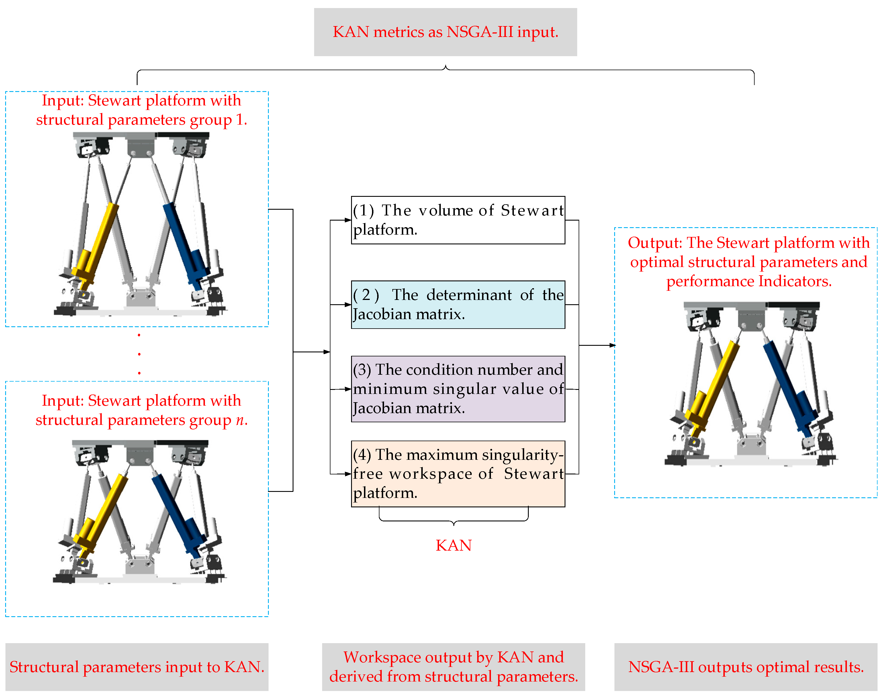
Figure 1. The overview of the proposed method.
Machines 13 00887 g001
Figure 2. The spatial position relationships of joint points in Stewart platform.
Machines 13 00887 g002
Figure 3. Geometric parameters of Stewart platform. (a) moving platform; (b) fixed platform.
Machines 13 00887 g003
Figure 4. The maximum and minimum lengths of driving rods are within stroke limit.
Machines 13 00887 g004
Figure 5. The minimum and maximum singular values in the Jacobian matrix.
Machines 13 00887 g005
Figure 6. Fifteen reference points on a normalized hyperplane for a three-objective problem (p = 4).
Machines 13 00887 g006
Figure 7. The schematic diagram of NSGA-III.
Machines 13 00887 g007
Figure 8. The flowchart of NSGA-III.
Machines 13 00887 g008
Figure 9. Schematic diagrams of MLP and KAN (a) MLP; (b) KAN.
Machines 13 00887 g009
Figure 10. The experimental Stewart platform YBT6-2000.
Machines 13 00887 g010
Figure 11. KAN vs. MLP Comparison Workflow [37].
Machines 13 00887 g011
Figure 12. Dynamic relationships and sensitivity trends of indicators F 1 F 6 with respect to design parameter R a .
Machines 13 00887 g012
Figure 13. Dynamic relationships and sensitivity trends of indicators F 1 F 6 with respect to design parameter R b .
Machines 13 00887 g013
Figure 14. Dynamic relationships and sensitivity trends of indicators F 1 F 6 with respect to design parameter θ a .
Machines 13 00887 g014
Figure 15. Dynamic relationships and sensitivity trends of indicators F 1 F 6 with respect to design parameter θ b .
Machines 13 00887 g015
Figure 16. Dynamic relationships and sensitivity trends of indicators F 1 F 6 with respect to design parameter d .
Machines 13 00887 g016
Figure 17. Comparison of calculation efficiency between KAN and the mathematical method.
Machines 13 00887 g017
Table 1. Joint point coordinates of moving and fixed platforms in YBT6-2000 (units: mm).
Chain 1Chain 2Chain 3Chain 4Chain 5Chain 6
X a −850.585850.585950.725100.139−100.139−950.725
Y a 606.717606.717433.270−1039.987−1039.987433.270
Z a 000000
X b −174.829174.8291416.2951241.465−1241.465−1416.295
Y b 1534.4581534.458−615.822−918.636−918.636−615.822
Z b −1399.760−1399.760−1399.760−1399.760−1399.760−1399.760
Table 2. Comparison of five metrics regarding accuracy for the train set.
KANMLP
R 2 MAEMAPEMSERMSE R 2 MAEMAPEMSERMSE
α 0.99650.01310.65800.00040.01920.85540.09235.21340.01540.1241
β 0.99570.01480.25430.00050.02280.76810.12982.28480.02830.1683
γ 0.99930.00970.06620.00030.01590.93110.09991.11110.02570.1603
x /mm0.99960.00720.07040.00010.00940.96880.06640.73220.00690.0830
y /mm0.99930.00810.06820.00010.01150.96340.06650.57700.00720.0851
z /mm0.99910.00870.13610.00010.01140.90350.09061.26650.01370.1169
Table 3. Comparison of five metrics regarding accuracy for the test set.
KANMLP
R 2 MAEMAPEMSERMSE R 2 MAEMAPEMSERMSE
α 0.99610.01330.56860.00040.01970.85510.08923.06750.01430.1197
β 0.99520.01561.18730.00060.02370.75430.130731.41810.02890.1699
γ 0.99930.00970.14170.00020.01560.93390.09501.57080.02350.1533
x /mm0.99950.00740.09160.00010.00980.96850.06440.51640.00640.0802
y /mm0.99930.00810.08000.00010.01140.96200.06530.62130.00690.0829
z /mm0.99900.00870.12270.00010.01150.89860.09151.18240.01360.1168
Table 4. Different structural parameters for the default parameters, NSGA-II and NSGA-III.
Default ParametersNSGA-IINSGA-III
R a (mm)1044.7971195.286966.856
R b (mm)1544.3861325.850956.069
θ a (°)117.3486.926
θ b (°)137.16810.088
d (mm)1399.7601724.2181160.285
Table 5. Comparison of six optimization indicators for default parameters, NSGA-II and NSGA-III.
Default ParametersNSGA-IINSGA-III
F 1 ( m m 3 )3.182 × 1093.582 × 1091.400 × 109
F 2 1.121 × 10462.439 × 10461.402 × 1045
F 3 1.432 × 10141.631 × 10146.990 × 1013
F 4 2.9313.4073.482
F 5 (°)32.55744.75647.537
F 6 ( m m ) 437.901650.974501.412
Table 6. The value of SP in NSGA-II and NSGA-III.
NSGA-IINSGA-III
SP0.0400.018
Disclaimer/Publisher’s Note: The statements, opinions and data contained in all publications are solely those of the individual author(s) and contributor(s) and not of MDPI and/or the editor(s). MDPI and/or the editor(s) disclaim responsibility for any injury to people or property resulting from any ideas, methods, instructions or products referred to in the content.