Finite Element Research of Cup Wheel Grinding Heat Based on Trochoid Scratch Model

Abstract

Grinding is a highly precise machining process. However, excessive temperatures during grinding can result in adverse thermal effects on the machined material. In this study, cup wheel grinding was analyzed using a model that represents heat generation as a trochoid discrete heat source formed by the interactions between abrasive particles and the workpiece surface. With this approach, certain assumptions were made to facilitate analysis, including the modeling of abrasive grains as rigid point heat sources. Finite element simulations and experimental validations based on the trochoid model were conducted using COMSOL 6.2 software. These analyses evaluated the thermal behavior of cup wheel grinding under varying wheel speeds and feed rate ratios. The results revealed an asymmetrical distribution of the temperature field in cup wheel grinding. By examining both surface and subsurface temperature fields, this study provided a more comprehensive understanding of grinding heat. Furthermore, this investigation explored the influence of trochoid trajectories and process parameters on the temperature field, highlighting intersection and curvature thermal effects. These findings contribute valuable analytical methods and theoretical insights for controlling grinding heat in precision machining processes.

1. Introduction

Grinding is a highly precise machining technique widely employed in advanced manufacturing sectors, including semiconductor wafer production and aerospace component fabrication [1]. However, the grinding process generates significant heat [2], which can lead to local temperature accumulation exceeding 1000 °C during single-crystal silicon surface grinding, making cooling challenging. The heat generated during grinding significantly impacts the mechanical properties of the workpiece [3,4]. When grinding temperatures surpass a critical threshold, thermal damage may occur on the workpiece surface [5], manifesting as surface burns [6], oxidation [7], residual stress development, and crack formation [8,9]. These defects degrade wear resistance, shorten component service life, and reduce fatigue strength. To mitigate the risks of thermal damage from excessive grinding temperatures and achieve high-precision, high-quality surface finishes, extensive global research has focused on thermal modeling in the grinding process.

Jaeger [10] established a theoretical framework to calculate temperature variations caused by a moving heat source in surface grinding. Outwater et al. [11] refined this model by incorporating energy partition coefficients in their analysis of the grinding temperature field. Bei [12] shifted the focus to a triangular heat source, offering deeper insights into the thermal field during grinding. Des Ruisseaux [13] extended this work by modeling the effects of convective heat transfer and surface cooling in the presence of a moving heat source. Malkin and colleagues [14,15] investigated the mechanisms of temperature rise and workpiece burns, focusing on the distribution of total energy among chip formation, plowing, and sliding processes. Rowe [16] proposed a thermal damage prediction model, introducing energy distribution coefficients of grinding. Jin [17] developed a grinding heat distribution model for inclined shapes to provide better insights into grinding temperature phenomena. Lin et al. [18] introduced the dynamic arc heat source model for cup wheel face grinding, analyzing the three-dimensional temperature field of the workpiece under dry conditions using heat conduction theory. Their theory was validated through numerical methods and experiments. Recently, Gao et al. [19] considered the cup wheel as a circular arc zone involved in grinding, and considered the variation in the cup wheel contact geometry on the temperature to complete the thermal modeling of cup wheel grinding. Many assumptions were made during the development of these models to simplify them, but they are still used to analyze the grinding heat problem, such as rail grinding [20,21].

Various approaches have been extensively employed to analyze grinding temperature fields. Finite element simulation, a widely used numerical method, has frequently been applied to study grinding heat. Zhang et al. [22] developed a numerical model using ANSYS 14.0 finite element software to address the challenges posed by an arc-shaped moving heat source in cup wheel grinding. Similarly, Dai et al. [23,24] constructed a grinding temperature field based on an annular, non-uniform heat source using finite element simulations. Mao et al. [25] compared the temperature fields of wet grinding surfaces using parabolic and triangular heat source models through the finite element method. However, these studies primarily relied on finite element simulations with different heat source geometries, which may not fully account for the abrasive heat source’s influence on the surface temperature field during grinding. For brittle materials, the finite element modeling of grinding heat primarily focuses on their unique thermal properties [26]. Due to their low thermal conductivity, heat accumulation is localized near the grinding zone, requiring precise consideration of heat transfer and thermal boundary conditions.

Grinding heat is generated at the macroscopic scale, resulting from material removal by abrasive particles [27,28]. Abrasive grain scratching experiments have become a key method for investigating material processing mechanisms [29]. The modeling of the actual trajectory of the abrasive grains by discrete abrasive grains helps in the study of grinding heat. Zhao et al. [30] proposed that the trajectory of the abrasive grains following the movement of the cup wheel on the surface of the workpiece is a trochoid. The trochoid model not only realizes the formation of high-speed cross scratches in continuous long scratches, but also reproduces the real working conditions of the interaction between the abrasive grains on the end face of the cup wheel and the workpiece. Again, this model can be well applied in the thermal study of discrete grit grinding of cup wheels. In a previous study, we established and validated an analytical model of the heat source at the intersection of trochoidal lines based on the theory of moving heat sources. However, the application of the trochoid model to analyze the numerical simulation of grinding heat of cup wheels still needs to be investigated. In this study, we aim to further investigate the thermal effects of cup wheel grinding using the trochoidal scratch model through finite element analysis. The numerical solutions from finite element simulations will provide deeper insights into the trochoidal effect, establishing a more reliable reference for grinding research and industrial applications.

2. The Establishment of Numerical Simulation Model

2.1. The Establishment of Trochoidal Scratch Model

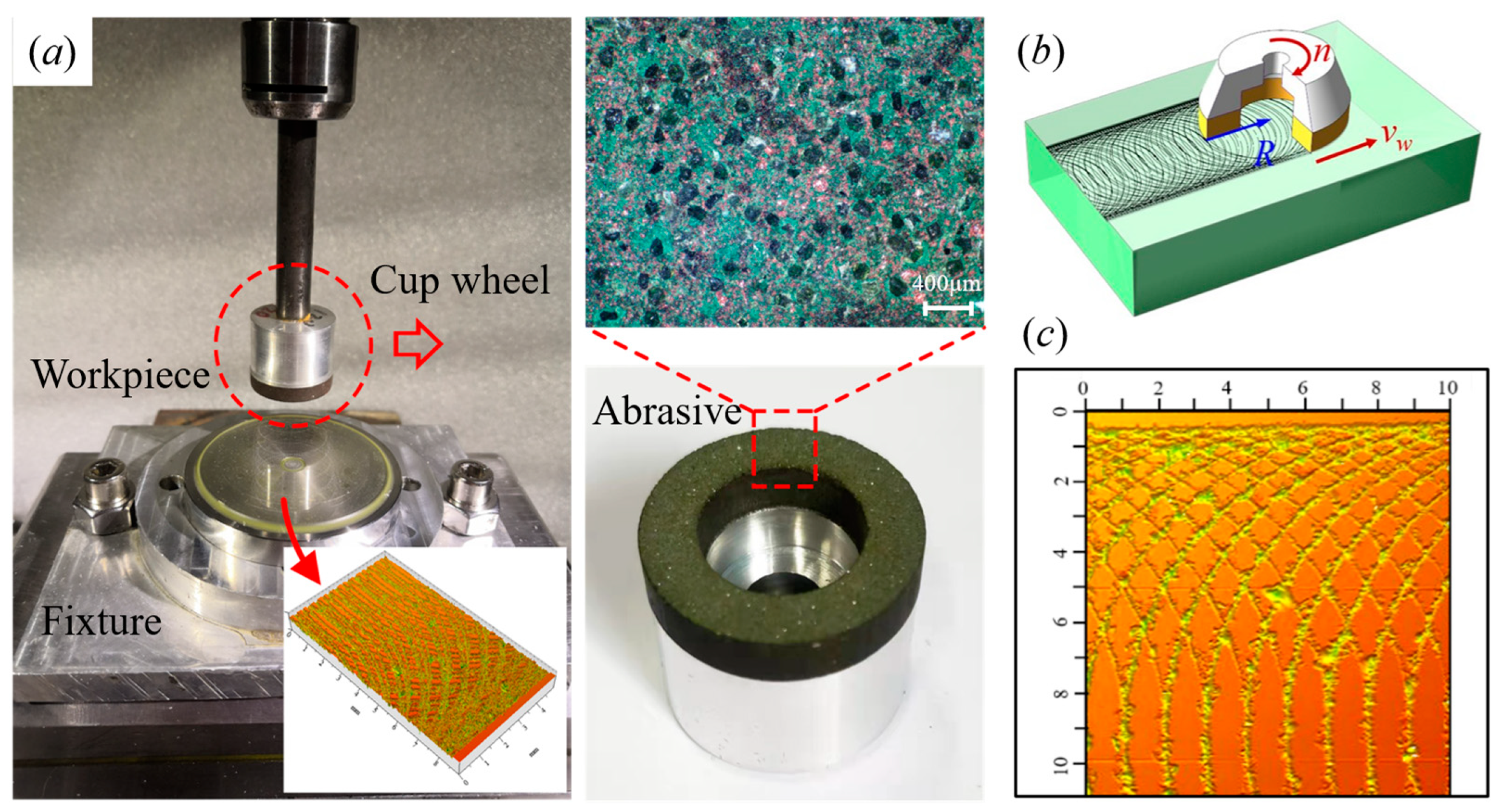
The cup grinding wheel is widely used for endface grinding of hard and brittle materials such as glass and ceramics due to its larger contact area, which enhances both precision and efficiency. As shown in Figure 1a, the cup wheel is mounted on a precision machining tool to grind the surface of quartz glass. The abrasive grains on the wheel’s end face vary in shape, height, and distribution, yet the spatial arrangement remains relatively stable due to the overall structure of the wheel. As illustrated in Figure 1b, when rotational speed and feed rate are kept constant, the surface texture produced by grinding is closely linked to the sequence in which the workpiece contacts the abrasive grains. The scratch patterns from different grains are consistent in form. Figure 1c shows the trajectory of the workpiece surface after grinding, measured using a three-dimensional surface topography tool. It reveals that while different abrasive particles leave marks in various locations on the workpiece, the overall trajectories exhibit uniformity across these positions.

End surface grinding with a cup wheel is characterized by the movement of multiple abrasive particles, each operating with a unique dynamic radius and advancement speed. This motion creates trochoidal patterns that result from the material processing. As shown in Figure 2a, the motion of individual particles on the cup wheel’s end face can be analyzed by breaking down their trajectories. Variations in curvature within a single grain’s path produce different trajectory patterns, corresponding to different radii, such as R₁ and R₂.

End surface grinding with a cup wheel requires a combination of rotational and linear movements of both the workpiece and the wheel. This interaction can be modeled as circular motion, where the wheel rotates with a base radius r, as shown in Figure 2b. The base radius r is defined as follows:

$$r={\displaystyle \frac{v_w}{\omega }}={\displaystyle \frac{v_w}{2\pi n}}$$

(1)

where v_w represents the linear feed rate of the workpiece, ω refers to the angular velocity of the grinding wheel as it rotates around the spindle, and n denotes the rotational speed of the grinding wheel. The complex motion of an individual abrasive grain due to the wheel’s rotation results in a motion equation describing its trajectory on the workpiece surface:

$$\left\{\begin{array}{l}x=\pm r\theta +R\sin \theta \\ y=R(1-\cos \theta )\end{array}\right.$$

(2)

where r represents the radius of the base circle, while R denotes the radius of the moving circle, which corresponds to the distance between the abrasive grain and the tool’s center. θ signifies the angle of rotation of the base circle, where “+” indicates a counterclockwise direction, and “−” signifies clockwise rotation.

As shown in Figure 2c, the surface grinding process using a cup wheel generates various trochoidal paths based on specific parameters, with the primary influences being the rotational velocity of the grinding wheel and the feed rate. The advantages of using a trochoidal scribe model for developing thermal theories in surface grinding are threefold. First, the trochoidal path represents the actual trajectory resulting from the grinding wheel’s relative motion against the workpiece, accurately reflecting real interaction conditions. Second, the adjustable scratch speed of the trochoidal scribe accommodates a range of grinding speeds, effectively minimizing damage from short duration impacts common in traditional high-speed grinding. Finally, the continuous crossing nature of trochoidal trajectories simplifies the formation of micro-surface cross scratches, offering an improvement over a conventional scratch pattern.

Figure 2d illustrates how a single abrasive grain generates intersections by following the cross-path of trochoidal scratches. The diamond grains rotate at a constant speed (n/rpm) in synchronization with the scratching tool, while the workpiece moves linearly at a velocity v_w, creating sub-trochoidal motion patterns on its surface in a clockwise sequence. Starting at point A, the trajectory follows ABCD clockwise while simultaneously advancing along BD. In the second to fifth cycles, (T = 2, 3, 4, 5). By analyzing these sequential paths, we then find some cycles showing cyclic changes. The results indicate that the trochoidal patterns feature multiple cross scratches, with intersections primarily concentrated in two regions (N-side and S-side). These paths exhibit cyclic properties, and the total number of intersections is closely related to the speed of the grinding wheel and the workpiece feed rate. As these parameters change, the positions and angles of the scratch intersections shift significantly. A higher ratio of wheel speed to feed rate leads to an increase in the number of cross scratches, which can be controlled by adjusting the process settings.

2.2. Finite Element Model Setup and Discretization

In the finite element model developed for this study, the grinding wheel and the workpiece interaction is comprehensively represented by modeling the grinding wheel as a collection of discrete abrasive grains. Each abrasive grain acts as an independent point heat source, which contributes to the material removal and heat generation during the grinding process. The point heat sources are distributed across the grinding wheel’s surface, accurately reflecting the random distribution of abrasive grains. To simulate the thermal effects, each point heat source is defined by its localized heat flux, which depends on the grinding parameters, including tangential grinding force and wheel speed. These heat fluxes are then applied incrementally to the workpiece surface following the trochoidal trajectories of the abrasive grains. This approach ensures that the grinding process’s thermal characteristics are captured accurately without oversimplifying the tool–workpiece interaction.

The model accounts for the cumulative thermal effects of all abrasive grains in contact with the workpiece. The distribution of these point heat sources effectively represents the grinding wheel’s active surface, thereby creating a complete numerical representation of the tool–workpiece system. The thermal boundary conditions, including the heat transfer coefficients and the convective environment, are also incorporated to simulate the heat flow at the interface accurately. It focuses on the thermal phenomena in cup wheel grinding, simplifying the mechanical–thermal coupling to isolate and analyze the heat generation and distribution caused by abrasive interactions. While the mechanical effects, such as deformation, strain rates, and their influence on heat conduction, are critical in practical grinding processes, the decoupling approach adopted here enables a more focused investigation of thermal behaviors under varying grinding parameters. Such simplifications are commonly employed as a foundational step in grinding heat analysis, providing insights that can later be integrated into coupled mechanical–thermal models.

Grinding involves a large number of abrasive particles. This interaction initiates several heat transfer processes within the material, which are critical in determining the final properties of the workpiece. The temperature distribution over space and time is typically modeled using a heat transfer equation, expressed by the following formula:

$$\rho C_P{\displaystyle \frac{\mathsf{\partial }T}{\mathsf{\partial }t}}={\displaystyle \frac{\mathsf{\partial }}{\mathsf{\partial }x}}\left(k{\displaystyle \frac{\mathsf{\partial }T}{\mathsf{\partial }x}}\right)+{\displaystyle \frac{\mathsf{\partial }}{\mathsf{\partial }y}}\left(k{\displaystyle \frac{\mathsf{\partial }T}{\mathsf{\partial }y}}\right)+{\displaystyle \frac{\mathsf{\partial }}{\mathsf{\partial }z}}\left(k{\displaystyle \frac{\mathsf{\partial }T}{\mathsf{\partial }z}}\right)+Q_{in}(x,y,z)$$

(3)

where T is the temperature, t is the time, x, y, z are the spatial coordinates, k is the import coefficient, C_p is the constant pressure thermal fusion, ρ is the density; discretize its time direction as follows:

$${\displaystyle \frac{\mathsf{\partial }T}{\mathsf{\partial }t}}\approx {\displaystyle \frac{T_{i,j,k}^{n+1}-T_{i,j,k}^n}{\mathrm{\Delta }t}}$$

(4)

The discretization of its x, y, z three-dimensional spatial directions can be obtained, respectively:

$$\begin{array}{l}{\displaystyle \frac{{\mathsf{\partial }}^{2}T}{\mathsf{\partial }{x}^2}}\approx {\displaystyle \frac{T_{i+1,j,k}^n-2T_{i,j,k}^n+T_{i-1,j,k}^n}{\mathrm{\Delta }{x}^2}}\\ {\displaystyle \frac{{\mathsf{\partial }}^{2}T}{\mathsf{\partial }{y}^2}}\approx {\displaystyle \frac{T_{i,j+1,k}^n-2T_{i,j,k}^n+T_{i,j-1,k}^n}{\mathrm{\Delta }{y}^2}}\\ {\displaystyle \frac{{\mathsf{\partial }}^{2}T}{\mathsf{\partial }{y}^2}}\approx {\displaystyle \frac{T_{i,j+1,k}^n-2T_{i,j,k}^n+T_{i,j-1,k}^n}{\mathrm{\Delta }{y}^2}}\end{array}$$

(5)

The results of the temporal and spatial direction discretization are substituted into the original equations, which are displayed in the following format:

$$T_{i,j,k}^{n+1}=T_{i,j,k}^n+{\displaystyle \frac{\mathrm{\Delta }t}{\rho C_p}}\left[k\left({\displaystyle \frac{T_{i+1,j,k}^n-2T_{i,j,k}^n+T_{i-1,j,k}^n}{\mathrm{\Delta }{x}^2}}+{\displaystyle \frac{T_{i,j+1,k}^n-2T_{i,j,k}^n+T_{i,j-1,k}^n}{\mathrm{\Delta }{y}^2}}+{\displaystyle \frac{T_{i,j,k+1}^n-2T_{i,j,k}^n+T_{i,j,k-1}^n}{\mathrm{\Delta }{z}^2}}\right)+Q_{in}\right]$$

(6)

Q_in is the abrasive grains transfer to the workpiece substrate.

$$Q_{in}=R_w{Q}_{AVG}t$$

(7)

where Q_AVG represents the average power of the heat source from the abrasive grain, while t refers to the grinding duration of the abrasive grain in seconds. During wheel grinding, not all the generated heat is transferred to the material due to losses from convection and conduction. Therefore, a coupling efficiency R_w is introduced to account for this. Under dry grinding conditions, heat transfer primarily occurs between the tool and the material. The heat transfer efficiency can be computed using the Hahn model [31] through the following equation:

$$R_w={\displaystyle \frac{k_1}{k_1+k_2}}$$

(8)

where k₁ represents the thermal conductivity of the workpiece, while k₂ corresponds to the thermal conductivity of the grinding wheel. The heat flux generated by the grinding wheel is modeled as the cumulative effect of individual abrasive grains, each represented by a Gaussian heat source. This approach reflects the statistical distribution of grain dimensions, as the height and diameter of grains within a specified grit size are known to follow a normal distribution. By modeling each grain as a Gaussian heat source, we effectively capture the localized thermal intensity variations due to individual grain interactions with the workpiece. The average intensity of the heat source for each abrasive grain is as follows:

$$Q_{AVG}(x,y,z,t)={\displaystyle \frac{2P}{\pi r^2}}\exp \left(-{\displaystyle \frac{2({(x-x_0)}^2+{(y-y_0)}^2)}{r^2}}\right)\delta (z-z_0)$$

(9)

where P is the energy power of the abrasive grain heat source on the surface of the workpiece, r is the radius of the abrasive grain heat source, (x₀, y₀, z₀) is the position where the abrasive grain heat source is located, and the Dirac function δ ensures that the abrasive grain heat source has the desirable localization properties in the vertical direction, which is extremely important for simulating the thermal effect of abrasive grains, and for depth control, it is extremely important. The input energy P of the abrasive heat source is related to the grinding force, which is related to the process parameters as follows:

$$P=F_t\cdot v_s$$

(10)

where F_t is the tangential force of grinding and v_s is the linear speed of the grinding wheel speed. The grinding force is related to the parameters of the grinding process; for cup wheel grinding, the grinding force can be expressed as follows:

$$F_n=K{C}^r{\left(v_w/v_s\right)}^{2\epsilon -1}{a_p}^{\epsilon }{D}^{1-\epsilon }$$

(11)

$$F_t=\mu \cdot F_n$$

(12)

The grinding wheel plays a crucial role in determining the distribution and intensity of the heat generated during the grinding process. The active surface of the grinding wheel, which consists of numerous abrasive grains, significantly influences the heat source intensity and the subsequent temperature distribution in the workpiece. The abrasive grains on the grinding wheel surface are typically irregularly distributed, with a range of grain sizes and densities. The size of the grains directly influences the contact area with the workpiece and, consequently, the intensity of the heat generated. Larger grains typically result in a more concentrated heat source, while smaller grains contribute to a more diffuse heat distribution. The protrusion height of the abrasive grains determines the actual contact area between the grinding wheel and the workpiece. Grains with higher protrusion contribute more significantly to the heat flux, while those with lower protrusion have a reduced effect on the local heat generation. The variation in grain protrusion introduces additional variability in the heat source intensity across the grinding wheel’s active surface. During the grinding process, the abrasive grains undergo wear and fracture, leading to changes in the grinding wheel’s active surface over time. These changes affect both the grain size and the distribution, as well as the protrusion height of the grains.

The grinding wheel used in this study is a resin-bonded diamond cup wheel with abrasive grain sizes ranging from 100 to 200 μm. Diamond is selected as the abrasive material for its exceptional hardness, thermal conductivity, and wear resistance, making it well suited for precision grinding. The resin binder ensures that the grains are securely held while providing a compliant structure that can withstand grinding forces. For modeling purposes, the grains are assumed to be uniformly distributed across the active surface of the grinding wheel. Each grain is approximated as a spherical particle with sharp edges to simulate its cutting action and heat generation during grinding. The estimated grain density is 25 grains per mm², calculated based on the wheel’s active surface area and average grain size. In the numerical model, the grinding wheel is treated as a rigid body due to its high stiffness and negligible deformation under normal grinding conditions. This assumption simplifies the computation while retaining the model’s validity for simulating heat generation and distribution.

For different grinding process parameters, the grinding force can be determined by the above equation which in turn determines the grinding input power and the intensity of the input heat source. For the analysis of transient heat transfer during the grinding process, the following initial conditions must be set:

$$T{(x,y,z)}_{t=0}=T_0$$

(13)

where T₀ refers to the initial or ambient temperature. The boundary conditions at the free surface can be defined as follows:

$$k_n{\displaystyle \frac{\mathsf{\partial }T}{\mathsf{\partial }N}}=q(x,y,z,t)+h_c(T-T_0)$$

(14)

where N represents the normal vector applied to the heat flow surface, influenced by the external heat source and the convective environment. k_n is the thermal conductivity in the direction perpendicular to the surface. q indicates the localized heat flow from the higher temperature region to the lower temperature region of the workpiece. h_c refers to the convective heat transfer coefficient.

To validate the model, this study focuses on quartz glass, a representative hard and brittle material commonly used in precision manufacturing. Quartz glass is selected due to its unique grinding mechanisms, which involve micro-deformation, micro-cracking, and micro-chip formation, making it an ideal case for demonstrating the model’s capability. By incorporating the thermal properties of quartz glass into the simulations, we demonstrate the model’s effectiveness in predicting temperature distributions during grinding. The workpiece is made of quartz glass, with dimensions of 100 mm × 100 mm × 10 mm.

Table 1. Basic physical parameters of workpiece and grinding wheel.

Basic Physical Parameters	Value
Density of workpiece ρ(T) [kg/m3]	2200 × (1 − 5.5 × 10−7 × (T − 300))
Thermal conductivity of workpiece k1(T) [W/(m·K)]	1.4 − 2.5 × 10−4 × T
Thermal conductivity of wheel k2(T) [W/(m·K)]	8.4 − 6.3 × 10−4 × T
Thermal diffusivity of workpiece a(T) [m2/s]	0.55 × 10−6 + 1.2 × 10−9 × T
Heat capacity of workpiece Cp(T) [J/(kg·K)]	740 + 0.1 × T
Young’s modulus of workpiece E(T) [GPa]	72 − 0.017 × T
Yield strength of workpiece σY(T) [GPa]	1.1 × exp(−0.0015⋅T)
Compliance coefficients of workpiece [Pa−1]	S11(T) = 1/(72 − 0.017⋅T) S12(T) ≈ −0.17/(72 − 0.017⋅T) S44 ≈ (1 + 0.17)/(2⋅(72 − 0.017⋅T))

provides the thermal and physical properties of quartz glass at room temperature. A resin-bonded diamond cup wheel, with an outer diameter of 50 mm, is used for grinding. The grinding process is conducted under dry conditions. Material properties depend on temperature. Key parameters, including thermal conductivity, heat capacity, thermal diffusivity, and density are represented as functions of temperature (T). These dependencies account for the significant changes in material behavior under varying thermal conditions, particularly in high-temperature regions.

The thermal behavior during grinding is highly complex, necessitating several assumptions to simplify the numerical calculations for estimating temperature distribution in the workpiece. These assumptions include uniform and constant heat generation within the contact zone between the grinding wheel and the workpiece, with heat conduction being the sole mode of heat transfer in this region. Air convection is neglected in the contact zone but accounted for in other areas of the workpiece. The finite element model operates within a three-dimensional framework, directly simulating the heat transfer from the abrasive grains to the workpiece surface. No spatial state reduction was performed; instead, the heat flux generated by the grains follows the trochoidal trajectory directly on the three-dimensional workpiece surface. This approach assumes negligible vertical displacement of the grinding wheel relative to the workpiece, a hypothesis supported by the dominant thermal effects observed in the grinding zone. The abrasive grains are treated as rigid bodies in the simulation, reflecting their high stiffness and hardness compared to the workpiece material. The grain distribution and size remain constant throughout the simulation, as grain breakage was not included in this study.

Using the defined parameters and assumptions for the temperature field model, the numerical simulations were conducted in COMSOL Multiphysics (Version 6.2) using the Heat Transfer in Solids module. Given the complexity of the grinding process and the continuous nature of the model, an analytical solution was infeasible. Therefore, a numerical approach was employed. Temperature boundary conditions were applied to simulate heat partitioning between the grinding wheel and the workpiece. While thermal contact resistance was not explicitly modeled in this study, predefined heat partition coefficients based on empirical data were used to approximate heat flow at the interface. Heat flux boundary conditions were defined as Gaussian distributions corresponding to the localized heat input from the abrasive grains. These heat sources followed trochoidal trajectories determined by the grinding parameters. Figure 3a shows the model of the trochoidal heat source applied to the workpiece surface. The heat flux is incrementally applied over continuous time, allowing the abrasive heat source to move across the surface following the predefined path. The governing transient heat transfer equation was solved iteratively, accounting for time-dependent heat input from the grinding process.

The mesh density is set to be highest on the grinding surface and gradually decreases as the distance from the surface increases, depending on the grinding conditions. This meshing strategy ensures both accuracy and reduced computation time. The exaggerated grid structure is shown in Figure 3b. The cell size was determined based on a convergence study and the feasibility of the computational method. Figure 4 illustrates the computational process for the trochoidal moving heat source. The simulations employed a direct solver with adaptive time-stepping to ensure numerical stability. Convergence criteria were set for both temperature field and heat flux, with a relative tolerance of 10⁻⁶ to guarantee accurate results.

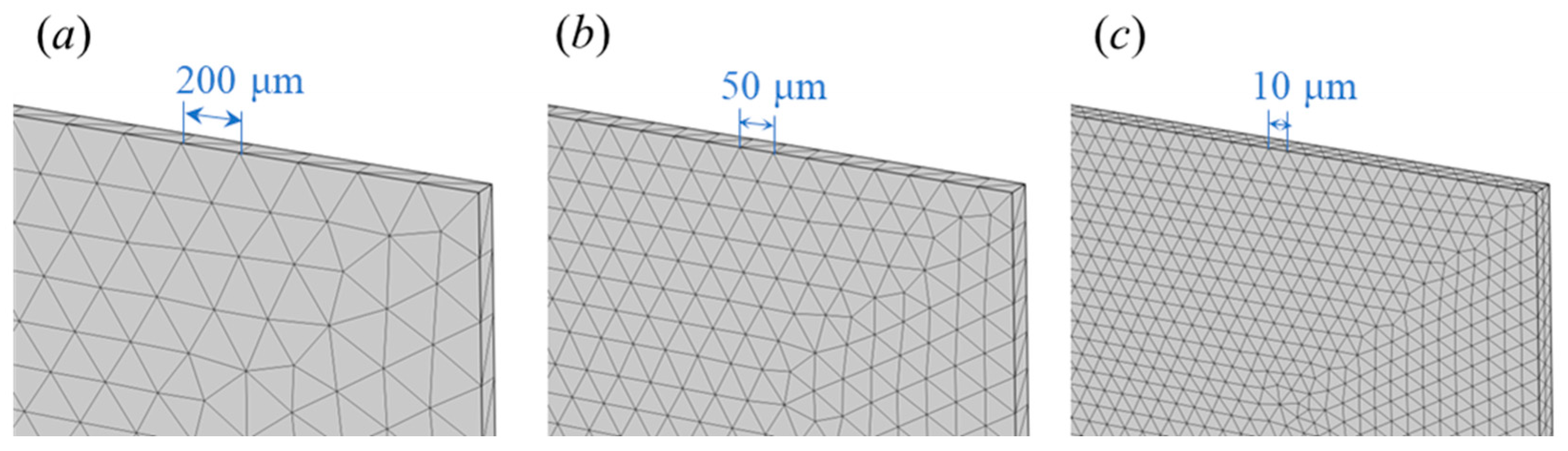
The accuracy of the model is significantly influenced by factors such as finite element software settings, grinding parameters, and heat source intensity. This study examines how these parameter settings affect both analytical and numerical models, following a similar approach to that found in the literature [22]. The element size on the top surface of the workpiece directly impacts the smoothness of the temperature gradient and the element’s heat capacity. Figure 5 shows the variations in temperature distribution resulting from different element size configurations. Larger element sizes introduce errors in the thermal dynamic response, while smaller sizes rapidly increase mesh partitioning, leading to a substantial file size. In this study, an element size of 10 μm is considered sufficient. The finite element model discretizes the workpiece using a structured mesh, with approximately 100,000 finite elements and 300,000 degrees of freedom. The simulations employed a time-dependent direct solver with adaptive time-stepping. The initial time step was set to 0.01 s, with a relative tolerance of 1 × 10⁻⁶, ensuring both stability and precision. The mesh density is highest in the grinding zone to capture the localized thermal effects of the abrasive grains. Adaptive meshing techniques were used to ensure computational efficiency while maintaining accuracy in regions of steep thermal gradients. The grinding wheel is represented implicitly as a series of point heat sources that move along predefined trochoidal paths. This approach captures the thermal interactions between the tool and the workpiece without the need for explicit meshing of the wheel. Each heat source is oriented normal to the workpiece surface, simulating the dominant interaction geometry of the abrasive grains during grinding. To ensure coherence in the thermal simulation, the heat flux continuity across adjacent regions was carefully calibrated. This ensures accurate modeling of transient heat transfer from the moving heat sources to the workpiece surface.

The proposed finite element model for grinding heat analysis is designed with a general methodology that can be applied to various material types, including brittle and ductile materials. The model focuses on the heat generation and distribution induced by the abrasive heat source, without explicitly considering material-dependent mechanical properties, such as plastic deformation or fracture toughness. Instead, it centers on the thermal interactions at the grinding surface, driven by process parameters such as feed rate and spindle speed. This general approach allows for broad applicability, provided the relevant thermal and physical properties of the material are input into the simulation.

3. Experimental Design and Verification

To validate the grinding thermal model based on trochoidal scratch theory, an experimental verification of the grinding heat generated by the cup wheel was conducted. As shown in Figure 6, the experiment utilized the spindle of an optical curve grinder to mount the cup wheel, with a machine-specific fixture designed to secure the workpiece. The cup wheel used was a resin-bonded diamond grinding wheel with a diameter of 50 mm. The grinding wheel used in this study is a resin-bonded diamond cup wheel with abrasive grain sizes ranging from 100 to 200 μm, as measured through microscopic imaging. The average protrusion height of the grains was determined to be approximately 30 μm using a surface profilometer, and the grain density was estimated to be 25 grains per mm² based on the wheel’s active surface area and grain size. The active surface of the grinding wheel, the outer diameter of the grinding wheel, is 50 mm, the inner diameter of the grinding wheel is 45 mm, the grinding wheel area is 372.875 mm² and was estimated to contain approximately 9322 grains, calculated based on its surface area and grain density. The grinding wheel’s binder material is resin, which provides a compliant yet robust matrix for securing the grains and contributes to the thermal dissipation characteristics of the wheel. The grain distribution on the grinding wheel’s surface was inherently random, as is typical in industrial applications, and the resin binder ensured strong adherence of the grains while allowing for slight variability in grain orientation. The spatial arrangement and random distribution of the abrasive grains were analyzed using profilometry to inform the heat source modeling. These factors, including grain size, density, and protrusion height, were incorporated into the finite element model by calibrating Gaussian heat flux distributions for each abrasive grain to accurately represent the thermal interactions during grinding.

The workpiece, made of quartz glass, measured 100 mm × 100 mm × 10 mm. This size was chosen to validate the finite element model by providing a controlled experimental setup for measuring temperature distributions during grinding. The thickness of 10 mm ensures accurate representation of heat transfer dynamics within the workpiece while minimizing edge effects that could impact the results. Prior to the experiment, the workpiece was cut, and a thermocouple was embedded in the seam of the workpiece, which was then affixed using epoxy resin. The grinding temperature was measured using the thermocouple, which was connected to a data collector that transmitted the data to a computer.

This scratch trajectory is primarily influenced by the rotational velocity of the grinding wheel and the feed rate of the workpiece. As a result, the speed of the grinding wheel and the feed rate directly affect the temperature distribution within the grinding zone on the cup wheel’s surface. Equation (2) demonstrates that, when the radius of the moving circle R remains constant, the minimum morphological feature unit of the trochoid is identical, provided the ratio of the workpiece feed rate v_w to spindle speed n is the same, regardless of differing values of n and v_w. This means the geometries of the trochoidal trajectories are completely consistent. The difference lies in the change in curvature of the trochoidal trajectory, which is caused by variations in spindle speed and feed rate, and the change in cutting speed of the abrasive grains v_s in the trochoidal scratches. Therefore, the effect of the trochoidal trajectory on the grinding heat of the cup wheel can be studied by varying the workpiece feed rate v_w without altering the spindle speed n. As shown in Figure 7, by changing only the workpiece feed rate, while keeping the rotational speed of the grinding wheel constant, the sparsity of the abrasive grain heat source trajectory, the number of intersections, and the curvature change significantly.

At different grinding depths, the energy expended by the wheel grinding the material varies, leading to changes in the intensity of the heat source. As shown in

Table 2. Parameter setting of experiment and simulation.

No.	Grinding Depth (ap)	Spindle Speed (vs)	Feed Speed (vw)
1	15 μm	13.08 m/s	1 mm/s
2	15 μm	13.08 m/s	2.5 mm/s
3	15 μm	13.08 m/s	5 mm/s
4	15 μm	13.08 m/s	7.5 mm/s
5	15 μm	13.08 m/s	10 mm/s
6	5 μm	13.08 m/s	1 mm/s
7	10 μm	13.08 m/s	1 mm/s
8	20 μm	13.08 m/s	1 mm/s
9	30 μm	13.08 m/s	1 mm/s

, a one-factor method was employed to select parameter settings for studying the influence of process parameters on the workpiece surface grinding temperature. Typical feed rate parameters from groups 1 to 5 were used to examine the effect of the workpiece feed rate (v_w) on the grinding temperature. Additionally, process parameters from groups 6 to 9 were used to investigate the impact of grinding depth (a_p) on the workpiece surface temperature. A broad range of parameter settings, including both high and low speeds, as well as variations in grinding depth, were applied in this study to ensure generality of the findings.

4. Results and Discussion

4.1. Comparison of Numerical Modeling and Experimental Results

The random distribution of grains was accounted for by conducting multiple trials under identical conditions, allowing for average grinding temperature statistical validation of the results. This experimental design ensures the findings are robust and reflective of industrial grinding conditions. By comparing the experimental results with the finite element model, as shown in Figure 8a–c, the grinding temperature consistently increases as the grinding depth increases. Quantitatively, the simulation results closely match the experimental data, with an average error of approximately 5 °C and a maximum deviation of 10 °C. Notably, the discrepancies are more pronounced at greater grinding depths, which may be attributed to simplifications in the simulation model, such as material properties and idealized boundary conditions, which fail to account for localized thermal effects.

As illustrated in Figure 8d–f, the grinding temperature initially decreases and then increases with rising feed speeds. The maximum observed error between experimental and simulation data is 8 °C. The deviation is more significant at lower feed speeds, which may result from variations in heat dissipation and thermal gradients that are not fully captured by the simulation. Additionally, potential errors in temperature measurement, such as the response time and positioning of thermocouples, could further contribute to this discrepancy.

The proposed finite element model incorporates a detailed representation of the grinding wheel’s active surface through the distribution of discrete point heat sources. This modeling approach allows for an accurate simulation of the thermal interaction between the grinding wheel and the workpiece. The comparison of numerical and experimental results shows good agreement, validating the effectiveness of this model in capturing the grinding process’s thermal behavior. By treating the grinding wheel as a collection of point heat sources, the model captures the heat flux distribution and its impact on the workpiece’s temperature field. The experimental results corroborate the predicted temperature field, with an average error of approximately 5 °C. This level of accuracy demonstrates that the model successfully simulates the complex interactions between the grinding wheel and the workpiece. The discretization strategy employed in this study balances computational efficiency with accuracy. The fine mesh in the grinding zone captures the localized thermal effects of the abrasive grains, while the total degrees of freedom ensure a detailed simulation of transient heat transfer. The detailed numerical configuration in COMSOL Multiphysics provides a robust framework for simulating the thermal effects of the grinding process. Mesh refinement, adaptive time-stepping, and accurate boundary condition definitions ensure the reliability and reproducibility of the proposed model. The agreement between experimental and simulation results validates the accuracy of this computational approach.

Meanwhile, the numerical model in this study incorporates several simplifications to facilitate the analysis of thermal effects during grinding. While these assumptions enable computational efficiency and focus on dominant heat transfer mechanisms, they may introduce limitations. Representing abrasive grains as point heat sources simplifies the heat flux input but does not account for the actual geometry of the grains. This could lead to localized inaccuracies in predicting temperature gradients near the grain edges. However, the overall temperature distribution remains consistent with experimental results, suggesting that the simplification is valid for capturing macroscopic thermal effects. The assumption of rigid abrasive grains excludes deformation and elastic recovery effects, which can influence the contact area and, consequently, the heat flux distribution. In scenarios involving high contact pressure, this could lead to slight underestimation of the peak temperature values. Grain breakage and wear were not modeled, as this study focuses on static grain properties. While this omission limits the model’s applicability to long-term grinding processes, it does not significantly affect the short-term thermal phenomena analyzed in this work. Despite these simplifications, the agreement between experimental and numerical results demonstrates that the model accurately captures the dominant thermal behavior during grinding.

Overall, the trends in grinding temperature between the experimental and simulation results are consistent across all examined parameters. These findings confirm the validity of the finite element grinding thermal model based on trochoidal scratch theory in capturing the thermal characteristics and influencing factors of cup wheel grinding, providing a solid foundation for subsequent optimization studies. To further understand the grinding thermal characteristics of discrete grit cup wheels, we will simulate the surface temperature variation by single-grit finite element simulation and multi-grit finite element simulation. The influence of trochoid process parameters on the grinding heat distribution and the problems caused by the trochoid effect in grinding heat will be further analyzed.

4.2. Influence of Trochoid Trajectory Process Parameters on Grinding Heat

As shown in Figure 9, the workpiece feed rate (v_w) significantly affects the grinding temperature over time. Variations in feed rate alter the density of the heat source path generated by the abrasive grains, resulting in different temperature field distributions across the surface. At low feed rates, the temperature gradient on both sides of the workpiece remains relatively uniform. However, as the feed rate increases, the changes in the surface temperature gradient become more pronounced. At a certain feed rate, the temperature field distribution across the surface becomes uniform over time due to internal heat transfer and diffusion within the workpiece. Once thermal equilibrium is reached, the temperature distribution stabilizes. At higher feed rates, the heat source trajectory becomes sparser, preventing significant surface temperature accumulation, with the grinding heat concentrated around the abrasive grain path.

As the grinding depth varies, the intensity of the abrasive heat source becomes a key factor in influencing the distribution of the surface grinding temperature field. According to Figure 10, when comparing surface temperature distributions at a constant feed rate, the temperature on the workpiece surface increases significantly as the heat source intensity rises. The temperature distribution is primarily concentrated along the heat source’s path, with higher temperatures on both sides of the workpiece compared to the center. This uneven distribution aligns with the trochoidal trajectory of the abrasive grains. Furthermore, as the heat source intensity increases, heat transfer within the workpiece accelerates, leading to faster diffusion of heat across the surface. The greater heat source strength also amplifies the temperature difference between the source and the workpiece, raising the temperature gradient and further speeding up the heat transfer process.

When the transversal line is positioned in the center of the workpiece, the temperature along the line shows noticeable zigzag fluctuations over time, as shown in Figure 11. These fluctuations are primarily caused by the intersection of heat source tracks, which leads to localized temperature increases.

The subsurface grinding temperature field distribution allows for further investigation of the effects of grinding heat on the interior of the workpiece. As shown in Figure 12, the temperature distribution from the surface to the interior at different depths (d_p), under the same feed rate, clearly demonstrates the influence of surface temperature on subsurface temperature. At a feed rate of 1 mm/s, the slow feed rate causes the heat source trajectory of the abrasive particles to be relatively concentrated, resulting in higher temperatures inside the workpiece compared to the surface. Due to convection heat dissipation, the surface temperature dissipates quickly when exposed to air, while inside the workpiece, heat conduction leads to the accumulation of heat. As illustrated in Figure 12a–f, the surface temperature is the highest, and as the depth of the cut increases, the maximum temperature decreases from 470 K to 407 K, showing a consistent downward trend in the temperature field.

4.3. Analysis of Trochoidal Effect in Grinding Heat of Cup Wheel

At a workpiece feed rate of 1 mm/s, the heat source trajectory of the abrasive grains is relatively concentrated due to the slow feed rate. Figure 13a–d show that the temperature on the edge of the surface is higher than in the center. As grinding continues, heat accumulates, causing a steady increase in surface temperature. Figure 14 presents the temperature distribution along the horizontal and vertical transversals of the workpiece surface. In the horizontal direction (x-axis), the temperature is highest in the regions where the grinding wheel passes, with the grinding zone temperature exceeding that of the rest of the surface. In the vertical direction (y-axis), the temperature on both sides is higher than in the middle, and one side consistently shows a higher temperature than the other.

In actual grinding, the random distribution and variability of abrasive grains on the grinding wheel’s active surface can lead to non-uniform heat generation during the grinding process. Each individual grain acts as an independent heat source, and the total heat flux is determined by summing the contributions of all grains on the active surface. This random distribution results in significant variations in heat source intensity, leading to localized temperature gradients within the workpiece.

Larger and more protruding grains tend to generate higher localized heat fluxes, which can create hot spots on the workpiece surface. These hot spots are primarily located where clusters of high-protrusion grains contact the workpiece. The intensity of the heat generated by these grains can lead to localized temperature spikes, which affect the surface integrity of the workpiece.

In addition to localized hot spots, the grinding process itself introduces asymmetry in the temperature distribution. As the grinding wheel moves across the workpiece, the relative motion between the wheel and the workpiece results in an uneven distribution of heat flux in the plane parallel to the wheel’s motion. This motion-induced asymmetry is further amplified by the random distribution of grains, which leads to skewed heat generation in certain regions of the contact area.

As shown in Figure 15a–c, at a workpiece feed rate of 5 mm/s, the crossing points of the trochoid trajectory become more pronounced due to the increased ratio of workpiece feed rate to spindle speed. The occurrence of cross-trajectories from the abrasive heat source leads to significantly higher temperatures at the crossing points compared to other areas, a phenomenon referred to as the “cross-point thermal effect”. This effect arises from the superposition of heat sources on the workpiece surface, resulting in localized heat accumulation. At this feed rate, the number of intersection points formed by abrasive particles on both sides of the workpiece varies, and the crossing angles of the scratches are not uniform. More crossings occur on the upper side of the workpiece than on the lower side, making the cross-point thermal effect the primary cause of the asymmetric temperature distribution on both sides of the workpiece.

As shown in Figure 15d–f, the change in curvature of the trochoid trajectory becomes more pronounced at a workpiece feed rate of 10 mm/s. The faster movement of the abrasive grain heat source per unit time increases the generation of grinding heat due to the interaction between the abrasive grain and the workpiece. A greater curvature in the trajectory results in a shorter distance traveled by the abrasive grain heat source per unit time and a longer duration of heat source action, leading to higher surface grinding temperatures in areas with greater curvature.

We observed that the intersection point and trajectory curvature significantly influence the surface grinding temperature. Based on this, two sets of typical process parameters were selected and further analyzed using numerical methods. As shown in Figure 16, when the abrasive heat source tracks intersect, the grinding temperature at the intersection point is notably higher than at other locations. Additionally, when the trajectory curvature of the abrasive heat source is large, the temperature distribution along the trajectory initially increases and then decreases.

In grinding processing, the grinding wheel grits ratio of the velocity to feed speed is typically between 60 and 80. As a result, workpiece feed speed to the spindle speed is less than 1 during actual grinding, indicating that the trajectory of the diamond grits in the cup wheel in actual grinding is trochoid. The cross-point thermal effect and curvature thermal effect will be widespread in cup grinding wheel endface grinding, and these two effects play an important role in this study with grinding temperature.

Under varying ratios of workpiece feed rate to spindle speed, both the cross-point thermal effect and the curvature thermal effect can be observed. When the ratio is low, the cross-point thermal effect is more pronounced, while a higher ratio emphasizes the curvature thermal effect. Therefore, the thermal effects of the trochoid manifest as the dynamic evolution of these two effects, depending on the ratio of workpiece feed speed to spindle speed. By controlling the trochoidal trajectory and process parameters, the distribution of the surface grinding temperature field can be managed, offering a potential solution for studying and mitigating heat generation in cup grinding wheel operations.

5. Conclusions

In this paper, we establish a finite element model that comprehensively incorporates the interaction between the grinding wheel and the workpiece by representing the abrasive grains as a distribution of point heat sources. This modeling approach provides a complete numerical representation of the grinding process, capturing both the localized and cumulative thermal effects of the abrasive grains. The numerical solution is obtained through finite element simulation using COMSOL 6.2 software. The simulation analyzes the temperature field distributions on the workpiece’s grinding surface and subsurface under varying feed rate-to-spindle speed ratios and different heat source intensities. The analysis identifies three key thermal effects: intersection, curvature, and trochoidal effects, all of which are associated with the grinding heat. The following conclusions are drawn from this study:

(1) Experimental and numerical results reveal that the grinding temperature increases with greater grinding depth and decreases with higher feed rates. These findings confirm the significant influence of process parameters on heat generation and dissipation during grinding. The numerical model demonstrated strong agreement with experimental results, with an average temperature prediction error of 5 °C and max temperature prediction error within 10 °C. This validates the model’s accuracy in capturing the thermal behavior of cup wheel grinding under varying process conditions.

(2) The trochoidal motion of abrasive grains generates localized heat accumulation at trajectory intersections, leading to the “cross-point thermal effect”. This effect was observed to dominate at lower feed rates, where the density of heat source paths is higher. Conversely, at higher feed rates, the “curvature thermal effect” becomes more prominent, as increased trajectory curvature intensifies heat accumulation in specific regions.

(3) Cup wheel endface grinding exhibits a coupling effect involving the sparseness of the abrasive grain heat source trajectory, the number of intersections, intersection angles, and curvature variations. Due to the uneven distribution of intersection points and curvature, the temperature field on the grinding wheel’s surface shows higher temperatures on both sides compared to the middle. Additionally, one side of the wheel experiences higher temperatures than the other. The thermal effects of the trochoid model are decoupled through analytical modeling and experimental quantification.

(4) The findings provide actionable insights for optimizing grinding parameters to minimize thermal damage and improve surface quality. The proposed model is generalizable to other resin-bonded diamond grinding wheels with similar grain sizes and densities. Future work could extend the model to account for more complex wheel geometries and abrasive grain wear dynamics.