Topology-Aware Efficient Path Planning in Dynamic Environments

Abstract

This study presents a path-planning approach toward efficient obstacle avoidance in dynamic environments. The developed approach features the awareness of the topological structure of the dynamic environment at a planning instant. It is achieved by employing a homology class path planner to generate a set of non-homotopy global paths. The global paths are cast into tree structures separately and optimized by the developed sampling-based path-planning methods. This mechanism can adaptively adjust the optimizing step size according to the change in the dynamic environment, and the sampling module uses the Gaussian Mixture Model (GMM) Optimizer to control the sampling space. The approach seeks the globally optimal path as it maintains and optimizes homology classes of admissible candidate paths of distinctive topologies in parallel. We conduct various experiments in dynamic environments to verify the developed method’s effectiveness and efficiency. It is demonstrated that the developed method can perform better than the state of the art.

1. Introduction

In recent decades, robot path planning in dynamic environments has become an essential issue in robotics research [1]. In the human–robot coexisting environment, it is necessary to ensure that the robot can successfully navigate in some complex environments [2,3]. The path planner deals with non-static scenarios, where crowds of pedestrians and dynamic obstacles regularly invalidate paths generated by using standard approaches. Once a path is invalidated in a dynamic environment, a new path has to be re-generated. Having a set of precomputed distinct paths is a more reasonable topological structure approach than replanning the path for each environment’s change. A homology class is defined by a set of paths with the same start and goal points which can be continuously deformed into one another without intersecting obstacles. The cross-entropy (CE) method is integrated with modern optimal motion planning techniques, such as the Rapidly Exploring Random Tree (RRT), to address complex environments.

Almost all path-planning problems come down to finding the minimum value of the path length, which is an optimization problem (OP). A host of path-planning optimization methods easily fall into the local optimum, such as Artificial Potential Field (APF) [4,5,6,7] which directs the motion of the robot through an APF defined by a function over the whole free configuration space. In addition, graph-based algorithms, such as the A* [8] and the Dijkstra [9], are resolution complete and resolution optimal. But these algorithms have little clearance to obstacles, and they do not perform well as the problem scale increases. Biologically inspired algorithms are studied to incorporate natural behaviors and strategies from biological organisms into the research of solving existing problems. However, many biologically inspired algorithms are easy to fall into the local optimum in high-dimensional space. Sampling-based algorithms, such as the RRT, Probabilistic Roadmap (PRM), and other variants, are well suited for dynamic planning for mobile robots in high-dimensional space [2,10,11,12,13,14]. Nevertheless, when faced with tortuous static environments, like mazes, S-shaped passages, and narrow corridors, and in dynamic traps caused by crowded pedestrians, the small feasible space and the uncertainty of crowd movement lead to longer planning time and even the failure of path planning for mobile robots in 2D space. Thus, it is difficult for the sampling-based algorithms to find feasible paths in highly dynamic and complex environments, resulting in the trap space problem. Topology awareness is primarily used to analyze collected network topology information, identifying bottleneck links and key nodes within the network [15]. It is often applied in areas such as traffic management. Similarly to topology awareness, RRT-based robot path-planning algorithms typically require the generation of a search tree with a topological structure. By integrating topology awareness into the RRT algorithm, important nodes within the search tree can be identified more efficiently.

In this work, we present a path-planning framework for robot navigation in dynamic environments. Figure 1 shows the system framework. To solve the problem of path-planning algorithms falling into the local optimum and trap space, we propose the Topology-aware Cross Entropy (TACE) path-planning algorithm in dynamic environments. Instead of the initial path in the RRT*, we use the homology class path by the PRM Planner. In addition, the sampling module of the Variant Stepsize RRT* (VSRRT*) Planner uses a Gaussian Mixture Model (GMM) Optimizer to control the sampling space. Then, the optimizer of VSRRT* optimizes each homology class path in parallel, and the optimized path is a local optimal path. Finally, the planner finds the global optimal path from all the local optimal paths. The approach seeks the globally optimal path as it maintains and optimizes homology classes of admissible candidate paths of distinctive topologies in parallel. Our main contributions to this paper can be summarized as follows:

Figure 1. The system framework consists of the Path Planner module and the SLAM module, with the primary focus of this paper being the Path Planner module. The Path Planner module includes the PRM Planner, Homology Class Planner, GMM Optimizer, and VSRRT* Planner.

• When a path is invalidated, we have a set of precomputed homology paths based on the Homology Class Planner as an alternative.
• Our path is a global optimal path rather than a local optimal path by homology class path generation and VSRRT*-based path optimization.
• A probabilistic sampling method based on the GMM can save much computational time and memory usage.

This paper is structured as follows. We introduce the related work in Section 2. We formulate the exploration problem in Section 3. Details about the methodologies are listed in Section 4. The experiments that verify the effectiveness of the system are given in Section 5. Section 6 makes a summary and outlook for the entire article.

2. Related Work

In addressing the path-planning problem in high-dimensional spaces, sampling-based methods like RRT and RRT* are commonly employed. For instance, Englot and Hover [16], as well as Janson et al. [17], utilize these methods to generate optimal paths in three-dimensional (3D) environments. Salzman and Halperin introduce the LBTRRT algorithm to enhance the RRT algorithm for extensive planning spaces. This algorithm integrates rapidly exploring random graphs (RRGs) with a lower bound graph, providing greater speed compared to RRT and RRT* [18]. Additionally, to further increase the efficiency of RRT*, Chen et al. implement a double-tree structure, enhancing search efficiency [19]. Elbanhawi et al. propose a method to reduce the search dimension of the RRT algorithm by employing B-spline within the Markov decision process (MDP) framework [20]. Suh et al. propose an efficient nonmyopic path-planning algorithm by combining RRT* and a stochastic optimization method called cross entropy [21]. The method consistently finds low-cost paths faster. However, it cannot ensure that the path used in the method is optimal. Zhao et al. present the NC-RRT* method designed for live-working robots, which features node control and rewiring capabilities, thereby improving the computational speed [22]. Despite these advancements, challenges such as excessive sampling nodes, high memory usage, and unsmooth paths persist in these algorithms.

The trap space problem in dynamic environments remains unresolved. Wang et al. develop an algorithm based on Gaussian Mixture Models (GMMs) to adaptively modify the sampling space, achieving a high-quality feasible trajectory [23]. Zha et al. create a probabilistic model of the obstacle region, training the GMM on this area to represent the collision region’s distribution and use it for collision checks within sampling-based motion planning frameworks [24]. Jinwook et al. propose a rapid collision detection method using GMMs for RRT, constructing a probabilistic safety corridor based on the collision space margin of GMMs, significantly reducing the number of collision checks [25]. Zhao et al. combine the GMM and Multi-RRTs method (GMMM-RRTs) for robot path planning. This approach simultaneously constructs multiple trees at the centers of the GMM components, generating the path from these GMM components [26]. Yu et al. propose Cyl-iRRT*, a homotopy optimal 3D path-planning algorithm that efficiently finds near-optimal paths by focusing the search within a shrinking cylindrical subset [27]. Tao et al. propose a novel real-time path-planning method for robots in uncertain environments with both static and dynamic obstacles, utilizing a warm start cross-entropy algorithm to efficiently generate safe and optimal paths while addressing the challenges of observation uncertainties and the presence of moving obstacles [28]. Ahmad et al. present CBF-RRT*, a motion-planning method that combines the safety guarantees of Control Barrier Functions (CBFs) with the effectiveness of RRT-based algorithms, ensuring collision-free local trajectory planning and preserving the probabilistic completeness of RRT*, while improving sampling efficiency through an adaptive cross-entropy-based importance sampling procedure [29]. Yang et al. present LQR-CBF-RRT*, an offline motion planning algorithm [30]. It combines Control Barrier Functions (CBFs) and Linear Quadratic Regulators (LQRs) to generate safe and optimal robot trajectories. The method improves computational efficiency by avoiding costly Quadratic Programs (QPs).

To solve the dynamic trap problem, a series of algorithms is presented. The use of Voronoi diagrams to construct heuristics for RRTs, as presented by Chi et al., offers a compelling strategy to improve planning efficiency [31]. By identifying critical points in the environment and creating a feature graph, these methods can guide the sampling process toward goal-oriented paths while avoiding obstacles. Wang et al. initialize the environmental map using a Generalized Voronoi Diagram (GVD) to discretize the heuristic path [32]. This method efficiently calculates collision-free paths and ensures fast asymptotic convergence to the optimal solution. However, extracting GVD features is time-consuming and must be performed offline. Yuan et al. introduce a GMM-based approach that learns environmental features online and generates collision-free paths considering pedestrian density and structural information [33]. This method, through its adaptive sampling, can significantly reduce the planning time and enhance navigation success rates in complex, crowded environments. Liu et al. develop a homotopy invariant based on a convex dissection topology for 2D spaces, leading to an optimal path-planning algorithm called CDT-RRT* [34]. This method efficiently encodes homotopy path classes and combines the principles of the Elastic Band algorithm to obtain the shortest path within each class.

3. Preliminaries

The general trajectory optimization problem focuses on calculating the optimal controls $u^{*}\in {\mathbb{R}}^m$ and is defined as follows:

$$x^{*}=\arg \underset{x}{min}J\left(x\right),x\in \chi$$

(1)

$$u^{*}=k\left(x^{*}\right)$$

(2)

In this context, $J\left(x\right)$ signifies a nonlinear cost function that is contingent upon the optimization variable x. The term $\chi$, a subset of ${\mathbb{R}}^n$, refers to the search space, which is delineated by a combination of equality and inequality constraints. Within the realm of unconstrained optimization, $\chi$ corresponds to the Euclidean space; hence, $\chi ={\mathbb{R}}^n$. The function $k:X\to {\mathbb{R}}^m$ encapsulates the transformation from the optimization parameters x to the control inputs u.

3.1. Importance Sampling

Let Z be a random variable defined on the space $Ƶ$. We aim to estimate the following expression:

$$\ell ={\mathbb{E}}_q\left[H\left(z\right){\displaystyle \frac{p\left(z\right)}{q\left(z\right)}}\right]=\int H\left(z\right){\displaystyle \frac{p\left(z\right)}{q\left(z\right)}}q\left(z\right)dz$$

(3)

where H: $Ƶ\to \mathbb{R}$ represents a non-negative performance metric, and p denotes the probability density function of Z. The density q, referred to as the importance density, can compute the integral by utilizing independent and identically distributed (i.i.d.) random samples $Z_1,\cdots ,Z_N$ drawn from q. Consequently, the unbiased estimator of ℓ can be expressed as follows:

$$q^{*}=arg\underset{q}{min}{\mathbb{V}}_q\left(H\left(Z\right){\displaystyle \frac{p\left(Z\right)}{q\left(Z\right)}}\right)$$

(4)

Using the Kullback–Leibler (KL) method, the density q closest to $q^{*}$ is determined by minimizing the CE distance between $q^{*}$ and q. The KL distance between any two given distributions q and p is defined as follows:

$$\mathrm{KL}(p\parallel q)=\int p\left(z\right)lnp\left(z\right)dz-\int p\left(z\right)lnq\left(z\right)dz$$

(5)

Optimization is performed on q:

$$\underset{q}{min}KL\left(q^{*}\parallel q\right)$$

(6)

When the random variable Z has a probability density function $p(·;\overline{v})$ belonging to a parameter family $\left\{p\right(·;v),v\in \mathcal{V}\}$, it can be viewed as a Gaussian Mixture Model. By selecting an importance density q from the same family, the optimal parameter v is determined through parameter optimization:

$$\underset{v}{min}KL\left(q^{*}\parallel p(·,v)\right)$$

(7)

This approach is equivalent to parameter maximization, where the optimal importance density parameter $v_{*}$ is given by

$$v^{*}=arg\underset{v}{min}{\mathbb{E}}_{\overline{v}}[H\left(Z\right)lnp(Z,v)]$$

(8)

To simplify the computation, the optimal parameters are numerically approximated as follows:

$${\widehat{v}}^{*}=\underset{v\in \mathcal{V}}{argmax}{\displaystyle \frac{1}{N}}\sum _{i=1}^{N}H\left(Z_i\right)lnp\left(Z_i,v\right)$$

(9)

where $Z_1,\cdots ,Z_N$ represents a sample of independent and identically distributed observations from $p(·;\overline{v})$.

3.2. Estimation of Rare-Event Probabilities

The probability estimation for a parameter $z\in Ƶ$, sampled from $p(·;\overline{v})$, with a cost function $J\left(z\right)$ that has a correlation lower than a given constant $\gamma$, is defined as follows:

$$\ell ={\mathbb{P}}_{\overline{v}}(J\left(Z\right)\le \gamma )={\mathbb{E}}_{\overline{v}}\left[I_{\left\{J\right(Z)\le \gamma \}}\right]$$

(10)

where $I_{\{·\}}$ denotes the indicator function. The optimal value of v is obtained by combining (9):

$${\widehat{v}}^{*}=\underset{v\in \mathcal{V}}{argmax}{\displaystyle \frac{1}{N}}\sum _{i=1}^N{I}_{\left\{J\left(Z_i\right)\le \gamma \right\}}lnp\left(Z_i,v\right)$$

(11)

When $\left\{J\right(Z)\le \gamma \}$ is a rare event, the approximation becomes ineffective because almost no samples z satisfies $\left\{J\right(z)\le \gamma \}$, causing $\widehat{\ell }$ to be incorrectly estimated as zero.

4. Methodology

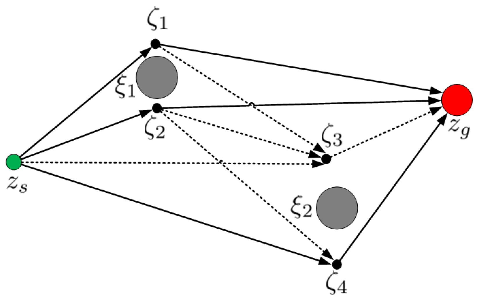
4.1. Homology Classes

The trajectory, characterized by a succession of the robot’s positions in the plane without regard to orientation, is denoted as $\tau =\{z_k\in {\mathbb{R}}^2\mid k=1,2,\dots ,N\}$. The transformation from this initial trajectory to the optimization parameter x is articulated by the function $x=h\left(\tau \right)$. Two paths ${ø}_{\mathit{1}}$ and ${ø}_{\mathit{2}}$ are said to be in the same homotopy class $\mathit{iff}$ one can be smoothly deformed into the other without intersecting obstacles. Otherwise, they are categorized into different homotopy classes [35]. Calculating homotopy classes in closed form is generally challenging. Reference [36] advocates the employment of homology classes in lieu of traditional methods, citing their computational tractability. These classes encompass a set of trajectories that are homologous to each other as delineated in [37]. The determination of homology classes through an analytical lens, grounded in complex analysis, is elaborated upon in [35,36]. Succinctly, the homology invariant, termed the H-signature, creates an equivalence relation by allocating a distinct complex number to each trajectory within an identical homology class, thereby differentiating them.

With the robot’s current location denoted by $z_s$ and the target position by $z_g$ (expressed in complex number notation $\mathbb{C}$), along with the compilation of obstacle regions $\mathcal{O}=\{{\mathcal{O}}_l\mid l=1,2,\dots ,R\}$, an exploration graph $\mathcal{G}=\mathcal{V}$, $\epsilon$ is meticulously constructed. This graph serves to identify an initial set of viable paths. The vertices within this graph are specified as follows:

$$\mathcal{V}=z_s,{\zeta }_i,z_g\in \mathbb{C}\mid \forall {\zeta }_i\notin \mathcal{O},i=1,2,\cdots ,I$$

(12)

In this context, ${\zeta }_i\in \mathbb{C}$ represents potential waypoints that can be incorporated into the trajectory. The initial phase of exploration is dedicated to generating waypoints that lie between the starting point $z_s$ and the destination $z_g$. To simplify the model, obstacles are presumed to have a circular form with a predefined radius. Opposite each obstacle, and perpendicular to the line segment connecting $z_s$ and $z_g$, a pair of prospective waypoints is strategically positioned to the left and right. This initial setup is adequate for generating a subset of unique and viable paths. Figure 2 provides a schematic representation of the obstacle configuration and the corresponding waypoint candidates within a sample environment, where ${\xi }_l\in {\mathcal{O}}_l$ signifies the pivotal point representing each obstacle, and the circle centered at ${\xi }_l$ delineates the obstacle region ${\mathcal{O}}_l$.

Figure 2. Example of an exploration graph. The green circle represents the current position. The red circle represents the goal. The gray circle represents obstacles. The black circle represents the waypoint.

The construction of the edge set $\epsilon$ is derived from the initial waypoint seeds. An edge is established between two vertices $v_1\in \mathcal{V}$ and $v_2\in \mathcal{V}$ on the condition that the following criteria are satisfied:

(1) The edge direction aligns with the forward progress towards the goal, ensuring that the real part of the complex number product $\overline{(v_2-v_1)}(z_g-z_s)$ divided by the product of the magnitudes $|v_2-v_1|$ and $|z_g-z_s|$ exceeds a threshold angle $\theta$, where $\theta$ is a value within the interval $[0,1]$.

(2) The line segment $\mathcal{L}$, defined as $\{v_1+t(v_2-v_1)\mid t\in [0,1]\}$, must not intersect with any obstacle regions ${\mathcal{O}}_l$, implying that the intersection of $\mathcal{L}$ and $\mathcal{O}$ is an empty set $\mathcal{L}\cap \mathcal{O}=\varnothing$.

The initial criterion eliminates trajectories where the Euclidean distance to the target point does not exhibit a strictly decreasing pattern. Online trajectory planners frequently devise intermediate objectives, which are assumed to be systematically organized by a global planning mechanism. Given the orderly arrangement of these subsidiary goals, the limitation to acyclic graph structures is deemed appropriate. This stipulation substantially diminishes both the volume of potential trajectories and the computational demands associated with graph traversal. The angular threshold $\theta$, dictating the forward direction’s field of view, can be adjusted upwards to further constrict the visual scope. The edges, as illustrated in the preceding example, are depicted in Figure 2.

4.2. Homology Class Path Generation

Utilizing the constructed graph $\mathcal{G}$, we employ an augmented depth-first search, supplemented by a record of visited nodes, to extract direct paths between the starting point $z_s$ and the target point $z_g$. For each identified path, the H-signature is calculated; if it is not already present in our repository, it is added to the collection of known signatures [38]. Paths that exhibit identical H-signatures are eliminated to ensure uniqueness. To enhance computational efficiency, the processes of retrieving all straightforward routes and sieving for homologous paths are consolidated into a unified search algorithm. Algorithm 1 delineates our enhanced recursive depth-first search approach. The trajectory set is referenced by T, while B encompasses the nodes visited thus far, ultimately forming the complete trajectory from $z_s$ to $z_g$ upon reaching the goal. This trajectory is then cross referenced with the homology class set H to detect any duplicates. Should it represent a novel homology class, the optimization problem’s corresponding trajectory is initialized based on the path B. The initial trajectory, defined by the sequence $\{z_s,{\zeta }_i,z_g\}$, is subjected to further refinement through subsampling, with the orientation of each pose being aligned with the direction of the subsequent positions. We opt to store the entire optimization parameter x rather than just the 2D position $\tau$ of the trajectories, facilitating the subsequent rapid reinitialization of the optimization process. To curtail the processing time, the algorithm is designed to recognize a predefined maximum of distinct topological configurations as indicated in line 2.

Algorithm 1: Homology class path generation.

Input: $\mathcal{G}$, B, $z_g$; T; H Output: Updated set of trajectories and H-signatures

    Waypoint sampling follows the Probabilistic Roadmap (PRM) planner [39]. The PRM planner leverages a learned graph of the free space to search for an obstacle-free path from the robot’s current location to the target [40]. The initial graph is constructed using a generalized inverse kinematics algorithm based on the Levenberg–Marquardt (LM) method [41]. The initial path is then converted into a regularly spaced series of waypoints, or steps, at intervals shorter than the length of the robot.

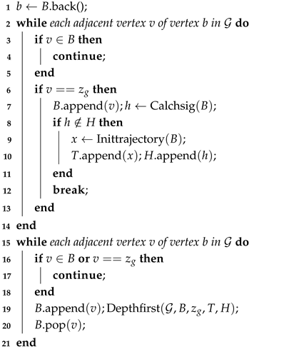
4.3. CE Trajectory Optimization

The CE method is an importance sampling (IS) technique used for Estimating Rare Events (ERE) [42]. The essence of the CE method is to frame the optimization of the function $J\left(z\right)$ with a real-valued cost as a rare event estimation problem. The optimal cost function is denoted by ${\gamma }^{*}$:

$${\gamma }^{*}=\underset{z\in Ƶ}{min}J\left(z\right)$$

(13)

The core of the CE method involves the multi-level sampling of parameter sequences ${\left\{v_j\right\}}_{j\ge 0}$ and ${\left\{{\gamma }_j\right\}}_{j\ge 1}$. This sequence converges to the optimal $v^{*}$, which can then be used to estimate the integral $\widehat{\ell }$. The following describes a trajectory optimization algorithm based on the CE method, with the parameter space defined as follows:

$$\mathcal{V}={\left({\mathbb{R}}^{n_z}\times {\mathbb{R}}^{\left(n_z^2+n_z\right)/2}\right)}^K\times {\mathbb{R}}^K$$

(14)

where the element $v=\left({\mu }_1,{\Sigma }_1,\dots ,{\mu }_K,{\Sigma }_K,w_1,\dots ,w_K\right)$ corresponds to K mixture components, each with mean ${\mu }_k$, covariance matrix ${\Sigma }_k$, and weight $w_k$. The density is defined as

$$p(z;v)=\sum _{k=1}^K{\displaystyle \frac{w_k}{\sqrt{{\left(2\pi \right)}^{n_z}\left|{\Sigma }_k\right|}}}{e}^{-{\displaystyle \frac{1}{2}}{\left(\epsilon -{\mu }_k\right)}^T{\Sigma }_k^{-1}\left(\epsilon -{\mu }_k\right)}$$

(15)

where ${\sum }_{k=1}^K{w}_k=1$. The CE trajectory optimization algorithm is illustrated in Algorithm 2.

Algorithm 2: CE trajectory optimization.

Input: $z^{*},\Sigma$ Output: $\widehat{v}$

To achieve comprehensive coverage of $\mathcal{X}$, an initial sample set is generated. This initial sampling is obtained through the Homology Class Planner discussed in the previous subsection, and the initial trajectory $z^{*}$ is computed. A normal distribution $\Sigma$ with covariance centered at $z^{*}$ is selected to cover the relevant reachable space and produce the initial sample set. When $K⩾2$, the Expectation–Maximization (EM) algorithm is employed to achieve optimal parameter updates. For $K=1$, the components of ${\widehat{v}}_j$ are updated simply as follows:

$$\mu ={\displaystyle \frac{1}{\left|{\mathcal{E}}_j\right|}}\sum _{Z_k\in {\mathcal{E}}_j}{Z}_k,\Sigma ={\displaystyle \frac{1}{\left|{\mathcal{E}}_j\right|}}\sum _{Z_k\in {\mathcal{E}}_j}\left(Z_k-\mu \right){\left(Z_k-\mu \right)}^T$$

(16)

As the algorithm iterates, the determinants of the covariances converge towards a delta distribution.

In Algorithm 2, the sampling process utilizes the accept–reject sampling method, which generates samples through ${Ƶ}_{con}$. The algorithm terminates when the distributional changes between iterations are less than a specified small constant $ϵ$. The algorithm also terminates if the GMM covariances nearly shrink to zero.

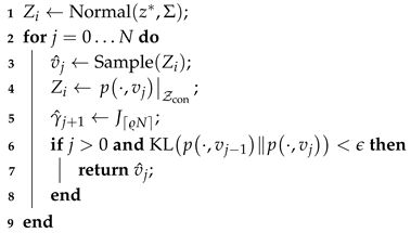
4.4. VSRRT* Path Optimization

The RRT algorithm is initialized with a tree containing the initial state as a single vertex and no edges [43]. At each iteration, a state $x_{rand}$ is sampled from a uniform distribution, which attempts to connect to the nearest vertex $x_{nearest}$ in the tree. If this connection is successful, $x_{rand}$ is adjusted to $x_{new}$ using a steering function. Subsequently, $x_{new}$ is added to the vertex set, and the edge $(x_{nearest},x_{new})$ is included in the edge set. The algorithm continues until the tree contains a state within the goal region or the number of iterations reaches a predefined threshold.

In contrast to the RRT, the RRT* algorithm incorporates two additional procedures: ChooseParent within the Extend $(\mathcal{T},x_{new})$ function and the Rewire process [44]. The asymptotic optimality of RRT* is guaranteed as the number of iterations approaches infinity.

The VSRRT* path optimization algorithm is illustrated in Algorithm 3. The primary difference lies in the tree extension process. When a point $x_{nearest}$ is generated, instead of moving from this point to $x_{rand}$ with limited step size, we directly connect the two points, creating a line l. If l passes the collision-checking process, it is added to the tree. If l collides, the last point along the line will be $x_{new}$, and this point, along with the line between $x_{new}$ and $x_{nearest}$, will be added to the tree.

Algorithm 3: VSRRT* Planner.

Input: $x_{init}$, $\mathcal{G}\left(x_{goal}\right)$, T Output: $\mathcal{T}$

The advantage of our method is that there is no need to adjust the parameter $\sigma$ across different environments. Additionally, by attempting to extend the tree with the largest step size, the planner can cover the configuration space with relatively fewer sampling points, thereby saving time on collision checks for sampling points and finding the nearest point in the existing tree.

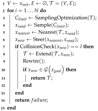
4.5. GMM Sampling Optimization

The sampling space optimization mainly involves controlling the sampling space and using probabilistic sampling with a Gaussian Mixture Model (GMM). A VSRRT* trajectory is represented as a sample from a vector-valued Gaussian Process (GP), $x\left(t\right)\sim \mathcal{GP}(\mu \left(t\right),K(t,t^{\prime }))$, with mean $\mu \left(t\right)$ and covariance $K(t,t^{\prime })$, generated by a linear time-varying stochastic differential equation:

$$\dot{x}\left(t\right)=A\left(t\right)x\left(t\right)+u\left(t\right)+F\left(t\right)w\left(t\right)$$

(17)

where A and F are system matrices, u is a known control input, and $w\left(t\right)\sim \mathcal{GP}(0,Q_c\delta (t-t^{\prime }))$ is a white noise process with power spectral density matrix $Q_c$. Using this stochastic differential equation, the mean and covariance of the GP can be specified as follows:

$$\mu \left(t\right)=\Phi (t,t_0){\mu }_0+{\int }_{t_0}^t\Phi (t,s)u\left(s\right)ds$$

(18)

$$\begin{array}{cc}\hfill K(t,t^{\prime })& =\Phi (t,t_0)K_0\Phi {(t^{\prime },t_0)}^{\top }+{\int }_{t_0}^{min(t,t^{\prime })}\Phi (t,s)F\left(s\right)Q_{c}F{\left(s\right)}^{\top }\Phi (t^{\prime },s)ds\hfill \end{array}$$

(19)

where $\Phi$ is the state transition matrix, and ${\mu }_0$ and $K_0$ are the initial mean and covariance. This trajectory is Gauss–Markov, and a set of VSRRT* trajectories can be represented as samples from the GMM.

The GMM can be described by $\mu$, $\Sigma$ and p, represented as

$$p\left(x\right)=\sum _{i=1}^n{p}_i\mathcal{N}\left({\mu }_i,{\Sigma }_i\right),\sum _{i=1}^n{p}_i=1$$

(20)

where $\mathcal{N}$ denotes a two-dimensional Gaussian distribution, and $p_i$ is the weight of the i-th component. $x=(x_1,x_2)$ is a two-dimensional vector (with $x_1$ and $x_2$ corresponding to the horizontal and vertical directions in the sampling coordinate system), ${\mu }_i$ is a two-dimensional mean vector, and ${\Sigma }_i$ is a $2\times 2$ covariance matrix.

For the covariance matrix $\Sigma =\left[\begin{array}{cccc}{\delta }_1& {\delta }_2;& {\delta }_3& {\delta }_4\end{array}\right]$, if ${\delta }_2$ and ${\delta }_3$ are non-zero, the Gaussian distribution will not be symmetric relative to the axes. For simplicity, we assume ${\delta }_2={\delta }_3=0$, so $\Sigma$ becomes

$$\Sigma =\left[\begin{array}{cc}{\delta }_1& 0\\ 0& {\delta }_2\end{array}\right]$$

(21)

where ${\delta }_1$ and ${\delta }_2$ denote the standard deviations of the Gaussian distribution in the horizontal and vertical directions.

The sampling optimization algorithm is outlined in Algorithm 4. The TrajectoryPoints$\left(T\right)$ function is a preprocessing step in the sampling optimization algorithm, where the mean vector $\mu$ is calculated based on the points of the trajectory $\left(T\right)$. The Update$\left(\mu \right)$ function updates $\left(\mu \right)$, while the Expand$(\Sigma )$ function updates $(\Sigma )$. The sampling space is restricted by probabilistic sampling with the GMM.

Algorithm 4: $\mathrm{SamplingOptimization}\left(T\right)$.

Input: $T,\Sigma$   Output: $C_{limit}$ 1 $\mu \leftarrow \mathrm{TrajectoryPoints}\left(T\right)$; 2 $\Sigma \leftarrow \mathrm{Expand}(\Sigma )$; 3 $\mu \leftarrow \mathrm{Update}\left(\mu \right)$; 4 $C_{limit}\leftarrow \mathrm{GMM}(\Sigma ,\mu )$; 5 return $C_{limit}$;

4.6. TACE-Based Path-Planning Algorithm

The TACE algorithm is a motion planning method based on the CE approach, designed to find optimal paths in nonlinear robotic systems. This method combines sampling-based motion planning with stochastic optimization techniques, leveraging the CE approach to estimate the probability of rare events and utilizing the enhanced VSRRT* optimal motion planning method to navigate complex environments. The core idea behind CE motion planning is to generate new paths using the CE method and update the probability distribution based on the performance of these paths to approximate the optimal solution. In each iteration, CE motion planning generates new paths and uses them to update the probability distribution, continuing this process until a specified convergence criterion is met. By using CE motion planning, optimal paths in complex environments can be found, and the method can balance the computation time and result quality by adjusting the convergence criterion to handle multiple constraints.

The TACE algorithm is outlined in Algorithm 5. This algorithm is based on the CE update, using the density $p_{Ƶ}$ defined in the space of trajectory parameters $z\in Ƶ$. It samples trajectories based on this density, extracts states from these trajectories, and uses them as RRT nodes, which can be interpreted as guiding another density in the state space. The main idea of the TACE algorithm is not only to make full use of individual states in the state space but also to exploit the correlations between states along the entire trajectory.

Algorithm 5: TACE-based path-planning algorithm.

Input: ${\eta }_g,N_{min}$ Output: X

5. Experiments

We use three simulated experiments to test the proposed method. The first experiment evaluates TACE, CE, and LQR-CBF-RRT* in dynamic environments. The second experiment validates the obstacle avoidance performance of the TACE algorithm in environments with irregularly moving obstacles. The third experiment alters the environmental conditions by significantly increasing the number of obstacles to validate the performance of the TACE algorithm in complex environments. In simulation environments, we use the simulation of MATLAB R2021a as the simulation engine. The simulation environments are performed on a 64-b Windows 10 operating system with an Industrial Computer with Intel Core i7-10875 CPU and 32 GB of RAM. We apply the same values for the standard parameters of each algorithm. The step size is set to 30 mm, and the maximum number of iterations is 500.

5.1. Comparison Experiment of Path-Planning Algorithms

Simulations are implemented in dynamic obstacles to verify the robustness and effectiveness of the proposed approach. The simulation map is a 20 m × 20 m. The map in simulation includes a dynamic obstacle and a static obstacle to test the planner’s ability to find the optimal path. The dynamic obstacle is the concave pentagon on the left, which moves toward the upper left corner at a ${45}^{\circ }$ angle. The static obstacle is the convex pentagon on the right.

In simulation environments, we demonstrate the performance and generality of the TACE through several numerical simulations, and compare with CE and LQR-CBF-RRT*. Each simulation is repeated in 20 runs, and the average values of path length, number of large-scale turns, and computation time required to converge to the optimal path are reported.

In the scenario mentioned in the previous section, experiments are conducted on algorithms TACE, CE and LQR-CBF-RRT*, and the experimental results are shown in Figure 3, Figure 4 and Figure 5. The following provides a detailed analysis of the algorithm path lengths and running time parameters based on the experimental results above.

Figure 3. Simulation results of the TACE algorithm. Figures (a–j) are dynamic path trajectory diagrams generated by the TACE algorithm, each representing the result after the obstacle has moved 10 times. The solid black lines represent the obstacle. The red lines represent the branch on the extended tree. The green lines represent the final path. The blue lines represent the sampling area after iteration-based GMM.

Figure 4. Simulation results of the CE algorithm. Figures (a–j) are dynamic path trajectory diagrams generated by the CE algorithm, each representing the result after the obstacle has moved 10 times. The solid black lines represent the obstacle. The dashed black lines are the final trajectory after 5 iterations.

Figure 5. Simulation results of the LQR-CBF-RRT* algorithm. Figures (a–j) are dynamic path trajectory diagrams generated by the LQR-CBF-RRT* algorithm, each representing the result after the obstacle has moved, for a total of 10 times. The solid grey lines represent the obstacle. The green lines represent the branch on the extended tree. The red lines represent the final path.

Figure 6 compares the path lengths between the TACE, CE, and LQR-CBF-RRT* algorithms. Figure 6 shows that the TACE algorithm produces shorter paths in all cases compared to the CE and LQR-CBF-RRT* algorithms over 5 rounds. Figure 7 compares the running times between the TACE, CE, and LQR-CBF-RRT* algorithms. Figure 7 indicates that although the TACE algorithm has a longer running time than the CE algorithm, it is faster than the LQR-CBF-RRT* algorithm, with shorter running times. Compared with the CE algorithm, the TACE algorithm significantly sacrifices the shorter computation time to improve path accuracy. By analyzing Figure 6 and Figure 7, we see that all path planners ensure the effective finding of the path solutions. Among them, our proposed algorithm provides the best path-planning performance.

Figure 6. Comparison of algorithm path lengths. The 10 images represent different scenarios generated by moving the obstacle 10 times. The horizontal axis indicates the number of iterations, with the TACE and LQR-CBF-RRT* algorithms iterating 100 times per round. The vertical axis represents the trajectory length from the starting point to the target point. The solid red line represents the TACE algorithm, the green dotted line represents the CE algorithm, and the blue dashed line represents the LQR-CBF-RRT* algorithm.

Figure 7. Comparison of the algorithm running time. The horizontal axis represents Case 1 to Case 10 generated by moving the obstacle 10 times. The vertical axis represents the total running time of the algorithm at the end of the iterations. The solid red line represents the TACE algorithm, the green dotted line represents the CE algorithm, and the blue dashed line represents the LQR-CBF-RRT* algorithm.

In the experimental results, the TACE algorithm has a shorter running time than the LQR-CBF-RRT* algorithm, showing the effectiveness of the precomputed homology paths based on the Homology Class Planner and the probabilistic sampling method based on the GMM. With an equal number of iterations to TACE, the sampling space calculated by LQR-CBF-RRT* has a large area and fails to minimize the useless space. Due to shorter path lengths, TACE executes the solution at the lowest execution cost. The TACE path is a global optimal path rather than a local optimal path by homology class path generation and VSRRT*-based path optimization. As shown in Figure 5, the paths generated by LQR-CBF-RRT* are usually tortuous, with longer path lengths and more large-scale turns. Although the paths obtained by CE are not as tortuous as those searched by LQR-CBF-RRT*, the path quality is still unsatisfactory, especially regarding the path length.

In contrast, the TACE algorithm finds a smoother path trajectory than other methods, with fewer nodes, local windings, and sharp turns. First, TACE performs better than other methods in a dynamic environment. Second, CE and LQR-CBF-RRT* easily fall into local optima and fail to return optimal solutions. Third, TACE is more effective than LQR-CBF-RRT* in removing useless search space under identical numbers of iterations. In short, our proposed TACE algorithm achieves higher path quality, good robustness, and higher convergence speed than other methods.

5.2. Experiment with Irregularly Moving Obstacle

To validate the obstacle avoidance performance of the TACE algorithm in environments with irregularly moving obstacles, the following experiments are conducted. The experimental map is a 20 m × 20 m. The robot’s path-planning method uses the TACE algorithm. The robot moves from the start point at the bottom-left corner of the map to the goal point at the top-right corner. The initial position of the dynamic obstacles is above the robot. After the robot starts moving, the dynamic obstacles move at the same speed along a random path. Ten frames from the motion process are captured in the experimental results and are shown in Figure 8.

Figure 8. Simulation results of the TACE algorithm in environments with irregularly moving obstacles. (a–j) The 10 frames captured during the motion process. The green dot represents the start point, the red dot represents the goal point, the blue dot represents the robot, and the purple dot represents the dynamic obstacles. The black solid line indicates the robot’s motion trajectory, while the red dashed line represents the motion trajectory of the dynamic obstacles.

Based on the dynamic motion scene shown in Figure 8, we observe that the robot using the TACE algorithm for path planning is able to change its direction to avoid collisions with obstacles. Afterward, it replans an optimal path toward the goal. The simulation experiment demonstrates that the TACE algorithm is both effective and practical, providing valuable insights for enabling robots to navigate around irregularly moving obstacles.

5.3. Experiment with Complex Environments

To verify the obstacle avoidance and planning performance results of the TACE algorithm in complex environments with a large number of obstacles, the following experiments are conducted. The experimental map is a 20 m × 20 m. The robot’s path-planning method uses the TACE algorithm. The robot moves from the start point at the bottom-left corner of the map to the goal point at the top-right corner. The experimental results are shown in Figure 9.

Figure 9. Simulation results of the TACE algorithm in complex environments. (a–d) The path trajectories at iteration numbers 100, 200, 400, and 500, respectively. The black squares represent obstacles. The red lines represent the branch on the extended tree. The green lines represent the final path. The blue lines represent the sampling area after iteration-based GMM.

Figure 9 illustrates the iterative process of the TACE algorithm generating paths with increasing precision. As the number of iterations increases, the accuracy of the paths improves. This experiment also demonstrates that when environmental conditions change, such as an increase in obstacles, the TACE algorithm can still effectively and accurately plan the path.

6. Conclusions and Future Work

In this paper, we have introduced a topology-aware approach to efficient path planning in dynamic environments. The key idea is to leverage topological information to enhance traditional path-planning methods, allowing for more robust and efficient navigation in the presence of dynamic obstacles. Our approach integrates dynamic environment changes into the path-planning process, enabling real-time updates while maintaining path optimality. Experimental results demonstrate that the proposed method outperforms conventional path-planning techniques in terms of computation time and the quality of the generated paths. The topology-aware information significantly improves navigation efficiency in dynamic and unpredictable environments. Future work will focus on refining the algorithm to handle more complex environments with higher levels of uncertainty. Additionally, incorporating advanced prediction models for dynamic obstacles could further improve performance and ensure greater adaptability in real-world scenarios.

References

- Yang, L.; Li, P.; Qian, S.; Quan, H.; Miao, J.; Liu, M.; Hu, Y.; Memetimin, E. Path Planning Technique for Mobile Robots: A Review. Machines 2023, 11, 980. [Google Scholar] [CrossRef]
- Wang, C.; Meng, L.; She, S.; Mitchell, I.M.; Li, T.; Tung, F.; Wan, W.; Meng, M.Q.H.; de Silva, C.W. Autonomous Mobile Robot Navigation in Uneven and Unstructured Indoor Environments. In Proceedings of the 2017 IEEE/RSJ International Conference on Intelligent Robots and Systems (IROS), Vancouver, BC, Canada, 24–28 September 2017; pp. 109–116. [Google Scholar]
- Wang, C.; Ma, H.; Chen, W.; Liu, L.; Meng, M.Q.H. Efficient Autonomous Exploration with Incrementally Built Topological Map in 3-D Environments. IEEE Trans. Instrum. Meas. 2020, 69, 9853–9865. [Google Scholar] [CrossRef]
- Khatib, O. Real-time obstacle avoidance for manipulators and mobile robots. Int. J. Robot. Res. 1986, 5, 90–98. [Google Scholar] [CrossRef]
- Yu, J.; Wu, J.; Xu, J.; Wang, X.; Cui, X.; Wang, B.; Zhao, Z. A Novel Planning and Tracking Approach for Mobile Robotic Arm in Obstacle Environment. Machines 2024, 12, 19. [Google Scholar] [CrossRef]
- Baumgartner, J.; Petrič, T.; Klančar, G. Potential Field Control of a Redundant Nonholonomic Mobile Manipulator with Corridor-Constrained Base Motion. Machines 2023, 11, 293. [Google Scholar] [CrossRef]
- Li, J.; Zhai, X.; Xu, J.; Li, C. Target Search Algorithm for AUV Based on Real-Time Perception Maps in Unknown Environment. Machines 2021, 9, 147. [Google Scholar] [CrossRef]
- Hart, P.E.; Nilsson, N.J.; Raphael, B. A formal basis for the heuristic determination of minimum cost paths. IEEE Trans. Syst. Sci. Cybern. 1968, 4, 100–107. [Google Scholar] [CrossRef]
- Dijkstra, E.W. A note on two problems in connexion with graphs. Numer. Math. 1959, 1, 269–271. [Google Scholar] [CrossRef]
- Wang, C.; Li, T.; Meng, M.Q.H.; De Silva, C. Efficient Mobile Robot Exploration with Gaussian Markov Random Fields in 3D Environments. In Proceedings of the 2018 IEEE International Conference on Robotics and Automation (ICRA), Brisbane, QLD, Australia, 21–25 May 2018; pp. 5015–5021. [Google Scholar]
- Wang, C.; Zhu, D.; Li, T.; Meng, M.Q.H.; De Silva, C.W. Efficient Autonomous Robotic Exploration with Semantic Road Map in Indoor Environments. IEEE Robot. Autom. Lett. 2019, 4, 2989–2996. [Google Scholar] [CrossRef]
- Wang, C.; Chi, W.; Sun, Y.; Meng, M.Q.H. Autonomous Robotic Exploration by Incremental Road Map Construction. IEEE Trans. Autom. Sci. Eng. 2019, 16, 1720–1731. [Google Scholar] [CrossRef]
- Chi, W.; Wang, C.; Wang, J.; Meng, M.Q.H. Risk-DTRRT-Based Optimal Motion Planning Algorithm for Mobile Robots. IEEE Trans. Autom. Sci. Eng. 2019, 16, 1271–1288. [Google Scholar] [CrossRef]
- Dong, Z.; Zhong, B.; He, J.; Gao, Z. Dual-Arm Obstacle Avoidance Motion Planning Based on Improved RRT Algorithm. Machines 2024, 12, 472. [Google Scholar] [CrossRef]
- Cui, Y.; Zhang, Q.; Feng, Z.; Wei, Z.; Shi, C.; Yang, H. Topology-aware resilient routing protocol for FANETs: An adaptive Q-learning approach. IEEE Internet Things J. 2022, 9, 18632–18649. [Google Scholar] [CrossRef]
- Englot, B.; Hover, F.S. Three-dimensional coverage planning for an underwater inspection robot. Int. J. Robot. Res. 2013, 32, 1048–1073. [Google Scholar] [CrossRef]
- Janson, L.; Schmerling, E.; Clark, A.; Pavone, M. Fast marching tree: A fast marching sampling-based method for optimal motion planning in many dimensions. Int. J. Robot. Res. 2015, 34, 883–921. [Google Scholar] [CrossRef]
- Salzman, O.; Halperin, D. Asymptotically near-optimal RRT for fast, high-quality motion planning. IEEE Trans. Robot. 2016, 32, 473–483. [Google Scholar] [CrossRef]
- Chen, L.; Shan, Y.; Tian, W.; Li, B.; Cao, D. A Fast and Efficient Double-Tree RRT*-like Sampling-Based Planner Applying on Mobile Robotic Systems. IEEE/ASME Trans. Mechatron. 2018, 23, 2568–2578. [Google Scholar] [CrossRef]
- Elbanhawi, M.; Simic, M.; Jazar, R. Randomized Bidirectional B-Spline Parameterization Motion Planning. IEEE Trans. Intell. Transp. Syst. 2016, 17, 406–419. [Google Scholar] [CrossRef]
- Suh, J.; Gong, J.; Oh, S. Fast Sampling-Based Cost-Aware Path Planning with Nonmyopic Extensions Using Cross Entropy. IEEE Trans. Robot. 2017, 33, 1313–1326. [Google Scholar] [CrossRef]
- Zhao, H.; Wang, C.; Guo, R.; Rong, X.; Guo, J.; Yang, Q.; Yang, L.; Zhao, Y.; Li, Y. Autonomous live working robot navigation with real-time detection and motion planning system on distribution line. High Volt. 2022, 7, 1204–1216. [Google Scholar] [CrossRef]
- Wang, J.; Chi, W.; Shao, M.; Meng, M.Q.H. Finding a High-Quality Initial Solution for the RRTs Algorithms in 2D Environments. Robotica 2019, 37, 1677–1694. [Google Scholar] [CrossRef]
- Zha, F.; Liu, Y.; Wang, X.; Chen, F.; Li, J.; Guo, W. Robot motion planning method based on incremental high-dimensional mixture probabilistic model. Complexity 2018, 2018, 1–14. [Google Scholar] [CrossRef]
- Huh, J. Learning Probabilistic Generative Models for Fast Sampling-Based Planning. Ph.D. Thesis, University of Pennsylvania, Philadelphia, PA, USA, 2019. [Google Scholar]
- Zhao, X.; Zhao, H.; Wan, S.; Ding, H. A Gaussian Mixture Models based Multi-RRTs method for high-dimensional path planning. In Proceedings of the 2018 IEEE International Conference on Robotics and Biomimetics (ROBIO), Kuala Lumpur, Malaysia, 12–15 December 2018; pp. 1659–1664. [Google Scholar]
- Yu, F.; Chen, Y. Cyl-IRRT*: Homotopy optimal 3D path planning for AUVs by biasing the sampling into a cylindrical informed subset. IEEE Trans. Ind. Electron. 2022, 70, 3985–3994. [Google Scholar] [CrossRef]
- Tao, X.; Lang, N.; Li, H.; Xu, D. Path planning in uncertain environment with moving obstacles using warm start cross entropy. IEEE/ASME Trans. Mechatron. 2021, 27, 800–810. [Google Scholar] [CrossRef]
- Ahmad, A.; Belta, C.; Tron, R. Adaptive sampling-based motion planning with control barrier functions. In Proceedings of the 2022 IEEE Conference on Decision and Control (CDC), Cancun, Mexico, 6–9 December 2022; pp. 4513–4518. [Google Scholar]
- Yang, G.; Cai, M.; Ahmad, A.; Prorok, A.; Tron, R.; Belta, C. LQR-CBF-RRT*: Safe and optimal motion planning. arXiv 2023, arXiv:2304.00790. [Google Scholar]
- Chi, W.; Ding, Z.; Wang, J.; Chen, G.; Sun, L. A generalized Voronoi diagram-based efficient heuristic path planning method for RRTs in mobile robots. IEEE Trans. Ind. Electron. 2021, 69, 4926–4937. [Google Scholar] [CrossRef]
- Wang, J.; Meng, M.Q.H. Optimal path planning using generalized voronoi graph and multiple potential functions. IEEE Trans. Ind. Electron. 2020, 67, 10621–10630. [Google Scholar] [CrossRef]
- Yuan, Y.; Liu, J.; Chi, W.; Chen, G.; Sun, L. A Gaussian mixture model based fast motion planning method through online environmental feature learning. IEEE Trans. Ind. Electron. 2022, 70, 3955–3965. [Google Scholar] [CrossRef]
- Liu, J.; Fu, M.; Liu, A.; Zhang, W.; Chen, B. A Homotopy Invariant Based on Convex Dissection Topology and a Distance Optimal Path Planning Algorithm. IEEE Robot. Autom. Lett. 2023, 8, 7695–7702. [Google Scholar] [CrossRef]
- Bhattacharya, S.; Kumar, V.; Likhachev, M. Search-Based Path Planning with Homotopy Class Constraints. In Proceedings of the AAAI Conference on Artificial Intelligence (AAAI), Atlanta, GA, USA, 11–15 July 2010; AAAI Press: Palo Alto, CA, USA, 2010; pp. 1230–1237. [Google Scholar]
- Bhattacharya, S. Topological and Geometric Techniques in Graph Search-Based Robot Planning. Ph.D. Thesis, University of Pennsylvania, Philadelphia, PA, USA, 2012. [Google Scholar]
- Rösmann, C.; Hoffmann, F.; Bertram, T. Planning of multiple robot trajectories in distinctive topologies. In Proceedings of the 2015 European Conference on Mobile Robots (ECMR), Lincoln, UK, 2–4 September 2015; pp. 1–6. [Google Scholar]
- Rösmann, C.; Hoffmann, F.; Bertram, T. Integrated online trajectory planning and optimization in distinctive topologies. Robot. Auton. Syst. 2017, 88, 142–153. [Google Scholar]
- Sarah, K.; Gerard, C.; Michael, C. Task-Aware Waypoint Sampling for Planning Robots. In Proceedings of the International Conferenceon Automated Planning and Scheduling (ICAPS), Guangzhou, China, 7–12 June 2021; pp. 643–651. [Google Scholar]
- Kavraki, L.E.; Svestka, P.; Latombe, J.C.; Overmars, M.H. Probabilistic roadmaps for path planning in high-dimensional configuration spaces. IEEE Trans. Robot. Autom. 1996, 12, 566–580. [Google Scholar] [CrossRef]
- Rösmann, C.; Hoffmann, F.; Bertram, T. Kinodynamic trajectory optimization and control for car-like robots. In Proceedings of the 2017 IEEE/RSJ International Conference on Intelligent Robots and Systems (IROS), Vancouver, BC, Canada, 24–28 September 2017; pp. 5681–5686. [Google Scholar]
- Kobilarov, M. Cross-entropy motion planning. Int. J. Robot. Res. 2012, 31, 855–871. [Google Scholar] [CrossRef]
- LaValle, S.M.; Kuffner, J.J., Jr. Randomized Kinodynamic Planning. Int. J. Robot. Res. 2001, 20, 378–400. [Google Scholar] [CrossRef]
- Karaman, S.; Frazzoli, E. Sampling-Based Algorithms for Optimal Motion Planning. Int. J. Robot. Res. 2011, 30, 846–894. [Google Scholar] [CrossRef]
Disclaimer/Publisher’s Note: The statements, opinions and data contained in all publications are solely those of the individual author(s) and contributor(s) and not of MDPI and/or the editor(s). MDPI and/or the editor(s) disclaim responsibility for any injury to people or property resulting from any ideas, methods, instructions or products referred to in the content. |
© 2024 by the authors. Licensee MDPI, Basel, Switzerland. This article is an open access article distributed under the terms and conditions of the Creative Commons Attribution (CC BY) license (https://creativecommons.org/licenses/by/4.0/).